FindingEmo: An Image Dataset for Emotion Recognition in the Wild

Abstract

We introduce FindingEmo, a new image dataset containing annotations for 25k images, specifically tailored to Emotion Recognition. Contrary to existing datasets, it focuses on complex scenes depicting multiple people in various naturalistic, social settings, with images being annotated as a whole, thereby going beyond the traditional focus on faces or single individuals. Annotated dimensions include Valence, Arousal and Emotion label, with annotations gathered using Prolific. Together with the annotations, we release the list of URLs pointing to the original images, as well as all associated source code.

1 Introduction

Computer vision has known an explosive growth over the past decade, most notably due to the resurgence of Artificial Neural Networks. For many vision-related tasks, computer models have been developed that match or exceed human performance, e.g., image classification (He et al., 2015) and mammographic screening (McKinney et al., 2020). Many of these tasks, however, are relatively simplistic in nature: detecting the absence or presence of an object, or naming an item in the picture. When it comes to more complex tasks, Artificial Intelligence (AI) still has a long way to go. Affective Computing (Picard, 1997), a field that combines disciplines such as computer science and cognitive psychology to study human affect and attempt to make computers understand emotions, is an example of such a complex problem. This paper is concerned in particular with the subtask of Emotion Recognition, which revolves around building AI models that manages to recognize the emotional state of individuals from numerical data, in our case pictures. This particular problem has been gaining traction over the past years, as it has many applications, ranging from psychology (Cowie et al., 2001), to human-computer interaction (Emanuel & Eldar, 2023), to robotics (Spezialetti et al., 2020).

Further complicating the matter is the fact that in the field of psychology, the concept of what an emotion is exactly is heavily debated (Barrett, 1998; Barrett et al., 2009; Harmon-Jones et al., 2017), resulting in several ways of describing emotions, either by means of continuous dimensions (Russell, 1980; Mehrabian, 1996), or by means of labels, with different competing label classification schemes existing (Ekman, 1970; Plutchik, 1980; Scherer, 2005).

Figure 1: Logo for the FindingEmo dataset.

The application of computer vision techniques toward Emotion Recognition has historically largely focused on detecting emotions from human facial expressions, with the problem still being actively investigated (Tian et al., 2001; Zhao & Pietikainen, 2007; Zhang et al., 2012, 2018; Zhu et al., 2020; Zhang et al., 2021; Huang et al., 2023). However, the importance of context in emotion recognition is increasingly being acknowledged in psychology (Aviezer et al., 2012; Kumfor et al., 2018). This led to the release of the computer vision dataset EMOTIC (Kosti et al., 2019), presenting photos of people in natural settings, rather than face-focused close-ups, and leading the way to more complex ANN systems that attempt to combine multiple information streams extracted from these images (Mittal et al., 2020; Thuseethan et al., 2022; Yang et al., 2022).

Nevertheless, even these more recent efforts focus on the emotional state of one particular individual within the picture. In this paper, we present the FindingEmo dataset, which is the first to target higher-order social cognition. Each image in the dataset depicts multiple people in a specific social setting, and has been annotated for the overall emotional content of the entire scene, instead of focusing on a single individual. We hope this data can be used by AI practitioners and psychologists alike to further the understanding of Emotion Recognition, and more broadly, Social Cognition. This is a complex process, consisting of many layers. Consider, e.g., the photograph depicted in Figure 2. Looking only at the bride’s face, one could easily assume she is very sad, or even distressed. Taking also her wedding gown into account, a positive setting is suddenly suggested; perhaps her tears are tears of joy? Only when looking at the full picture does it become clear that the bride is overcome with emotion in a positive way, as conveyed by the setting, the groom reading a prepared text and the clearly supportive bystanders. Thus, full understanding of the bride’s emotional state requires the full scene, including the groom and the solemnly smiling bystanders. This example illustrates how Social Cognition involves detection of relevant elements, extracting relations among these and attributing meaning to construct a coherent whole.

The source code for the scraper and annotation interface used to create the dataset are available from our repo at https://gitlab.com/EAVISE/lme/findingemo, together with the URLs of the annotated images, and their corresponding annotations. The logo for the dataset is depicted in Figure 1. For copyright reasons, we do not share the images themselves. Although we only present one URL per image for now, we are currently gathering backup image URLs wherever possible to minimize broken URLs.

The data collection process was approved by the KU Leuven Ethics Committee.

The remainder of the paper is structured as follows. In Section 2 the data collection process and dataset are described in detail. Next, baseline results for emotion, valence and arousal classification based on popular ImageNet ANN architectures are presented in Section 3. We build upon this by investigating the effect of merging the features and predictions of several models in Section 4. Finally, we conclude in Section 5.

2 Dataset

2.1 Dataset Description

The dataset is composed of annotations for 25,869 unique images depicting various people in various, naturalistic, social settings. Each image has been annotated by one annotator, with 655 annotators—a short description of whom can be found in §A.4—contributing annotations. A separate set of 1525 images, each annotated by multiple annotators, is kept private as a test set for potential future challenges. We do however report annotation statistics on this set in §A.5.

Figure 2: An image from the FindingEmo dataset. Photo courtesy The Kitcherens (https://thekitcheners.co.uk/).

In what follows, we list all annotated dimensions.

Valence and Arousal

We used Russell’s continuous Valence and Arousal dimensions (Russell, 1980), although we allowed users to score Valence on an integer scale $[-3,-2,\dots,3]$, and Arousal on a scale $[0,1,\dots,6]$. Note that Arousal was named “Intensity” in our annotation interface, as we felt “Arousal” might be confusing to some users due to a potential sexually charged interpretation.

Emotion

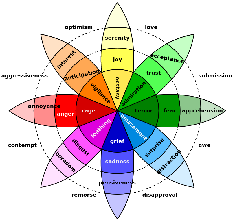
Users had to pick an emotion from Plutchik’s discrete Wheel of Emotions (PWoE) (Plutchik, 1980). We opted for this particular emotion classification scheme as it strikes a balance between the more limited and sometimes contested Ekman’s 6 (Ekman, 1970), and the more expansive, and hence potentially more confusing for annotators, Geneva Emotion Wheel (Scherer, 2005). PWoE defines 24 primary emotions, grouped into 8 groups of 3, where emotions within a group differ in intensity. It is depicted as a flower with the 24 emotions organized in 8 leaves and 3 concentric rings. Each leaf represents a group of 3, with opposite leaves representing opposite emotions. The rings represent the intensity levels, from most intense at the center to least intense at the outside. A depiction can be seen in Figure 3. An additional advantage of PWoE is that one can easily opt to use all 24 emotions, or instead limit oneself to the 8 groups, allowing some granularity control. We refer to these choices as “Emo24” and “Emo8” respectively, and refer to the groups as “emotion leaves” of PWoE.

Figure 3: Plutchik’s Wheel of Emotions.

Age group

Users had to tick one or more boxes from “Children”, “Youth”, “Young Adults”, “Adults” and “Seniors”, indicating the age groups present in the image.

Deciding factor(s) for emotion

Users had to tick one or more boxes from “Neutral”, “Body language”, “Conflict context vs. person”, “Facial expression” and “Staging”, indicating what prompted them to choose for a particular emotion.

Ambiguity

Lastly, users could indicate by means of an integer scale $[0,1,\dots,6]$ how ambiguous the emotional content exhibited by the entire photograph was, or alternatively, how much difficulty they had in annotating the picture.

2.2 Positioning Versus Existing Datasets

Although research in automated Emotion Recognition has been gaining in popularity over the years, progress is still hampered by a lack of data. Earlier work tended to focus solely on recognizing emotions from faces. In their recent review paper, (Khare et al., 2024) list no less than 21 publicly available datasets of facial images for this purpose, typically annotated with Ekman’s 6, potentially extended with a “neutral” category, or custom defined emotion categories. Some of the more popular such datasets, like JAFFE (Lyons et al., 1998) and CK+ (Lucey et al., 2010), make use of a limited number of actors (10 for JAFFE, 123 for CK+) that were instructed to act out a certain emotion, resulting in caricatural emotional expressions.

Publicly available datasets going beyond the face are few in number. First, there is EMOTIC (Kosti et al., 2019), a 23,571 image dataset depicting people in the wild, and with natural expressiveness. An explicit goal of EMOTIC is to take context into account when assessing a person’s emotional state. One or more individual subjects are delineated by a bounding box in each picture for a total of 34,320 subjects, each annotated for Valence, Arousal, Dominance and one of 26 custom defined emotion categories.

CAER-S is a dataset of 70,000 stills taken from 79 TV shows. The stills were extracted from 13,201 video clips that were annotated for Ekman’s 6 + neutral. Each still contains at least one visible face. The aim of the dataset is to allow augmenting facial emotion recognition with contextual features.

Similar to EMOTIC, there is HECO, a dataset of 9,385 images taken from previously released Human-Object Interaction datasets, films and the internet. Like EMOTIC, 19,781 individual subjects were annotated in the pictures for Valence, Arousal, Dominance, 8 discrete emotion categories comprised of Ekman’s 6 + Excitement and Peace, and two novel dimensions, Self-assurance and Catharsis.

Table 1 groups these dataset descriptions, together with ours, for easy comparison.

Table 1: Comparison of datasets for emotion recognition. “Source” refers to the source of the images, “Target” refers to the annotation target, “V/A/D” indicates which of the Valence, Arousal and Dominance dimensions were annotated, “Emotions” refers to what scheme was used to annotate emotions, “Reference” refers to the paper that introduced the dataset.

Name	Nb. images	Source	Target	V/A/D	Emotions	Reference
EMOTIC	23,571	COCO + Ade20k + internet	Single person	V/A/D	26 custom emotion categories	(Kosti et al., 2019)
CAER-S	70,000	TV Shows	Single person (face visible)	–	Ekman’s 6 + neutral	(Lee et al., 2019)
HECO	9,385	HICO-DET + V-COCO + film + internet	Single person	V/A/D	Ekman’s 6 + Excitement and Peace	(Yang et al., 2022)
FindingEmo	25,869	Internet	Whole image	V/A	Plutchik’s Wheel of Emotions	This paper

2.3 Dataset Creation Process

The creation of the dataset was split into two phases. The first phase focused on gathering a large set of images, prioritizing quantity over quality. The second phase consisted in collecting the annotations proper.

2.3.1 Phase 1: Gathering Images

Phase 1 consisted in building a customized, Python-based DuckDuckGo image scraper, programmed to generate random image search queries as follows. Three sets of keywords were defined: one containing a diverse set of emotions; one containing social settings and environments (e.g., ‘birthday’, ‘workplace’, etc.); and one referring to humans (e.g., ‘people’, ‘adults’, ‘youngsters’, etc.). By taking all possible combinations of the elements in these sets, the system generated a multitude of queries, such as, e.g., “happy youngsters birthday”. The first $N$ results were then retrieved and filtered to exclude a number of manually blacklisted domains (e.g., stock photography providers) and by image size. Query results that passed the filtering steps were downloaded.

We started with $N=500$ and image width $800$px $<w<1600$px, and later extended this to $N=1000$ and $800$px $<w<3200$. Obviously, not all downloaded images satisfied our criterion of depicting multiple people in a natural setting. Hence, as a further filtering step, one of the authors annotated 3097 images as either “keep” (useful) or “reject” (no use). These images were used to train a CNN to perform the same task, achieving an accuracy of 77.6%. This model was used to further filter downloaded images: if the CNN labeled the downloaded image as “reject”, the image was discarded.

In total 1,041,105 images were collected.

2.3.2 Phase 2: Gathering Annotations

The annotations were gathered using a custom web interface written in Python, HTML and JavaScript. Annotators were recruited through the Prolific platform. For this, a job would be created, which we refer to as a “run”, to which users could subscribe. After doing so, they received a URL that allowed them to log on to our system and, after agreeing to an Informed Consent clause, perform the annotations. First, users were presented with detailed instructions, a copy of which are provided in §A.1, after which the data collection proper began. To be able to monitor the process closely, and to cope with hardware limitations of our server, we opted to only perform runs with a limited number of participants, most often 15. For each run, the Prolific user selection criteria were the same: fluent English speaker, neurotypical, and a 50/50 split male/female.

In total, annotations were collected over 51 runs. Candidates were informed of an expected task duration of 1h, including reading the instructions, and offered a $\pounds$10 reward. Analysis of the durations (see §A.3) show our time estimation to be fair. We spent a total of $\pounds$10k, which includes annotators whose contributions were filtered out, and most importantly, Prolific fees and taxes.

A screenshot of the interface is included in §A.2. The interface presents users with images on the left side, and dimensions to annotate on the right side. At the top left, users are presented with two buttons: one to skip an image if they so wish, and one to save the current annotation and move on to the next image.

Upon being presented an image, the first choice users needed to make was, just like the filtering CNN, whether to “keep” or “reject” the image, according to the provided instructions. Essentially, users were asked to reject images that contained no people, were watermarked, were of bad quality, etc. If users opted to “reject” an image, no further annotation was needed. This step was needed to further filter images that passed through the CNN. If the choice was “reject”, no further action (besides saving) was required. Optionally, users could choose to select one of several tags indicating why they opted to reject the image from “Bad quality photo”, “Copyright”, “Watermark”, “No interaction”, “No people”, “Text” and “Not applicable”. Each user was asked to annotate 50 “keep” images; “rejects” did not count towards the total goal. Despite this, some users still performed full annotations on images they rejected. If users opted to “keep” the image, they were expected to annotate all other dimensions as well.

Although the frontend (i.e., user interface) remained essentially unchanged, the backend underwent some changes as annotations were collected, and some lessons were learned, which we list here.

Initial iteration

Initially, an image was randomly selected from the corpus, and processed by an updated “keep/reject” CNN (see §2.3.1) with an accuracy of 83.6%. If the “keep” probability $p_{k}$ was $<0.75$, a new random image would be selected and tested, until one was found with $p_{k}\geq 0.75$. If this image had already been annotated, the process would start over, until a valid image was found, which would then be shown to the annotator.

Second iteration

At first, the annotating of all dimensions was not enforced; users could select the “keep” checkbox, save the annotation without annotating anything else, and move on to the next image. Most did their job diligently, but nevertheless we opted to update the interface to require all dimensions be annotated in case of a “keep”, before the “Save” option became available. This frequently prompted messages from users complaining the “Save” option was not available to them. A further update explained this to users who prematurely clicked on the “Save” button.

Third iteration

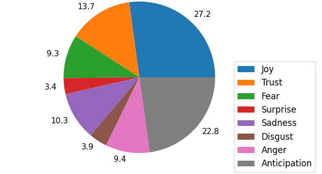
Over the course of the first few thousand annotations, it became clear that two emotion leaves were particularly overrepresented, namely “joy” and “anticipation”, respectively accounting for $35.9$% and $23.0$% of all annotations by the time of Run 9. In an attempt to counter this, we came up with the following system.

Besides the “keep/reject” CNN, we trained a second CNN to predict the Emo8 label. We then first computed all “keep/reject” predictions for all images in the corpus, and followed this up by predicting Emo8 labels for all “keep”-labeled images. Upon starting the annotation server, these predictions are loaded into memory. When selecting an image to show to a user, first an emotion label is chosen, with odds inversely proportional to the number of images that were tagged (by the CNN) with a certain label. Second, out of all images tagged with this label, one that had not previously been annotated by an annotator would be chosen. The CNN used to make the predictions was retrained at several steps along the annotation gathering process. Using this system, we managed to decrease “joy” down to $28.4$%, and up “sadness” from $6.3$% to $10.5$%.

2.3.3 Annotator Grading and Annotator Overlap

To assess the reliability of annotators, we used a set of 5 fixed images, referred to as “fixed overlap images”, chosen specifically for being unambiguous. For each image, a default annotation was defined consisting of the “keep/reject” choice (4 keeps, 1 reject), Valence (value range), Arousal (value range) and Emotion (emotion leaf). This results in 4 datapoints per image, or 20 datapoints in total. Annotators’ submissions for these images were compared to the reference, earning 1/20 point per matching datapoint, resulting in a final “overlap score” $s\in[0,1]$. Users with $s>=0.8$ were automatically accepted. An alternative score $s_{alt}$ was computed which ignored those overlap images whose reference value was “keep”, but were annotated as “reject”. The reason for this is that it quickly became clear that despite the system providing a “Skip” option in case users rather not annotate a certain image, some chose to “reject” these images instead. Also, one of the “keep” images shows a bit of text, which users were instructed to reject. Some users were more strict than others in applying this rule.

We defined a system parameter $p_{R}$ that controls when overlap images (i.e., images already annotated by others) are shown to users. For each new image request, an overlap image is served with probability $p_{R}$, starting with the 5 fixed overlap images, in a fixed sequence. Once these are annotated, the system serves other already annotated images. At first, these were randomly chosen from all annotated images, but this resulted in too many images with only 2 annotations. Hence, we created a process that limits the pool of images to choose from, and attempts to strive for 5 annotations per overlap image. Using this system, we obtained a dataset with 80.9/19.1 split single label/multi-label annotations.

A small negative correlation manifests between the task completion time and the annotator score (SpearmanR$=-0.122$, $p=0.002$ for $s$, SpearmanR$=-0.086$, $p=0.029$ for $s_{alt}$).

2.4 Statistics and Observations

This section presents statistics for the 8 leaves of PWoE. Statistics for the full 24 emotions can be found in §A.6.

The distribution of annotations per emotion leaf is depicted in Figure 4. As mentioned in §2.3.2, an imbalance is obvious, with in particular “joy” and “anticipation” being overrepresented, and “surprise” and “disgust” heavily underrepresented, despite our added balancing mechanism. This observation agrees with popular facial expression datasets, such as FER2013 (Goodfellow et al., 2015) (only 600 “disgust” images versus nearly 5,000 for other Ekman’s 6 labels) and AffectNet (Mollahosseini et al., 2019) (134,915 “happy” faces, 25,959 “sad” faces, 14,590 “surprise” faces, 4,303 “disgust” faces). Although EMOTIC (Kosti et al., 2019) uses custom emotion labels, making a one-to-one comparison more difficult, it is also heavily skewed towards positive labels (top 3: “engagement”, “happiness” and “anticipation”; bottom 3: “aversion”, “pain” and “embarassement”). Compared to these other datasets, ours exhibits less imbalance.

Figure 4: Distribution of Emotion annotations per Plutchik emotion leaf.

In Table 2, we group average annotation values for Arousal, Valence and Ambiguity. As expected, perceived “negative” emotions (“fear”, “sadness”, “disgust” and “anger”) have a negative average Valence, with the inverse being true for “positive” emotions (“joy”, “trust”). Somewhat undecided are “surprise” and “anticipation”, which can go either way. The highest Arousal values are reserved for “anger, “sadness” and “fear”. We hypothesize the unexpectedly high Arousal value for “sadness” might be due to naming this dimension “Intensity” in our interface; although a grieving person is generally considered to have low arousal, the emotion of sadness itself is felt intensely. Further analysis on the full emotion set reported in §A.6 verifies that also at this more fine-grained level, annotations conform to expectations, with Arousal levels increasing along with the intensity level of the PWoE ring, and Valence levels analogously increasing for “positive” and decreasing for “negative” emotions.

Table 2: Average annotation values for Arousal, Valence and Ambiguity per Plutchik emotion leaf. Format $x^{y}$: $x$ = average, $y$ = standard deviation.

	Joy	Trust	Fear	Surprise	Sadness	Disgust	Anger	Anticipation
Nb.	$7026$	$3549$	$2401$	$888$	$2665$	$1000$	$2439$	$5901$
Arousal	$2.96^{0.96}$	$2.57^{1.09}$	$3.24^{1.24}$	$2.57^{1.41}$	$3.42^{1.29}$	$2.44^{1.23}$	$3.59^{1.17}$	$2.46^{1.21}$
Valence	$1.90^{0.96}$	$1.41^{1.09}$	$-1.34^{1.24}$	$0.48^{1.41}$	$-1.57^{1.29}$	$-0.88^{1.23}$	$-1.58^{1.17}$	$0.56^{1.21}$
Ambiguity	$1.58^{1.66}$	$1.88^{1.64}$	$2.09^{1.61}$	$2.39^{1.68}$	$1.84^{1.66}$	$2.22^{1.65}$	$1.99^{1.63}$	$2.15^{1.61}$

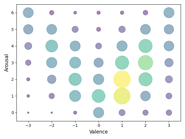
Figure 5 shows the association between Arousal and Valence annotations. Not surprisingly, these are heavily related, with higher Arousal values showing a clear collinearity with the extremes of the Valence range.

Figure 5: Association between Valence and Arousal values. The bigger the size of the disc, the more often the pair of (Valence, Arousal) annotations appears in the dataset.

3 Baseline Model Results

Baseline results are obtained by applying transfer learning to popular ImageNet-based ANN architectures AlexNet (Krizhevsky et al., 2017), VGG16 and 19 (Simonyan & Zisserman, 2015), ResNet 18, 34, 50 and 101 (He et al., 2016) and Densenet 121 and 161 (Huang et al., 2017). For each, we use the default PyTorch implementations and weights, and replace the last layer with a new output layer that matches the chosen task (see below). Only this last layer is trained. We do the same experiment for some of these same architectures that were trained from scratch on the Places365 dataset (Zhou et al., 2017). Finally, we also consider EmoNet (Kragel et al., 2019), a model for labeling images with one out of 20 custom emotion labels, reflecting the emotion elicited in the observer, obtained by applying transfer learning to AlexNet and trained on a private database. In this case, we first process the image with EmoNet, and then send the resulting 20-feature vector through a new linear layer. We use the official Places365 PyTorch models, and the EmoNet PyTorch port by on of the authors.

Figure 6: Test data baseline classification performance on the Emo8, Arousal3 and Valence3 tasks for all considered models. Metrics are: Weighted F1 (W.F1) and Average Precision (AP). The starting learning rate and loss corresponding to each model are displayed above the training bars. CE = CrossEntropyLoss, UCE = UnbalancedCrossEntropyLoss, p365 = model trained on Places365 dataset.

We distinguish three classification tasks:

• Emo8 classification: predict one of the 8 primary emotions defined by the emotion leaves of PWoE.

• Arousal3 classification: we split the $0$–$6$ range of arousal annotations into 3 groups: $[0,1]$ or low arousal, $[2,3,4]$ or medium arousal, and $[5,6]$ or high arousal, and use these groups as target classes.

• Valence3 classification: we split the $-3$–$3$ range of arousal annotations into 3 groups: $[-3,-2]$ or negative valence, $[-1,0,1]$ or neutral valence, and $[2,3]$ or positive valence, and use these groups as target classes.

For each task, and each model, we trained 10 models per starting learning rate $\mbox{lr}_{0}\in[0.1,0.01,0.001,0.0001]$, and per loss function $\mbox{lf}\in[\mbox{CrossEntropyLoss},\mbox{UnbalancedCrossEntropyLoss}]$. UnbalancedCrossEntropyLoss ($l_{\mbox{\tiny{UCE}}}$) is a novel loss, and extension of the traditional CrossEntropyLoss, that we created to allow to give different weights to different misclassifications. E.g., it allows to penalize classifying a “low arousal” as a “high arousal” image heavier than classifying it as “medium arousal”. It is defined as

$$l_{\mbox{\tiny{UCE}}}=\begin{cases}w_{t}\log{p_{t}}&t=h\\ w_{t}\log{p_{t}}+w_{t,h}\log{1-p_{h}}&t\neq h\end{cases}$$ (1)

with $t$ the target class with predicted probability $p_{t}$, $h$ the class with the highest predicted probability $p_{h}$, $w_{t}$ the weight of the target class, and $w_{t,h}$ the weight for misclassifying a sample of class $t$ as class $h$. In case $t=h$, this reverts to regular CrossEntropyLoss. A thorough description of how we determined the off-diagonal weights is contained in §A.7. Only results for the $(\mbox{lr}_{0},\mbox{lf})$-combination yielding the best performance are reported.

Preprocessing for ImageNet models consisted in scaling images to an 800x600 resolution, keeping the original ratio and centering and padding with black borders where necessary, followed by normalization. For Places365 and EmoNet models, we followed the preprocessing steps described in the respective papers.

All experiments use Adam loss with default PyTorch parameter values, and the custom lr update rule:

$$\mbox{lr}_{e}=\frac{\mbox{lr}_{0}}{\sqrt{(e//3)+1}},$$ (2)

with $\mbox{lr}_{e}$ the learning rate at epoch $e$. By virtue of the floor division ($//$), this means we update the learning rate once every 3 epochs. Data was randomly split 80/20 train/test, making sure that each Emo8 emotion was also split according to this same rule.

Reported metrics are Average Precision (AP)—as computed using the scikit-learn package—and Weighted F1 (W.F1), i.e., the weighted average of the F1 scores per class, weighted by the number of samples per class. Training stopped when either the epoch with the best loss or the best W.F1 score on the test set lies 6 epochs behind the current epoch, or 250 epochs were reached, with the corresponding best model put forward as the final trained model.

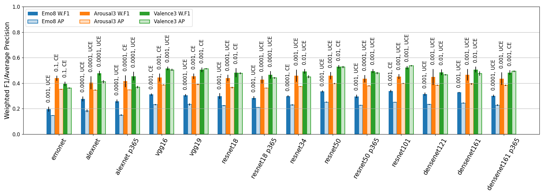
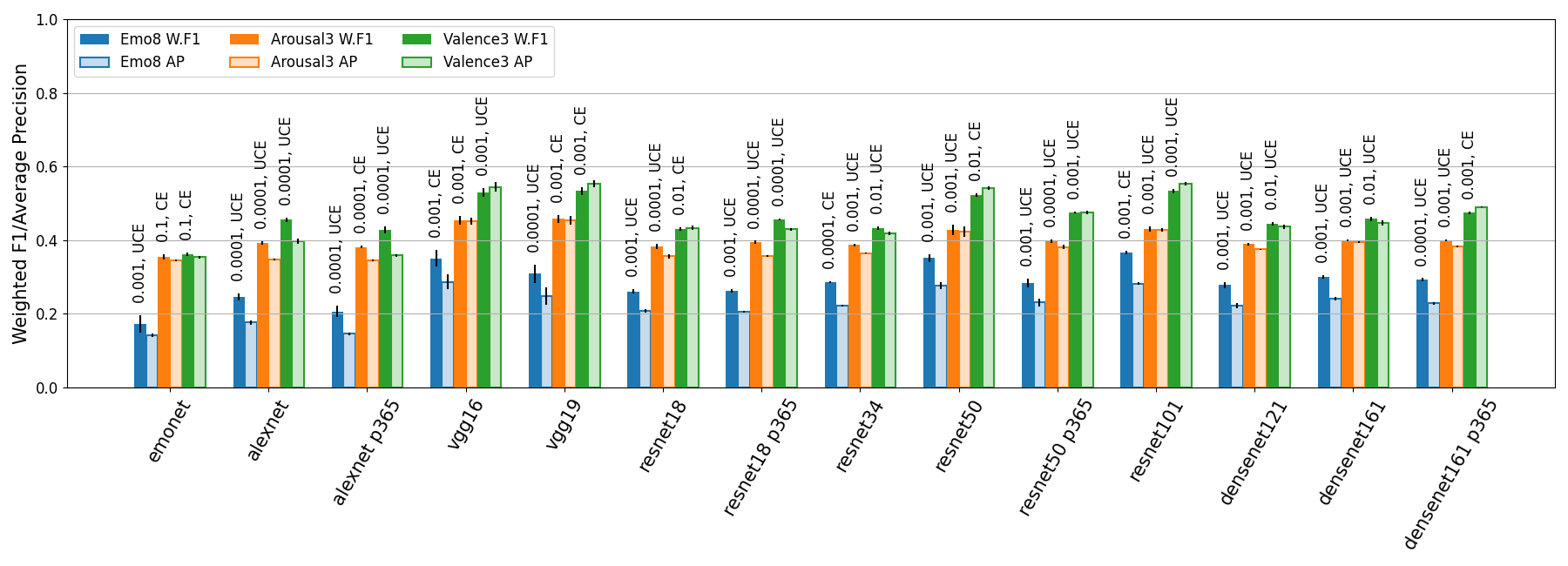
All our experiments were implemented in Python using PyTorch, and split over an Intel Xeon W-2145 workstation with 32GB RAM and two nVidia GeForce RTX 3060 GPU’s with 12GB VRAM, and an Intel i7-12800HX laptop with 32GB RAM and an nVidia GeForce RTX 3060 Laptop GPU with 12GB VRAM. Test results are plotted in Figure 6, with the graph for train data, and tables containing the numerical results grouped in §A.8. In order to speed up training, we buffered model activations whenever possible.

Figure 7: Results on test data for extensions beyond the ImageNet baseline by applying late fusion with Facial Emotion Recognition predictions (OIToFER), EmoNet predictions (EmoNet) and Places365 (P365) predictions or features. For all models, predictions on the dataset are concatenated and sent through a linear layer, except when ‘(f)’ is shown, indicating model features are concatenated.

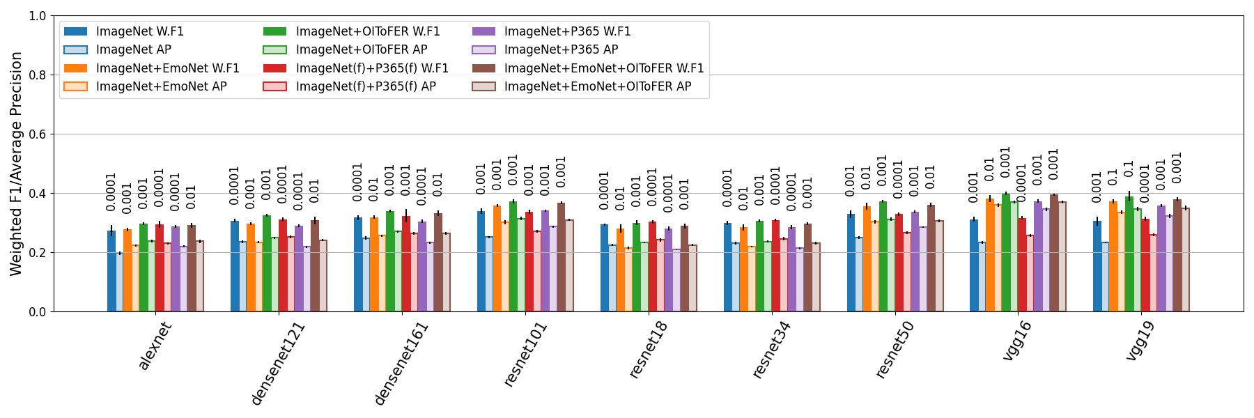
Apparent from these results is that these are hard problems. ImageNet-trained models slightly outpeform their Places365-trained counterparts. This suggests that the natural object features extracted from the ImageNet dataset are more salient toward emotion recognition than are places-related features. In 30 out of 42 cases, our UnbalancedCrossEntropy loss has the edge over regular CrossEntropyLoss. Predicting Arousal appears more difficult than predicting Valence, which aligns with lesser annotator agreement for Arousal than Valence, as analyzed in §A.5. As for the architectures, VGG is a clear winner, with ResNet second. Although twice as large, ResNet101 performs very similar to ResNet50. The larger depth of the DenseNet models does not translate in better performance. A breakdown of model performance per Emo8, Arousal3 and Valence3 class can be found in §A.8.

4 Beyond the Baseline

To build upon the baseline established in §3, we build multi-stream models by applying late fusion, a popular technique (Kosti et al., 2019; Mittal et al., 2020; Thuseethan et al., 2022; Yang et al., 2022). This section reports results for Emo8 classification; the analogous discussion for Arousal3 and Valence3 can be found in §A.9.

We consider the following streams for combinations:

• ImageNet predictions: for each considered architecture, we trained an Emo8 model, and took the predictions from this model as an 8-feature vector.

• ImageNet features: we take the model features from the penultimate layer. Vector size depends on the architecture.

• EmoNet predictions: applying the model gives us a 20-feature vector (see §3).

• YoLo v3 trained on Open Images + Facial Emotion Recognition (OIToFER): we apply YoLo v3 (Redmon & Farhadi, 2018) to each image, and extract the detected “Human face” regions with probablity $p>0.005$. We then apply the FER2013-trained ResNet18 model by X. Yuan to the extracted faces, resulting in a 7-feature vector per face. We generate two 7-feature vectors from this, one containing the vector averages, the other the standard deviations, and concatenate both to obtain a final 14-feature vector.

• Places365 ResNet18 predictions: applying the ResNet18 model trained on the Places365 dataset gives us a 365 feature vector per image.

• Places365 ResNet18 features: we take the model activations from the penultimate layer, giving us a 512-feature vector.

The experimental setup is identical to §3, except that for time considerations, we only consider CrossEntropyLoss.

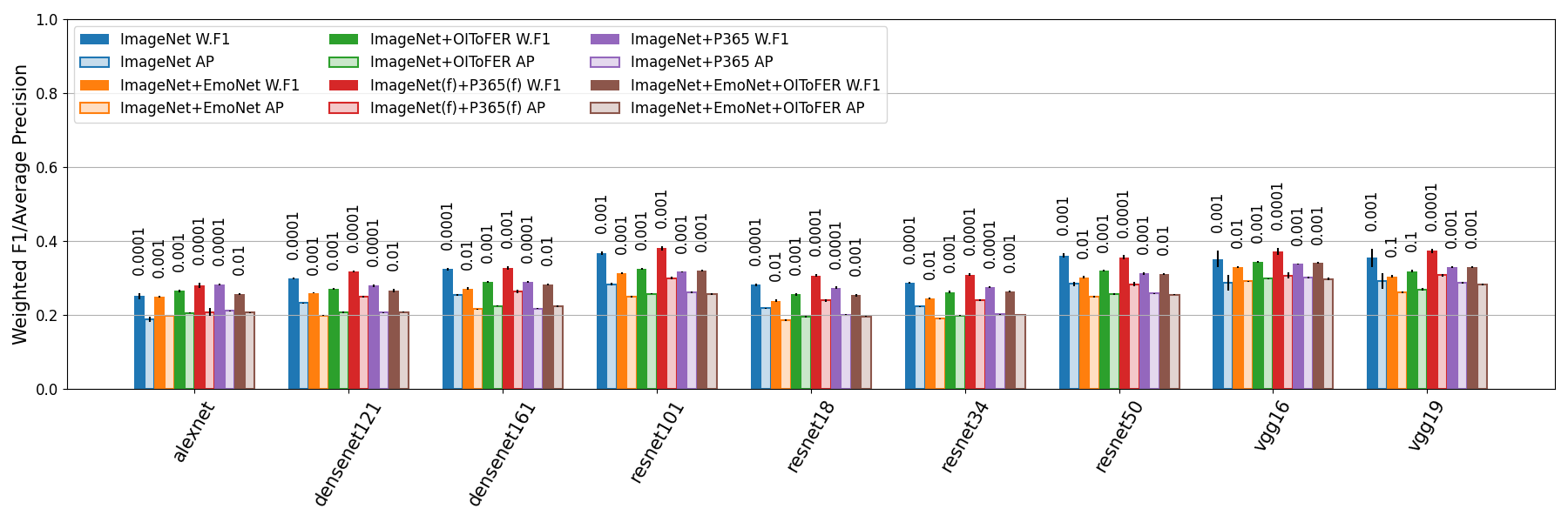
The test results for Emo8 classification are shown in Figure 7. Train results, as well as numerical test results for the Baseline+OIToFER models, are included in §A.9. A first observation is that improving upon the baseline appears non-trivial; except for VGG16 and 19, the obtained gains are modest. Second, the best gains clearly come from adding facial emotion features. Third, even though adding EmoNet and OIToFER features separately has a positive effect, adding both together does not result in a compounded improvement. Fourth, the added dimensionality of concatening features instead of predictions in the case of Places365 does not result in markedly different results, in some cases even leading to worse results. Fifth, despite EmoNet being the worst performer on its own, adding it has a beneficial effect, suggesting the model captures different salient information than the standard ImageNet networks.

5 Conclusion

We present FindingEmo, a dataset of 25k image annotations for Emotion Recognition that goes beyond the traditional focus on faces or single individuals, and is the first to target higher-order social cognition. The dataset creation process has been discussed in detail, and the annotations have been shown to align with expectations. Baseline results are presented for Emotion, Arousal and Valence prediction, as well as first steps to go beyond the baseline. These results show the dataset to be complex, and the tasks hard. Our annotation interface and code for model training are openly available.

Appendix A Appendix

A.1 Copy of the Annotator Instructions

Welcome

It is recommended to set your browser to “full-screen” mode. Typically, this mode can be toggled by using the ‘F11’ key.

This interface was designed for screen resolutions with a width of 1920 pixels. In case your screen has a higher/lower resolution, the interface should automatically resize itself so as to fully fit on your screen, but this might come at the price of reduced image sharpness.

Thank you for your willingness to participate in this annotation task!

In this experiment, you will be expected to annotate 50 “good” images, i.e., annotated as “Keep”, after which you will receive a URL that will direct you to the Prolific completion page for this task. Please take the time to read these annotation instructions before continuing.

Note that if for any reason you get logged out at some point, you should be able to log back in using the same URL provided to you by Prolific, and pick up right where you left.

We want to build a database of photographs with an emotional content. You will be shown randomly selected images from a large corpus, and we ask you to evaluate photographs regarding 2 consecutive issues.

First, regardless of the emotional content, all photographs should adhere to the following criteria:

• Each photograph must display a realistic situation, e.g., no drawings, no watermark, no fantasy content (i.e., digitally manipulated photos), no horror, etc.

• The formal quality of the photograph should be sufficient, i.e., no fuzzy/blurry photographs.

• Each picture must display at least 2 people that are clearly visible. Alternatively, if only one person is shown, but this person is clearly a part of a larger context, the image can also be suitable.

• The main feature of the photograph must not consist of a textual element. For instance, if a cardboard displaying ‘stop racism’ is a central feature of the picture, the picture is not suitable.

If an image does not adhere to each of these criteria, or you are not certain, please rate it as not suitable by choosing the “Reject” option. Else, mark it as “Keep”, in which case all other dimensions, except for “tags”, need to be annotated before you can proceed! Even if you want to keep the default value of a slider, you still need to click the slider first.

Images can further be described by a number of tags:

• Bad quality photo: when a picture is too blocky/blurry.

• Copyright: a copyright, contrary to a watermark, is not repeated but appears only once. Typically, this leads to the picture being rejected, unless possibly the copyright is only small in size and could be cropped out without losing the essence of the picture.

• Watermark: a watermark is a specific pattern, typically containing the name of the copyright holder, that is repeated over an entire image.

• No interaction: the people in the picture don’t have a direct interaction.

• No people: the picture does not depict any people.

• Text: the image contains a lot of text, either typeset on top of it, or present on, e.g., banners held by subjects depicted in the picture. If the text is typeset, this is disqualifying (i.e., the picture is rejected). If the text is present in the picture itself, it is disqualifying if it is too prominent. Use your own discretion to determine what is “too prominent” and what is not. A good rule of thumb is: if your attention is immediately drawn to the textual elements when viewing the picture, then it is too prominent and the picture is disqualified.

• Not Applicable: typically used for images that are actually a collage of more than one photo, or that are rejected but don’t fit any of the other tags.

If a photograph is not rated as suitable (i.e., “Reject”), no further assessment is required; click “Save” to proceed to the next paragraph. Else, for “Keep” or “Uncertain” photos, you are also expected to annotate the age group of the main participants in the picture. These labels are of course not clear cut; feel free to use your own discretion as to which label applies best.

Second, we want you to focus on the emotional labelling of the photographs. Concretely, we ask you to annotate the image on a number of dimensions

We ask you to indicate the emotional characteristic of the ENTIRE SCENE displayed in the photograph, independent of your own political/religious/sexual orientation. So a black lives matter protest is typically negative (= the participants are not happy) independent of whether you support BLM. Specifically, we ask you to rate the valence (“Negative/Positive”) of the overall emotional gist of the photograph on a 7-point Likert scale from negative (-3) over neutral (0) to positive (+3), and also the intensity, ranging from not intense at all (0) to very intense (6) by using the appropriate sliders.

We also ask to indicate an emotional label by means of a mouse click on an emotion wheel called “Plutchik’s Wheel of Emotions”. If you can’t find the perfect emotional label then you choose the ‘next best thing’, i.e., the one that reflects it most. In case no particular emotion fits, i.e., the participants all display a neutral expression, you can opt to select no emotion, although such cases are expected to be rare. For a more detailed description of each emotion depicted in this wheel, see, e.g., https://www.6seconds.org/2020/08/11/plutchik-wheel-emotions/. Additional info for each emotion will be displayed when hovering over its corresponding cell.

Please also rate how straightforward the emotional content that is exhibited by the entire photograph is using the scale indicated with “Ambiguity”. For instance, if there are approximately as much emotionally positive as emotionally negative cues in the photograph, the emotional content would not be clear (6), while only positive cues or only negative cues would result in a very high clarity (0).

Finally, the options under the “Deciding factor(s) for emotion” header ask which aspects of the photo influenced you most when assessing the emotion, i.e., facial expressions, bodily expressions, the type of interaction (‘Staging’) among the persons (e.g., fighting, dancing, talking), type of context (e.g., wedding, funeral, protest, etc.), objects in the photograph (e.g., gun, chocolate) or a possible conflict between context and person(s) (i.e., somebody exuberantly laughing at a funeral). If none of these apply, and/or the emotion is rather neutral, the “Neutral” tag can be used, although just as for the emotion case, we expect these occasions to be rare.

If for some reason you would rather not annotate the current image being served to you, you can press the “Skip” button to be served a new picture and have the annotation interface be reset, without your current settings being saved.

If on the other hand you are happy with your current annotation, press “Save” to let it be saved and move on to the next image. If this button is greyed out, this means you have not yet annotated all necessary dimensions. Once you have reached the required number of annotations, you will automatically get to see the URL that will direct you to the Prolific completion page for this task.

At the top of this screen, you can see your annotation statistics: “Rejected/Accepted” = how many images you marked “Reject” and “Keep” respectively, and “Left” = number of “Keep” images left to annotate.

You can always check these instructions again whilst annotating by clicking the -icon next to each criterium. (Click once more to close the infobox again.)

A.2 Annotation Interface

A screenshot of the annotation interface is shown in Figure LABEL:fig:ann_interface.

A.3 Task Duration Analysis

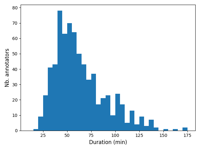
A histogram of time taken per annotator to complete the task is shown in Figure 8. These are the durations as reported by Prolific. An important remark to make is that for Prolific users, the clock starts ticking once they subscribe to a job. By default, per the Prolific rules, for a job expected to take 1h users are allowed a maximum of 140 minutes to complete the job. It appears that many users subscribe to a job, and then leave their browser tab open for a while before starting the job proper. (Some never start, leading to a time-out.) Taking this into account, the shown distribution is a “pessimistic” picture, including many idled minutes. The average time taken per user, including users that were ultimately filtered out of the dataset, was 64 $\pm$ 27 minutes. With all of the above in mind, we conclude our alloted time was fair.

Figure 8: Distribution of minutes taken to complete the task. The plot does not include 7 outliers.

A.4 Annotator Statistics

Annotations were collected from 655 annotators. Prolific provided us with anonymized personal data, except for 1 user. Not all datapoints are available for all users.

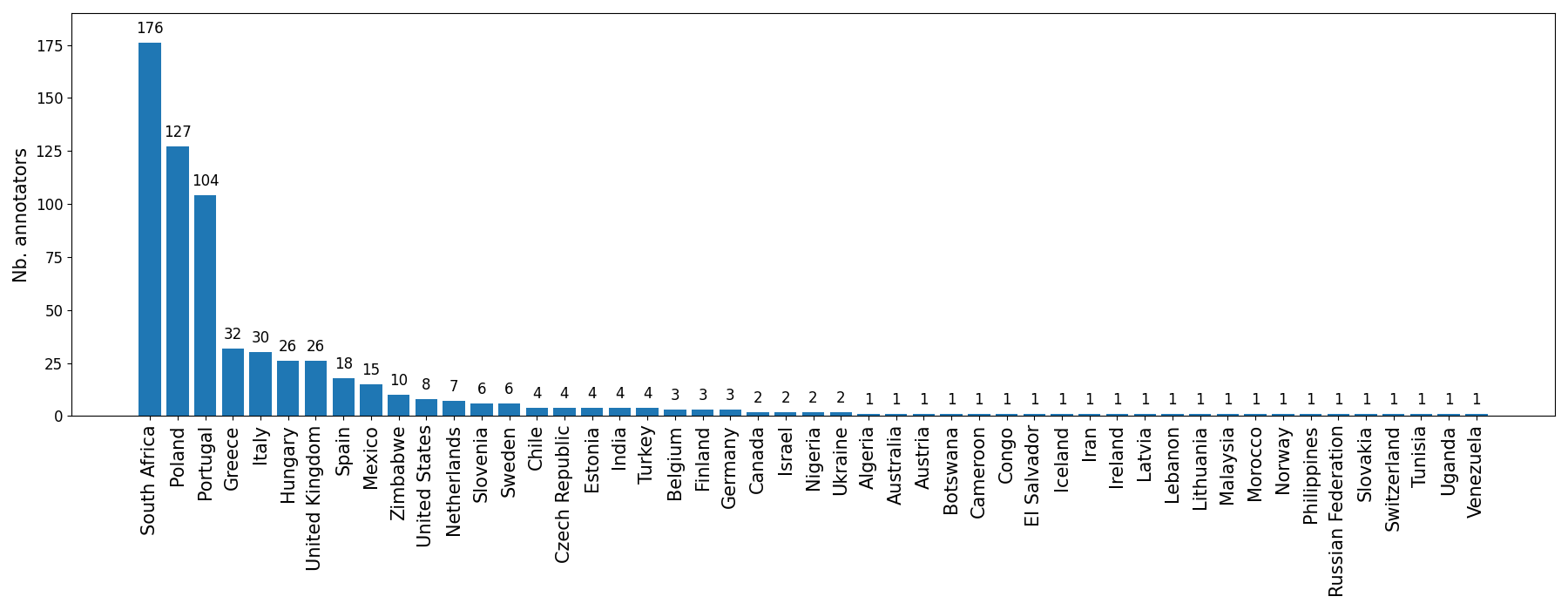
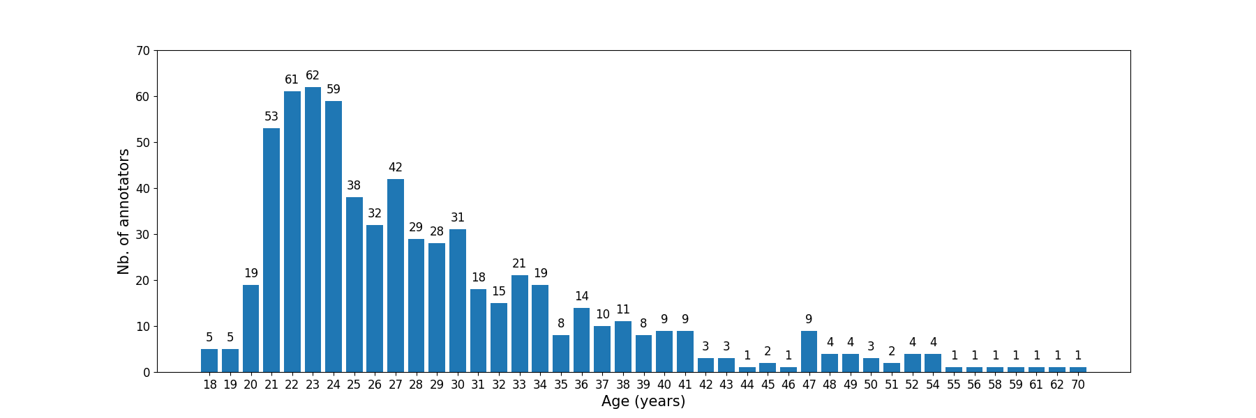
Of the annotators, 337 are male, 317 are female, and 1 unknown. 651 annotators were spread over 49 countries, with country for the remaining 4 unknown. Most popular were South Africa (176 annotators), Poland (127 annotators) and Portugal (104 annotators). From there, numbers drop rapidly, with follow-up Greece accounting for only 32 annotators. The full distribution of annotators per country is shown in Figure 9. The age distribution of the 653 users who shared that info is shown in Figure 10, indicating a large bias towards the early 20’s.

Figure 9: Distribution of country of origin for 651 annotators.

Figure 10: Distribution of age for 653 annotators.

A.5 Inter-annotator Agreement

Recall from §2.1 that we hold a private set of 1525 images that have each been annotated by multiple users, amounting to a combined 6115 annotations. Table 3 shows how many images have been annotated by $N$ different annotators. Of these, 1294 images have a majority of “Keep” annotations, 137 are mainly “Reject” and 94 are undecided.

Table 3: Number of images (“# imgs.”) that have been annotated by $N$ different annotators (“# ants.”).

# ants.	2	3	4	5	6	7	8
# imgs.	245	328	283	524	127	17	1

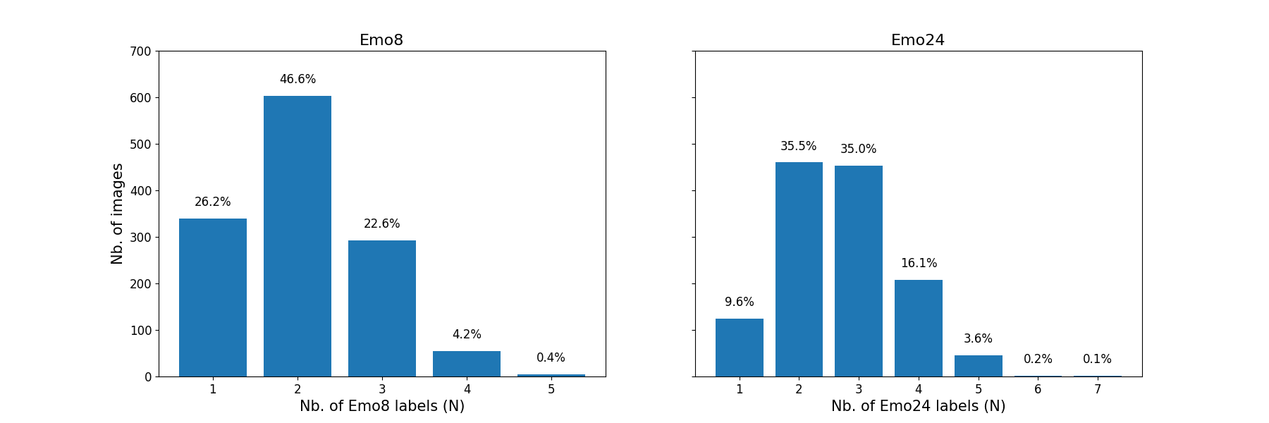
Focusing on the 1294 “Keep” images, Figure 11 shows how many images have been annotated with $N$ different emotion labels, both for Emo8 and Emo24 labels. For 26.2% of images, all annotators chose the same emotion leaf, and 46.6% were annotated with 2 different Emo8 labels. For the finegrained Emo24 labels, 80.1% of images have been annotated with a maximum of 3 different labels.

Figure 11: Histograms showing the number of images with $N$ different Emo8 and Emo24 labels. The y-axis is shared between both plots.

Figure 12: Plutchik’s Wheel of Emotions: ordinals of emotions. The outer numbers represent the ordinal of the leaf, the numbers within the upper central leaf the ordinals of the emotions within a leaf. E.g., “joy” = 0.66, and “boredom” = 5.33. The distance between them then becomes 3.33, being the sum of the distance between the leaves (3) and the “intra-leaf” distance (0.33).

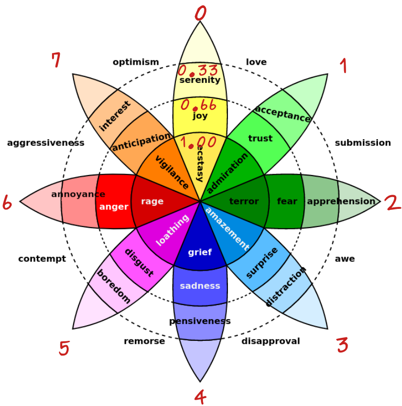
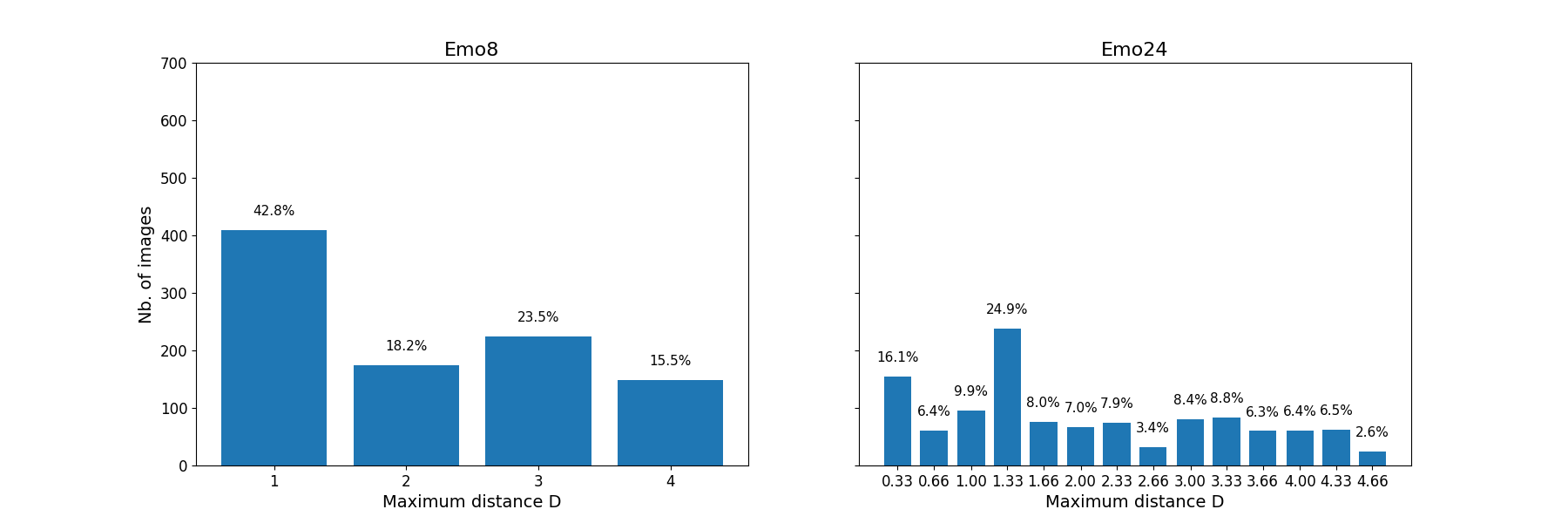
Turning to the question of how different the separate emotion labels for a same image are, Figure 11 shows the distribution of maximum distance between labels, for images annotated with more than one label. The distances for 24 emotions are computed by also giving an ordinal to each emotion within a leaf, as shown in Figure 12. No less than 42.8% of the times an image has been annotated with more than one Emo8 label, those labels represent adjacent emotion leaves, while in 15.5% of the cases they represented opposite leaves.

Figure 13: Histograms showing the number of images with a maximum difference $D$ between their Emo8 and Emo24 labels, for images annotated with more than one label. The y-axis is shared between both plots.

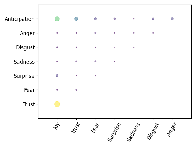
To get a better idea of what Emo8 labels often appear together, we focused on images with 2 Emo8 labels, and plotted how often each emotion pair occurs. The result is shown in Figure 14, demonstrating the pairs (“Joy”, “Anticipation”), (“Joy”, “Trust) and (“Aniticipation”, “Trust”) make up the bulk of the pairs. As for opposite emotions, the pairs (“Anticipation”, “Surprise”) and (“Anger”, “Fear”) appear markedly more ofthen than (“Joy”, “Sadness”) and (“Disgust”, “Trust”).

Figure 14: Prevalence of Emo8 label pairs for images annotated with 2 labels. The bigger the size of the disc, the more often the pair appears in the dataset.

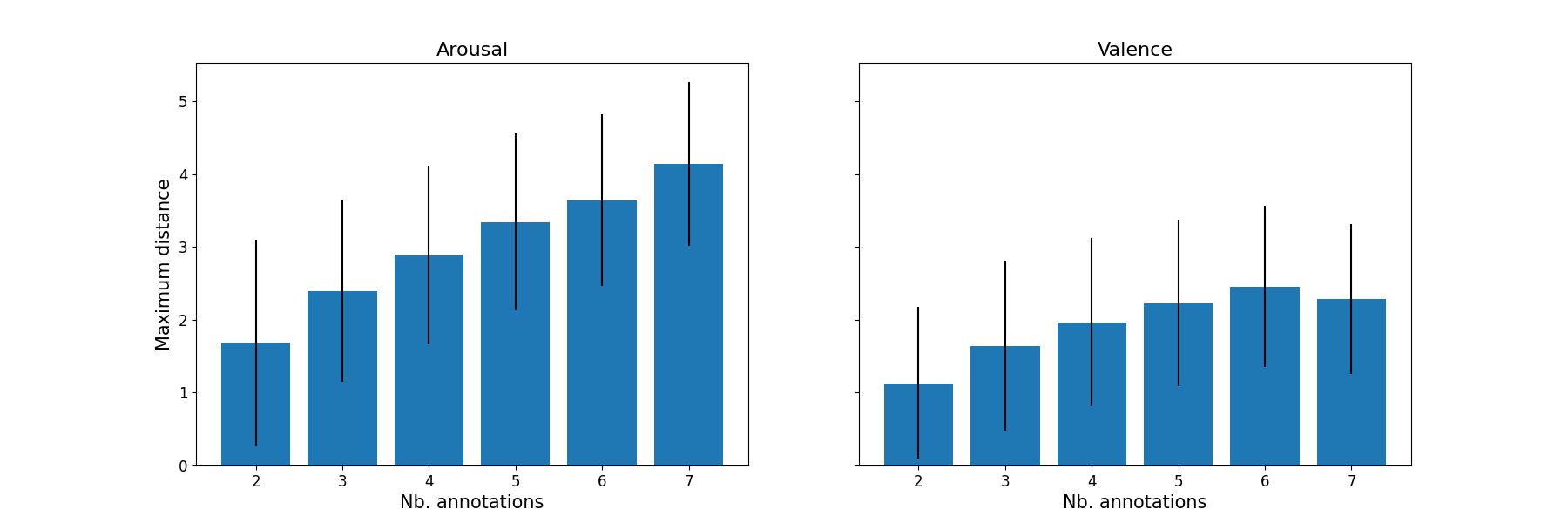
To analyze the Arousal and Valence values, we compute the maximum distance between annotated values for both dimensions over all “keep” images. For Arousal, the average maximum distance is 2.7 $\pm$ 1.4, while for Valence this is 1.8 $\pm$ 1.2. This suggests that people agree much more on the Valence dimension, than they do on the Arousal dimension. This is confirmed when we compute the average maximum distance values as a function of the number of annotations for a given image, the result of which is shown in Figure 15. For Arousal, a clear increasing maximum distance trend is visible with a stable standard deviation, going from $\pm 1.75$ to more than $4$. For Valence annotations on the other hand, the maximum distance appears to plateau at close to $2$.

Figure 15: Distribution of maximum distance between Arousal and Valence annotations as a function of the number of annotations per image. The y-axis is shared between both plots.

A.6 Extra Dataset Analysis

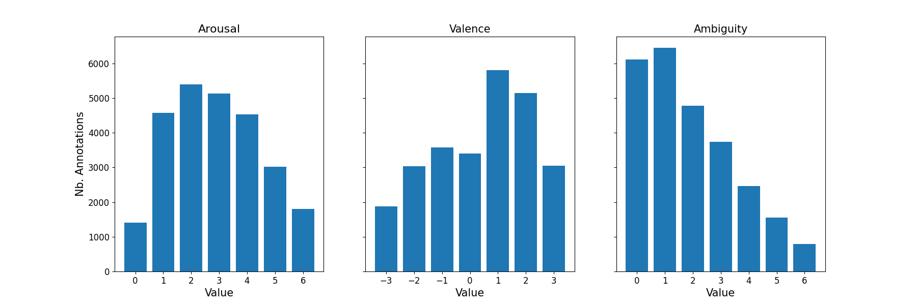
Histograms showing the distribution of Arousal, Valence and Ambiguity annotation values are depicted in Figure 16.

Figure 16: Histograms of Arousal, Valence and Ambiguity annotations. The y-axis is shared between all plots.

Annotation statistics per Emo24 emotion are collected in Table LABEL:tb:emo24_ann_stats. The table is made up of three rows, each row corresponding to a ring in Plutchik’s Wheel of Emotions, from the top row corresponding to the outer (least intense) ring, to the bottom row corresponding to the inner (most intense) ring. The annotations follow this ordering, with average Arousal annotations consistently increasing from least to most intense emotion ring. Valence annotations follow suit, either increasing for positive emotions, or decreasing for negative emotions. The sole exception to this rule is center ring “Disgust” having a slightly lower average Valence rating (-1.62) than the inner ring “Loathing” (-1.57).

A.7 UnbalancedCrossEntropyLoss

To be able to use UnbalancedCrossEntropy loss, a distance needs to be defined between each pair of output classes. For the Emo8 task, we use the shortest number of leaves between two emotions. E.g., the distance between “joy” and “surprise” is 3, and the distance between “joy” and “anger” is 2. The Arousal3 classes are ordered as [Low, Medium, High], and the distance between two classes is simply the number of steps between them. E.g., the distance between Low and High is 2. For Valence3 classes, the approach is analogous.

The class weight $w_{i}$ for class $i$ was computed according to

$$w_{i}=\frac{N}{N_{c}\cdot N_{i}},$$ (3)

with $N$ the total number of samples, $N_{c}$ the number of classes and $N_{i}$ the number of samples of class $i$.

Finally, the weight $w_{i,j}$ for misclassifying a sample from class $i$ as class $j$ was computed as

$$w_{i,j}=\frac{d_{i,j}}{1+w_{j}}\cdot w_{i},$$ (4)

with $w_{i}$ the weight for class $i$, $w_{j}$ the weight for class $j$ and $d_{i,j}$ the distance between classes $i$ and $j$.

Table LABEL:tb:baseline_cs_vs_uce compares baseline results obtained using CrossEntropyLoss vs. UnbalancedCrossEntropyLoss.

A.8 Additional Baseline Results

Baseline results for train data are depicted in Figure 17. Numerical baseline results on the train and test sets have been grouped in Tables LABEL:tb:baseline_models_train and LABEL:tb:baseline_models_test respectively. A breakdown per Emo8 for train and test sets is shown in Tables LABEL:tb:baseline_perf_per_class_train and LABEL:tb:baseline_perf_per_class_test respectively. For Arousal and Valence classes, the results are grouped in Tables LABEL:tb:baseline_aro3_val3_perf_per_class_train and LABEL:tb:baseline_aro3_val3_perf_per_class_test for train and test sets respectively. For per class results, no Average Precision scores are reported, as we did not collect these.

Figure 17: Train data baseline classification performance on the Emo8, Arousal3 and Valence3 tasks for all considered models. Metrics are: Weighted F1 (W.F1) and Average Precision (AP). The starting learning rate and loss corresponding to each model are displayed above the training bars. CE = CrossEntropyLoss, UCE = UnbalancedCrossEntropyLoss, p365 = model trained on Places365 dataset.

A.9 Additional Beyond Baseline Emo8, Arousal3 and Valence3 Results

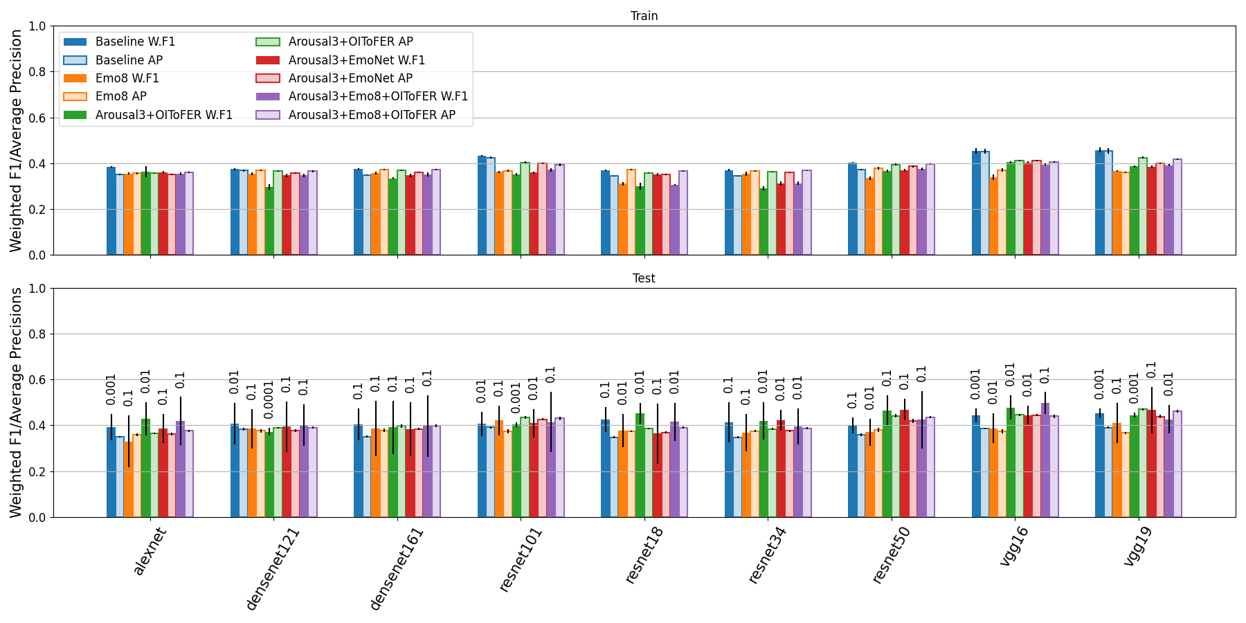
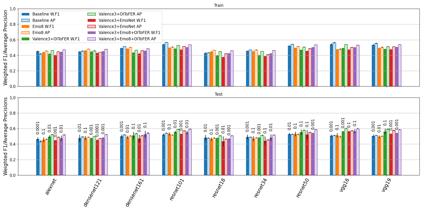
The beyond baseline Emo8 results on train data are shown in Figure 18. Barcharts depicting the beyond baseline results for the Arousal3 and Valence3 classification tasks are grouped in Figures 19 and 20 respectively.

For the Arousal3 and Valence3 tasks, we dropped experiments with Places365 models in favor of precomputed Emo8 predictions using the same model architecture. E.g., for the Arousal3 task and AlexNet architecture, we combine the 8-feature vector obtained by applying a pretrained AlexNet Emo8 classifier with the 3-feature vector obtained by applying a pretrained AlexNet Arousal3 classifier.

A numerical comparison of the baseline to the (best performing) “Baseline+OIToFER” model for all three tasks is included in Table 4. From this, it is apparent that obtainble gains are architecture-dependent, with the VGG architecture obtaining most gains and the DenseNet architecture barely improving, regardless of task. Obtained gains are highest for the Emo8 task (absolute 13.7% AP gain, or relative 59%, for VGG16), followed by the Valence3 task (absolute 9% AP, relative 17.6%, for VGG16), and lowest for the Arousal3 task (absolute 6% AP gain, relative 15.5%, for VGG16).

Remarkebly, for the Valence3 task, we obtain quasi identical test results using precomputed Emo8 predictions compared to training a dedicated model, further confirming the high correlation between Emotion and Valence. For the Arousal3 task, results are architecture dependent, with the VGG models and ResNet18 and 34 clearly benefitting from training a dedicated model.

Figure 18: Results on train data for extensions beyond the ImageNet baseline by applying late fusion with Facial Emotion Recognition predictions (OIToFER), EmoNet predictions (EmoNet) and Places365 (P365) predictions or features. For all models, predictions on the dataset are concatenated and sent through a linear layer, except when ‘(f)’ is shown, indicating model features are concatenated.

Figure 19: Arousal3 results for extensions beyond the ImageNet baseline by applying late fusion with precomputed Emo8 predictions of the same architecture (Emo8), Facial Emotion Recognition predictions (OIToFER) and EmoNet predictions (EmoNet). For all models, precomputed predictions on the dataset (Arousal3) are concatenated and sent through a linear layer

Figure 20: Valence3 results for extensions beyond the ImageNet baseline by applying late fusion with precomputed Emo8 predictions of the same architecture (Emo8), Facial Emotion Recognition predictions (OIToFER) and EmoNet predictions (EmoNet). For all models, precomputed predictions on the dataset (Valence3) are concatenated and sent through a linear layer

Table 4: Baseline vs. +OIToFER: Emo8, Arousal3 and Valence3 classification performance. Performance metrics format: $.xxx^{yy}$ should be read as average = $0.xxx$, standard deviation = $.0yy$, taken over 10 runs.

		alexnet	vgg16	vgg19	resnet18	resnet34	resnet50	resnet101	densenet121	densenet161
		Emo8
Baseline	Start LR	$0.0001$	$0.001$	$0.001$	$0.0001$	$0.0001$	$0.0001$	$0.001$	$0.0001$	$0.0001$
	Accuracy	$.271^{25}$	$.303^{10}$	$.298^{20}$	$.271^{08}$	$.293^{07}$	$.279^{09}$	$.329^{11}$	$.300^{07}$	$.308^{09}$
	F1	$.221^{10}$	$.251^{07}$	$.248^{07}$	$.232^{06}$	$.249^{07}$	$.240^{08}$	$.277^{06}$	$.252^{07}$	$.261^{08}$
	Weighted F1	$.273^{18}$	$.311^{08}$	$.305^{16}$	$.281^{07}$	$.299^{07}$	$.289^{09}$	$.339^{09}$	$.306^{06}$	$.316^{08}$
	Avg.Prec.	$.196^{06}$	$.232^{05}$	$.232^{03}$	$.215^{06}$	$.230^{04}$	$.228^{06}$	$.250^{03}$	$.235^{04}$	$.247^{05}$
+OIToFER	Start LR	$0.001$	$0.001$	$0.1$	$0.001$	$0.001$	$0.001$	$0.001$	$0.001$	$0.001$
	Accuracy	$.299^{04}$	$.390^{05}$	$.381^{20}$	$.315^{06}$	$.318^{05}$	$.366^{05}$	$.367^{07}$	$.335^{05}$	$.343^{04}$
	F1	$.243^{03}$	$.363^{05}$	$.347^{16}$	$.239^{06}$	$.243^{04}$	$.321^{04}$	$.321^{07}$	$.259^{03}$	$.278^{05}$
	Weighted F1	$.296^{04}$	$.399^{05}$	$.389^{18}$	$.299^{07}$	$.306^{05}$	$.372^{04}$	$.372^{07}$	$.325^{05}$	$.339^{04}$
	Avg.Prec.	$.237^{05}$	$.369^{05}$	$.346^{07}$	$.232^{02}$	$.236^{03}$	$.311^{05}$	$.313^{06}$	$.248^{04}$	$.269^{03}$
		Arousal3
Baseline	Start LR	$0.001$	$0.001$	$0.001$	$0.001$	$0.1$	$0.01$	$0.01$	$0.01$	$0.1$
	Accuracy	$.410^{88}$	$.440^{33}$	$.451^{26}$	$.399^{74}$	$.450^{92}$	$.425^{57}$	$.407^{58}$	$.446^{98}$	$.423^{78}$
	F1	$.342^{20}$	$.384^{10}$	$.390^{08}$	$.359^{29}$	$.334^{30}$	$.371^{17}$	$.374^{20}$	$.346^{29}$	$.349^{32}$
	Weighted F1	$.393^{58}$	$.444^{30}$	$.453^{21}$	$.387^{77}$	$.412^{88}$	$.425^{44}$	$.407^{53}$	$.407^{91}$	$.405^{69}$
	Avg.Prec.	$.349^{03}$	$.386^{04}$	$.390^{05}$	$.377^{04}$	$.348^{05}$	$.373^{06}$	$.391^{05}$	$.384^{05}$	$.351^{05}$
+OIToFER	Start LR	$0.01$	$0.01$	$0.001$	$0.01$	$0.01$	$0.1$	$0.001$	$0.0001$	$0.1$
	Accuracy	$.441^{64}$	$.474^{44}$	$.441^{10}$	$.468^{53}$	$.437^{79}$	$.476^{68}$	$.403^{09}$	$.370^{11}$	$.426^{98}$
	F1	$.357^{35}$	$.437^{26}$	$.437^{08}$	$.379^{17}$	$.367^{31}$	$.421^{29}$	$.402^{08}$	$.367^{08}$	$.361^{51}$
	Weighted F1	$.429^{74}$	$.477^{53}$	$.445^{11}$	$.452^{45}$	$.419^{82}$	$.465^{65}$	$.403^{09}$	$.372^{16}$	$.391^{16}$
	Avg.Prec.	$.365^{03}$	$.446^{05}$	$.470^{05}$	$.386^{04}$	$.384^{04}$	$.441^{08}$	$.434^{07}$	$.389^{04}$	$.397^{08}$
		Valence3
Baseline	Start LR	$0.0001$	$0.001$	$0.001$	$0.001$	$0.001$	$0.01$	$0.001$	$0.01$	$0.001$
	Accuracy	$.469^{16}$	$.509^{15}$	$.506^{17}$	$.462^{18}$	$.495^{24}$	$.485^{23}$	$.524^{12}$	$.486^{32}$	$.504^{20}$
	F1	$.466^{14}$	$.499^{08}$	$.499^{12}$	$.459^{16}$	$.486^{16}$	$.471^{13}$	$.523^{08}$	$.479^{28}$	$.501^{14}$
	Weighted F1	$.464^{22}$	$.508^{14}$	$.505^{19}$	$.457^{25}$	$.492^{27}$	$.482^{25}$	$.521^{14}$	$.477^{43}$	$.501^{22}$
	Avg.Prec.	$.434^{16}$	$.512^{08}$	$.513^{04}$	$.465^{06}$	$.489^{05}$	$.471^{06}$	$.540^{06}$	$.494^{08}$	$.519^{05}$
+OIToFER	Start LR	$0.01$	$0.001$	$0.1$	$0.001$	$0.001$	$0.1$	$0.01$	$0.001$	$0.1$
	Accuracy	$.496^{16}$	$.560^{06}$	$.566^{28}$	$.477^{05}$	$.485^{06}$	$.557^{30}$	$.555^{13}$	$.473^{06}$	$.521^{34}$
	F1	$.491^{10}$	$.559^{07}$	$.552^{23}$	$.477^{05}$	$.485^{06}$	$.545^{23}$	$.554^{10}$	$.471^{06}$	$.503^{25}$
	Weighted F1	$.496^{18}$	$.560^{06}$	$.561^{37}$	$.477^{06}$	$.484^{06}$	$.553^{34}$	$.555^{15}$	$.473^{06}$	$.511^{45}$
	Avg.Prec.	$.522^{06}$	$.602^{09}$	$.592^{08}$	$.508^{06}$	$.512^{07}$	$.578^{07}$	$.588^{06}$	$.497^{04}$	$.536^{07}$

References

- Aviezer et al. (2012) Aviezer, H., Trope, Y., and Todorov, A. Body cues, not facial expressions, discriminate between intense positive and negative emotions. Science, 338(6111):1225–1229, 2012.
- Barrett (1998) Barrett, L. F. Discrete emotions or dimensions? the role of valence focus and arousal focus. Cognition and Emotion, 12(4):579–599, 1998.
- Barrett et al. (2009) Barrett, L. F., Gendron, M., and Huang, Y.-M. Do discrete emotions exist? Philosophical Psychology, 22(4):427–437, 2009.
- Cowie et al. (2001) Cowie, R., Douglas-Cowie, E., Tsapatsoulis, N., Votsis, G., Kollias, S., Fellenz, W., and Taylor, J. Emotion recognition in human-computer interaction. IEEE Signal Processing Magazine, 18(1):32–80, 2001.
- Ekman (1970) Ekman, P. Universal facial expressions of emotion. California Mental Health Research Digest, 8(4):151–158, 1970.
- Emanuel & Eldar (2023) Emanuel, A. and Eldar, E. Emotions as computations. Neuroscience & Biobehavioral Reviews, 144:104977, 2023. ISSN 0149-7634.
- Goodfellow et al. (2015) Goodfellow, I. J., Erhan, D., Luc Carrier, P., Courville, A., Mirza, M., Hamner, B., Cukierski, W., Tang, Y., Thaler, D., Lee, D.-H., Zhou, Y., Ramaiah, C., Feng, F., Li, R., Wang, X., Athanasakis, D., Shawe-Taylor, J., Milakov, M., Park, J., Ionescu, R., Popescu, M., Grozea, C., Bergstra, J., Xie, J., Romaszko, L., Xu, B., Chuang, Z., and Bengio, Y. Challenges in representation learning: A report on three machine learning contests. Neural networks, 64:59–63, 2015. ISSN 0893-6080.
- Harmon-Jones et al. (2017) Harmon-Jones, E., Harmon-Jones, C., and Summerell, E. On the importance of both dimensional and discrete models of emotion. Behavioral Sciences, 7(4):66–, 2017. ISSN 2076-328X.
- He et al. (2015) He, K., Zhang, X., Ren, S., and Sun, J. Delving deep into rectifiers: Surpassing human-level performance on imagenet classification. arXiv.org, 2015. ISSN 2331-8422.
- He et al. (2016) He, K., Zhang, X., Ren, S., and Sun, J. Deep residual learning for image recognition. In 2016 IEEE Conference on Computer Vision and Pattern Recognition (CVPR), pp. 770–778, 2016.
- Huang et al. (2017) Huang, G., Liu, Z., Van Der Maaten, L., and Weinberger, K. Q. Densely connected convolutional networks. In 2017 IEEE Conference on Computer Vision and Pattern Recognition (CVPR), pp. 2261–2269, 2017.
- Huang et al. (2023) Huang, Z. Y., Chiang, C. C., Chen, J. H., Chen, Y. C., Chung, H. L., Cai, Y. P., and Hsu, H. C. A study on computer vision for facial emotion recognition. Scientific reports, 13(1):8425–8425, 2023. ISSN 2045-2322.
- Khare et al. (2024) Khare, S. K., Blanes-Vidal, V., Nadimi, E. S., and Acharya, U. R. Emotion recognition and artificial intelligence: A systematic review (2014–2023) and research recommendations. Information Fusion, 102:102019, 2024. ISSN 1566-2535.
- Kosti et al. (2019) Kosti, R., Alvarez, J. M., Recasens, A., and Lapedriza, A. Context based emotion recognition using emotic dataset. IEEE Transactions on Pattern Analysis and Machine Intelligence, 2019. ISSN 0162-8828, 2160-9292, 1939-3539. arXiv:2003.13401 [cs].
- Kragel et al. (2019) Kragel, P. A., Reddan, M. C., LaBar, K. S., and Wager, T. D. Emotion schemas are embedded in the human visual system. Science Advances, 5(7):eaaw4358, 2019.
- Krizhevsky et al. (2017) Krizhevsky, A., Sutskever, I., and Hinton, G. E. Imagenet classification with deep convolutional neural networks. Commun. ACM, 60(6):84–90, may 2017. ISSN 0001-0782.
- Kumfor et al. (2018) Kumfor, F., Ibañez, A., Hutchings, R., Hazelton, J. L., Hodges, J. R., and Piguet, O. Beyond the face: how context modulates emotion processing in frontotemporal dementia subtypes. Brain, 141(4):1172–1185, 01 2018. ISSN 0006-8950.
- Lee et al. (2019) Lee, J., Kim, S., Kim, S., Park, J., and Sohn, K. Context-aware emotion recognition networks. In 2019 IEEE/CVF International Conference on Computer Vision (ICCV), pp. 10142–10151, 2019.
- Lucey et al. (2010) Lucey, P., Cohn, J. F., Kanade, T., Saragih, J., Ambadar, Z., and Matthews, I. The extended cohn-kanade dataset (ck+): A complete dataset for action unit and emotion-specified expression. In 2010 IEEE Computer Society Conference on Computer Vision and Pattern Recognition - Workshops, pp. 94–101. IEEE, 2010. ISBN 9781424470297.
- Lyons et al. (1998) Lyons, M., Akamatsu, S., Kamachi, M., and Gyoba, J. Coding facial expressions with gabor wavelets. In Proceedings - 3rd IEEE International Conference on Automatic Face and Gesture Recognition, FG 1998, pp. 200–205. IEEE, 1998. ISBN 0818683449.
- McKinney et al. (2020) McKinney, S. M., Sieniek, M., Godbole, V., Godwin, J., Antropova, N., Ashrafian, H., Back, T., Chesus, M., Corrado, G. C., Darzi, A., Etemadi, M., Garcia-Vicente, F., Gilbert, F. J., Halling-Brown, M., Hassabis, D., Jansen, S., Karthikesalingam, A., Kelly, C. J., King, D., Ledsam, J. R., Melnick, D., Mostofi, H., Peng, L., Reicher, J. J., Romera-Paredes, B., Sidebottom, R., Suleyman, M., Tse, D., Young, K. C., De Fauw, J., and Shetty, S. International evaluation of an ai system for breast cancer screening. Nature (London), 577(7788):89–94, 2020. ISSN 0028-0836.
- Mehrabian (1996) Mehrabian, A. Pleasure-arousal-dominance: A general framework for describing and measuring individual differences in temperament. Current Psychology: A Journal for Diverse Perspectives on Diverse Psychological Issues, 14(4):261–292, 1996.
- Mittal et al. (2020) Mittal, T., Guhan, P., Bhattacharya, U., Chandra, R., Bera, A., and Manocha, D. Emoticon: Context-aware multimodal emotion recognition using frege’s principle. In 2020 IEEE/CVF Conference on Computer Vision and Pattern Recognition (CVPR), 2020.
- Mollahosseini et al. (2019) Mollahosseini, A., Hasani, B., and Mahoor, M. H. Affectnet: A database for facial expression, valence, and arousal computing in the wild. IEEE transactions on affective computing, 10(1):18–31, 2019. ISSN 1949-3045.
- Picard (1997) Picard, R. W. Affective computing. MIT Press, Cambridge, Mass, 1997. ISBN 0-585-00319-X.
- Plutchik (1980) Plutchik, R. A general psychoevolutionary theory of emotion. 1980.
- Redmon & Farhadi (2018) Redmon, J. and Farhadi, A. Yolov3: An incremental improvement. ArXiv, abs/1804.02767, 2018.
- Russell (1980) Russell, J. A. A circumplex model of affect. Journal of personality and social psychology, 39(6):1161–1178, 1980. ISSN 0022-3514.
- Scherer (2005) Scherer, K. R. What are emotions? and how can they be measured? SOCIAL SCIENCE INFORMATION SUR LES SCIENCES SOCIALES, 44(4):695–729, 2005. ISSN 0539-0184.
- Simonyan & Zisserman (2015) Simonyan, K. and Zisserman, A. Very deep convolutional networks for large-scale image recognition. In Bengio, Y. and LeCun, Y. (eds.), 3rd International Conference on Learning Representations, ICLR 2015, San Diego, CA, USA, May 7-9, 2015, Conference Track Proceedings, 2015.
- Spezialetti et al. (2020) Spezialetti, M., Placidi, G., and Rossi, S. Emotion recognition for human-robot interaction: Recent advances and future perspectives. Frontiers in Robotics and AI, 7, 2020. ISSN 2296-9144.
- Thuseethan et al. (2022) Thuseethan, S., Rajasegarar, S., and Yearwood, J. Emosec: Emotion recognition from scene context. Neurocomputing, 492:174–187, 2022. ISSN 0925-2312.
- Tian et al. (2001) Tian, Y.-I., Kanade, T., and Cohn, J. Recognizing action units for facial expression analysis. IEEE transactions on pattern analysis and machine intelligence, 23(2):97–115, 2001. ISSN 0162-8828.
- Yang et al. (2022) Yang, D., Huang, S., Wang, S., Liu, Y., Zhai, P., Su, L., Li, M., and Zhang, L. Emotion recognition for multiple context awareness. In Avidan, S., Brostow, G., Cissé, M., Farinella, G. M., and Hassner, T. (eds.), Computer Vision – ECCV 2022, pp. 144–162, Cham, 2022. Springer Nature Switzerland. ISBN 978-3-031-19836-6.
- Zhang et al. (2018) Zhang, F., Zhang, T., Mao, Q., and Xu, C. Joint pose and expression modeling for facial expression recognition. In 2018 IEEE/CVF Conference on Computer Vision and Pattern Recognition, pp. 3359–3368. IEEE, 2018. ISBN 9781538664209.
- Zhang et al. (2012) Zhang, S., Zhao, X., and Lei, B. Robust facial expression recognition via compressive sensing. Sensors (Basel, Switzerland), 12(3):3747–3761, 2012. ISSN 1424-8220.
- Zhang et al. (2021) Zhang, S., Huang, Z., Paudel, D. P., and Van Gool, L. Facial emotion recognition with noisy multi-task annotations. IEEE, 2021. ISBN 978-1-6654-0477-8.
- Zhao & Pietikainen (2007) Zhao, G. and Pietikainen, M. Dynamic texture recognition using local binary patterns with an application to facial expressions. IEEE transactions on pattern analysis and machine intelligence, 29(6):915–928, 2007. ISSN 0162-8828.
- Zhou et al. (2017) Zhou, B., Lapedriza, A., Khosla, A., Oliva, A., and Torralba, A. Places: A 10 million image database for scene recognition. IEEE Transactions on Pattern Analysis and Machine Intelligence, 2017.
- Zhu et al. (2020) Zhu, J., Luo, B., Zhao, S., Ying, S., Zhao, X., and Zhao, X. Iexpressnet: Facial expression recognition with incremental classes. In MM 2020 - Proceedings of the 28th ACM International Conference on Multimedia, pp. 2899–2908, 2020. ISBN 1450379885.