Forecasting Volatility of Oil-based Commodities: The Model of Dynamic Persistence

Abstract

Time variation and persistence are crucial properties of volatility that are often studied separately in oil-based volatility forecasting models. Here, we propose a novel approach that allows shocks with heterogeneous persistence to vary smoothly over time, and thus model the two together. We argue that this is important because such dynamics arise naturally from the dynamic nature of shocks in oil-based commodities. We identify such dynamics from the data using localised regressions and build a model that significantly improves volatility forecasts. Such forecasting models, based on a rich persistence structure that varies smoothly over time, outperform state-of-the-art benchmark models and are particularly useful for forecasting over longer horizons.

Keywords: persistence heterogeneity, wold decomposition, local stationarity, time-varying parameters
JEL: C14, C18, C22, C50

1 Introduction

Oil-based commodities are of paramount interest to global economic prosperity because they are the most widely used source of energy. They are constantly changing due to the constant influx of new technologies, environmental pressures and the geopolitical importance of controlling oil supplies. In recent years, large fluctuations in energy prices have been a major concern for both market participants and regulators, as price uncertainty has a significant impact on the economy (Elder and Serletis, 2010) and measuring and predicting the variability of energy prices is essential for pricing derivatives, asset allocation or risk management, but is also a key factor in understanding fluctuations in stock prices, growth rates, inflation, employment and exchange rates (Hamilton, 1983; Kilian, 2009; Kang and Yoon, 2013). While an increasing number of authors pay considerable attention to forecasting volatility (Haugom et al., 2014; Sévi, 2014; Lu et al., 2022; Zhang et al., 2019), all approaches are challenged by severe limitations imposed by model assumptions. Determining the true data-generating process of volatility dynamics becomes a challenging and open question of great priority to market participants, financial analysts and policymakers.

In particular, it is well documented that energy volatility has exhibited a very high degree of temporal variation over the past decades, as both stable and uncertain periods have been driven by different shocks (Le et al., 2023). These can be associated with different states of an economy, as well as supply-side shocks, endogenous shocks driven by inventory and short-term price changes, or shocks due to the financialisation of commodities (and portfolio rebalancing). At the same time, an increasing number of authors have recently argued that a number of economic variables are driven by shocks that influence their future value with heterogeneous levels of persistence (Bandi and Tamoni, 2022). A possibly non-linear combination of transitory and persistent responses to shocks will produce volatility with heterogeneous persistence structures that remain hidden to the observer using traditional methods. In turn, research on energy volatility is limited to models that aggregate one of these features separately.

Inferring such time-varying persistence from data on energy prices and various measures of uncertainty has crucial implications for policy making, modelling or forecasting. However, despite progress in exploring structural breaks (Wen et al., 2016; Arouri et al., 2012), regime switching models (Ma et al., 2017), popular heterogeneous autoregressive models (Zhang et al., 2019) or more complicated long memory structures (Wang and Wu, 2012; Wang et al., 2016; Ozdemir et al., 2013; Charfeddine, 2014; Herrera et al., 2018), which can exhibit large amounts of time persistence without being non-stationary (Baillie et al., 1996), there is still no clear consensus on how to explore such dynamic nature of the data. The inability to identify the dependence from the data alone leads to a tendency to rely on assumptions that are difficult, if not impossible, to validate. To better understand and forecast energy time series, we need an approach that can precisely locate the horizons and time periods in which the critical information occurs.

This paper proposes a novel representation for the non-stationary volatility of oil-based commodities that allows a researcher to identify and explore its rich time-varying heterogeneous persistence structures. We aim to identify localised persistence of volatility in oil-based commodities that will be useful for modelling and forecasting purposes. Our work is closely related to the recent work of Barunik and Vacha (2023), who propose to localise the persistence structure in time series and open new avenues for modelling and forecasting. In this paper, we develop such a model and open new avenues for modelling and forecasting in the energy economics literature.

Different degrees of persistence, which also change over time, are natural in energy commodity data. External shocks due to changing geopolitical risks and economic conditions affecting energy markets have different duration and persistence, depending on the behaviour and sentiment of agents. The combination of shocks determines the persistence structure of energy commodity prices and, more importantly, their volatility. When analysing volatility time series using classical aggregate measures, we cannot see this complicated persistence structure with different shock durations (Ortu et al., 2020; Bandi et al., 2021; Barunik and Vacha, 2023). Wold decomposition, the cornerstone of time series modelling that underlies the vast majority of models used, assumes that volatility is driven by a linear combination of shocks. For example, if the process has little dependence, then each shock will have a very short duration and we call this behaviour a transient. On the other hand, if the process is very persistent, close to a random walk, then a shock will remain in the time series for a long time. In a real time series we usually observe a mixture of transient and persistent effects of shocks. However, it is difficult to identify the different effects of shocks because the Wold decomposition aggregates the entire persistence structure. To see the full persistence structure, (Ortu et al., 2020) proposed the extended Wold decomposition, which allows to identify the effect of shocks at different horizons.

Our paper contributes to the literature exploring the persistence structure of volatility through time-varying changes in unconditional volatility, persistence and the occurrence of jumps (Granger and Ding, 1996; Granger and Hyung, 2004; Bollerslev and Engle, 1993; Barunik and Vacha, 2023). We argue that energy volatility has a rich time-varying persistence structure of shocks. To exploit these stochastic properties, we use a model that can capture the time variation of the persistence structure of volatility, namely the Time-Varying Extended Wold Decomposition (TV-EWD) model of Barunik and Vacha (2023). To identify the time variation of the stochastic properties of volatility time series, the model uses the locally stationary process proposed by Dahlhaus (1996). The localisation allows to obtain the locally extended Wold decomposition, which allows a precise identification of the time-varying persistence structure. In the empirical part, we show that the time-varying persistence structure reveals significant changes in the way shocks propagate through the volatility of energy commodities.

In the empirical part, we argue that the TV-EWD model is a useful tool for understanding and forecasting the volatility of oil-based energy commodities. Specifically, we use highly liquid crude oil (CL), natural gas (NG) and regular gasoline (RBOB) futures contracts, which account for more than 75% of the trading volume in the energy commodities market. Note that crude oil is the raw material used to produce heating oil, gasoline and other petroleum-based products. First, we identify the evolution of the time-varying persistence structure of volatility. Second, we build a model based on the identified structure and use it in a forecasting exercise. Our results indicate that forecasts based on the TV-EWD model are superior to other commonly used models, especially for longer horizon forecasts. As energy commodity prices and volatility are strongly related to the geopolitical situation, global economic conditions and agents’ sentiment, it is natural to expect that the degree of persistence of shocks will vary over time. The empirical part discusses these persistence dynamics for events such as the annexation of Crimea in 2014, the Covid pandemic in 2020 and the aggression against Ukraine in February 2022.

The rest of the paper is structured as follows. Section 2 proposes a model for the time-varying persistence of oil-based commodities based on a locally stationary process, Section 3 examines the time-varying persistence of volatility in oil-based markets, and Section 4 concludes.

2 Dynamically Persistent Volatility

Here we present a model that captures the time-varying persistence structure of volatility. We begin by modifying the key idea of classical time series, which associates any covariance stationary time series with a linear combination of its own past shocks and moving average components of finite order (Wold, 1938; Hamilton, 2020). While stationarity plays a key role in volatility analysis over decades due to the availability of natural linear Gaussian modelling frameworks, volatility turns out to be non-stationary in the longer run (Stărică and Granger, 2005). The state of the world, as well as the behaviour of agents, is highly dynamic and the assumption of time-invariant mechanisms generating energy volatility is unrealistic. A more general non-stationary process can be one that is locally close to a stationary process at any point in time, but whose properties (covariances, parameters, etc.) gradually change in a non-specific way over time. The localisation of the classical representation is essential to allow time variation that captures unstable behaviour. Finally, we introduce the decomposition of shocks in a locally stationary volatility into a heterogeneous degree of persistence and propose a forecasting model that captures both the time variation and the persistence of shocks.

2.1 Locally Stationary Volatility

The idea that volatility can only be stationary for a limited period of time and that this is still valid for estimation was introduced by Stărică and Granger (2005). Locally stationary processes that allow for slow variation of the stochastic properties of the process were formally introduced by Dahlhaus (1996).

Assume that a nonstationary volatility process $v_{t}$ depends on a time-varying parameter model. Following Dahlhaus (1996), we replace $v_{t}$ by a triangular array of observations $(v_{t,T};t=1,\ldots,T)$ where $T$ denotes the sample size. We interpret the process $v_{t,T}$ as a local stationary approximation around a fixed point $t/T$. As a consequence, the process can change its stochastic properties smoothly over time. An important feature of this local approximation is the possibility to represent a locally stationary process $v_{t,T}$ as a time-varying MA($\infty$):

$$v_{t,T}=\sum_{h=-\infty}^{+\infty}\alpha_{t,T}\left(h\right)\epsilon_{t-h},$$ (1)

where the coefficients $\alpha_{t,T}\left(h\right)$ can be approximated under certain smoothness assumptions as $\alpha_{t,T}\left(h\right)\approx\alpha\left(t/T,h\right)$, see Dahlhaus (1996). The innovations $\epsilon_{t}$ are independent random variables with $\mathbb{E}\epsilon_{t}=0$, $\mathbb{E}|\epsilon_{t}|<\infty$ and $\mathbb{E}\epsilon_{s}\epsilon_{t}=0$ for $s\neq t$. The Wold decomposition of a locally stationary process in Eq.(1) is a linear combination of uncorrelated innovations with time-varying impulse response functions $\alpha\left(t,T\right)$ at a fixed point $t/T$.

2.2 Time-Varying Extended Wold Decomposition

Next, to identify the persistence structure of volatility, we use Barunik and Vacha (2023); Ortu et al. (2020), which decompose the (localised) time series into a collection of independent components. Each of these components represents a horizon (scale) with its own impulse response function that defines the degree of persistence at a given horizon and time. This allows us to decompose the responses of volatility to a unit shock into transient and persistent effects of these shocks in a time-varying manner. This variety of responses allows us to model the heterogeneity in the persistence structure that would otherwise remain hidden in an aggregate model.

In other words, we want to build a model in which the decomposed persistence structure changes smoothly over time. Such a Time-Varying Extended Wold Decomposition (TV-EWD) of volatility can significantly improve forecasting. The main assumption of the model is that we have a locally stationary (zero mean) process $v_{t,T}$, which has the representation $v_{t,T}=\sum_{h=-\infty}^{+\infty}\alpha_{t,T}(h)\epsilon_{t-h}$. Then, following Proposition 1 in Barunik and Vacha (2023), for any $j\in\mathbb{N},k\in\mathbb{N}$ we can define the decomposition of the persistence structure as:

$$v_{t,T}=\sum_{j=1}^{+\infty}\sum_{k=0}^{+\infty}\beta_{t,T}^{\{j\}}(k)\epsilon_{t-k2^{j}}^{\{j\}},$$ (2)

where coefficients $\beta_{t,T}^{\{j\}}(k)=\frac{1}{\sqrt{2^{j}}}\left[\sum_{i=0}^{2^{j-1}-1}\alpha_{t,T}(k2^{j}+i)-\sum_{i=0}^{2^{j-1}-1}\alpha_{t,T}\left(k2^{j}+2^{j-1}+i\right)\right]$ denote the time-varying impulse response functions associated with scale $j$ and time-shift $k2^{j}$ at a fixed point $t/T$, and $\sum_{k=0}^{\infty}\left(\beta_{t,T}^{\{j\}}(k)\right)^{2}<\infty$ for all $j$. The innovations $\epsilon_{t}^{\{j\}}=\frac{1}{\sqrt{2^{j}}}\left(\sum_{i=0}^{2^{j-1}-1}\epsilon_{t-i}-\sum_{i=0}^{2^{j-1}-1}\epsilon_{t-2^{j-1}-i}\right)$ are independent random variables with $\mathbb{E}\epsilon_{t}=0$, $\mathbb{E}|\epsilon_{t}|<\infty$ and $\mathbb{E}\epsilon_{s}\epsilon_{t}=0$ for $s\neq t$.

The TV-EWD model allows the time series to be decomposed into $j$ uncorrelated persistence components that can vary smoothly over time. Thus, it is a stationary approximation of the process $v_{t,T}$ with time-varying uncorrelated persistent components $v_{t,T}^{\{j\}}$:

$$v_{t,T}=\sum_{j=1}^{+\infty}v_{t,T}^{\{j\}}.$$ (3)

Each component at scale $j$ can be written as: $v_{t,T}^{\{j\}}=\sum_{k=0}^{+\infty}\beta_{t,T}^{\{j\}}(k)\epsilon_{t-k2^{j}}^{\{j\}}$. In other words, the decomposition allows us to study the time-varying impulse responses at different scales $j$. The shape of the impulse response provides information about how shocks propagate at a given scale at a given time. For example, with daily data, the first scale, $j=1$, shows how a unit shock propagates in 2 days, for the second scale, $j=2$, in 4 days, and so on.

2.3 Identification of the Dynamic Persistence in Volatility

Having obtained the locally persistent representation of the volatility time series, we next estimate the parameters. Specifically, we start with the time-varying autoregressive (TVP-AR) coefficients model to compute the localised Wold decomposition.

The TVP-AR(p) model of locally stationary process $v_{t,T}$ is for every fixed point $t/T$ defined as:

$$v_{t,T}=\phi_{0}\left(t/T\right)+\phi_{1}\left(t/T\right)v_{t-1,T}+\ldots+\phi_{p}\left(t/T\right)v_{t-p,T}+\epsilon_{t}.$$ (4)

To obtain the time-varying coefficient estimates $\widehat{\Phi}\left(t/T\right)=\left(\widehat{\phi}_{1}\left(t/T\right),\ldots,\widehat{\phi}_{p}\left(t/T\right)\right)^{\prime}$ we center the locally stationary process such that $\widetilde{v}_{t,T}=v_{t,T}-\widehat{\phi}_{0}\left(t/T\right)$. This setting is robust against a possible time trend. The coefficient functions $\phi_{i}\left(t/T\right)$ are estimated by the local linear method. This nonparametric regression approach has several advantages such as efficiency, bias reduction, and adaptation of boundary effects. For more details see Fan and Gijbels (1996); Barunik and Vacha (2023).

Having the time-varying coefficients, we can compute the local Wold decomposition (Eq. 1) and then further proceed to decompose the time-varying persistence structure using the TV-EWD (Eq. 2). Since we have a finite number of $T$ observations, we limit the depth of the decomposition to a finite number of scales $J$.

$$\widehat{v}_{t,T}=\sum_{j=1}^{J}\widehat{v}_{t,T}^{\{j\}}+\pi_{t}^{\{J\}}=\sum_{j=1}^{J}\sum_{k=0}^{N-1}\widehat{\beta}_{t,T}^{\{j\}}(k)\widehat{\epsilon}_{t-k2^{j}}^{\{j\}}+\pi_{t,T}^{\{J\}},$$ (5)

where the estimate of (scale specific impulse response coefficients) $\widehat{\beta}_{t,T}^{\{j\}}(k)$ is computed as $\widehat{\beta}_{t,T}^{\{j\}}(k)=\frac{1}{\sqrt{2^{j}}}\left(\sum_{i=0}^{2^{j-1}-1}\widehat{\alpha}_{t,T}(k2^{j}+i)-\sum_{i=0}^{2^{j-1}-1}\widehat{\alpha}_{t,T}(k2^{j}+2^{j-1}+i)\right)$, the scale dependent innovation process is obtained as $\widehat{\epsilon}_{t-k2^{j}}^{\{j\}}=\frac{1}{\sqrt{2^{j}}}\left(\sum_{i=0}^{2^{j-1}-1}\widehat{\epsilon}_{t-i}-\sum_{i=0}^{2^{j-1}-1}\widehat{\epsilon}_{t-2^{j-1}-i}\right)$ and $\pi_{t,T}^{\{J\}}$ is the residual component defined that is usually very small hence we do not take it into account in the estimation. For more details, see Ortu et al. (2020).

2.4 Forecasting Procedure (Model)

We want to find a $h$ step-ahead forecast of the energy time series $v_{T+h,T}$. We have the localised version of the original, possibly non-stationary, time series $v_{1,T},\ldots,v_{T,T}$ and estimated values of $\widehat{\phi}_{0}\left(t/T\right)$, $\widehat{\beta}_{t,T}^{\{j\}}$ and $\widehat{\epsilon}_{t}^{\{j\}}$ we can proceed with the forecasting procedure. Since the scale components $j\in 1,\ldots,J$ have different information values, it is important to determine the importance of each component at horizon $j$. We do this using weights $w^{\{j\}}$, so we can write:

$$v_{t,T}=\widehat{\phi}_{0}\left(t/T\right)+\sum_{j=1}^{J}w^{\{j\}}\widehat{v}_{t,T}^{\{j\}}+\eta_{t,T}.$$ (6)

Following Barunik and Vacha (2023), we construct the conditional $h$-step-ahead forecasts as a sum of the conditional expected trend forecast $\mathbb{E}_{t}[\widehat{v}_{T+h,T}^{\{0\}}]$ and the weighted sum of scale components as:

$$\mathbb{E}_{t}[v_{T+h,T}]=\mathbb{E}_{t}[\widehat{v}_{T+h,T}^{\{0\}}]+\sum_{j=1}^{J}\widehat{w}^{\{j\}}\mathbb{E}_{t}[v_{T+h,T}^{\{j\}}]$$ (7)

3 Persistence Structure of Volatility in Oil-based Commodities

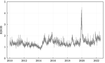
The main objective of this paper is to present an improved forecasting model for oil-based commodities. In this section, we demonstrate the importance of identifying the persistence structure on the volatility time series of oil-based commodities. Namely, we use the daily realised volatilities of three major energy commodities: crude oil (CL), natural gas (NG) and regular gasoline (RBOB). The data cover the period from January 2010 to December 2022, and realised volatilities are calculated from 5-minute returns. The left column of the figure (1) shows the time series of all three commodities.

Following Barunik and Vacha (2023), we use the multiscale impulse response functions from the TV-EWD model. Looking at the evolution of the volatility persistence structure gives us detailed information about the persistence of the shocks that generate the volatility time series of the energy commodities under study.

Figure 1: Left: Realized volatilities for crude oil (CL), natural gas (NG) and gasoline (RBOB). Right: Time-varying persistence structure of CL (top), NG (middle), RB (bottom). The plot shows the ratios of $\widehat{\beta}^{j}(t/T,1)/\sum_{j}\widehat{\beta}^{j}(t/T,1)$ on the y-axis, with $j$ corresponding to 2, 4, 8, 16, 32, 64, 128+ days persistence of the shocks represented by cold to warm colours, respectively, over the period from January 2010 to December 2022 on the x-axis.

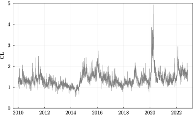
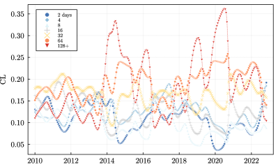
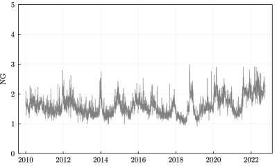
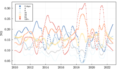
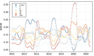
We begin by illustrating the persistence structure derived by our model. Figure (1) shows the evolution of the persistence structure of volatility. We report the persistence at a given scale $j$ as the persistence share of that scale relative to the persistence at other scales. More specifically, we compute the ratio of the first coefficient of the multiscale impulse response function $\widehat{\beta}^{j}(t/T,1)$ to the sum of the first coefficients of all scales $\sum_{j}\widehat{\beta}^{j}(t/T,1)$. The scales $j$ represent 2,4,8,16,32,64,128 days persistence of shocks and are represented in the figure from cold (scale 2) to warm (scale 128) colours (1). As the persistence structure is highly heterogeneous and time-varying, it motivates the use of the TV-EWD model for modelling and forecasting volatility. There are four notable sub-periods in which the persistence structure of volatility changes significantly:

• Before 2014: The volatility of CL is dominated by shocks of medium persistence (16-64 days), with transitory shocks (2-8 days) of rather low importance. In contrast, NG and RBOB volatilities are dominated by transitory shocks.

• Feb 2014 (annexation of Crimea): Significant increase in the longer-term volatility of oil and petrol, while petrol spikes only for very short periods. In December 2014, the oil price was 50% lower than in April 2014. Thus, oil volatility is mostly driven by persistent shocks of 64-128 days, which generate about 60% of the shocks in this period. Gas and petrol also show higher persistence.

• Onset of the Covid-19 pandemic: The beginning of 2020 is characterised by the oil price spike followed by a sharp drop, leading to very high volatility and persistence. Shocks with a persistence of 64 and 128+ days generate more than 50% of the volatility. Gasoline shows similar behaviour to oil. However, natural gas does not react as strongly to the pandemic, as we observe a mixture of transient and persistent shocks (almost homogeneous structure with equal persistence).

• Feb 2022: After the start of the aggression in February 2022, we observe the dominance of transitory shocks (2 and 4 day persistence accounts for 40%). For oil, transitory shocks also dominate in this period, but they are not as strong (2 and 4 day persistence accounts for 35%). This is a consequence of a very unstable and rapidly changing situation. After February 2022, we clearly observe an increase in overall volatility for all three commodities.

3.1 Volatility Forecasts

Having identified a rich dynamic in the volatility persistence of the three major energy commodities, we use it to build the forecasting model. The time-varying persistence structure shows that we often witness changes from the transient to the persistent nature of the shocks that dominate volatility. This motivates us to use the TV-EWD model, which can capture the non-trivial, possibly non-stationary dynamics of the volatility series.

To compare the forecasting performance of the TV-EWD model with other commonly used models for estimating the volatility of energy commodities, we use the models that best approximate persistence or long memory behaviour, such as the Heterogeneous Autoregressive Model (HAR) of Corsi (2009) and the EWD model of Ortu et al. (2020). This model also uses the extended Wold decomposition, but faces the same difficulties in capturing the time-varying nature of volatility time series. While both models capture the unconditional long-run dependence well, they assume stationarity of volatility. To assess the dynamic behaviour, we use both the simple TVP-AR(3) model and the TV-HAR model. The latter model is powerful in capturing the time-varying structure as well as in exploiting the heterogeneous horizon structure (persistence) as it allows for daily, weekly and monthly horizons. This makes the model very versatile and usually hard to beat as it is both highly effective and parsimonious.

Note that the kernel width is set to 0.3 and depth of decomposition is 7 scales which similar for all TV-EWD model settings. This means that the longest horizon considered is 128 and more days (128+). However, The TV-AR(p) model differs for prediction horizons as well as commodities. The TV-AR(p) model for CL has $p=2$ for the 1-day-ahead forecast and $p=6$ for the 5- and 22-day-ahead forecasts. For NG the TV-AR(p) model has $p=5$ for all forecasts, and for RB the TV-AR(p) model has $p=2$ for the 1-day-ahead forecast and $p=5$ for the 5- and 22-day-ahead forecasts.

Table 1: Root mean square error (RMSE) and mean absolute error (MAE) of the TV-EWD model compared to Ortu et al. (2020)’s extended wold decomposition (EWD), time-varying autoregression (TV-AR(3)). All errors are relative to the time-varying HAR (TV-HAR) model of Corsi (2009) over $h=1$, $h=5$ and $h=22$. Thus, the value bellow one implies that the corresponding model outperforms the TV-HAR benchmark. We use $*$,$**$ and $***$ to denote that a competing model has significantly lower MSE and MAE (is better) in comparison to the TV-HAR model at 90%, 95% and 99% significance levels, respectively. We use ${\dagger}$,${\dagger}{\dagger}$ and ${\dagger}{\dagger}{\dagger}$ to denote that a competing model has significantly higher MSE and MAE (is worse) in comparison to the TV-HAR model at 90%, 95% and 99% significance levels, respectively.

		RMSE				MAE
		$h=1$	$h=5$	$h=22$		$h=1$	$h=5$	$h=22$
	EWD	1.373†††	1.542†††	0.962		1.457†††	1.577†††	1.185†††
CL	TV-AR3	1.051††	1.062†	0.855∗∗∗		1.035†††	1.108†††	1.024
	TV-EWD	1.009	0.946∗	0.807∗∗∗		1.008	0.982	0.960∗∗
	EWD	1.297†††	1.381†††	1.235†††		1.437†††	1.621†††	1.358†††
NG	TV-AR3	1.064†††	1.134†††	1.300††		1.089†††	1.253†††	1.234†††
	TV-EWD	1.003	0.945∗∗	0.923∗∗∗		1.006	0.965∗∗∗	0.895∗∗∗
	EWD	1.249†††	1.444†††	1.125†††		1.481†††	1.535†††	1.299†††
RB	TV-AR3	1.052†††	1.112†††	0.997		1.084†††	1.186†††	1.105†††
	TV-EWD	1.000	0.954∗	0.880∗∗∗		1.017	1.003	0.951∗∗∗

Table 1 summarises the results of the volatility forecasting performance of the main energy commodities. We report the Root Mean Square Error (RMSE) and the Mean Absolute Error (MAE) loss functions. The TV-HAR model is used as a benchmark and all reported losses are relative to the TV-HAR. Thus, a value less (greater) than one indicates that the corresponding model has a better (worse) forecasting performance relative to the benchmark.

In general, the ability of the TV-EWD model to outperform all alternatives increases with increasing forecast horizons. TV-EWD provides significantly better forecasts than the benchmark in all cases for forecasts of 22 days ahead. The superior performance in the MAE also suggests that the forecasts are not systematically biased relative to the other models.

For the 5-day-ahead forecasts, the results are mixed. In terms of RMSE, the TV-EWD again outperforms the benchmark significantly. In terms of MAE, our model still provides significantly better forecasts for natural gas, but the forecasts for the other two commodities are indistinguishable from the TV-HAR. Similarly, the forecast errors of our approach and TV-HAR are the same for the 1-day-ahead forecast for both the RMSE and MAE loss functions.

The EWD model of Ortu et al. (2020) performs well for the 22-day-ahead forecasts as measured by the RMSE loss. This implies that the model is immune to large forecast outliers. Conversely, the poor performance, as measured by the MAE, indicates a systematic bias in the forecast. This is caused by a very slow adjustment to changes in the level of long-term volatility. This is a consequence of the model’s lack of time-varying capabilities.

4 Conclusion

In this paper, we study oil-based volatility and identify shocks with heterogeneous persistence that vary smoothly over time. Based on such dynamics, we construct a forecasting model that significantly outperforms alternative models, especially at longer horizons. The model provides valuable information about the fundamental behaviour of the volatility time series and is useful for both practitioners and policy makers.

As the paper introduces a novel decomposition of the volatility time series, it also opens up new avenues for further research. It would be interesting to learn about the dynamic persistence structure of other important energy data and, in particular, to use them in other forecasting or economic models.

References

- Arouri et al. (2012) Arouri, M. E. H., A. Lahiani, A. Lévy, and D. K. Nguyen (2012). Forecasting the conditional volatility of oil spot and futures prices with structural breaks and long memory models. Energy Economics 34(1), 283–293.
- Baillie et al. (1996) Baillie, R. T., C.-F. Chung, and M. A. Tieslau (1996). Analysing inflation by the fractionally integrated arfima–garch model. Journal of applied econometrics 11(1), 23–40.
- Bandi et al. (2021) Bandi, F. M., S. E. Chaudhuri, A. W. Lo, and A. Tamoni (2021). Spectral factor models. Journal of Financial Economics 142(1), 214–238.
- Bandi and Tamoni (2022) Bandi, F. M. and A. Tamoni (2022). Spectral financial econometrics. Econometric Theory 38(6), 1175–1220.
- Barunik and Vacha (2023) Barunik, J. and L. Vacha (2023). The dynamic persistence of economic shocks. Available at SSRN 4467110.
- Bollerslev and Engle (1993) Bollerslev, T. and R. F. Engle (1993). Common persistence in conditional variances. Econometrica: Journal of the Econometric Society 61(1), 167–186.
- Charfeddine (2014) Charfeddine, L. (2014). True or spurious long memory in volatility: Further evidence on the energy futures markets. Energy policy 71, 76–93.
- Corsi (2009) Corsi, F. (2009). A simple approximate long-memory model of realized volatility. Journal of Financial Econometrics 7(2), 174–196.
- Dahlhaus (1996) Dahlhaus, R. (1996). On the kullback-leibler information divergence of locally stationary processes. Stochastic processes and their applications 62(1), 139–168.
- Elder and Serletis (2010) Elder, J. and A. Serletis (2010). Oil price uncertainty. Journal of Money, Credit and Banking 42(6), 1137–1159.
- Fan and Gijbels (1996) Fan, J. and I. Gijbels (1996). Local polynomial modelling and its applications: monographs on statistics and applied probability 66, Volume 66. CRC Press.
- Granger and Ding (1996) Granger, C. W. and Z. Ding (1996). Varieties of long memory models. Journal of econometrics 73(1), 61–77.
- Granger and Hyung (2004) Granger, C. W. and N. Hyung (2004). Occasional structural breaks and long memory with an application to the s&p 500 absolute stock returns. Journal of empirical finance 11(3), 399–421.
- Hamilton (1983) Hamilton, J. D. (1983). Oil and the macroeconomy since world war ii. Journal of political economy 91(2), 228–248.
- Hamilton (2020) Hamilton, J. D. (2020). Time series analysis. Princeton university press.
- Haugom et al. (2014) Haugom, E., H. Langeland, P. Molnár, and S. Westgaard (2014). Forecasting volatility of the us oil market. Journal of Banking & Finance 47, 1–14.
- Herrera et al. (2018) Herrera, A. M., L. Hu, and D. Pastor (2018). Forecasting crude oil price volatility. International Journal of Forecasting 34(4), 622–635.
- Kang and Yoon (2013) Kang, S. H. and S.-M. Yoon (2013). Modeling and forecasting the volatility of petroleum futures prices. Energy Economics 36, 354–362.
- Kilian (2009) Kilian, L. (2009). Not all oil price shocks are alike: Disentangling demand and supply shocks in the crude oil market. American Economic Review 99(3), 1053–1069.
- Le et al. (2023) Le, T.-H., S. Boubaker, M. T. Bui, and D. Park (2023). On the volatility of wti crude oil prices: A time-varying approach with stochastic volatility. Energy Economics 117, 106474.
- Lu et al. (2022) Lu, F., F. Ma, P. Li, and D. Huang (2022). Natural gas volatility predictability in a data-rich world. International Review of Financial Analysis 83, 102218.
- Ma et al. (2017) Ma, F., M. I. M. Wahab, D. Huang, and W. Xu (2017). Forecasting the realized volatility of the oil futures market: A regime switching approach. Energy Economics 67, 136–145.
- Ortu et al. (2020) Ortu, F., F. Severino, A. Tamoni, and C. Tebaldi (2020). A persistence-based wold-type decomposition for stationary time series. Quantitative Economics 11(1), 203–230.
- Ozdemir et al. (2013) Ozdemir, Z. A., K. Gokmenoglu, and C. Ekinci (2013). Persistence in crude oil spot and futures prices. Energy 59, 29–37.
- Sévi (2014) Sévi, B. (2014). Forecasting the volatility of crude oil futures using intraday data. European Journal of Operational Research 235(3), 643–659.
- Stărică and Granger (2005) Stărică, C. and C. Granger (2005). Nonstationarities in stock returns. Review of economics and statistics 87(3), 503–522.
- Wang and Wu (2012) Wang, Y. and C. Wu (2012). Long memory in energy futures markets: Further evidence. Resources Policy 37(3), 261–272.
- Wang et al. (2016) Wang, Y., C. Wu, and L. Yang (2016). Forecasting crude oil market volatility: A markov switching multifractal volatility approach. International Journal of Forecasting 32(1), 1–9.
- Wen et al. (2016) Wen, F., X. Gong, and S. Cai (2016). Forecasting the volatility of crude oil futures using har-type models with structural breaks. Energy Economics 59, 400–413.
- Wold (1938) Wold, H. (1938). A study in the analysis of stationary time series. Almquist & Wiksells Boktryckeri.
- Zhang et al. (2019) Zhang, Y., Y. Wei, Y. Zhang, and D. Jin (2019). Forecasting oil price volatility: Forecast combination versus shrinkage method. Energy Economics 80, 423–433.