On the power of linear programming for K-means clustering

Abstract

In [5], the authors introduced a new linear programming (LP) relaxation for K-means clustering. In this paper, we further investigate the theoretical properties of this relaxation. We focus on K-means clustering with two clusters, which is an NP-hard problem. As evident from our numerical experiments with both synthetic and real-world data sets, the proposed LP relaxation is almost always tight; i.e., its optimal solution is feasible for the original nonconvex problem. To better understand this unexpected behaviour, we obtain sufficient conditions under which the LP relaxation is tight. We further analyze the sufficient conditions when the input is generated according to a popular stochastic model and obtain recovery guarantees for the LP relaxation. Finally, we construct a family of inputs for which the LP relaxation is never tight.

Key words. K-means clustering; Linear programming relaxation; Ratio-cut polytope; Tightness; Recovery guarantee.

1 Introduction

Clustering data points into a small number of groups according to some similarity measure is a common task in unsupervised machine learning, and is ubiquitous across operations research and engineering. K-means clustering, one of the oldest and the most popular clustering techniques, partitions the data points into clusters by minimizing the total squared distance between each data point and the corresponding cluster center. Let $\{x^{i}\}_{i=1}^{n}$ denote a set of $n$ data points in ${\mathbb{R}}^{m}$, and denote by $K$ the number of desired clusters. Define a partition of $[n]:=\{1,\ldots,n\}$ as a family $\{\Gamma_{k}\}_{k=1}^{K}$ of non-empty subsets of $[n]$ such that $\Gamma_{a}\cap\Gamma_{b}=\emptyset$ for all $a\neq b\in[K]$ and $\cup_{k\in[K]}{\Gamma_{k}}=[n]$. Then K-means clustering can be formulated as a combinatorial optimization problem:

$$\min\quad \sum_{k=1}^{K}{\sum_{i\in\Gamma_{k}}{\Big{\lVert}x^{i}-\frac{1}{|\Gamma_{k}|}\sum_{j\in\Gamma_{k}}{x^{j}}\Big{\rVert}_{2}^{2}}}$$ (1)

s.t. $$\{\Gamma_{k}\}_{k\in[K]}\;{\rm is\;a\;partition\;of\;[n]}.$$

It is well-known that Problem (1) is NP-hard even when there are only two clusters [2] or when the data points are in ${\mathbb{R}}^{2}$ [13]. The most popular techniques for solving Problem (1) are heuristics such as Lloyd’s algorithm [12], approximation algorithms [10, 7], and convex relaxations [17, 16, 3, 15, 9, 11, 5]. The two prominent types of convex relaxations for K-means clustering are semi-definite programming (SDP) relaxations [16] and linear programming (LP) relaxations [5]. The theoretical properties of SDP relaxations for K-means clustering have been thoroughly studied in the literature [3, 15, 9, 19, 11]. In this paper we investigate the power of LP relaxations for K-means clustering. To this end, in the following, we present an alternative formulation for Problem (1), which we use to construct our relaxations.

Consider a partition $\{\Gamma_{k}\}_{k=1}^{K}$ of $[n]$; let ${\bf 1}_{\Gamma_{k}}$, $k\in[K]$ be the indicator vector of the $k$th cluster; i.e., the $i$th component of ${\bf 1}_{\Gamma_{k}}$ is defined as: $({\bf 1}_{\Gamma_{k}})_{i}=1$ if $i\in\Gamma_{k}$ and $({\bf 1}_{\Gamma_{k}})_{i}=0$ otherwise. Define the associated partition matrix as:

$$X=\sum_{k=1}^{K}{\frac{1}{|\Gamma_{k}|}{\bf 1}_{\Gamma_{k}}{\bf 1}^{T}_{\Gamma_{k}}}.$$ (2)

Define $d_{ij}:=||x^{i}-x^{j}||_{2}^{2}$ for all $i,j\in[n]$. Then Problem (1) can be equivalently written as (see [11] for detailed derivation):

$$\min\quad \sum_{i,j\in[n]}{d_{ij}X_{ij}}$$ (3)

s.t. $$X\;{\rm is\;a\;partition\;matrix\;defined\;by~{}\eqref{pm}}.$$

It can be checked that any partition matrix $X$ is positive semidefinite. Using this observation, one can obtain the following SDP relaxation of Problem (3):

$$\min\quad \sum_{i,j\in[n]}{d_{ij}X_{ij}}$$ (PW)

s.t. $${\rm Tr}(X)=K,$$

$$\sum_{j=1}^{n}X_{ij}=1,\quad\forall i\in[n],$$

$$X\succeq 0,$$

$$X_{ij}\geq 0,\quad X_{ij}=X_{ji},\quad\forall 1\leq i<j\leq n,$$

where ${\rm Tr}(X)$ is the trace of the matrix $X$, and $X\succeq 0$ means that $X$ is positive semidefinite. The above relaxation was first proposed in [16] and is often referred to as the “Peng-Wei SDP relaxation”. Both theoretical and numerical properties of this relaxation have been thoroughly investigated in the literature [3, 15, 9, 11, 18].

1.1 LP relaxations for K-means clustering

In [5], the authors introduced the ratio-cut polytope, defined as the convex hull of ratio-cut vectors corresponding to all partitions of $n$ points in ${\mathbb{R}}^{m}$ into at most $K$ clusters. They showed this polytope is closely related to the convex hull of the feasible region of Problem (3). The authors then studied the facial structure of the ratio-cut polytope, which in turn enabled them to obtain a new family of LP relaxations for K-means clustering. Fix a parameter $t\in\{2,\ldots,K\}$; then an LP relaxation for K-means clustering is given by:

$$\min\quad \sum_{i,j\in[n]}{d_{ij}X_{ij}}$$

s.t. $$\text{Tr}(X)=K,$$

$$\sum_{j=1}^{n}X_{ij}=1,\quad\forall i\in[n],$$

$$\sum_{j\in S}{X_{ij}}\leq X_{ii}+\sum_{j,k\in S:j<k}{X_{jk}},\quad\forall i\in[n],\;\forall S\subseteq[n]\setminus\{i\}:2\leq|S|\leq t,$$ (4)

$$X_{ij}\geq 0,\quad X_{ij}=X_{ji},\quad\forall 1\leq i<j\leq n.$$

We should remark that by Proposition 3 of [5], inequalities (4) define facets of the convex hull of the feasible region of Problem (3). It then follows that for any $t<t^{\prime}$, the feasible region of Problem (LPK${}_{t^{\prime}}$) is strictly contained in the feasible region of Problem (LPK_t). In [3], the authors propose and study a different LP relaxation for K-means clustering. As it is detailed in [5], for any $t\geq 2$, the feasible region of Problem (1.1) is strictly contained in that of the LP relaxation considered in [3] (see Remark 1 in [5]). In fact, the numerical experiments on synthetic data in [5] indicate that Problem (1.1) with $t=2$ is almost always tight; i.e., the optimal solution of the LP is a partition matrix. To better understand this unexpected behaviour, in this paper, we perform a theoretical study of the tightness of the (1.1) relaxation. As a first step, we consider the case of two clusters. Performing a similar type of analysis for $K>2$ is a topic of future research.

Our main contributions are summarized as follows:

• Consider any partition of $[n]$ and the associated partition matrix $X$ defined by (2). By constructing a dual certificate, we obtain a sufficient condition, often referred to as a “proximity condition”, under which $X$ is the unique optimal solution of Problem (1.1) (see Proposition 1 and Proposition 3). This result can be considered as a generalization of Theorem 1 in [5] where the optimality of equal-size clusters is studied. Our proximity condition is overly conservative since, to obtain an explicit condition, we fix a subset of the dual variables to zero. To address this, we propose a simple algorithm to carefully assign values to dual variables previously set to zero, leading to a significantly better dual certificate for $X$ (see Proposition 5).

• Consider a generative model, referred to as the stochastic sphere model (SSM), in which there are two clusters of possibly different size in ${\mathbb{R}}^{m}$, and the data points in each cluster are sampled from a uniform distribution on a sphere of unit radius. Using the result of part (i) we obtain a sufficient condition in terms of the distance between sphere centers under which the (1.1) relaxation recovers the planted clusters with high probability. By high probability we mean the probability tending to one as the number of data points tends to infinity (see Proposition 4).

• Since in almost all our experiments with synthetic and real-world data sets Problem (1.1) is tight, it is natural to ask whether the (1.1) relaxation is tight with high probability under reasonable generative models. We present a family of inputs for which the (1.1) relaxation is never tight (see Proposition 6 and Corollary 1).

1.2 Organization

The rest of the paper is structured as follows. In Section 2, we motivate our study by demonstrating that for both synthetic and real-world data sets, the LP relaxation defined by Problem (1.1) is almost always tight. In Section 3, we present a sufficient condition under which a given partition matrix is the unique optimal solution of the (1.1) relaxation for two clusters. Using this sufficient condition, in Section 4 we obtain a recovery guarantee for the (1.1) relaxation under the SSM. In Section 5, we present a simple algorithm to construct a stronger dual certificate for an optimal partition matrix. Finally, in Section 6 we present a family of inputs for which the optimal value of the (1.1) relaxation is strictly smaller than the optimal value of the K-means clustering problem.

2 The LP relaxation for two clusters

In this paper, we study the case with two clusters and examine the strength of the LP relaxation theoretically. Recall that for $K=2$, Problem (1.1) requires $t=2$ and it simplifies to:

$$\min\quad \sum_{i,j\in[n]}{d_{ij}X_{ij}}$$

s.t. $$\text{Tr}(X)=2,$$ (5)

$$\sum_{j=1}^{n}X_{ij}=1,\quad\forall 1\leq i\leq n,$$ (6)

$$X_{ij}+X_{ik}\leq X_{ii}+X_{jk},\quad\forall i\neq j\neq k\in[n],\;j<k,$$ (7)

$$X_{ij}\geq 0,\quad\forall 1\leq i<j\leq n,$$ (8)

where as before we set $X_{ji}=X_{ij}$ for all $1\leq i<j\leq n$. Henceforth, whenever we say “the LP relaxation,” we mean the LP defined by Problem (2) and whenever we say “the SDP relaxation,” we mean the SDP defined by Problem (PW). To motivate our theoretical study, in the following we conduct some numerical experiments to convey the power of the LP relaxation for clustering both synthetic and real-world data sets.

2.1 Numerical experiments

In the following, we compare the strength of the LP relaxation defined by Problem (2) with the SDP relaxation defined by Problem (PW). It is important to note that solving both LP and SDP become computationally expensive as we increase the number of points $n$. That is, to solve an instance with $n\gtrsim 200$ efficiently, one needs to design a specialized algorithm for both LP (such as cutting plane algorithms) and SDP (such as first-order methods). Indeed, in [18] the authors design a specialized algorithm for the SDP relaxation and solve problems with $n\leq 4000$. Designing a customized algorithm to solve the LP relaxation is a topic of our future research. In this paper, however, we are interested in performing a theoretical analysis of the tightness of the LP and we are using our numerical experiments to motivate this study. Hence, in this paper, we limit ourselves to solving problem instances with $n\leq 200$ variables.

In the following, we consider both synthetic and real-world data sets. We say that a convex relaxation is tight if its optimal solution is a partition matrix. In [17] the authors prove that a symmetric matrix $X$ with unit row-sums and trace $K$ is a partition matrix if and only if it is a projection matrix; i.e., $X^{T}X=X$. Hence to check whether the solution of the LP relaxation or the SDP relaxation is tight, we check whether it is a projection matrix. All experiments are performed on the NEOS server [4]; LPs are solved with GAMS/Gurobi [8] and SDPs are solved with GAMS/MOSEK [1]. We deactivated the crossover operation in all Gurobi runs. All other options are set to their default values for both solvers.

2.1.1 Synthetic data

One of the most popular generative models for K-means clustering is the stochastic ball model (SBM). In this model, we assume that the data in each cluster is sampled from a uniform distribution within a ball of unit radius and the difficulty of the problem is measured by the distance $\Delta$ between the balls’ centers. In our experiments, we set the number of clusters $K=2$, the number of points $n=100$, and the input dimension $m=10$. We denote the number of points sampled from the first (resp. the second) ball by $n_{1}$ (resp. by $n_{2}$). We consider two configurations: (i) $n_{1}=n_{2}$ and (ii) $n_{1}=0.3n_{2}$. For each fixed configuration $(n_{1},n_{2})$, we consider various values for $\Delta$; namely, we set $\Delta\in[0:0.01:2]$. For each fixed $\Delta$, we conduct 20 random trials. We count the number of times the optimization algorithm returns a partition matrix as the optimal solution; dividing this number by the total number of trials, we obtain the empirical tightness rate.

Our results are shown in Figure 1: the LP relaxation significantly outperforms the SDP relaxation. That is, out of a total of $4000$ runs, the LP relaxation is not tight only in $9$ cases; i.e., an overall tightness rate of $0.9975$. In contrast, the SDP is tight only when the data in the two clusters are sufficiently separated, with an overall tightness rate of $0.4755$. Moreover, in all cases for which the SDP is not tight, its optimal objective value is strictly smaller than that of the LP. To further illustrate this point, we have also plotted the average percentage of the relative gap between the SDP optimal value $f_{\rm SDP}$ and the LP optimal value $f_{\rm LP}$, defined as $g_{\rm rel}=\frac{f_{\rm LP}-f_{\rm SDP}}{f_{\rm LP}}\times 100$.

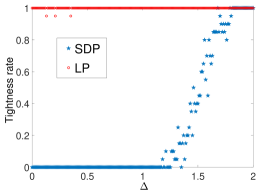
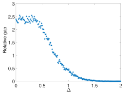
(a) $n_{1}=n_{2}$

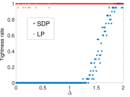
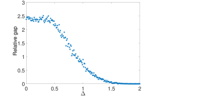
(b) $n_{1}=0.3n_{2}$

Figure 1: Comparing the strength of the LP relaxation versus the SDP relaxation for K-means clustering when the input is generated according to the SBM in ${\mathbb{R}}^{10}$ with $n=n_{1}+n_{2}=100$ points, where $n_{1}$ is the number of points sampled from the first ball and $n_{2}$ is the number of points sampled from the second ball.

2.1.2 Real-world data

We collected a set of 15 data sets from the UCI machine learning repository [6]. These problems come from diverse applications and have been extensively used as benchmarks to compare the performance of different clustering algorithms in the literature. The data sets and their characteristics, i.e., the number of points $n$ and the input dimension $m$ are listed in columns 1-3 of Table 1. For data sets with $n\leq 200$ (i.e., Voice, Iris, and Wine), we solve the clustering problem over the entire data set. For each of the remaining data sets, to control the computational cost of both LP and SDP, we sample ten times $n^{\prime}=200$ data points and solve LP and SDP using the ten random instances. The tightness rate of the LP ($t_{\rm LP}$), the tightness rate of the SDP ($t_{\rm SDP}$), and the (average) relative gap between the optimal values of SDP and LP are listed in columns 4-6 of Table 1. In all instances, the LP relaxation is tight, while the SDP is only tight in a few instances.

The remarkable performance of the LP relaxation is indeed unexpected and hence in this paper, it is our goal to better understand this behaviour through a theoretical study.

Table 1: Comparing the strength of the LP relaxation versus the SDP relaxation for clustering real-world data sets: $t_{\rm LP}$ denotes the tightness rate of the LP, $t_{\rm SDP}$ denotes the tightness rate of the SDP, $g_{\rm rel}$ denotes the (average) percentage of relative gap between the optimal values of SDP and LP.

Data set	$n$	$m$	$t_{\rm LP}$	$t_{\rm SDP}$	$g_{\rm rel}$ (%)
Voice	126	310	1.0	0.0	5.40
Iris	150	4	1.0	0.0	1.09
Wine	178	13	1.0	0.0	3.44
Seeds	210	7	1.0	0.0	3.80
Accent	329	12	1.0	0.3	0.02
ECG5000	500	140	1.0	0.1	0.07
Hungarian	522	20	1.0	0.0	1.01
Wdbc	569	30	1.0	0.0	5.51
Strawberry	613	235	1.0	0.0	5.40
Energy	768	16	1.0	1.0	0.0
SalesWeekly	810	106	1.0	0.0	1.74
Vehicle	846	18	1.0	0.0	1.11
Wafer	1000	152	1.0	0.3	0.06
Ethanol	2000	27	1.0	1.0	0.0
Rice	3810	7	1.0	0.0	1.70

3 A sufficient condition for tightness of the LP relaxation

We first obtain a sufficient “proximity” condition under which Problem (2) is tight; i.e., the optimal solution of the LP relaxation is a partition matrix. A proximity condition for the SDP relaxation defined by Problem (PW) is presented in [11]. As our proximity condition is overly conservative, we then present a simple algorithm that certifies the optimality of a given partition matrix.

To establish our proximity condition, in Proposition 1, we first obtain a sufficient condition under which a given partition matrix is an optimal solution of Problem (2). Subsequently in Proposition 3, we address the question of uniqueness of the optimal solution. The next proposition can be considered as a generalization of Theorem 1 in [5] where the authors study the optimality of equal-size clusters.

In the following, for every $A\subseteq[n]$ and $f:A\to{\mathbb{R}}$, we define

$$\underset{i\in A}{\mathchoice{{\vbox{\hbox{$\textstyle-$ }}\kern-9.7222pt}}{{\vbox{\hbox{$\scriptstyle-$ }}\kern-8.11111pt}}{{\vbox{\hbox{$\scriptscriptstyle-$ }}\kern-6.19444pt}}{{\vbox{\hbox{$\scriptscriptstyle-$ }}\kern-5.13889pt}}\!\sum}{f(i)}:=\frac{1}{|A|}\sum_{i\in A}{f(i)}.$$

Moreover, given a partition $\{\Gamma_{1},\Gamma_{2}\}$ of $[n]$, for each $i\in\Gamma_{l}$, $l\in\{1,2\}$, we define

$$d^{\text{in}}_{i}:=\underset{j\in\Gamma_{l}}{\mathchoice{{\vbox{\hbox{$\textstyle-$ }}\kern-9.7222pt}}{{\vbox{\hbox{$\scriptstyle-$ }}\kern-8.11111pt}}{{\vbox{\hbox{$\scriptscriptstyle-$ }}\kern-6.19444pt}}{{\vbox{\hbox{$\scriptscriptstyle-$ }}\kern-5.13889pt}}\!\sum}{d_{ij}},$$

and

$$d^{\text{out}}_{i}:=\underset{j\in[n]\setminus\Gamma_{l}}{\mathchoice{{\vbox{\hbox{$\textstyle-$ }}\kern-9.7222pt}}{{\vbox{\hbox{$\scriptstyle-$ }}\kern-8.11111pt}}{{\vbox{\hbox{$\scriptscriptstyle-$ }}\kern-6.19444pt}}{{\vbox{\hbox{$\scriptscriptstyle-$ }}\kern-5.13889pt}}\!\sum}{d_{ij}}.$$

We are now ready to state our sufficient condition.

Proposition 1.

Let $\{\Gamma_{1},\Gamma_{2}\}$ denote a partition of $[n]$ and assume without loss of generality that $|\Gamma_{1}|\leq|\Gamma_{2}|$. Define

$$r_{1}:=\frac{2|\Gamma_{1}|}{|\Gamma_{1}|+|\Gamma_{2}|},\quad r_{2}:=\frac{2|\Gamma_{2}|}{|\Gamma_{1}|+|\Gamma_{2}|},$$ (9)

and

$$\eta:=\frac{r_{2}}{2}\Bigg{(}\Big{(}1-\frac{r_{1}}{r_{2}}\Big{)}\max_{k\in\Gamma_{1}}d^{\text{in}}_{k}+\Big{(}1-\frac{r_{2}}{r_{1}}\Big{)}\min_{k\in\Gamma_{2}}d^{\text{in}}_{k}+\frac{r_{1}}{r_{2}}\underset{k\in\Gamma_{1}}{\mathchoice{{\vbox{\hbox{$\textstyle-$ }}\kern-9.7222pt}}{{\vbox{\hbox{$\scriptstyle-$ }}\kern-8.11111pt}}{{\vbox{\hbox{$\scriptscriptstyle-$ }}\kern-6.19444pt}}{{\vbox{\hbox{$\scriptscriptstyle-$ }}\kern-5.13889pt}}\!\sum}{d^{\text{in}}_{k}}+\frac{r_{2}}{r_{1}}\underset{k\in\Gamma_{2}}{\mathchoice{{\vbox{\hbox{$\textstyle-$ }}\kern-9.7222pt}}{{\vbox{\hbox{$\scriptstyle-$ }}\kern-8.11111pt}}{{\vbox{\hbox{$\scriptscriptstyle-$ }}\kern-6.19444pt}}{{\vbox{\hbox{$\scriptscriptstyle-$ }}\kern-5.13889pt}}\!\sum}{d^{\text{in}}_{k}}\Bigg{)}.$$ (10)

Suppose that

$$\underset{k\in\Gamma_{2}}{\mathchoice{{\vbox{\hbox{$\textstyle-$ }}\kern-9.7222pt}}{{\vbox{\hbox{$\scriptstyle-$ }}\kern-8.11111pt}}{{\vbox{\hbox{$\scriptscriptstyle-$ }}\kern-6.19444pt}}{{\vbox{\hbox{$\scriptscriptstyle-$ }}\kern-5.13889pt}}\!\sum}{\min\{r_{2}d_{ik}+d^{\text{in}}_{j},r_{2}d_{jk}+d^{\text{in}}_{i}\}}-d_{ij}\geq\eta,\quad\forall i<j\in\Gamma_{1},$$ (11)

and

$$\underset{k\in\Gamma_{1}}{\mathchoice{{\vbox{\hbox{$\textstyle-$ }}\kern-9.7222pt}}{{\vbox{\hbox{$\scriptstyle-$ }}\kern-8.11111pt}}{{\vbox{\hbox{$\scriptscriptstyle-$ }}\kern-6.19444pt}}{{\vbox{\hbox{$\scriptscriptstyle-$ }}\kern-5.13889pt}}\!\sum}{\min\{r_{1}d_{ik}+d^{\text{in}}_{j},r_{1}d_{jk}+d^{\text{in}}_{i}\}}-d_{ij}\geq\frac{r_{1}}{r_{2}}\eta,\quad\forall i<j\in\Gamma_{2}.$$ (12)

Then, an optimal solution of Problem (2) is given by the partition matrix

$$\bar{X}=\frac{1}{|\Gamma_{1}|}{\bf 1}_{\Gamma_{1}}{\bf 1}^{T}_{\Gamma_{1}}+\frac{1}{|\Gamma_{2}|}{\bf 1}_{\Gamma_{2}}{\bf 1}^{T}_{\Gamma_{2}}.$$ (13)

Proof.

We start by constructing the dual of Problem (2). Define dual variables $\omega$ associated with (5), $\mu_{i}$ for all $i\in[n]$ associated with (6), $\lambda_{ijk}$ for all $(i,j,k)\in\Omega:=\{(i,j,k):i\neq j\neq k\in[n],\;j<k\}$ associated with (7), and $\sigma_{ij}$ for all $1\leq i<j\leq n$ associated with (8). The dual of Problem (2) is then given by:

$$\max\quad -(2\omega+\sum_{i\in[n]}{\mu_{i}})$$

s.t. $$\mu_{i}+\mu_{j}+\sum_{k\in[n]\setminus\{i,j\}}{(\lambda_{ijk}+\lambda_{jik}-\lambda_{kij})}+2d_{ij}-\sigma_{ij}=0,\;\forall 1\leq i<j\leq n,$$ (14)

$$\omega+\mu_{i}-\sum_{j,k\in[n]\setminus\{i\}:j<k}{\lambda_{ijk}}=0,\;\forall i\in[n],$$ (15)

$$\lambda_{ijk}\geq 0,\quad\forall(i,j,k)\in\Omega,\quad\sigma_{ij}\geq 0,\quad\forall 1\leq i<j\leq n,$$

where we let $\lambda_{ikj}=\lambda_{ijk}$ for all $(i,j,k)\in\Omega$. To establish the optimality of $\bar{X}$ defined by (13), it suffices to construct a dual feasible point $(\bar{\lambda},\bar{\mu},\bar{\omega},\bar{\sigma})$ that together with $\bar{X}$ satisfies the complementary slackness. Without loss of generality, assume that $i<j$ for all $i\in\Gamma_{1}$ and $j\in\Gamma_{2}$. Then $\bar{X}$ and $(\bar{\lambda},\bar{\mu},\bar{\omega},\bar{\sigma})$ satisfy the complementary slackness if and only if:

• $\bar{\lambda}_{ijk}=0$ if $i\in\Gamma_{1}$ and $j,k\in\Gamma_{2}$ or if $i\in\Gamma_{2}$ and $j,k\in\Gamma_{1}$,

• $\bar{\sigma}_{ij}=0$ if $i,j\in\Gamma_{1}$ or $i,j\in\Gamma_{2}$.

After projecting out $\bar{\sigma}_{ij}$ for $i\in\Gamma_{1}$ and $j\in\Gamma_{2}$, we deduce that it suffices to find $(\bar{\lambda},\bar{\mu},\bar{\omega})$ satisfying:

$$\bar{\mu}_{i}+\bar{\mu}_{j}+\sum_{k\notin\Gamma_{l}}{(\bar{\lambda}_{ijk}+\bar{\lambda}_{jik})}+\sum_{k\in\Gamma_{l}\setminus\{i,j\}}{(\bar{\lambda}_{ijk}+\bar{\lambda}_{jik}-\bar{\lambda}_{kij})}+2d_{ij}=0,\quad\forall i<j\in\Gamma_{l},l\in\{1,2\}$$ (16)

$$\bar{\mu}_{i}+\bar{\mu}_{j}+\sum_{k\in\Gamma_{1}\setminus\{i\}}{(\bar{\lambda}_{ijk}-\bar{\lambda}_{kij})}+\sum_{k\in\Gamma_{2}\setminus\{j\}}{(\bar{\lambda}_{jik}-\bar{\lambda}_{kij})}+2d_{ij}\geq 0,\quad\forall i\in\Gamma_{1},j\in\Gamma_{2}$$ (17)

$$\bar{\omega}+\bar{\mu}_{i}-\sum_{\begin{subarray}{c}j\in\Gamma_{l}\setminus\{i\},\\ k\notin\Gamma_{l}\end{subarray}}{\bar{\lambda}_{ijk}}-\sum_{j<k\in\Gamma_{l}\setminus\{i\}}{\bar{\lambda}_{ijk}}=0,\quad\forall i\in\Gamma_{l},l\in\{1,2\}.$$ (18)

To this end, let

$$\bar{\lambda}_{ijk}-\bar{\lambda}_{jik}=\frac{d_{jk}-d_{ik}}{n/2}+\frac{d^{\text{in}}_{i}-d^{\text{in}}_{j}}{|\Gamma_{2}|},\quad\forall i,j\in\Gamma_{1},k\in\Gamma_{2}$$ (19)

$$\bar{\lambda}_{ijk}-\bar{\lambda}_{jik}=\frac{d_{jk}-d_{ik}}{n/2}+\frac{d^{\text{in}}_{i}-d^{\text{in}}_{j}}{|\Gamma_{1}|},\quad\forall i,j\in\Gamma_{2},k\in\Gamma_{1}$$ (20)

$$\bar{\mu}_{i}=-d^{\text{in}}_{i}-r_{2}d^{\text{out}}_{i}+\eta,\quad\forall i\in\Gamma_{1}$$ (21)

$$\bar{\mu}_{i}=-d^{\text{in}}_{i}-r_{1}d^{\text{out}}_{i}+\frac{r_{1}}{r_{2}}\eta,\quad\forall i\in\Gamma_{2}$$ (22)

$$\bar{\omega}=-\frac{1}{2}\sum_{i\in[n]}{(d^{\text{in}}_{i}+\bar{\mu}_{i})},$$ (23)

where $r_{1},r_{2}$ and $\eta$ are as defined by (9) and (10), respectively.

First let us examine the validity of inequalities (17). Substituting (19)-(22) in (17) yields:

$$-d^{\text{in}}_{i}-r_{2}d^{\text{out}}_{i}+\eta-d^{\text{in}}_{j}-r_{1}d^{\text{out}}_{j}+\frac{r_{1}}{r_{2}}\eta+\sum_{k\in\Gamma_{1}\setminus\{i\}}{\Big{(}\frac{d_{jk}-d_{ij}}{n/2}+\frac{d^{\text{in}}_{i}-d^{\text{in}}_{k}}{|\Gamma_{2}|}\Big{)}}$$

$$+\sum_{k\in\Gamma_{2}\setminus\{j\}}{\Big{(}\frac{d_{ik}-d_{ij}}{n/2}+\frac{d^{\text{in}}_{j}-d^{\text{in}}_{k}}{|\Gamma_{1}|}\Big{)}}+2d_{ij}=$$

$$-d^{\text{in}}_{i}-r_{2}d^{\text{out}}_{i}+\eta-d^{\text{in}}_{j}-r_{1}d^{\text{out}}_{j}+\frac{r_{1}}{r_{2}}\eta+r_{1}d^{\text{out}}_{j}-r_{1}d_{ij}+\frac{r_{1}}{r_{2}}d^{\text{in}}_{i}-\frac{r_{1}}{r_{2}}\underset{k\in\Gamma_{1}}{\mathchoice{{\vbox{\hbox{$\textstyle-$ }}\kern-9.7222pt}}{{\vbox{\hbox{$\scriptstyle-$ }}\kern-8.11111pt}}{{\vbox{\hbox{$\scriptscriptstyle-$ }}\kern-6.19444pt}}{{\vbox{\hbox{$\scriptscriptstyle-$ }}\kern-5.13889pt}}\!\sum}{d^{\text{in}}_{k}}+r_{2}d^{\text{out}}_{i}-r_{2}d_{ij}+$$

$$\frac{r_{2}}{r_{1}}d^{\text{in}}_{j}-\frac{r_{2}}{r_{1}}\underset{k\in\Gamma_{2}}{\mathchoice{{\vbox{\hbox{$\textstyle-$ }}\kern-9.7222pt}}{{\vbox{\hbox{$\scriptstyle-$ }}\kern-8.11111pt}}{{\vbox{\hbox{$\scriptscriptstyle-$ }}\kern-6.19444pt}}{{\vbox{\hbox{$\scriptscriptstyle-$ }}\kern-5.13889pt}}\!\sum}{d^{\text{in}}_{k}}+2d_{ij}=$$

$$\Big{(}1+\frac{r_{1}}{r_{2}}\Big{)}\eta-\Big{(}1-\frac{r_{1}}{r_{2}}\Big{)}d^{\text{in}}_{i}-\Big{(}1-\frac{r_{2}}{r_{1}}\Big{)}d^{\text{in}}_{j}-\frac{r_{1}}{r_{2}}\underset{k\in\Gamma_{1}}{\mathchoice{{\vbox{\hbox{$\textstyle-$ }}\kern-9.7222pt}}{{\vbox{\hbox{$\scriptstyle-$ }}\kern-8.11111pt}}{{\vbox{\hbox{$\scriptscriptstyle-$ }}\kern-6.19444pt}}{{\vbox{\hbox{$\scriptscriptstyle-$ }}\kern-5.13889pt}}\!\sum}{d^{\text{in}}_{k}}-\frac{r_{2}}{r_{1}}\underset{k\in\Gamma_{2}}{\mathchoice{{\vbox{\hbox{$\textstyle-$ }}\kern-9.7222pt}}{{\vbox{\hbox{$\scriptstyle-$ }}\kern-8.11111pt}}{{\vbox{\hbox{$\scriptscriptstyle-$ }}\kern-6.19444pt}}{{\vbox{\hbox{$\scriptscriptstyle-$ }}\kern-5.13889pt}}\!\sum}{d^{\text{in}}_{k}}\geq 0,$$

where the last inequality follows from the definition of $\eta$ given by (10) and the identity $r_{1}+r_{2}=2$.

We now show that equalities (18) are implied by equalities (16). In the following we prove that all equalities of the form (18) with $l=1$ are implied by equalities of the form (16) with $l=1$; the proof of the case with $l=2$ follows from a similar line of arguments. Using (19) to eliminate $\bar{\lambda}_{jik}$ for $i,j\in\Gamma_{1}$ and $k\in\Gamma_{2}$, and using (21) to eliminate $\bar{\mu}_{i}$, $i\in\Gamma_{1}$, it follows that equalities (16) with $l=1$ can be equivalently written as:

$$\sum_{k\in\Gamma_{2}}{\bar{\lambda}_{ijk}}+\frac{1}{2}\sum_{k\in\Gamma_{1}\setminus\{i,j\}}{(\bar{\lambda}_{ijk}+\bar{\lambda}_{jik}-\bar{\lambda}_{kij})}=d^{\text{in}}_{i}+r_{2}d^{\text{out}}_{j}-d_{ij}-\eta,\quad\forall i<j\in\Gamma_{1}.$$ (24)

Using (21)-(23), inequalities (18) can be written as:

$$\sum_{\begin{subarray}{c}j\in\Gamma_{1}\setminus\{i\},\\ k\in\Gamma_{2}\end{subarray}}{\bar{\lambda}_{ijk}}+\sum_{j<k\in\Gamma_{1}\setminus\{i\}}{\bar{\lambda}_{ijk}}=r_{2}\sum_{j\in\Gamma_{1}}{d^{\text{out}}_{j}}-d^{\text{in}}_{i}-r_{2}d^{\text{out}}_{i}-(|\Gamma_{1}|-1)\eta,\quad\forall i\in\Gamma_{1},$$ (25)

where we used the identity $r_{2}\sum_{j\in\Gamma_{1}}{d^{\text{out}}_{i}}=r_{1}\sum_{j\in\Gamma_{2}}{d^{\text{out}}_{i}}$. Moreover, it can be checked that

$$\sum_{j\neq k\in\Gamma_{1}\setminus\{i\}}{(\bar{\lambda}_{ijk}+\bar{\lambda}_{jik}-\bar{\lambda}_{kij})}=2\sum_{j<k\in\Gamma_{1}\setminus\{i\}}{\bar{\lambda}_{ijk}}.$$

Therefore, to show that equalities (25) are implied by equalities (24), it suffices to have:

$$\sum_{j\in\Gamma_{1}\setminus\{i\}}{(d^{\text{in}}_{i}+r_{2}d^{\text{out}}_{j}-d_{ij}-\eta)}=r_{2}\sum_{j\in\Gamma_{1}}{d^{\text{out}}_{j}}-d^{\text{in}}_{i}-r_{2}d^{\text{out}}_{i}-(|\Gamma_{1}|-1)\eta,$$

whose validity follows since $\sum_{j\in\Gamma_{1}\setminus\{i\}}{(d^{\text{in}}_{i}-d_{ij})}=(|\Gamma_{1}|-1)d^{\text{in}}_{i}-|\Gamma_{1}|d^{\text{in}}_{i}=d^{\text{in}}_{i}$.

Therefore, it remains to prove the validity of equalities (16). First consider the case with $l=1$. By (19) and nonnegativity of $\bar{\lambda}_{ijk}$ for all $(i,j,k)\in\Omega$, we deduce that

$$\bar{\lambda}_{ijk}+\bar{\lambda}_{jik}\geq{\rm abs}\left(\frac{d_{jk}-d_{ik}}{n/2}+\frac{d^{\text{in}}_{i}-d^{\text{in}}_{j}}{|\Gamma_{2}|}\right)=\frac{1}{|\Gamma_{2}|}{\rm abs}\Big{(}(d^{\text{in}}_{i}+r_{2}d_{jk})-(d^{\text{in}}_{j}+r_{2}d_{ik})\Big{)},\quad\forall i,j\in\Gamma_{1},k\in\Gamma_{2},$$

where ${\rm abs}(\cdot)$ denote the absolute value function. Hence, using (21) to eliminate $\bar{\mu}_{i}$, we conclude that equalities (16) with $l=1$ can be satisfied if

$$\frac{1}{2}\sum_{k\in\Gamma_{1}\setminus\{i,j\}}{(\bar{\lambda}_{ijk}+\bar{\lambda}_{jik}-\bar{\lambda}_{kij})}\leq\underset{k\in\Gamma_{2}}{\mathchoice{{\vbox{\hbox{$\textstyle-$ }}\kern-9.7222pt}}{{\vbox{\hbox{$\scriptstyle-$ }}\kern-8.11111pt}}{{\vbox{\hbox{$\scriptscriptstyle-$ }}\kern-6.19444pt}}{{\vbox{\hbox{$\scriptscriptstyle-$ }}\kern-5.13889pt}}\!\sum}{\min\{r_{2}d_{ik}+d^{\text{in}}_{j},r_{2}d_{jk}+d^{\text{in}}_{i}\}}-d_{ij}-\eta,\quad\forall i<j\in\Gamma_{1},$$ (26)

where we used the identity ${\rm abs}(a-b)=a+b-2\min\{a,b\}$. Letting $\bar{\lambda}_{ijk}=0$ for all $(i,j,k)\in\Gamma_{1}$ and using (11), we conclude that inequalities (26) are valid. Similarly, it can be checked that inequalities (17) with $l=2$ can be satisfied if

$$\frac{1}{2}\sum_{k\in\Gamma_{2}\setminus\{i,j\}}{(\bar{\lambda}_{ijk}+\bar{\lambda}_{jik}-\bar{\lambda}_{kij})}\leq\underset{k\in\Gamma_{1}}{\mathchoice{{\vbox{\hbox{$\textstyle-$ }}\kern-9.7222pt}}{{\vbox{\hbox{$\scriptstyle-$ }}\kern-8.11111pt}}{{\vbox{\hbox{$\scriptscriptstyle-$ }}\kern-6.19444pt}}{{\vbox{\hbox{$\scriptscriptstyle-$ }}\kern-5.13889pt}}\!\sum}{\min\{r_{1}d_{ik}+d^{\text{in}}_{j},r_{1}d_{jk}+d^{\text{in}}_{i}\}}-d_{ij}-\frac{r_{1}}{r_{2}}\eta,\quad\forall i<j\in\Gamma_{2}.$$ (27)

Letting $\bar{\lambda}_{ijk}=0$ for all $(i,j,k)\in\Gamma_{2}$ and using (12), we conclude that inequalities (27) are valid and this completes the proof. ∎

We now consider the question of uniqueness of the optimal solution. To this end, we make use of the following result:

Proposition 2 (Part (iv) of Theorem 2 in [14]).

Consider an LP whose feasible region is defined by $Ax=b$ and $Cx\leq d$, where $x\in{\mathbb{R}}^{n}$ denotes the vector of optimization variables, and $b,d,A,C$ are vectors and matrices of appropriate dimensions. Let $\bar{x}$ be an optimal solution of this LP and denote by $\bar{u}$ the dual optimal solution corresponding to the inequality constraints. Let $C_{i}$ denote the $i$-th row of $C$. Define $Q=\{i:C_{i}\bar{x}=d_{i},\;\bar{u}_{i}>0\}$, $L=\{i:C_{i}\bar{x}=d_{i},\;\bar{u}_{i}=0\}$. Let $\mathscr{C}_{Q}$ and $\mathscr{C}_{L}$ be the matrices whose rows are $C_{i}$, $i\in Q$ and $C_{i}$, $i\in L$, respectively. Then $\bar{x}$ is the unique optimal solution of the LP, if there exists no $x$ different from the zero vector satisfying

$$Ax=0,\quad\mathscr{C}_{Q}x=0,\quad\mathscr{C}_{L}x\leq 0.$$ (28)

We are now ready to establish our uniqueness result:

Proposition 3.

Suppose that inequalities (11) and (12) are strictly satisfied. Then $\bar{X}$ defined by (13) is the unique optimal solution of Problem (2).

Proof.

Consider the dual certificate $(\bar{\lambda},\bar{\mu},\bar{\omega},\bar{\sigma})$ constructed in the proof of Proposition 1. We consider a slightly modified version of this certificate by redefining $\eta$ defined in (10) as follows:

$$\eta=\frac{r_{2}}{2}\Bigg{(}\Big{(}1-\frac{r_{1}}{r_{2}}\Big{)}\max_{k\in\Gamma_{1}}d^{\text{in}}_{k}+\Big{(}1-\frac{r_{2}}{r_{1}}\Big{)}\min_{k\in\Gamma_{2}}d^{\text{in}}_{k}+\frac{r_{1}}{r_{2}}\underset{k\in\Gamma_{1}}{\mathchoice{{\vbox{\hbox{$\textstyle-$ }}\kern-9.7222pt}}{{\vbox{\hbox{$\scriptstyle-$ }}\kern-8.11111pt}}{{\vbox{\hbox{$\scriptscriptstyle-$ }}\kern-6.19444pt}}{{\vbox{\hbox{$\scriptscriptstyle-$ }}\kern-5.13889pt}}\!\sum}{d^{\text{in}}_{k}}+\frac{r_{2}}{r_{1}}\underset{k\in\Gamma_{2}}{\mathchoice{{\vbox{\hbox{$\textstyle-$ }}\kern-9.7222pt}}{{\vbox{\hbox{$\scriptstyle-$ }}\kern-8.11111pt}}{{\vbox{\hbox{$\scriptscriptstyle-$ }}\kern-6.19444pt}}{{\vbox{\hbox{$\scriptscriptstyle-$ }}\kern-5.13889pt}}\!\sum}{d^{\text{in}}_{k}}\Bigg{)}+\epsilon,$$

for some $\epsilon>0$. This in turn will imply that $\bar{\sigma}_{ij}>0$ for all $i\in\Gamma_{1}$, $j\in\Gamma_{2}$. Notice that this is an admissible modification as we are assuming that inequalities (11) and (12) are strictly satisfied. In addition, we can choose

$$\bar{\lambda}_{ijk}>\max\Big{\{}0,\frac{d_{jk}-d_{ik}}{n/2}+\frac{d^{\text{in}}_{i}-d^{\text{in}}_{j}}{|\Gamma_{2}|}\Big{\}},\;\bar{\lambda}_{jik}>\max\Big{\{}0,\frac{d_{ik}-d_{jk}}{n/2}+\frac{d^{\text{in}}_{j}-d^{\text{in}}_{i}}{|\Gamma_{2}|}\Big{\}},\;\forall i,j\in\Gamma_{1},k\in\Gamma_{2}$$

$$\bar{\lambda}_{ijk}>\max\Big{\{}0,\frac{d_{jk}-d_{ik}}{n/2}+\frac{d^{\text{in}}_{i}-d^{\text{in}}_{j}}{|\Gamma_{1}|}\Big{\}},\;\bar{\lambda}_{jik}>\max\Big{\{}0,\frac{d_{ik}-d_{jk}}{n/2}+\frac{d^{\text{in}}_{j}-d^{\text{in}}_{i}}{|\Gamma_{1}|}\Big{\}},\;\forall i,j\in\Gamma_{2},k\in\Gamma_{1}.$$

Therefore, by Proposition 2, the matrix $\bar{X}$ defined by (13) is the unique optimal solution of Problem (2), if there exists no $X\neq 0$ satisfying:

$$\sum_{j=1}^{n}{X_{ij}}=0,\quad\forall 1\leq i\leq n$$ (29)

$$X_{ij}=0,\quad\forall i\in\Gamma_{1},j\in\Gamma_{2}$$ (30)

$$X_{ij}+X_{ik}=X_{ii}+X_{jk},\quad\forall i,j\in\Gamma_{1},k\in\Gamma_{2},\;{\rm or}\;i,j\in\Gamma_{2},k\in\Gamma_{1}.$$ (31)

From (29) and (30) it follows that

$$X_{ii}+\sum_{j\in\Gamma_{1}}{X_{ij}}=0,\quad\forall i\in\Gamma_{1},\quad X_{ii}+\sum_{j\in\Gamma_{2}}{X_{ij}}=0,\quad\forall i\in\Gamma_{2}.$$ (32)

Moreover, from equations (31) we deduce that

$$X_{ij}=\frac{X_{ii}+X_{jj}}{2},\quad\forall i,j\in\Gamma_{1}\;{\rm or}\;i,j\in\Gamma_{2}.$$ (33)

Substituting (33) in (32) we obtain:

$$X_{ii}=X_{ij}=0,\quad\forall i,j\in\Gamma_{1},\;{\rm or}\;i,j\in\Gamma_{2},$$

which together with (30) completes the proof. ∎

Using our proximity condition given by inequalities (11) and (12), we next obtain a recovery guarantee for the LP relaxation under a popular stochastic model for the input data.

4 Recovery guarantee for the stochastic sphere model

It is widely understood that worst-case guarantees for optimization algorithms are often too pessimistic. A recent line of research in data clustering is concerned with obtaining sufficient conditions under which a planted clustering corresponds to the unique optimal solution of a convex relaxation under suitable stochastic models [3, 15, 9, 11, 5]. Such conditions are often referred to as (exact) recovery conditions and are used to compare the strength of various convex relaxations for NP-hard problems. Henceforth, we say that an optimization problem recovers the planted clusters if its unique optimal solution corresponds to the planted clusters.

Perhaps the most popular generative model for K-means clustering is the stochastic ball model, where the points are sampled from uniform distributions on $K$ unit balls in ${\mathbb{R}}^{m}$. As before, we let $K=2$ and we denote by $\Delta$ the distance between the ball centers. Notice that the question of recovery only makes sense when $\Delta>2$, whereas the question of tightness is well-defined for any $\Delta\geq 0$. We denote by $\Gamma_{1}$ and $\Gamma_{2}$ the set of points sampled from the first and second balls, respectively and without loss of generality we assume $|\Gamma_{1}|\leq|\Gamma_{2}|$. In the following, whenever we say with high probability, we mean the probability tending to one as $n\rightarrow\infty$. In [11], the authors prove that the Peng-Wei SDP relaxation defined by Problem (PW) recovers the planted clusters with high probability if

$$\Delta>2\Big{(}1+\sqrt{\frac{1}{r_{1}(m+2)}}\Big{)},$$ (34)

where $r_{1}$ is defined by (9). In the special case of equal-size clusters, i.e., $|\Gamma_{1}|=|\Gamma_{2}|$, the authors of [3] show that the Peng-Wei SDP relaxation recovers the planted clusters with high probability, if $\Delta>2\sqrt{2}(1+\frac{1}{\sqrt{m}})$, while the authors of [9] show that the same SDP recovers the planted clusters with high probability if $\Delta>2(1+\frac{2}{m})$. Again, for equal-size clusters, in [5], the authors show that Problem (2) recovers the planted clusters with high probability, if $\Delta>1+\sqrt{3}$.

In this section, we obtain a recovery guarantee for the LP relaxation for two clusters of arbitrary size. For simplicity, we consider a slightly different stochastic model, which we refer to as the stochastic sphere model (SSM), where instead of a ball, the points in each clusters are sampled from a sphere (i.e., the boundary of a ball). We prove that our deterministic optimality condition given by inequalities (11)-(12) implies that Problem (2) recovers the planted clusters with high probability, if

$$\Delta>1+\sqrt{1+\frac{2}{r_{1}}}.$$ (35)

We should mention that, at the expense of a significantly longer proof, one can obtain the same recovery guarantee (35) for the LP relaxation under the SBM. We do not include the latter result in this paper because, while the proof is more technical and longer, it does not contain any new ideas and closely follows the path of our proof for the SSM. Indeed, in the case of equal-size clusters; i.e., $r_{1}=1$, inequality (35) simplifies to the recovery guarantee of [5] for SBM: $\Delta>1+\sqrt{3}$. Also note that while the recovery guarantee for the LP (35) is better than the the recovery guarantee for the SDP (34) for $1\leq m\leq 5$, it becomes weaker for larger dimensions. As we detail in the next section, condition (35) can be significantly improved via a more careful selection of the dual certificate.

Throughout this section, for an event $A$, we denote by $\operatorname{\mathbb{P}}(A)$ the probability of $A$. For a random variable $Y$, we denote by $\operatorname{\mathbb{E}}[Y]$ its expected value. In case of a multivariate random variable $X_{ij}$, the conditional expected value in $j$, with $i$ fixed, will be denoted either with $\operatorname{\mathbb{E}}_{i}[X]$ or with $\operatorname{\mathbb{E}}^{j}[X]$. We denote by $\partial{\mathcal{B}}_{1}$ and $\partial{\mathcal{B}}_{2}$ the spheres corresponding to the first and second clusters, respectively. Up to a rotation we can assume that the centers of $\partial{\mathcal{B}}_{1}$ and $\partial{\mathcal{B}}_{2}$ are $0$ and $\Delta e_{1}$, respectively, where $e_{1}$ is the first vector of the standard basis of ${\mathbb{R}}^{m}$. For a continuous function $f:\partial{\mathcal{B}}_{1}\to{\mathbb{R}}$ (and analogously for $\partial{\mathcal{B}}_{2}$), we define

$$\mathchoice{{\vbox{\hbox{$\textstyle-$ }}\kern-7.83337pt}}{{\vbox{\hbox{$\scriptstyle-$ }}\kern-5.90005pt}}{{\vbox{\hbox{$\scriptscriptstyle-$ }}\kern-4.75003pt}}{{\vbox{\hbox{$\scriptscriptstyle-$ }}\kern-4.25003pt}}\!\int_{\partial{\mathcal{B}}_{1}}f(x)d{\mathcal{H}}^{m-1}(x):=\frac{1}{{\mathcal{H}}^{m-1}(\partial{\mathcal{B}}_{1})}\int_{\partial{\mathcal{B}}_{1}}f(x)d{\mathcal{H}}^{m-1}(x),$$

where ${\mathcal{H}}^{m-1}(x)$ denotes the $(m-1)$-dimensional Hausdorff measure.

We are now ready to state our recovery result.

Proposition 4.

Suppose that the points are generated according to the SSM. Then Problem (2) recovers the planted clusters with high probability if $\Delta>\Delta_{0}:=1+\sqrt{1+\frac{2}{r_{1}}}$, where $r_{1}$ is defined by (9).

Proof.

By Proposition 3, it suffices to show that for $\Delta>\Delta_{0}$, inequalities (11)-(12) are strictly satisfied with high probability. Namely, we show that there exists a universal constant $C>0$ such that, for $\Delta>\Delta_{0}$ we have

$$\begin{split}\operatorname{\mathbb{P}}\Big{(}\bigcap_{i,j\in\Gamma_{1}}\Big{\{}d_{ij}+\eta-\underset{k\in\Gamma_{2}}{\mathchoice{{\vbox{\hbox{$\textstyle-$ }}\kern-9.7222pt}}{{\vbox{\hbox{$\scriptstyle-$ }}\kern-8.11111pt}}{{\vbox{\hbox{$\scriptscriptstyle-$ }}\kern-6.19444pt}}{{\vbox{\hbox{$\scriptscriptstyle-$ }}\kern-5.13889pt}}\!\sum}{\min\{r_{2}d_{ik}+d^{\text{in}}_{j},r_{2}d_{jk}+d^{\text{in}}_{i}\}}<0\Big{\}}\Big{)}\geq 1-Cn^{2}e^{-\frac{n\epsilon^{2}_{2}}{C}}\end{split}$$ (36)

and

$$\begin{split}\operatorname{\mathbb{P}}\Big{(}\bigcap_{i,j\in\Gamma_{2}}\Big{\{}d_{ij}+\frac{r_{1}}{r_{2}}\eta-\underset{k\in\Gamma_{1}}{\mathchoice{{\vbox{\hbox{$\textstyle-$ }}\kern-9.7222pt}}{{\vbox{\hbox{$\scriptstyle-$ }}\kern-8.11111pt}}{{\vbox{\hbox{$\scriptscriptstyle-$ }}\kern-6.19444pt}}{{\vbox{\hbox{$\scriptscriptstyle-$ }}\kern-5.13889pt}}\!\sum}{\min\{r_{1}d_{ik}+d^{\text{in}}_{j},r_{1}d_{jk}+d^{\text{in}}_{i}\}}<0\Big{\}}\Big{)}\geq 1-Cn^{2}e^{-\frac{n\epsilon^{2}_{1}}{C}},\end{split}$$

where $\epsilon_{1},\epsilon_{2}>0$ are as defined in the statement of Lemma 1. Since the two inequalities are symmetric, their proof is similar and we will only prove inequality (36).

To this aim, for notational simplicity, define

$$t_{ij}:=\operatorname{\mathbb{E}}^{k}\Big{[}\underset{k\in\Gamma_{2}}{\mathchoice{{\vbox{\hbox{$\textstyle-$ }}\kern-9.7222pt}}{{\vbox{\hbox{$\scriptstyle-$ }}\kern-8.11111pt}}{{\vbox{\hbox{$\scriptscriptstyle-$ }}\kern-6.19444pt}}{{\vbox{\hbox{$\scriptscriptstyle-$ }}\kern-5.13889pt}}\!\sum}{\min\{r_{2}d_{ik}+\operatorname{\mathbb{E}}_{j}[d^{\text{in}}_{j}],r_{2}d_{jk}+\operatorname{\mathbb{E}}_{i}[d^{\text{in}}_{i}]\}}\Big{]}.$$

Then we can compute

$$\begin{split}&\operatorname{\mathbb{P}}\Big{(}\bigcap_{i,j\in\Gamma_{1}}\Big{\{}d_{ij}+\eta-\underset{k\in\Gamma_{2}}{\mathchoice{{\vbox{\hbox{$\textstyle-$ }}\kern-9.7222pt}}{{\vbox{\hbox{$\scriptstyle-$ }}\kern-8.11111pt}}{{\vbox{\hbox{$\scriptscriptstyle-$ }}\kern-6.19444pt}}{{\vbox{\hbox{$\scriptscriptstyle-$ }}\kern-5.13889pt}}\!\sum}{\min\{r_{2}d_{ik}+d^{\text{in}}_{j},r_{2}d_{jk}+d^{\text{in}}_{i}\}}<0\Big{\}}\Big{)}\\ &\geq\operatorname{\mathbb{P}}\Big{(}\bigcap_{i,j\in\Gamma_{1}}\Big{\{}d_{ij}+\eta-d_{ij}-2r_{2}+t_{ij}-\underset{k\in\Gamma_{2}}{\mathchoice{{\vbox{\hbox{$\textstyle-$ }}\kern-9.7222pt}}{{\vbox{\hbox{$\scriptstyle-$ }}\kern-8.11111pt}}{{\vbox{\hbox{$\scriptscriptstyle-$ }}\kern-6.19444pt}}{{\vbox{\hbox{$\scriptscriptstyle-$ }}\kern-5.13889pt}}\!\sum}{\min\{r_{2}d_{ik}+d^{\text{in}}_{j},r_{2}d_{jk}+d^{\text{in}}_{i}\}}<4\epsilon_{2}\Big{\}}\Big{)}\\ &\geq\operatorname{\mathbb{P}}\Big{(}\Big{\{}\Big{|}\eta-2r_{2}\Big{|}<2\epsilon_{2}\Big{\}}\cap\bigcap_{i,j\in\Gamma_{1}}\Big{\{}\Big{|}t_{ij}-\operatorname{\mathbb{E}}^{k}\Big{[}\underset{k\in\Gamma_{2}}{\mathchoice{{\vbox{\hbox{$\textstyle-$ }}\kern-9.7222pt}}{{\vbox{\hbox{$\scriptstyle-$ }}\kern-8.11111pt}}{{\vbox{\hbox{$\scriptscriptstyle-$ }}\kern-6.19444pt}}{{\vbox{\hbox{$\scriptscriptstyle-$ }}\kern-5.13889pt}}\!\sum}{\min\{r_{2}d_{ik}+d^{\text{in}}_{j},r_{2}d_{jk}+d^{\text{in}}_{i}\}}\Big{]}\Big{|}<\epsilon_{2}\Big{\}}\\ &\cap\bigcap_{i,j\in\Gamma_{1}}\Big{\{}\Big{|}\operatorname{\mathbb{E}}^{k}\Big{[}\underset{k\in\Gamma_{2}}{\mathchoice{{\vbox{\hbox{$\textstyle-$ }}\kern-9.7222pt}}{{\vbox{\hbox{$\scriptstyle-$ }}\kern-8.11111pt}}{{\vbox{\hbox{$\scriptscriptstyle-$ }}\kern-6.19444pt}}{{\vbox{\hbox{$\scriptscriptstyle-$ }}\kern-5.13889pt}}\!\sum}{\min\{r_{2}d_{ik}+d^{\text{in}}_{j},r_{2}d_{jk}+d^{\text{in}}_{i}\}}\Big{]}-\underset{k\in\Gamma_{2}}{\mathchoice{{\vbox{\hbox{$\textstyle-$ }}\kern-9.7222pt}}{{\vbox{\hbox{$\scriptstyle-$ }}\kern-8.11111pt}}{{\vbox{\hbox{$\scriptscriptstyle-$ }}\kern-6.19444pt}}{{\vbox{\hbox{$\scriptscriptstyle-$ }}\kern-5.13889pt}}\!\sum}{\min\{r_{2}d_{ik}+d^{\text{in}}_{j},r_{2}d_{jk}+d^{\text{in}}_{i}\}}\Big{|}<\epsilon_{2}\Big{\}}\Big{)}\\ &\geq 1-\operatorname{\mathbb{P}}(\{|\eta-2r_{2}|\geq 2\epsilon_{2}\})-\operatorname{\mathbb{P}}\Big{(}\bigcup_{i,j\in\Gamma_{1}}\Big{\{}\Big{|}t_{ij}-\operatorname{\mathbb{E}}^{k}\Big{[}\underset{k\in\Gamma_{2}}{\mathchoice{{\vbox{\hbox{$\textstyle-$ }}\kern-9.7222pt}}{{\vbox{\hbox{$\scriptstyle-$ }}\kern-8.11111pt}}{{\vbox{\hbox{$\scriptscriptstyle-$ }}\kern-6.19444pt}}{{\vbox{\hbox{$\scriptscriptstyle-$ }}\kern-5.13889pt}}\!\sum}{\min\{r_{2}d_{ik}+d^{\text{in}}_{j},r_{2}d_{jk}+d^{\text{in}}_{i}\}}\Big{]}\Big{|}\geq\epsilon_{2}\Big{\}}\Big{)}\\ &-\operatorname{\mathbb{P}}\Big{(}\bigcup_{i,j\in\Gamma_{1}}\Big{\{}\Big{|}\operatorname{\mathbb{E}}^{k}\Big{[}\underset{k\in\Gamma_{2}}{\mathchoice{{\vbox{\hbox{$\textstyle-$ }}\kern-9.7222pt}}{{\vbox{\hbox{$\scriptstyle-$ }}\kern-8.11111pt}}{{\vbox{\hbox{$\scriptscriptstyle-$ }}\kern-6.19444pt}}{{\vbox{\hbox{$\scriptscriptstyle-$ }}\kern-5.13889pt}}\!\sum}{\min\{r_{2}d_{ik}+d^{\text{in}}_{j},r_{2}d_{jk}+d^{\text{in}}_{i}\}}\Big{]}-\underset{k\in\Gamma_{2}}{\mathchoice{{\vbox{\hbox{$\textstyle-$ }}\kern-9.7222pt}}{{\vbox{\hbox{$\scriptstyle-$ }}\kern-8.11111pt}}{{\vbox{\hbox{$\scriptscriptstyle-$ }}\kern-6.19444pt}}{{\vbox{\hbox{$\scriptscriptstyle-$ }}\kern-5.13889pt}}\!\sum}{\min\{r_{2}d_{ik}+d^{\text{in}}_{j},r_{2}d_{jk}+d^{\text{in}}_{i}\}}\Big{|}\geq\epsilon_{2}\Big{\}}\Big{)}\end{split}$$ (37)

The first inequality follows from (47) in Lemma 1, since $\Delta>\Delta_{0}$; the second inequality holds by set inclusion, and the third inequality is obtained by taking the union bound. To complete the proof, we next estimate each of the terms in the last two lines of (37). In the following, $C$ will always denote a universal positive constant, which may increase from one line to the next line and we will not relabel it for the sake of exposition.

First, to estimate $\operatorname{\mathbb{P}}(\{|\eta-2r_{2}|\geq 2\epsilon_{2}\})$, we define

$$\eta_{1}:=\frac{r_{2}}{2}\Bigg{(}\Big{(}1-\frac{r_{1}}{r_{2}}\Big{)}\max_{k\in\Gamma_{1}}d^{\text{in}}_{k}+\Big{(}1-\frac{r_{2}}{r_{1}}\Big{)}\min_{k\in\Gamma_{2}}d^{\text{in}}_{k}\Bigg{)},\quad\eta_{2}:=\frac{r_{2}}{2}\Bigg{(}\frac{r_{1}}{r_{2}}\underset{k\in\Gamma_{1}}{\mathchoice{{\vbox{\hbox{$\textstyle-$ }}\kern-9.7222pt}}{{\vbox{\hbox{$\scriptstyle-$ }}\kern-8.11111pt}}{{\vbox{\hbox{$\scriptscriptstyle-$ }}\kern-6.19444pt}}{{\vbox{\hbox{$\scriptscriptstyle-$ }}\kern-5.13889pt}}\!\sum}{d^{\text{in}}_{k}}+\frac{r_{2}}{r_{1}}\underset{k\in\Gamma_{2}}{\mathchoice{{\vbox{\hbox{$\textstyle-$ }}\kern-9.7222pt}}{{\vbox{\hbox{$\scriptstyle-$ }}\kern-8.11111pt}}{{\vbox{\hbox{$\scriptscriptstyle-$ }}\kern-6.19444pt}}{{\vbox{\hbox{$\scriptscriptstyle-$ }}\kern-5.13889pt}}\!\sum}{d^{\text{in}}_{k}}\Bigg{)},$$ (38)

so that $\eta=\eta_{1}+\eta_{2}$. Recall that $|\Gamma_{1}|=r_{1}\frac{n}{2}$, $|\Gamma_{2}|=r_{2}\frac{n}{2}$, $r_{1}\in(0,1]$ and $r_{2}\in[1,2)$. Since for $\Delta>4$, the recovery follows from a simple thresholding argument, we can restrict our attention to $\Delta\leq 4$, i.e., we assume that $r_{1}\geq\frac{1}{4}$. It then follows that

$$\begin{split}\operatorname{\mathbb{P}}&(\{|\eta_{2}-\operatorname{\mathbb{E}}[\eta_{2}]|\geq\epsilon_{2}\})\\ &=\operatorname{\mathbb{P}}\Big{(}\Big{|}r_{1}\Bigg{(}\underset{i,j\in\Gamma_{1}}{\mathchoice{{\vbox{\hbox{$\textstyle-$ }}\kern-9.7222pt}}{{\vbox{\hbox{$\scriptstyle-$ }}\kern-8.11111pt}}{{\vbox{\hbox{$\scriptscriptstyle-$ }}\kern-6.19444pt}}{{\vbox{\hbox{$\scriptscriptstyle-$ }}\kern-5.13889pt}}\!\sum}d_{ij}-\operatorname{\mathbb{E}}\Big{[}\underset{i,j\in\Gamma_{1}}{\mathchoice{{\vbox{\hbox{$\textstyle-$ }}\kern-9.7222pt}}{{\vbox{\hbox{$\scriptstyle-$ }}\kern-8.11111pt}}{{\vbox{\hbox{$\scriptscriptstyle-$ }}\kern-6.19444pt}}{{\vbox{\hbox{$\scriptscriptstyle-$ }}\kern-5.13889pt}}\!\sum}d_{ij}\Big{]}\Bigg{)}+\frac{r_{2}^{2}}{r_{1}}\Bigg{(}\operatorname{\mathbb{E}}\Big{[}\underset{i,j\in\Gamma_{2}}{\mathchoice{{\vbox{\hbox{$\textstyle-$ }}\kern-9.7222pt}}{{\vbox{\hbox{$\scriptstyle-$ }}\kern-8.11111pt}}{{\vbox{\hbox{$\scriptscriptstyle-$ }}\kern-6.19444pt}}{{\vbox{\hbox{$\scriptscriptstyle-$ }}\kern-5.13889pt}}\!\sum}d_{ij}\Big{]}-\underset{i,j\in\Gamma_{2}}{\mathchoice{{\vbox{\hbox{$\textstyle-$ }}\kern-9.7222pt}}{{\vbox{\hbox{$\scriptstyle-$ }}\kern-8.11111pt}}{{\vbox{\hbox{$\scriptscriptstyle-$ }}\kern-6.19444pt}}{{\vbox{\hbox{$\scriptscriptstyle-$ }}\kern-5.13889pt}}\!\sum}d_{ij}\Bigg{)}\Big{|}\geq 2\epsilon_{2}\Big{)}\\ &\leq\operatorname{\mathbb{P}}\Big{(}\Big{\{}\Big{|}\underset{i,j\in\Gamma_{1}}{\mathchoice{{\vbox{\hbox{$\textstyle-$ }}\kern-9.7222pt}}{{\vbox{\hbox{$\scriptstyle-$ }}\kern-8.11111pt}}{{\vbox{\hbox{$\scriptscriptstyle-$ }}\kern-6.19444pt}}{{\vbox{\hbox{$\scriptscriptstyle-$ }}\kern-5.13889pt}}\!\sum}d_{ij}-\operatorname{\mathbb{E}}\Big{[}\underset{i,j\in\Gamma_{1}}{\mathchoice{{\vbox{\hbox{$\textstyle-$ }}\kern-9.7222pt}}{{\vbox{\hbox{$\scriptstyle-$ }}\kern-8.11111pt}}{{\vbox{\hbox{$\scriptscriptstyle-$ }}\kern-6.19444pt}}{{\vbox{\hbox{$\scriptscriptstyle-$ }}\kern-5.13889pt}}\!\sum}d_{ij}\Big{]}\Big{|}\geq\frac{\epsilon_{2}}{C}\Big{\}}\cup\Big{\{}\Big{|}\operatorname{\mathbb{E}}\Big{[}\underset{i,j\in\Gamma_{2}}{\mathchoice{{\vbox{\hbox{$\textstyle-$ }}\kern-9.7222pt}}{{\vbox{\hbox{$\scriptstyle-$ }}\kern-8.11111pt}}{{\vbox{\hbox{$\scriptscriptstyle-$ }}\kern-6.19444pt}}{{\vbox{\hbox{$\scriptscriptstyle-$ }}\kern-5.13889pt}}\!\sum}d_{ij}\Big{]}-\underset{i,j\in\Gamma_{2}}{\mathchoice{{\vbox{\hbox{$\textstyle-$ }}\kern-9.7222pt}}{{\vbox{\hbox{$\scriptstyle-$ }}\kern-8.11111pt}}{{\vbox{\hbox{$\scriptscriptstyle-$ }}\kern-6.19444pt}}{{\vbox{\hbox{$\scriptscriptstyle-$ }}\kern-5.13889pt}}\!\sum}d_{ij}\Big{|}\geq\frac{\epsilon_{2}}{C}\Big{\}}\Big{)}\\ &\leq\operatorname{\mathbb{P}}\Big{(}\Big{|}\underset{i,j\in\Gamma_{1}}{\mathchoice{{\vbox{\hbox{$\textstyle-$ }}\kern-9.7222pt}}{{\vbox{\hbox{$\scriptstyle-$ }}\kern-8.11111pt}}{{\vbox{\hbox{$\scriptscriptstyle-$ }}\kern-6.19444pt}}{{\vbox{\hbox{$\scriptscriptstyle-$ }}\kern-5.13889pt}}\!\sum}d_{ij}-\operatorname{\mathbb{E}}\Big{[}\underset{i,j\in\Gamma_{1}}{\mathchoice{{\vbox{\hbox{$\textstyle-$ }}\kern-9.7222pt}}{{\vbox{\hbox{$\scriptstyle-$ }}\kern-8.11111pt}}{{\vbox{\hbox{$\scriptscriptstyle-$ }}\kern-6.19444pt}}{{\vbox{\hbox{$\scriptscriptstyle-$ }}\kern-5.13889pt}}\!\sum}d_{ij}\Big{]}\Big{|}\geq\frac{\epsilon_{2}}{C}\Big{)}+\operatorname{\mathbb{P}}\Big{(}\Big{|}\operatorname{\mathbb{E}}\Big{[}\underset{i,j\in\Gamma_{2}}{\mathchoice{{\vbox{\hbox{$\textstyle-$ }}\kern-9.7222pt}}{{\vbox{\hbox{$\scriptstyle-$ }}\kern-8.11111pt}}{{\vbox{\hbox{$\scriptscriptstyle-$ }}\kern-6.19444pt}}{{\vbox{\hbox{$\scriptscriptstyle-$ }}\kern-5.13889pt}}\!\sum}d_{ij}\Big{]}-\underset{i,j\in\Gamma_{2}}{\mathchoice{{\vbox{\hbox{$\textstyle-$ }}\kern-9.7222pt}}{{\vbox{\hbox{$\scriptstyle-$ }}\kern-8.11111pt}}{{\vbox{\hbox{$\scriptscriptstyle-$ }}\kern-6.19444pt}}{{\vbox{\hbox{$\scriptscriptstyle-$ }}\kern-5.13889pt}}\!\sum}d_{ij}\Big{|}\geq\frac{\epsilon_{2}}{C}\Big{)}\leq Ce^{-\frac{n^{2}\epsilon_{2}^{2}}{C}}.\end{split}$$ (39)

The first inequality holds by set inclusion and the third inequality follows from Hoeffding’s inequality (see for example Theorem 2.2.6 in [20]), since $d_{ij}$, $i,j\in\Gamma_{l}$ are i.i.d. random variables for every $l\in\{1,2\}$ and $d_{ij}\in[0,4]$. Next we show that

$$\operatorname{\mathbb{P}}\Big{(}\Big{\{}\Big{|}\eta_{1}-\Big{(}2r_{2}-r_{1}-\frac{r_{2}^{2}}{r_{1}}\Big{)}\Big{|}\geq\epsilon_{2}\Big{\}}\Big{)}\leq Cne^{-\frac{n\epsilon_{2}^{2}}{C}}.$$ (40)

For notational simplicity, we denote the $i$th point in $\Gamma_{1}$ by $x$. We notice that for any $i\in\Gamma_{1}$ we have

$$\begin{split}\operatorname{\mathbb{E}}_{i}[d^{\text{in}}_{i}]&=\mathchoice{{\vbox{\hbox{$\textstyle-$ }}\kern-7.83337pt}}{{\vbox{\hbox{$\scriptstyle-$ }}\kern-5.90005pt}}{{\vbox{\hbox{$\scriptscriptstyle-$ }}\kern-4.75003pt}}{{\vbox{\hbox{$\scriptscriptstyle-$ }}\kern-4.25003pt}}\!\int_{\partial{\mathcal{B}}_{1}}\|x-z\|^{2}d{\mathcal{H}}^{m-1}(z)=\|x\|^{2}+\mathchoice{{\vbox{\hbox{$\textstyle-$ }}\kern-7.83337pt}}{{\vbox{\hbox{$\scriptstyle-$ }}\kern-5.90005pt}}{{\vbox{\hbox{$\scriptscriptstyle-$ }}\kern-4.75003pt}}{{\vbox{\hbox{$\scriptscriptstyle-$ }}\kern-4.25003pt}}\!\int_{\partial{\mathcal{B}}_{1}}\|z\|^{2}d{\mathcal{H}}^{m-1}(z)-2x^{T}\mathchoice{{\vbox{\hbox{$\textstyle-$ }}\kern-7.83337pt}}{{\vbox{\hbox{$\scriptstyle-$ }}\kern-5.90005pt}}{{\vbox{\hbox{$\scriptscriptstyle-$ }}\kern-4.75003pt}}{{\vbox{\hbox{$\scriptscriptstyle-$ }}\kern-4.25003pt}}\!\int_{\partial{\mathcal{B}}_{1}}zd{\mathcal{H}}^{m-1}(z)=2.\end{split}$$ (41)

By symmetry, the same calculation holds for $\operatorname{\mathbb{E}}_{i}[d^{\text{in}}_{i}]$ with $i\in\Gamma_{2}$. By (41), we have

$$\begin{split}\operatorname{\mathbb{E}}\big{[}\underset{k\in\Gamma_{1}}{\mathchoice{{\vbox{\hbox{$\textstyle-$ }}\kern-9.7222pt}}{{\vbox{\hbox{$\scriptstyle-$ }}\kern-8.11111pt}}{{\vbox{\hbox{$\scriptscriptstyle-$ }}\kern-6.19444pt}}{{\vbox{\hbox{$\scriptscriptstyle-$ }}\kern-5.13889pt}}\!\sum}{d^{\text{in}}_{k}}\big{]}&=\operatorname{\mathbb{E}}\big{[}\underset{k\in\Gamma_{2}}{\mathchoice{{\vbox{\hbox{$\textstyle-$ }}\kern-9.7222pt}}{{\vbox{\hbox{$\scriptstyle-$ }}\kern-8.11111pt}}{{\vbox{\hbox{$\scriptscriptstyle-$ }}\kern-6.19444pt}}{{\vbox{\hbox{$\scriptscriptstyle-$ }}\kern-5.13889pt}}\!\sum}{d^{\text{in}}_{k}}\big{]}=2.\end{split}$$ (42)

Using Hoeffding’s inequality together with (41), we get

$$\operatorname{\mathbb{P}}(\{d^{\text{in}}_{k}>2+\epsilon_{2}\})\leq Ce^{-\frac{n\epsilon_{2}^{2}}{C}},\quad\operatorname{\mathbb{P}}(\{d^{\text{in}}_{k}<2-\epsilon_{2}\})\leq Ce^{-\frac{n\epsilon_{2}^{2}}{C}},\quad\forall k\in\Gamma_{1}\cup\Gamma_{2}.$$

Hence, by the union bound, we obtain

$$\operatorname{\mathbb{P}}(\{|\max_{k\in\Gamma_{1}}d^{\text{in}}_{k}-2|\geq\epsilon_{2}\})\leq Cne^{-\frac{n\epsilon_{2}^{2}}{C}},\quad\operatorname{\mathbb{P}}(\{|\min_{k\in\Gamma_{2}}d^{\text{in}}_{k}-2|\geq\epsilon_{2}\})\leq Cne^{-\frac{n\epsilon_{2}^{2}}{C}},$$

from which we conclude the validity of (40). Since by (38) and (42) we have

$$\operatorname{\mathbb{E}}\big{[}\eta_{2}\big{]}=r_{2}\Big{(}\frac{r_{1}}{r_{2}}+\frac{r_{2}}{r_{1}}\Big{)}=\Big{(}r_{1}+\frac{r_{2}^{2}}{r_{1}}\Big{)},$$

we can combine (39) with (40) to conclude that

$$\operatorname{\mathbb{P}}(\{|\eta-2r_{2}|\geq 2\epsilon_{2}\})\leq Cne^{-\frac{n\epsilon_{2}^{2}}{C}}.$$ (43)

We now observe that

$$\begin{split}\operatorname{\mathbb{P}}\Big{(}\bigcup_{i,j\in\Gamma_{1}}\Big{\{}\Big{|}t_{ij}&-\operatorname{\mathbb{E}}^{k}\Big{[}\underset{k\in\Gamma_{2}}{\mathchoice{{\vbox{\hbox{$\textstyle-$ }}\kern-9.7222pt}}{{\vbox{\hbox{$\scriptstyle-$ }}\kern-8.11111pt}}{{\vbox{\hbox{$\scriptscriptstyle-$ }}\kern-6.19444pt}}{{\vbox{\hbox{$\scriptscriptstyle-$ }}\kern-5.13889pt}}\!\sum}{\min\{r_{2}d_{ik}+d^{\text{in}}_{j},r_{2}d_{jk}+d^{\text{in}}_{i}\}}\Big{]}\Big{|}\geq\epsilon_{2}\Big{\}}\Big{)}\\ &\leq\operatorname{\mathbb{P}}\Big{(}\bigcup_{i\in\Gamma_{1}}\Big{\{}\Big{|}d^{\text{in}}_{i}-\operatorname{\mathbb{E}}_{i}[d^{\text{in}}_{i}]\Big{|}\geq\epsilon_{2}/2\Big{\}}\Big{)}\leq Cne^{-\frac{n\epsilon_{2}^{2}}{C}},\end{split}$$ (44)

where the first inequality follows from the linearity of expectation and the second inequality follows from the application of Hoeffding’s inequality and taking the union bound.

Finally, by Hoeffding’s inequality we have

$$\begin{split}&\operatorname{\mathbb{P}}\Big{(}\bigcup_{i,j\in\Gamma_{1}}\Big{\{}\Big{|}\operatorname{\mathbb{E}}^{k}\Big{[}\underset{k\in\Gamma_{2}}{\mathchoice{{\vbox{\hbox{$\textstyle-$ }}\kern-9.7222pt}}{{\vbox{\hbox{$\scriptstyle-$ }}\kern-8.11111pt}}{{\vbox{\hbox{$\scriptscriptstyle-$ }}\kern-6.19444pt}}{{\vbox{\hbox{$\scriptscriptstyle-$ }}\kern-5.13889pt}}\!\sum}{\min\{r_{2}d_{ik}+d^{\text{in}}_{j},r_{2}d_{jk}+d^{\text{in}}_{i}\}}\Big{]}-\underset{k\in\Gamma_{2}}{\mathchoice{{\vbox{\hbox{$\textstyle-$ }}\kern-9.7222pt}}{{\vbox{\hbox{$\scriptstyle-$ }}\kern-8.11111pt}}{{\vbox{\hbox{$\scriptscriptstyle-$ }}\kern-6.19444pt}}{{\vbox{\hbox{$\scriptscriptstyle-$ }}\kern-5.13889pt}}\!\sum}{\min\{r_{2}d_{ik}+d^{\text{in}}_{j},r_{2}d_{jk}+d^{\text{in}}_{i}\}}\Big{|}\geq\epsilon_{2}\Big{\}}\Big{)}\\ &\leq Cn^{2}e^{-\frac{n\epsilon_{2}^{2}}{C}}.\end{split}$$ (45)

Plugging inequalities (43)-(44)-(45) in (37), we conclude the claimed inequality (36). ∎

In order to prove our recovery result in Proposition 4, we made use of the following lemma.

Lemma 1.

Suppose that the random points are generated according to the SSM. Then the following inequalities hold provided that $\Delta>\Delta_{0}$:

$$4\epsilon_{1}:=\inf_{i,j\in\Gamma_{2}}\operatorname{\mathbb{E}}^{k}\Big{[}\underset{k\in\Gamma_{1}}{\mathchoice{{\vbox{\hbox{$\textstyle-$ }}\kern-9.7222pt}}{{\vbox{\hbox{$\scriptstyle-$ }}\kern-8.11111pt}}{{\vbox{\hbox{$\scriptscriptstyle-$ }}\kern-6.19444pt}}{{\vbox{\hbox{$\scriptscriptstyle-$ }}\kern-5.13889pt}}\!\sum}{\min\{r_{1}d_{ik}+\operatorname{\mathbb{E}}_{j}[d^{\text{in}}_{j}],r_{1}d_{jk}+\operatorname{\mathbb{E}}_{i}[d^{\text{in}}_{i}]\}}\Big{]}-d_{ij}-2r_{1}>0,$$ (46)

$$4\epsilon_{2}:=\inf_{i,j\in\Gamma_{1}}\operatorname{\mathbb{E}}^{k}\Big{[}\underset{k\in\Gamma_{2}}{\mathchoice{{\vbox{\hbox{$\textstyle-$ }}\kern-9.7222pt}}{{\vbox{\hbox{$\scriptstyle-$ }}\kern-8.11111pt}}{{\vbox{\hbox{$\scriptscriptstyle-$ }}\kern-6.19444pt}}{{\vbox{\hbox{$\scriptscriptstyle-$ }}\kern-5.13889pt}}\!\sum}{\min\{r_{2}d_{ik}+\operatorname{\mathbb{E}}_{j}[d^{\text{in}}_{j}],r_{2}d_{jk}+\operatorname{\mathbb{E}}_{i}[d^{\text{in}}_{i}]\}}\Big{]}-d_{ij}-2r_{2}>0.$$ (47)

Proof.

We first prove the following:

Claim 1.

Inequalities (46)-(47) can be equivalently written as:

$$\max_{x,y\in\partial{\mathcal{B}}_{1}}r\mathchoice{{\vbox{\hbox{$\textstyle-$ }}\kern-7.83337pt}}{{\vbox{\hbox{$\scriptstyle-$ }}\kern-5.90005pt}}{{\vbox{\hbox{$\scriptscriptstyle-$ }}\kern-4.75003pt}}{{\vbox{\hbox{$\scriptscriptstyle-$ }}\kern-4.25003pt}}\!\int_{\partial{\mathcal{B}}_{2}}\max\{x^{T}z,y^{T}z\}d{\mathcal{H}}^{m-1}(z)-x^{T}y<\frac{r}{2}\Delta^{2},\quad\mbox{for $r=r_{1},r_{2}$}.$$ (48)

• Proof of claim As before, for notational simplicity, we denote the $i$th (resp. $j$th, $k$th) point by $x$ (resp. $y$, $z$). By (41) and (42), inequalities (46)-(47) read respectively

  $$\min_{x,y\in\partial{\mathcal{B}}_{2}}r_{1}\mathchoice{{\vbox{\hbox{$\textstyle-$ }}\kern-7.83337pt}}{{\vbox{\hbox{$\scriptstyle-$ }}\kern-5.90005pt}}{{\vbox{\hbox{$\scriptscriptstyle-$ }}\kern-4.75003pt}}{{\vbox{\hbox{$\scriptscriptstyle-$ }}\kern-4.25003pt}}\!\int_{\partial{\mathcal{B}}_{1}}\min\{\|x-z\|^{2},\|y-z\|^{2}\}d{\mathcal{H}}^{m-1}(z)-\|x-y\|^{2}>2(r_{1}-1),$$

  $$\min_{x,y\in\partial{\mathcal{B}}_{1}}r_{2}\mathchoice{{\vbox{\hbox{$\textstyle-$ }}\kern-7.83337pt}}{{\vbox{\hbox{$\scriptstyle-$ }}\kern-5.90005pt}}{{\vbox{\hbox{$\scriptscriptstyle-$ }}\kern-4.75003pt}}{{\vbox{\hbox{$\scriptscriptstyle-$ }}\kern-4.25003pt}}\!\int_{\partial{\mathcal{B}}_{2}}\min\{\|x-z\|^{2},\|y-z\|^{2}\}d{\mathcal{H}}^{m-1}(z)-\|x-y\|^{2}>2(r_{2}-1).$$

  The first inequality, up to a change of variable, reads:

  $$\min_{x,y\in\partial{\mathcal{B}}_{1}}r_{1}\mathchoice{{\vbox{\hbox{$\textstyle-$ }}\kern-7.83337pt}}{{\vbox{\hbox{$\scriptstyle-$ }}\kern-5.90005pt}}{{\vbox{\hbox{$\scriptscriptstyle-$ }}\kern-4.75003pt}}{{\vbox{\hbox{$\scriptscriptstyle-$ }}\kern-4.25003pt}}\!\int_{\partial{\mathcal{B}}_{2}}\min\{\|x-z\|^{2},\|y-z\|^{2}\}d{\mathcal{H}}^{m-1}(z)-\|x-y\|^{2}>2(r_{1}-1),$$

  hence inequalities (46)-(47) read

  $$\min_{x,y\in\partial{\mathcal{B}}_{1}}r\mathchoice{{\vbox{\hbox{$\textstyle-$ }}\kern-7.83337pt}}{{\vbox{\hbox{$\scriptstyle-$ }}\kern-5.90005pt}}{{\vbox{\hbox{$\scriptscriptstyle-$ }}\kern-4.75003pt}}{{\vbox{\hbox{$\scriptscriptstyle-$ }}\kern-4.25003pt}}\!\int_{\partial{\mathcal{B}}_{2}}\min\{\|x-z\|^{2},\|y-z\|^{2}\}d{\mathcal{H}}^{m-1}(z)-\|x-y\|^{2}>2(r-1),\quad\mbox{for $r=r_{1},r_{2}$}$$

  which, expanding the squares, gives

  $$\min_{x,y\in\partial{\mathcal{B}}_{1}}r\mathchoice{{\vbox{\hbox{$\textstyle-$ }}\kern-7.83337pt}}{{\vbox{\hbox{$\scriptstyle-$ }}\kern-5.90005pt}}{{\vbox{\hbox{$\scriptscriptstyle-$ }}\kern-4.75003pt}}{{\vbox{\hbox{$\scriptscriptstyle-$ }}\kern-4.25003pt}}\!\int_{\partial{\mathcal{B}}_{2}}\|z\|^{2}+1+\min\{-2x^{T}z,-2y^{T}z\}d{\mathcal{H}}^{m-1}(z)+2x^{T}y-2>2(r-1),\quad\mbox{for $r=r_{1},r_{2}$}.$$ (49)

  Via a change of variables, we have

  $$\begin{split}\mathchoice{{\vbox{\hbox{$\textstyle-$ }}\kern-7.83337pt}}{{\vbox{\hbox{$\scriptstyle-$ }}\kern-5.90005pt}}{{\vbox{\hbox{$\scriptscriptstyle-$ }}\kern-4.75003pt}}{{\vbox{\hbox{$\scriptscriptstyle-$ }}\kern-4.25003pt}}\!\int_{\partial{\mathcal{B}}_{2}}\|z\|^{2}&d{\mathcal{H}}^{m-1}(z)=\mathchoice{{\vbox{\hbox{$\textstyle-$ }}\kern-7.83337pt}}{{\vbox{\hbox{$\scriptstyle-$ }}\kern-5.90005pt}}{{\vbox{\hbox{$\scriptscriptstyle-$ }}\kern-4.75003pt}}{{\vbox{\hbox{$\scriptscriptstyle-$ }}\kern-4.25003pt}}\!\int_{\partial{\mathcal{B}}_{1}}\|\Delta e_{1}+z\|^{2}d{\mathcal{H}}^{m-1}(z)\\ &=\mathchoice{{\vbox{\hbox{$\textstyle-$ }}\kern-7.83337pt}}{{\vbox{\hbox{$\scriptstyle-$ }}\kern-5.90005pt}}{{\vbox{\hbox{$\scriptscriptstyle-$ }}\kern-4.75003pt}}{{\vbox{\hbox{$\scriptscriptstyle-$ }}\kern-4.25003pt}}\!\int_{\partial{\mathcal{B}}_{1}}\|\Delta e_{1}\|^{2}+\|z\|^{2}+2\Delta e_{1}^{T}zd{\mathcal{H}}^{m-1}(z)=\Delta^{2}+1.\end{split}$$

  Hence (49) reads

  $$\min_{x,y\in\partial{\mathcal{B}}_{1}}r\mathchoice{{\vbox{\hbox{$\textstyle-$ }}\kern-7.83337pt}}{{\vbox{\hbox{$\scriptstyle-$ }}\kern-5.90005pt}}{{\vbox{\hbox{$\scriptscriptstyle-$ }}\kern-4.75003pt}}{{\vbox{\hbox{$\scriptscriptstyle-$ }}\kern-4.25003pt}}\!\int_{\partial{\mathcal{B}}_{2}}\min\{-2x^{T}z,-2y^{T}z\}d{\mathcal{H}}^{m-1}(z)+2x^{T}y>-r\Delta^{2},\quad\mbox{for $r=r_{1},r_{2}$},$$

  which is equivalent to (48). $\hfill\diamond$

Thanks to Claim 1, to conclude the proof of the lemma it suffices to show the following:

Claim 2.

Inequalities (48) hold if and only if $\Delta>\Delta_{0}$.

• Proof of claim We will prove that the maximum of the left-hand side of inequalities (48) over all $x,y\in\partial{\mathcal{B}}_{1}$ is attained at $(e_{1},-e_{1})$, for all $r\in(0,2)$. Since $r_{1}\in(0,1]$ and $r_{2}\in[1,2)$, this in turn implies that inequalities (48) are satisfied if and only if

  $$r\Delta+1=r\mathchoice{{\vbox{\hbox{$\textstyle-$ }}\kern-7.83337pt}}{{\vbox{\hbox{$\scriptstyle-$ }}\kern-5.90005pt}}{{\vbox{\hbox{$\scriptscriptstyle-$ }}\kern-4.75003pt}}{{\vbox{\hbox{$\scriptscriptstyle-$ }}\kern-4.25003pt}}\!\int_{\partial{\mathcal{B}}_{2}}z^{T}e_{1}d{\mathcal{H}}^{m-1}(z)+1<\frac{r}{2}\Delta^{2},\quad\mbox{for $r=r_{1},r_{2}$},$$

  which, by $r_{1}\leq r_{2}$, is true if and only if $\Delta>\Delta_{0}$; i.e., the desired condition.

Define

$$F_{r}(x,y):=r\mathchoice{{\vbox{\hbox{$\textstyle-$ }}\kern-7.83337pt}}{{\vbox{\hbox{$\scriptstyle-$ }}\kern-5.90005pt}}{{\vbox{\hbox{$\scriptscriptstyle-$ }}\kern-4.75003pt}}{{\vbox{\hbox{$\scriptscriptstyle-$ }}\kern-4.25003pt}}\!\int_{\partial{\mathcal{B}}_{2}}\max\{x^{T}z,y^{T}z\}d{\mathcal{H}}^{m-1}(z)-x^{T}y.$$ (50)

Our goal is to show that for every $r\in(0,2)$

$$\max_{x,y\in\partial{\mathcal{B}}_{1}}F_{r}(x,y)=F_{r}(e_{1},-e_{1})=r\Delta+1.$$ (51)

In Lemma 2, we prove that

$$\max_{x,y\in\partial{\mathcal{B}}_{1}}F_{2}(x,y)=F_{2}(e_{1},-e_{1})=2\Delta+1.$$ (52)

Hence, recalling that $r\in(0,2)$ and that $1-\frac{r}{2}\geq-(1-\frac{r}{2})x^{T}y$ for every $x,y\in\partial{\mathcal{B}}_{1}$, we conclude with the following chain of inequalities:

$$\begin{split}r\Delta+1&=\frac{r}{2}(2\Delta+1)+(1-\frac{r}{2})=\frac{r}{2}\max_{x,y\in\partial{\mathcal{B}}_{1}}F_{2}(x,y)+(1-\frac{r}{2})\\ &=\max_{x,y\in\partial{\mathcal{B}}_{1}}\frac{r}{2}F_{2}(x,y)+(1-\frac{r}{2})\geq\max_{x,y\in\partial{\mathcal{B}}_{1}}F_{r}(x,y).\end{split}$$ (53)

$\hfill\diamond$

∎

In order to prove Lemma 1, we made use of the next lemma, for which we provide a proof that is closely related to the proof of Lemma 1 in [5], in which the authors prove

$$\max_{x,y\in{\mathcal{B}}_{1}}F_{1}(x,y)=F_{1}(e_{1},-e_{1})=\Delta+1,$$

where $F_{r}$ is defined by (50) and ${\mathcal{B}}_{1}$ denotes a ball of radius one as defined in the SBM. For brevity, in the following, we only include the parts of the proof that are different, and when possible, we refer to the relevant parts of the proof of Lemma 1 in [5].

Lemma 2.

(52) holds.

Proof.

For any $x\in{\mathbb{R}}^{m}$, we denote by $x_{i}$ the $i$th component of $x$. We divide the proof in several steps:

Step 1. Slicing:

Let $z,w$ be any pair of points in $\partial{\mathcal{B}}_{2}$ satisfying $z_{1}=w_{1}$, $z_{2}=-w_{2}\geq 0$, $z_{j}=w_{j}=0$ for all $j\in\{3,\ldots,m\}$. In the special case $m=1$, we consider $z=w\in\partial{\mathcal{B}}_{2}$. Define

$$H(x,y):=\max\{x^{T}z,y^{T}z\}+\max\{x^{T}w,y^{T}w\}-x^{T}y.$$

Then (52) holds if the following holds

$$\max_{x,y\in\partial{\mathcal{B}}_{1}}H(x,y)=H(e_{1},-e_{1})$$ (54)

for any pair of points $z,w\in\partial{\mathcal{B}}_{2}$ satisfying $z_{1}=w_{1}$, $z_{2}=-w_{2}\geq 0$, $z_{j}=w_{j}=0$ for all $j\in\{3,\ldots,m\}$ in case $m\geq 2$, or, in case $m=1$, for any point $z=w\in\partial{\mathcal{B}}_{2}$ .

Proof of Step 1. Since

$$F_{2}(x,y)=\frac{1}{{\mathcal{H}}^{m-1}(\partial B_{2})}\int_{\Delta-1}^{\Delta+1}\int_{\{z_{1}=s\}\cap\partial B_{2}}2\max\{x^{T}z,y^{T}z\}-x^{T}yd{\mathcal{H}}^{m-2}(z)ds,$$

to show (52) it is enough to show that the function

$$G(x,y):=\int_{\{z_{1}=s\}\cap\partial B_{2}}2\max\{x^{T}z,y^{T}z\}-x^{T}yd{\mathcal{H}}^{m-2}(z)$$

is maximized in $x=e_{1}$, $y=-e_{1}$, for every $s\in[\Delta-1,\Delta+1].$ Denoting $A:=\{z_{1}=s,\,z_{2}\geq 0\}\cap\partial B_{2}$, then

$$\frac{1}{2}G(x,y)=\int_{A}\max\{x^{T}z,y^{T}z\}+\max\{x^{T}(2se_{1}-z),y^{T}(2se_{1}-z)\}-x^{T}yd{\mathcal{H}}^{m-1}(z).$$

Hence, it is enough to prove that for every $s\in[\Delta-1,\Delta+1]$ and for every $z\in A$,

$$\max_{x,y\in\partial B_{1}}\left\{\max\{x^{T}z,y^{T}z\}+\max\{x^{T}(2se_{1}-z),y^{T}(2se_{1}-z)\}-x^{T}y\right\},$$ (55)

is achieved at $(e_{1},-e_{1})$. Since Problem (55) is invariant under a rotation of the space around the axis generated by $e_{1}$, we conclude that solving Problem (55) is equivalent to solving Problem (54).

Step 2. Symmetric distribution of the maxima:

Let $z,w$ be any pair of points as defined in Step 1. Define

$$I(x,y):=x^{T}z+y^{T}w-x^{T}y.$$

In order to show that (54) holds, it suffices to prove that for $m\geq 2$

$$\mathop{\max_{x,y\in\partial B_{1}}}_{x^{T}z\geq y^{T}z,\,y^{T}w\geq x^{T}w}\{I(x,y)\}\leq H(e_{1},-e_{1})=2z_{1}+1.$$ (56)

Proof of Step 2. The proof is identical (up to trivial changes) to the proof of Step 2 of Lemma 1 in [5].

Step 3. Reduction from spheres to circles:

To show the validity of (56), we can restrict to dimension $m=2$.

Proof of Step 3. The proof repeats verbatim as in the proof of Step 3 of Lemma 1 in [5].

Step 4. Symmetric local maxima:

For any pair $x,y\in\partial{\mathcal{B}}_{1}$ of the form $x_{1}=y_{1}$ and $x_{2}=-y_{2}$, we have

$$I(x,y)\leq H(e_{1},-e_{1}).$$

Proof of Step 4. Given such symmetric pair $(x,y)$, the objective function evaluates to $I(x,y)=2z_{1}x_{1}+2z_{2}x_{2}-x_{1}^{2}+x_{2}^{2}$. Using $x^{2}_{1}+x^{2}_{2}=1$ and $z_{2}\sqrt{1-x^{2}_{1}}\leq z_{2}$, it suffices to show that

$$2z_{2}\leq 2x_{1}^{2}-2z_{1}x_{1}+2z_{1},\quad\forall x_{1}\in[-1,1].$$ (57)

Since the function $\hat{f}(x_{1}):=2x_{1}^{2}-2z_{1}x_{1}+2z_{1}$ on the right hand side of (57) is a convex parabola in $x_{1}$, its minimum is either attained at one of the end points or at $\tilde{x}_{1}=\frac{z_{1}}{2}$, provided that $-1\leq\frac{z_{1}}{2}\leq 1$. Since $\Delta-1\leq z_{1}\leq\Delta+1$, the point $\tilde{x}_{1}$ lies in the domain only if $\Delta-1\leq z_{1}\leq\min\{2,\Delta+1\}=2$. The value of $\hat{f}$ at $x_{1}=-1$ and $x_{1}=1$ evaluates to $2+4z_{1}$ and $2$, respectively, both of which are bigger than $2z_{2}$. Hence it remains to show that $\hat{f}(\tilde{x}_{1})\geq 2z_{2}$ if $\Delta-1\leq z_{1}\leq 2$, that is we have to show that

$$2\sqrt{1-u^{2}}\leq 2(u+\Delta)-\frac{(u+\Delta)^{2}}{2},\quad\mbox{if}\quad-1\leq u\leq 2-\Delta,$$

where we set $u:=z_{1}-\Delta$ and we use that $z_{2}=\sqrt{1-u^{2}}$. Since $u+\Delta\leq 2$, the right hand side of the above inequality is increasing in $\Delta$; hence it suffices to show its validity at $\Delta=2$; i.e.,

$$2\sqrt{1-u^{2}}\leq 2(u+2)-\frac{(u+2)^{2}}{2},\quad\mbox{if}\quad-1\leq u\leq 0,$$

which can be easily proved.

Step 5. Decomposition of the circle:

To solve Problem (56), it suffices to solve

$$\mathop{\max_{x,y\in\partial{\mathcal{B}}_{1}\cap\{x_{1}\leq 0,\,y_{1}\geq 0\}}}_{x^{T}z\geq y^{T}z,\,y^{T}w\geq x^{T}w}I(x,y)\leq H(e_{1},-e_{1})=2z_{1}+1,$$ (58)

for every $z\in\partial{\mathcal{B}}_{2}$, $z_{1}=w_{1}$, $z_{2}=-w_{2}\geq 0$.

Proof of Step 5. The proof is identical (up to trivial changes) to the proof of Step 6 of Lemma 1 in [5].

Step 6. We solve Problem (58).

Proof of Step 6. The proof is identical (up to trivial changes) to the proof of Step 7 of Lemma 1 in [5].

∎

While the recovery guarantee of Proposition 4 is the first of its kind for an LP relaxation of K-means clustering, it is too conservative. We demonstrate this fact via numerical simulations. We let $n=100$, $m=2$, $r_{1}\in\{0.6,0.8,1.0\}$, and $\Delta\in[2.0:0.01:3.2]$. For each fixed configuration, we generate 20 random trials according to the SSM. We count the number of times the optimization algorithm returns the planted clusters as the optimal solution; dividing this number by the total number of trials, we obtain the empirical recovery rate. We use the same set up as before to solve all LPs and SDPs. Our results are shown in Figure 2, where as before we compare the LP relaxation defined by Problem (2) with the SDP relaxation defined by Problem (PW). Clearly, in all cases the LP outperforms the SDP. Moreover, our results indicate that the recovery threshold of the LP relaxation for SSM is significantly better than the one given by Proposition 4. For example, for $r_{1}=0.6$, condition (35) gives the recovery threshold $\Delta_{0}\approx 3.08$, while Figure 2(c) suggests $\Delta_{0}\approx 2.6$. We should also remark that in all these experiments, the LP relaxation is tight; i.e., whenever the LP fails in recovering the planted clusters, its optimal solution is still a partition matrix. The SDP relaxation however is not tight in almost all cases for which it does not recover the planted clusters.

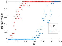
(a) $r_{1}=1$

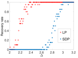
(b) $r_{1}=0.8$

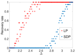
(c) $r_{1}=0.6$

Figure 2: The recovery rate of the LP relaxation versus the SDP relaxation when the input is generated according to the SSM with $n=100$ and $m=2$.

5 A stronger dual certificate

By Proposition 1, if inequalities (11) and (12) are satisfied then the partition matrix $\bar{X}$ defined by (13) is an optimal solution of Problem (2) and as a result $\bar{X}$ is an optimal solution of the K-means clustering problem. However, as evident from Proposition 4 and Figure 2, our proximity condition given by inequalities (11) and (12) are overly conservative. In the following we present a simple algorithm that leads to significantly better recovery guarantees.

Recall that in the last step of the proof of Proposition 1, our task is to identify conditions under which inequalities (26) and (27) can be satisfied. In the proof we let $\bar{\lambda}_{ijk}=0$ for all $(i,j,k)\in\Gamma_{1}$ and $\bar{\lambda}_{ijk}=0$ for all $(i,j,k)\in\Gamma_{2}$, which in turn gives us inequalities (26) and (27). As we show in the following, a careful selection of these multipliers will lead to significantly better recovery results. Define

$$\gamma_{ij}:=2\underset{k\in\Gamma_{2}}{\mathchoice{{\vbox{\hbox{$\textstyle-$ }}\kern-9.7222pt}}{{\vbox{\hbox{$\scriptstyle-$ }}\kern-8.11111pt}}{{\vbox{\hbox{$\scriptscriptstyle-$ }}\kern-6.19444pt}}{{\vbox{\hbox{$\scriptscriptstyle-$ }}\kern-5.13889pt}}\!\sum}{\min\{r_{2}d_{ik}+d^{\text{in}}_{j},r_{2}d_{jk}+d^{\text{in}}_{i}\}}-2d_{ij}-2\eta,\quad\forall i<j\in\Gamma_{1},$$

and

$$\gamma_{ij}:=2\underset{k\in\Gamma_{1}}{\mathchoice{{\vbox{\hbox{$\textstyle-$ }}\kern-9.7222pt}}{{\vbox{\hbox{$\scriptstyle-$ }}\kern-8.11111pt}}{{\vbox{\hbox{$\scriptscriptstyle-$ }}\kern-6.19444pt}}{{\vbox{\hbox{$\scriptscriptstyle-$ }}\kern-5.13889pt}}\!\sum}{\min\{r_{1}d_{ik}+d^{\text{in}}_{j},r_{1}d_{jk}+d^{\text{in}}_{i}\}}-2d_{ij}-2\frac{r_{1}}{r_{2}}\eta,\quad\forall i<j\in\Gamma_{2}.$$

We define $\gamma_{ji}:=\gamma_{ij}$ for all $i<j$. Then, by the proof of Proposition 1, the partition matrix $\bar{X}$ defined by (13) is an optimal solution of Problem (2) if the following system of inequalities is feasible:

$$\sum_{k\in\Gamma_{l^{\prime}}\setminus\{i,j\}}{(\lambda_{ijk}+\lambda_{jik}-\lambda_{kij})}\leq\gamma_{ij},\quad\forall i<j\in\Gamma_{l},l\neq l^{\prime}\in\{1,2\}$$

$$\lambda_{ijk}\geq 0,\quad\forall(i,j,k)\in\Gamma_{l},l\in\{1,2\},$$ (59)

where as before we let $\lambda_{ikj}=\lambda_{ijk}$ for $j<k$. We next present a simple algorithm whose successful termination serves as a sufficient condition for feasibility of system (5):

Input: Given $\gamma_{ij}$ for all $i<j\in\Gamma_{l}$, $l\in\{1,2\}$

Output: A Boolean success

Initialize $\bar{\lambda}_{ijk}=\bar{\lambda}_{jik}=\bar{\lambda}_{kij}=0$ for all $(i,j,k)\in\Gamma_{l}$, $l\in\{1,2\}$, $\bar{r}_{ij}=\gamma_{ij}$ for all $(i,j)\in\Gamma_{l}$, $l\in\{1,2\}$ and ${\mathcal{N}}=\{(i,j)\in\Gamma_{l},l\in\{1,2\}:i<j,\;\bar{r}_{ij}<0\}$.

while ${\mathcal{N}}\neq\emptyset$, do

       set success = .false.

       select some $(i,j)\in{\mathcal{N}}$

       for each $k\in\Gamma_{l}\setminus\{i,j\}$, do

             let $\omega=\min\{-\bar{r}_{ij},\bar{r}_{ik},\bar{r}_{jk}\}$.

             if $\omega\leq 0$, then cycle

             update $\bar{r}_{ik}\leftarrow\bar{r}_{ik}-\omega$, $\bar{r}_{jk}\leftarrow\bar{r}_{jk}-\omega$, and $\bar{r}_{ij}\leftarrow\bar{r}_{ij}+\omega$

             update $\bar{\lambda}_{kij}\leftarrow\bar{\lambda}_{kij}+\omega$, $\bar{\lambda}_{kji}\leftarrow\bar{\lambda}_{kji}+\omega$

             if $\bar{r}_{ij}\geq 0$, then

                  update success =.true.

                   update ${\mathcal{N}}\leftarrow{\mathcal{N}}\setminus\{(i,j)\}$

                   exit the k-loop

            

      if success = .false., then return

      

Certify  1 The algorithm for constructing a dual certificate

Proposition 5.

If Algorithm Certify terminates with success = .true., then the partition matrix $\bar{X}$ defined by (13) is an optimal solution of Problem (2). Moreover, Algorithm Certify runs in $\Theta(n^{3})$ operations.

Proof.

We prove that the system defined by all inequalities in system (5) with $l=1$ is feasible; the proof for $l=2$ then follows. Define

$$\bar{r}_{ij}:=\gamma_{ij}+\sum_{k\in\Gamma_{2}\setminus\{i,j\}}{(\bar{\lambda}_{kij}-\bar{\lambda}_{ijk}-\bar{\lambda}_{jik})},\quad\forall i<j\in\Gamma_{1}.$$ (60)

Then the system defined by all inequalities in system (5) with $l=1$ can be equivalently written as:

$$\bar{r}_{ij}\geq 0,\quad\forall i<j\in\Gamma_{1},\quad\bar{\lambda}_{ijk}\geq 0,\quad\forall(i,j,k)\in\Gamma_{1}.$$ (61)

If ${\mathcal{N}}=\emptyset$, then by letting $\bar{\lambda}_{ijk}=\bar{\lambda}_{jik}=\bar{\lambda}_{kij}=0$ for all $(i,j,k)\in\Gamma_{1}$, we obtain a feasible solution and the algorithm terminates with success = .true.. Hence, suppose that ${\mathcal{N}}\neq\emptyset$; that is, the initialization step violates inequalities $\bar{r}_{ij}\geq 0$ for all $(i,j)\in{\mathcal{N}}$. Consider an iteration of the algorithm for some $(\bar{i},\bar{j})\in{\mathcal{N}}$; we claim that if this iteration is completed with success = .true., all nonnegative $\bar{r}_{ij}$, $i<j\in\Gamma_{1}$ remain nonnegative (even though their values may decrease), and we will have $\bar{r}_{\overline{ij}}\geq 0$. Since the value of $\bar{\lambda}$ does not decrease over the course of the algorithm, this in turn implies that if the algorithm terminates with success = .true., $(\bar{\lambda},\bar{r})$ is feasible for system (61). To see this, consider some $\bar{k}\in\Gamma_{1}\setminus\{\bar{i},\bar{j}\}$ for which we have $\omega=\min\{-\bar{r}_{\overline{ij}},\bar{r}_{\overline{ik}},\bar{r}_{\overline{jk}}\}>0$. Notice that variable $\bar{\lambda}_{\overline{kij}}$ (which is equal to $\bar{\lambda}_{\overline{kji}}$) appears only in three equations of (60) defining $\bar{r}_{\overline{ij}}$ (with positive coefficient), $\bar{r}_{\overline{ik}}$ (with negative coefficient), and $\bar{r}_{\overline{jk}}$ (with negative coefficient). Since $\bar{r}_{\bar{ik}}\geq\omega$, $\bar{r}_{\bar{jk}}\geq\omega$, and $\omega>0$, we can increase the value of $\bar{\lambda}_{\overline{kij}}$ by $\omega$ and keep the system feasible, this in turn implies that the value of $\bar{r}_{\overline{ij}}$ will increase by $\omega$, while the values of $\bar{r}_{\overline{ik}}$ and $\bar{r}_{\overline{jk}}$ decrease by $\omega$. Therefore, if the algorithm terminates with success=.true., the assignment $(\bar{\lambda},\bar{r})$ is a feasible solution for system (61). It is simple to verify that this algorithm runs in $\Theta(n^{3})$ operation. ∎

Let us now comment on the power of Algorithm Certify for recovering the planted clusters under the stochastic ball model. Since we do not have an explicit proximity condition, we are unable to perform a rigorous probabilistic analysis similar to that of Section 4. However, in dimension $m=2$, we can perform a high precision simulation as the computational cost of Algorithm Certify is very low. First, we consider the case of equal-size clusters; i.e., $r_{1}=r_{2}=1$. We set $n=20000$ and we observe that for $\Delta>2.14$, Algorithm Certify terminates with success = .true.. That is, we conjecture the following:

Conjecture 1.

Let $m\geq 2$, and suppose that the points are generated according to the SBM with equal-size clusters. If $\Delta>2.14$, then Problem (2) recovers the planted clusters with high probability.

If true, the recovery guarantee of Conjecture 1 is better than the recovery guarantee of the SDP relaxation given by (34) for $m\leq 202$. Clearly, any convex relaxation succeeds in recovering the underlying clusters only if the original problem succeeds in doing so. To this date, the recovery threshold for K-means clustering under the SBM for $m>1$ remains an open question. Let us briefly discuss special cases $m=1$ and $m=2$. In [9], the authors prove that a necessary condition for recovery of K-means clustering in dimension one is $\Delta>1+\sqrt{3}$. In the same paper, the recovery threshold of the SDP relaxation in dimension one is conjectured to be $\Delta_{0}=4$ (see Section 2.3 of [9] for a detailed discussion). In [5], the authors prove that Problem (2) recovers the planted clusters with high probability (for every $m\geq 1$), if $\Delta>1+\sqrt{3}$. It then follows that for $m=1$, the K-means clustering problem recovers the planted clusters with high probability if and only if $\Delta>1+\sqrt{3}$. For $m=2$, in [9], via numerical simulations, the authors show that K-means clustering recovers the planted clusters with high probability only if $\Delta>2.08$. If true, Conjecture 1 implies that in dimension two, the recovery thresholds for K-means clustering and the LP relaxation are fairly close. In [11], the authors prove that, if

$$\Delta<1+\sqrt{1+\frac{2}{m+2}},$$ (62)

then the SDP relaxation fails in recovering the planted clusters with high probability. They also state that “it remains unclear whether this necessary condition (i.e., inequality (62)) is only necessary for the SDP relaxation or is necessary for the K-means itself.” If true, Conjecture 1 implies that inequality (62) is not a necessary condition for the K-means clustering problem.

We further use Algorithm Certify to estimate the recovery threshold for the case with different cluster sizes, i.e. $r_{1}\neq 1$, in dimension $m=2$. Our results are depicted in Figure 3. As can be seen from the figure, the recovery guarantee given by Algorithm Certify is significantly better than that of Proposition 4. For comparison, we have also plotted the recovery threshold for the SDP relaxation given by condition (34) for different input dimensions $m$. While Figure 3 suggests that the recovery threshold of the LP as given by Algorithm Certify quickly degrades as $r_{1}$ decreases, our numerical experiments with the LP relaxation, depicted in Figure 2 for $0.6\leq r_{1}\leq 1.0$, indicates otherwise. Notice that Algorithm Certify provides a sufficient condition for feasibility of system (5). Obtaining a better sufficient condition or, if possible, a tractable necessary and sufficient condition for the feasibility of system (5) remains an open question.

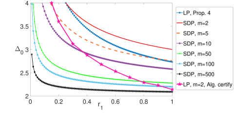
Figure 3: Comparing the recovery threshold $\Delta_{0}$ of the LP relaxation versus the SDP relaxation for K-means clustering when the input is generated according to the SBM.

6 A Counter example for the tightness of the LP relaxation

As we discussed in previous sections, in almost all our experiments with both synthetic and real-world data sets, Problem (2) is tight; i.e., its optimal solution is a partition matrix. In particular, a large number of our experiments are done under the SBM. Hence, it is natural to ask whether the LP relaxation is tight with high probability under reasonable generative models. In the following we present a family of inputs for which the LP relaxation is never tight. This family of inputs subsumes as a special case the points generated by a variation of the SBM.

To prove our result, we make use of the following lemma, which essentially states that if several sets of points have identical optimal cluster centers, then those cluster centers are optimal for the union of all points as well:

Lemma 3.

Let $\{x^{i,l}:i\in[n_{l}],l\in[L]\}$ denote a set of $N:=\sum_{l\in[L]}{n_{l}}$ points in ${\mathbb{R}}^{m}$ for some $n_{1},\dots,n_{L},L\in\mathbb{N}$, with $n_{1},\dots,n_{L},L\geq 1$. For each $l\in[L]$, consider an optimal solution of Problem (1) for clustering the $n_{l}$ points $\{x^{i,l}\}_{i=1}^{n_{l}}$ and denote by $\bar{c}^{l}\in{\mathbb{R}}^{K}$ the vector with entries equal to the $K$ centers of the optimal clusters. If $\bar{c}^{l}=\bar{c}^{l^{\prime}}$ for all $l,l^{\prime}\in[L]$, then there exists an optimal solution of Problem (1) for clustering the entire set of $N$ points with cluster centers vector $\bar{c}\in{\mathbb{R}}^{K}$ satisfying $\bar{c}^{l}=\bar{c}$ for all $l\in[L]$.

Proof.

Let $\{y^{i}\}_{i=1}^{n}$ denote a set of $n$ points in ${\mathbb{R}}^{m}$ that we would like to put into $K$ clusters and denote by $c\in{\mathbb{R}}^{K}$ the vector of cluster centers. We start by reformulating Problem (1) as follows:

$$\min_{c\in{\mathbb{R}}^{K}}\sum_{i=1}^{n}{\min\Big{\{}\lVert y^{i}-c_{1}\rVert_{2}^{2},\cdots,\lVert y^{i}-c_{K}\rVert_{2}^{2}\Big{\}}}.$$ (63)

Notice that by solving Problem (63) one directly obtains a vector of optimal cluster centers and subsequently can assign each point $y^{i}$ to a cluster at which $\min\Big{\{}\lVert y^{i}-c_{1}\rVert_{2}^{2},\cdots,\lVert y^{i}-c_{K}\rVert_{2}^{2}\Big{\}}$ is attained. Now for each $l\in[L]$, define

$$f_{l}(c):=\sum_{i=1}^{n_{l}}{\min\Big{\{}\lVert x^{i,l}-c_{1}\rVert_{2}^{2},\cdots,\lVert x^{i,l}-c_{K}\rVert_{2}^{2}\Big{\}}}.$$

It then follows that the K-means clustering problem for clustering the $n_{l}$ points $\{x^{i,l}\}_{i=1}^{n_{l}}$ for some $l\in[L]$ can be written as:

$$\min_{c\in{\mathbb{R}}^{K}}f_{l}(c),$$ (64)

while the K-means clustering problem for the entire set of $N$ points can be written as

$$\min_{c\in{\mathbb{R}}^{K}}\sum_{l\in L}{f_{l}(c)}.$$ (65)

Clearly, $\sum_{l\in L}\min_{c\in{\mathbb{R}}^{K}}f_{l}(c)\leq\min_{c\in{\mathbb{R}}^{K}}\sum_{l\in L}{f_{l}(c)}$. Hence, if for each $l\in[L]$, there exists a minimizer $\bar{c}^{l}$ of Problem (64) such that $\bar{c}^{l}=\bar{c}^{l^{\prime}}$ for all $l,l^{\prime}\in[L]$, we conclude that $\bar{c}^{l}$ is a minimizer of Problem (65) as well. ∎

Now let us investigate the tightness of the LP relaxation defined by Problem (2). First note that by Proposition 5 in [5], if $n\leq 4$, then the feasible region of Problem (2) coincides with the convex hull of the feasible region of Problem (3). Hence, to find an instance for which the LP relaxation is not tight we must have $n\geq 5$.

Consider the following $n=5$ points in dimension $m=3$, which we refer to as the five-point input:

$$x^{1}=\Big{(}0,\frac{\sqrt{3}}{3},0\Big{)},\;x^{2}=\Big{(}\frac{1}{2},-\frac{\sqrt{3}}{6},0\Big{)},\;x^{3}=\Big{(}-\frac{1}{2},-\frac{\sqrt{3}}{6},0\Big{)},\;x^{4}=\Big{(}0,0,\frac{1}{2}\Big{)},\;x^{5}=\Big{(}0,0,-\frac{1}{2}\Big{)}.$$ (66)

In this case the vector of squared pair-wise distances $d=(d_{ij})_{1\leq i<j\leq 5}$ is given by

$$d=\Big{(}1,1,\frac{7}{12},\frac{7}{12},1,\frac{7}{12},\frac{7}{12},\frac{7}{12},\frac{7}{12},1\Big{)}.$$ (67)

By direct calculation it can be checked that the partition $\Gamma_{1}=\{1,4\}$ and $\Gamma_{2}=\{2,3,5\}$ is a minimizer of the K-means clustering problem (1) with the optimal objective value given by

$$f^{*}_{\rm Kmeans}=\frac{146}{72}>2.$$

Now consider the following matrix

$$\tilde{X}=\frac{1}{14}\begin{bmatrix}6&1&1&3&3\\ 1&6&1&3&3\\ 1&1&6&3&3\\ 3&3&3&5&0\\ 3&3&3&0&5\end{bmatrix}.$$ (68)

Notice that $\tilde{X}$ is not a partition matrix. It is simple to verify the feasibility of $\tilde{X}$ for the LP relaxation. Moreover, the objective value of Problem (2) at $\tilde{X}$ evaluates to $\hat{f}_{\rm LP}=\frac{54}{28}<2$. Denote by $f^{*}_{\rm LP}$ the optimal value of Problem (2). Since $f^{*}_{\rm LP}\leq\hat{f}_{\rm LP}<f^{*}_{\rm Kmeans}$, we conclude that for the five-point input, the LP relaxation is not tight.

Now consider the following set of points, which we will refer to as the five-ball input. Instead of $n=5$ points located at each $x^{p}$, $p\in\{1,\cdots,5\}$ defined by (66), suppose that we have $n=5n^{\prime}$ points for some $n^{\prime}\in\mathbb{N}$, $n^{\prime}\geq 1$, such that for each $p\in\{1,\ldots,5\}$, we have $n^{\prime}$ points located inside a closed ball of radius $r\geq 0$ centered at $x^{p}$. In the following we show that for $r\leq 3\times 10^{-3}$, the LP relaxation always fails in finding the optimal clusters.

Proposition 6.

Consider an instance of the five-ball input for some $r\leq 3\times 10^{-3}$. Then the LP relaxation is not tight; i.e., , the optimal value of Problem (2) is strictly smaller than that of Problem (1).

Proof.

We denote by ${\mathcal{B}}_{p}$ the index set of points located in the $p$th ball; without loss of generality, let ${\mathcal{B}}_{p}=\{(p-1)n^{\prime}+1,\cdots,pn^{\prime}\}$ for all $p\in\{1,\cdots,5\}$. Let us denote these points by $y^{j}$, $j\in{\mathcal{B}}_{p}$, $p\in\{1,\cdots,5\}$.

We start by computing an upper bound on the optimal value of the LP relaxation. Consider the matrix $\hat{X}$ defined as follows:

$$\hat{X}_{ij}=\frac{6}{14n^{\prime}},\quad\forall i,j\in{\mathcal{B}}_{p},\;p\in\{1,2,3\}$$

$$\hat{X}_{ij}=\frac{5}{14n^{\prime}},\quad\forall i,j\in{\mathcal{B}}_{p},\;p\in\{4,5\}$$

$$\hat{X}_{ij}=\frac{1}{14n^{\prime}},\quad\forall i\in{\mathcal{B}}_{p},\;j\in{\mathcal{B}}_{p^{\prime}},\;p\neq p^{\prime}\in\{1,2,3\}$$

$$\hat{X}_{ij}=\frac{3}{14n^{\prime}},\quad\forall i\in{\mathcal{B}}_{p},\;j\in{\mathcal{B}}_{p^{\prime}},\;p\in\{1,2,3\},\;p^{\prime}\in\{4,5\}$$

$$\hat{X}_{ij}=0,\quad\forall i\in{\mathcal{B}}_{p},\;j\in{\mathcal{B}}_{p^{\prime}},\;p\neq p^{\prime}\in\{4,5\}.$$

Clearly, $\hat{X}$ is not a partition matrix. First we show that $\hat{X}$ is feasible for Problem (2). The equality constraint (5) is satisfied as we have ${\rm Tr}(\hat{X})=\sum_{i\in[n]}{\hat{X}_{ii}}=3n^{\prime}(\frac{6}{14n^{\prime}})+2n^{\prime}(\frac{5}{14n^{\prime}})=2$. Equalities (6) are also satisfied since we have $\sum_{j=1}^{n}{\hat{X}_{ij}}=n^{\prime}(\frac{6}{14n^{\prime}})+2n^{\prime}(\frac{1}{14n^{\prime}})+2n^{\prime}(\frac{3}{14n^{\prime}})=1$ for all $i\in{\mathcal{B}}_{p},p\in\{1,2,3\}$, and $\sum_{j=1}^{n}{\hat{X}_{ij}}=3n^{\prime}(\frac{3}{14n^{\prime}})+n^{\prime}(\frac{5}{14n^{\prime}})+n^{\prime}(0)=1$ for all $i\in{\mathcal{B}}_{p},p\in\{4,5\}$. Hence it remains to check the validity of inequalities (7): first note that if $i\in{\mathcal{B}}_{p}$, $j\in{\mathcal{B}}_{p^{\prime}}$, $k\in{\mathcal{B}}_{p^{\prime\prime}}$ for $p\neq p^{\prime}\neq p^{\prime\prime}$, then the validity of $\hat{X}_{ij}+\hat{X}_{ik}\leq\hat{X}_{ii}+\hat{X}_{jk}$ follows from the validity of inequalities  (7) at $\tilde{X}$ defined by (68). If $i,j,k\in{\mathcal{B}}_{p}$, $p\in\{1,2,3\}$, then $\hat{X}_{ij}+\hat{X}_{ik}=\frac{6}{14n^{\prime}}+\frac{6}{14n^{\prime}}\leq\frac{6}{14n^{\prime}}+\frac{6}{14n^{\prime}}=\hat{X}_{ii}+\hat{X}_{jk}$ for all $i\neq j\neq k$, $j<k$. If $i,j,k\in{\mathcal{B}}_{p}$, $p\in\{4,5\}$, then $\hat{X}_{ij}+\hat{X}_{ik}=\frac{5}{14n^{\prime}}+\frac{5}{14n^{\prime}}\leq\frac{5}{14n^{\prime}}+\frac{5}{14n^{\prime}}=\hat{X}_{ii}+\hat{X}_{jk}$ for all $i\neq j\neq k$, $j<k$. The remaining cases, i.e., when two of the points are in the same ball, while the third point is in a different ball, can be checked in a similar fashion.

Denote by $d^{r}_{ij}$ , $1\leq i<j\leq n$, the vector of squared pairwise distances. We have:

$$d^{r}_{ij}\leq 4r^{2},\quad\forall i,j\in{\mathcal{B}}_{p},p\in\{1,\ldots,5\},$$

$$d^{r}_{ij}\leq(1+2r)^{2},\quad\forall i\in{\mathcal{B}}_{p},j\in{\mathcal{B}}_{p^{\prime}},\forall p\neq p^{\prime}\in\{1,2,3\},\;{\rm or}\;p\neq p^{\prime}\in\{4,5\},$$

$$d^{r}_{ij}\leq\Big{(}\sqrt{\frac{7}{12}}+2r\Big{)}^{2},\quad\forall i\in{\mathcal{B}}_{p},j\in{\mathcal{B}}_{p^{\prime}},\forall p\in\{1,2,3\},p^{\prime}\in\{4,5\}.$$

Hence, an upper bound $\hat{g}_{\rm LP}(r)$ on the optimal value of Problem (2) is given by

$$g^{*}_{\rm LP}(r) \leq 6\binom{n^{\prime}}{2}\frac{6}{14n^{\prime}}(4r^{2})+4\binom{n^{\prime}}{2}\frac{5}{14n^{\prime}}(4r^{2})+6n^{\prime 2}\frac{1}{14n^{\prime}}(1+2r)^{2}+12n^{\prime 2}\frac{3}{14n^{\prime}}\Big{(}\sqrt{\frac{7}{12}}+2r\Big{)}^{2}$$

$$=n^{\prime}\Big{(}\frac{54}{28}+20r^{2}+12(\frac{\sqrt{21}+1}{7})r-8\frac{r^{2}}{n^{\prime}}\Big{)}\leq\Big{(}\frac{54}{28}+10r\Big{)}n^{\prime}:=\hat{g}_{\rm LP}(r),$$ (69)

where the last inequality follows since by assumption $r\leq 3\times 10^{-3}$, and where $g^{*}_{\rm LP}(r)$ denotes the optimal value of Problem (2) for the five-ball input.

Denote by $g^{*}_{\rm Kmeans}(r)$ the optimal value of the K-means clustering problem (1) for the five-ball input. Next, we obtain a lower bound on $g^{*}_{\rm Kmeans}(r)$, and show that this value is strictly larger than $\hat{g}_{\rm LP}(r)$ defined by (69) for any $0\leq r\leq 3\times 10^{-3}$, implying that Problem (2) is not tight. To this end, first consider the case with $r=0$. Define the set of points $Y^{l}:=\{y^{l},y^{n^{\prime}+l},y^{2n^{\prime}+l},y^{3n^{\prime}+l},y^{4n^{\prime}+l}\}$ for all $l\in[n^{\prime}]$. Notice that since $r=0$, we have $Y^{l}=Y^{l^{\prime}}$ for all $l,l^{\prime}\in[n^{\prime}]$. For each $l\in[n^{\prime}]$, consider the K-means clustering problem with $K=2$ for five input points $Y^{l}$, and denote the optimal cluster centers by $(c^{l}_{1},c^{l}_{2})$. We then have $(c^{l}_{1},c^{l}_{2})=(c_{1},c_{2})$ for all $l\in[n^{\prime}]$, where $(c_{1},c_{2})$ denotes the optimal cluster centers for the five-point input (66). Therefore, by Lemma 3, we conclude that an optimal cluster centers for the five-ball input with $r=0$, coincides with an optimal cluster centers for the five-point input. This in turn implies that

$$g^{*}_{\rm Kmeans}(0)=n^{\prime}f^{*}_{\rm Kmeans}=\frac{146}{72}n^{\prime}.$$ (70)

Now let us consider the five-ball input for some $r>0$. We observe that

$$\sqrt{d^{r}_{ij}}\geq\sqrt{d^{0}_{ij}}-2r,\quad\forall 1\leq i<j\leq n.$$

Since $d^{0}_{ij}\leq 1$ for all $1\leq i<j\leq n$, we have

$$d^{r}_{ij}\geq d^{0}_{ij}-4r,\quad\forall 1\leq i<j\leq n.$$

Therefore, for every partition matrix $X$ we compute

$$\sum_{i,j\in[n]}{d^{r}_{ij}X_{ij}}\geq\sum_{i,j\in[n]}{d^{0}_{ij}X_{ij}}-4r\sum_{i,j\in[n]}{X_{ij}}=\sum_{i,j\in[n]}{d^{0}_{ij}X_{ij}}-20rn^{\prime},$$

where the last equality follows from constraints (6). Hence, taking the minimum over all partition matrices on both sides and using (70), we deduce that

$$g^{*}_{\rm Kmeans}(r)\geq g^{*}_{\rm Kmeans}(0)-20rn^{\prime}=\Big{(}\frac{146}{72}-20r\Big{)}n^{\prime}.$$ (71)

From (69) and (71) it follows that by choosing

$$r<\frac{\frac{146}{72}-\frac{54}{28}}{30},$$

we get $g^{*}_{\rm LP}(r)<g^{*}_{\rm Kmeans}(r)$ and this completes the proof. ∎

As a consequence of Proposition 6, we find that the LP relaxation is not tight for a variant of the SBM:

Corollary 1.

Let $r\leq 3\times 10^{-3}$. Suppose that the points are generated in ${\mathbb{R}}^{m}$, for some $m\geq 3$ according to any generative model consisting of five measures $\mu_{p}$, $p=1,\dots,5$, each supported in the ball $B((x^{p},0,\dots,0),r)$, where $x^{p}$ is defined by (66). Then Problem (2) is not tight.

Recall that in all our previous numerical experiments with synthetic and real-world data sets, the LP relaxation outperforms the SDP relaxation. That is, the optimal value of the LP is always at least as large as that of the SDP. Hence, one wonders whether such a property can be proved in a general setting. Interestingly, the stochastic model defined in Corollary 1 provides the first counter example, which we illustrate via a numerical experiment. We consider the stochastic model defined in Corollary 1, where we assume the points supported by each ball are sampled from a uniform distribution. We set $m=3$ and generate $n^{\prime}=20$ points in each of the five balls to get a total of $n=100$ points. Moreover we set ball radii $r\in[0.0:0.01:0.5]$ and for each fixed $r$ we generate 20 random instances. Our results are depicted in Figure 4, where as before we compare the LP, i.e., Problem (2), with the SDP, i.e., Problem (PW), with respect to their tightness rate and average relative gap. Recall that the relative gap is defined as $g_{\rm rel}=\frac{f_{\rm LP}-f_{\rm SDP}}{f_{\rm LP}}\times 100$, where $f_{\rm LP}$ and $f_{\rm SDP}$ denote the optimal values of the LP and the SDP, respectively. That is, a negative relative gap means that the SDP relaxation is stronger than the LP relaxation. As can be seen from the figure, while the SDP is never tight, for $r\lesssim 0.15$, we often have $f_{\rm SDP}>f_{\rm LP}$.

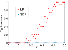
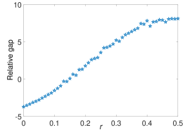
Figure 4: Comparing the strength of the LP relaxation versus the SDP relaxation for K-means clustering when the input is generated according to the stochastic five-ball input with $n=100$ and $m=3$.

We conclude this paper by remarking that the family of examples we constructed in this section are very special and our numerical experiments with real-world data sets suggest that such special configurations do not appear in practice. Hence, it is highly plausible that one can establish the tightness of the LP relaxation under a fairly general family of inputs. We leave this as an open question.

References

- [1] MOSEK 9.2, 2019. http://docs.mosek.com/9.0/faq.pdf.
- [2] D. Aloise, A. Deshpande, P. Hansen, and P. Popat. NP-hardness of Euclidean sum-of-squares clustering. Machine Learning, 75:245–248, 2009.
- [3] P. Awasthi, A. S. Bandeira, M. Charikar, R. Krishnaswamy, S. Villar, and R. Ward. Relax, no need to round: Integrality of clustering formulations. Proceedings of the 2015 Conference on Innovations in Theoretical Computer Science, 165:191–200, 2015.
- [4] J. Czyzyk, M. P. Mesnier, and J. J. More. The NEOS server. IEEE Journal on Computational Science and Engineering, 5(3):68 –75, 1998.
- [5] A. De Rosa and A. Khajavirad. The ratio-cut polytope and K-means clustering. SIAM Journal on Optimization, 32(1):173–203, 2022.
- [6] Dheeru Dua, Casey Graff, et al. UCI machine learning repository. URL http://archive. ics. uci. edu/ml, 2017.
- [7] Z. Friggstad, M. Rezapour, and Salavatipour M. R. Local search yields a PTAS for K-means in doubling metrics. SIAM Journal on Computing, 48(2):452–480, 2019.
- [8] Gurobi Optimization, LLC. Gurobi Optimizer Reference Manual, 2021. URL: https://www.gurobi.com.
- [9] T. Iguchi, D. G. Mixon, J. Peterson, and S. Villar. Probably certifiably correct K-means clustering. Mathematical Programming, 165:605–642, 2017.
- [10] T. Kanungo, D.M. Mount, N.S. Netanyahu, C.D. Piatko, R. Silverman, and A.Y. Wu. A local search approximation algorithm for K-means clustering. Proceedings of the 18th Annual ACM Symposium on Computational Geometry, pages 10–18, 2002.
- [11] X. Li, Y. Li, S. Ling, T. Strohmer, and K. Wei. When do birds of a feather flock together? K-means, proximity, and conic programming. Mathematical Programming, 179:295–341, 2020.
- [12] S. Lloyd. Least squares quantization in PCM. IEEE Transactions on Information Theory, 28(2):129 –137, 1982.
- [13] M. Mahajan, P. Nimbhorkar, and K. Varadarajan. The planar K-means problem is NP-hard. In WALCOM: Algorithms and Computation, pages 274–285. Springer Berlin Heidelberg, 2009.
- [14] O.L. Mangasarian. Uniqueness of solution in linear programming. Linear Algebra and its Applications, 25:151–162, 1979.
- [15] D. G. Mixon, S. Villar, and R. Ward. Clustering subgaussian mixtures by semidefinite programming. Information and Inference: A Journal of the IMA, 6(4):389–415, 2017.
- [16] J Peng and Y Wei. Approximating K-means-type clustering via semidefinite programming. SIAM Journal on Optimization, 18(1):186–205, 2007.
- [17] J. Peng and Y. Xia. A New Theoretical Framework for K-Means-Type Clustering, pages 79–96. Springer Berlin Heidelberg, 2005.
- [18] V. Piccialli, A. M. Sudoso, and A. Wiegele. SOS-SDP: An exact solver for minimum sum-of-squares clustering. INFORMS Journal on Computing, 34(4):2144–2162, 2022.
- [19] M. N. Prasad and G. A. Hanasusanto. Improved conic reformulations for K-means clustering. SIAM Journal on Optimization, 28(4):3105–3126, 2018.
- [20] R. Vershynin. High-dimensional probability: An introduction with applications in data science, volume 47. Cambridge University Press, 2018.