Deep Room Impulse Response Completion

Abstract

Rendering immersive spatial audio in virtual reality (VR) and video games demands a fast and accurate generation of room impulse responses (RIRs) to recreate auditory environments plausibly. However, the conventional methods for simulating or measuring long RIRs are either computationally intensive or challenged by low signal-to-noise ratios. This study is propelled by the insight that direct sound and early reflections encapsulate sufficient information about room geometry and absorption characteristics. Building upon this premise, we propose a novel task termed ”RIR completion,” aimed at synthesizing the late reverberation given only the early portion (50 ms) of the response. To this end, we introduce DECOR, Deep Exponential Completion Of Room impulse responses, a deep neural network structured as an autoencoder designed to predict multi-exponential decay envelopes of filtered noise sequences. The interpretability of DECOR’s output facilitates its integration with diverse rendering techniques. The proposed method is compared against an adapted state-of-the-art network, and comparable performance shows promising results supporting the feasibility of the RIR completion task. The RIR completion can be widely adapted to enhance RIR generation tasks where fast late reverberation approximation is required.

1 Introduction

Generating room impulse responses (RIRs) is a well-studied topic with many applications and proposed solutions. A recent application area is virtual acoustics rendering for computer games and augmented and virtual reality (AR/VR), where dynamic sound scenes require realistic and real-time RIRs. Generating RIRs accurately and in real-time remains an open task. This paper proposes a new task, RIR completion, for fast RIR generation and presents a lightweight deep learning approach that solves this RIR completion task.

1.1 Background

Despite extensive work in RIR generation, challenges remain in broadband accuracy, computational complexity, and real-time synthesis. Room acoustics modeling, such as wave-based and geometrical acoustics, aims to simulate acoustic waves accurately, given a 3D representation of the room with acoustic material assigned to its surfaces. Geometrical acoustics (GA) [1, 2, 3, 4, 5, 6, 7, 8] which model sound propagation as a ray, accurately simulates the behavior of high frequencies, but fails to capture wave phenomena such as diffraction especially at low frequencies. Wave-based methods solve the wave equation numerically with methods such as the Finite Difference Time-Domain (FDTD) method [9, 10], Finite Element Method (FEM), and Boundary Element Method (BEM). Wave-based methods are computationally expensive because complexity exponentially increases with respect to frequency, and quantization and boundary errors cause inaccuracies. The computational complexity of both methods increases considerably with respect to the length of the simulated RIR signal.

Generating broadband RIRs with one single approach is computationally expensive. Therefore, hybrid room acoustics modeling methods for combining the early and the late reverberation, or the high-frequency and low-frequency content from different techniques have been proposed over the past few decades [11, 12, 13].

On the other hand, algorithmic reverberation techniques generate RIRs using parameterized signal processing methods [14, 15, 16, 17, 18, 19], typically for musical reverb with an emphasis on real-time processing and artistic control. These methods’ efficiency relies on approximating the early and late reverberation with different accuracy to match perceptually plausible reverberation while reducing the processing cost.

1.2 RIR Completion

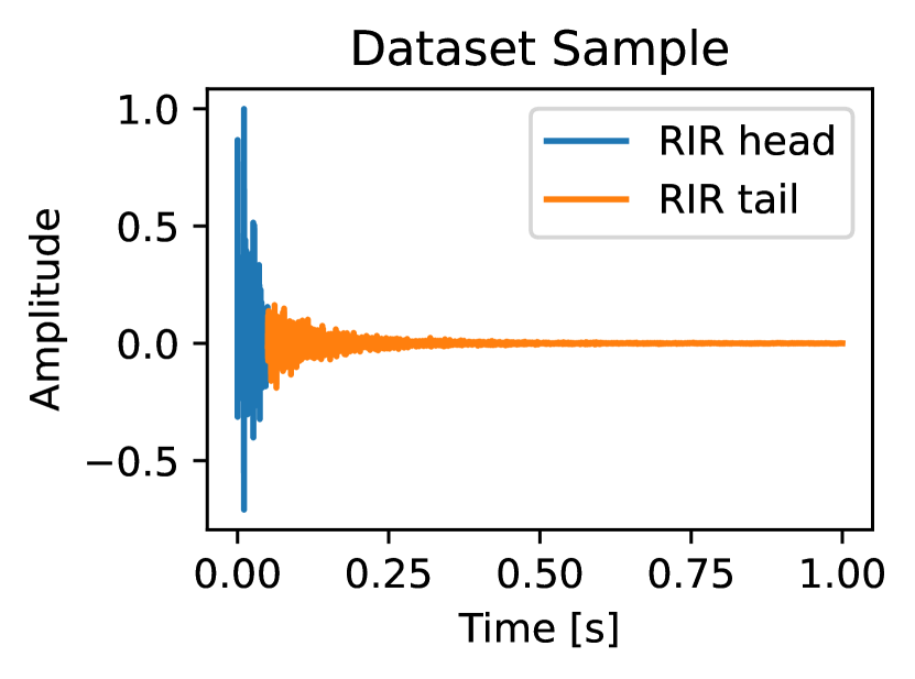
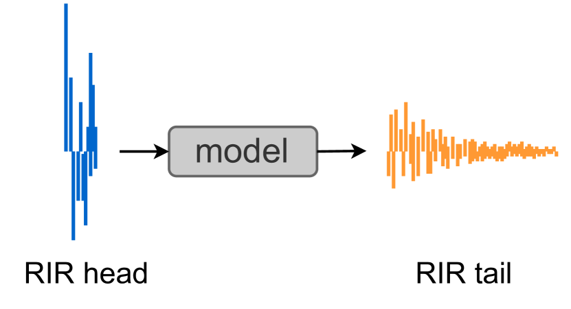
We present the task of RIR completion, where given only the early part of the time-domain RIR (head), the objective is to predict the rest of the RIR sequence (tail), as depicted in Figure 1. The motivation for RIR completion is to reduce the computation time and cost of RIR synthesis by obtaining a short RIR head with conventional methods and then using a fast procedure to complete the RIR tail. For estimated or measured RIRs, the early reflections are retrieved more reliably due to a higher signal-to-noise ratio.

Our primary assumption is that the direct sound and the early reflections in the RIR head contain enough information about the room geometry and acoustic material properties to predict the late reverberation. In the image source method [2, 3], the RIR is synthesized by summing each reflected wavefront that arrives at the receiver with the appropriate distance delay and attenuation. This means that within a short time after excitation, many, if not all, of the room surfaces have reflected energy to the receiver. For example, in a medium-sized rectangular room with dimensions $$5\text{\,}\mathrm{m}$\times$5\text{\,}\mathrm{m}$\times$3\text{\,}\mathrm{m}$$, all reflections of second-order and lower, and up to some fourth-order arrive at the receiver within $50\text{\,}\mathrm{ms}$.

Figure 1: Left: example RIR from the Motus  [20] dataset, divided at 50 ms into its head and tail components. Right: RIR completion task – take the RIR head and predict the tail.

To our knowledge, the task of RIR completion, i.e., inferring the RIR tail from just the RIR head, has not been explored. We list our contributions as follows:

1. We propose a machine-learning-based approach for the task of RIR completion.

2. We evaluate our proposed method against a state-of-the-art RIR generation approach and show our method achieves a similar performance with a much smaller network.

The following section provides an overview of related work in RIR generation using deep learning and examples of similar inverse problems that support the feasibility of our task.

Figure 2: DECOR overview. The RIR head $\bm{x}$ is passed through an autoencoder architecture. Within the decoder, we predict multi-exponential decay envelopes $\bm{y_{i}}$, which are used to shape filtered noise sequences $\bm{s_{i}}$. The shaped noise sequences are combined to form the RIR tail $\bm{\hat{h}}$.

1.3 Related Work

More recently, the application of deep learning to RIR generation in room acoustics modeling and blind estimation has yielded promising results. To that point, the work of [21] demonstrates that variational autoencoders, and more broadly, deep learning approaches, are well suited for sample-by-sample RIR generation given any informative input (reverberant recordings, geometry, etc.).

Specifically, deep learning approaches for room acoustics modeling have been proposed: Ratnarajah et al. [22] proposed a graph convolution neural network that synthesizes an RIR from the graph representation of an indoor 3D scene. Physics-Informed Neural Networks (PINNs), neural networks constrained by the wave equation, have been proposed for sound field reconstruction and RIR generation [23, 24] as an alternative to both traditional wave-based methods and data-driven deep learning methods. Neural representational methods (NeRFs) that encode a room to a continuously queryable representation have been proposed by Luo et al. [25] and Richard et al. [26] to predict the RIR given the coordinates of the source and receiver. These examples, however, have limited scope, as they either require precomputing the mesh-to-graph conversion or generating RIRs for one room only.

In blind estimation, room parameters or the full RIR signal are inferred from non-RIR input such as reverberant speech recording [27], images [28, 29], or videos of the room [30]. For example, Koo et al. [31] proposed a U-Net model to predict a sample-by-sample RIR given a reverberant singing recording. Similarly, Steinmetz et al. [32] proposed the Filtered Noise Shaping (FiNS) network that is a 1D-convolution autoencoder network that takes reverberant speech and predicts a sample-by-sample early part of the RIR ($50\text{\,}\mathrm{ms}$) and time domain envelopes that shape filtered noise for the late reverberation. We adapt FiNS as a baseline later in the evaluation section.

Lastly, work in geometry prediction using room impulse responses has been explored before, which further supports the tractability of our proposed RIR completion task. Moore [33], Markovic [34], and Kuster [35] used analytical methods to estimate room geometry or volume from a single-channel RIR. Later on, Yu and Kleijn [36] proposed a CNN to estimate the geometry of a room and reflection coefficients from a single RIR. These inverse methods indicate that the RIR contains retrievable information about its corresponding room and scene and thus motivate using the RIR head to predict the RIR tail.

The paper is organized as follows: Section 2 describes our proposed neural network and experimental setup in detail. Section 3 presents the evaluation of our proposed method and compares it to a state-of-the-art RIR generation baseline adapted to the RIR completion task. Section 4 discusses our method’s performance on this new task and presents several applications of our work. Section 5 concludes the paper.

2 Methods

In this section, we present our neural network DECOR, Deep Exponential Completion Of Room impulse responses, that takes the RIR time domain head and predicts the RIR tail, i.e.,

$$\Phi:\mathbf{h}_{[$0\text{\,}\mathrm{s}$,\,$50\text{\,}\mathrm{ms}$]}\xrightarrow{}\mathbf{h}_{[$50\text{\,}\mathrm{ms}$,\,$1\text{\,}\mathrm{s}$]}\,.$$ (1)

First, we present the encoder-decoder structure of DECOR, shown in Figure 2, with a detailed explanation of the acoustics-informed decoder. Then, we discuss the loss function, datasets, and experimental setup details that were used in the training of the model.

2.1 Encoder

We modify the encoder structure from the FiNS model [32] which originally took a few seconds of reverberant speech, for the short RIR head input. The DECOR time-domain encoder takes the first $50\text{\,}\mathrm{ms}$ of the RIR sampled at $48\text{\,}\mathrm{kHz}$ as the input $\bm{x}\in\mathbb{R}^{2400}$, and performs a series of strided 1D convolutions and skip connections via the encoding block described in [32]. Nine encoding blocks progressively downsample $\bm{x}$. The output is passed through an adaptive 1D pooling layer and then through a single linear layer to obtain the latent vector $\bm{z}$ with desired embedding length $k=128$.

2.2 Decoder

We designed the decoder with strong room acoustics inductive bias to minimize the model size and amount of training data while maximizing expressive power. The decoder of DECOR is based on the exponentially decaying white noise model of reverberation, described by Moorer [16]. Due to the stochastic nature of late reverberation, the room impulse response $h(n)$ can be described as stochastic white noise $w(n)$ enveloped by a sum of $N$ exponential decays

$$h(n)=w(n)\sum_{j=1}^{N}{a_{j}e^{-b_{j}n}}\,,$$ (2)

where $a_{j}$ and $b_{j}$ are the initial amplitude of the decay and decay rate, respectively.

This impulse response representation can be further broken down into frequency bands $i=1,...,M$ to capture frequency-dependent decay,

$$h(n)=\sum_{i=1}^{M}{h_{i}(n)}=\sum_{i=1}^{M}s_{i}(n)\ {\sum_{j=1}^{N}{a_{ij}e^{-b_{j}n}}}\,,$$ (3)

where $s_{i}(n)$ is band-limited noise corresponding to the different frequency bands. For a discrete-time sequence of length $T$, we omit $n$ and simplify the notation to

$$\bm{h}=\sum_{i=1}^{M}{\bm{s}_{i}\odot\bm{y}_{i}}\,,$$ (4)

where $\bm{y}_{i}\in\mathbb{R}^{1\times T}$ is the time-domain envelope for the filtered white noise sequence $\bm{s}_{i}\in\mathbb{R}^{1\times T}$ and $\odot$ denotes element-wise multiplication.

The time-domain envelope $\bm{y}_{i}$ can be expressed as a linear combination of exponential decay envelopes in vector notation

$$\bm{y}_{i}=\bm{a}_{i}\bm{E}\,,$$ (5)

where $\bm{a}_{i}\in\mathbb{R}^{1\times N}$ and exponential decay envelopes $\bm{E}$ is computed for $N$ decay rates $\bm{b}\in\mathbb{R}^{N}$ for time sequence $\bm{n}\in\mathbb{R}^{T}$ i.e.,

$$\bm{E}:=e^{-\bm{b}\bm{n}^{\intercal}}\in\mathbb{R}^{N\times T}\,.$$ (6)

The proposed decoder is depicted in Figure 3. It constructs the time-domain envelopes $\bm{Y}$ by predicting the decay envelope amplitude values $\bm{A}$ and multiplying them with the exponential decay envelopes $\bm{E}$.

Figure 3: Decoder structure. The latent vector $\bm{z}$ is concatenated with a random noise vector $\bm{v}$ and fed through a multihead MLP, producing the log-amplitudes $\bm{A}^{\prime}$ and mask $\sigma(\bm{C}^{\prime})$. The exponential decay envelopes $\bm{E}$ are constructed separately, using the learned decay rates $\bm{b}$. The exponential decay amplitude matrix is calculated as $\bm{A}=e^{\bm{A}^{\prime}}\odot\sigma(\bm{C}^{\prime})$ and multiplied with $\bm{E}$ to output the time domain decay envelopes $Y$.

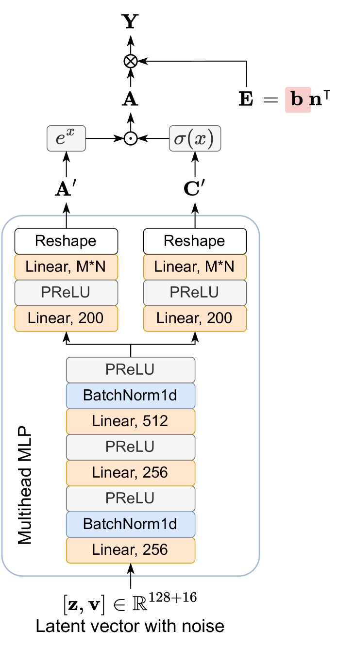
The decay envelope amplitudes $\bm{A}$ are predicted as shown in Figure 3. A multihead MLP with seven hidden layers takes the latent vector $\bm{z}$ concatenated with a noise vector $\bm{v}$ of length $d$ and outputs two matrices $\bm{A}^{\prime}$ and $\bm{C}^{\prime}$. The element-wise product of the exponential of $\bm{A}^{\prime}$ and the mask $\bm{C}=\sigma(\bm{C}^{\prime})$ gives the decay envelope amplitude matrix

$$\bm{A}=e^{\bm{A}^{\prime}}\odot\sigma(\bm{C^{\prime}})\,,$$ (7)

where $\sigma(\cdot)$ is the sigmoid function and $\bm{C}=\sigma(\bm{C}^{\prime})=\{c_{ij}\mid 0\leq c_{ij}\leq 1\}$.

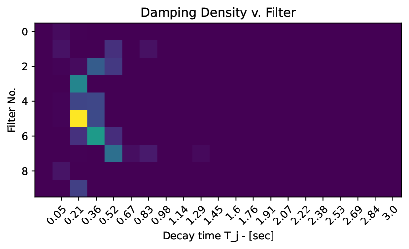
We found that learning a logarithmic representation $\bm{A}^{\prime}$ and a separate sigmoid mask, achieved better results than learning $\bm{A}$ directly. Due to the logarithmic representation, the predicted values $\bm{A}^{\prime}$ are more evenly distributed across a smaller range, thus facilitating model training. Similar observations were previously reported in [37]. The separate prediction of $\bm{C}^{\prime}$ and application of the sigmoid function yield masks that enforce close to zero amplitudes for non-active decays. Combining both strategies helped to enforce sparsity in $\bm{A}$, see Fig. 4.

The exponential decay envelopes $\bm{E}$ is then constructed from $\bm{b}$ and $\bm{n}$ using Eq. (6). The learnable parameter $\bm{b}=\{b_{j}\mid b_{j}=\ln(10^{-3})/T_{j}\}\in\mathbb{R}^{N}$ is initialized before training and fixed during inference, with $T_{j}$ being the T60 decay time of the $j$th slope. In our final model, we initialized $N=20$ decay times, linearly sampled from the range $0.05\text{\,}\mathrm{s}3.0\text{\,}\mathrm{s}$. The envelope matrix $\bm{E}$ is calculated for a $950\text{\,}\mathrm{ms}$ time sequence corresponding to the RIR tail, i.e., $\bm{n}=[0.05,0.05+1/f_{\textrm{s}},...,1.0]\in\mathbb{R}^{T}$, with sequence length $T=45600$ at sampling frequency $f_{\textrm{s}}=$48\text{\,}\mathrm{kHz}$.$

Taking a similar filtered noise approach as in FiNS [32], we construct a filterbank of $M$ learnable FIR filters that processes a Gaussian white noise signal $\bm{w}\in\mathbb{R}^{T}$ into $M$ filtered noise signals $\bm{S}=[\bm{s}_{1},\bm{s}_{2},...\bm{s}_{M}]$, see Fig. 2. We initialize the learnable filterbank with $M=10$ FIR octave band filters of order $P=1023$. Finally, the RIR signal is constructed from the element-wise product of the time-domain envelopes and the filtered noise signals

$$\bm{H}=\bm{Y}\odot\bm{S}\,,$$ (8)

where the rows of $\bm{H}\in\mathbb{R}^{M\times T}$ are filtered noise signals weighted with the learned envelopes. A last linear layer linearly combines the rows of $\bm{H}$ to return the full-band predicted RIR tail

$$\bm{\hat{h}}=\bm{w}^{\intercal}_{\textrm{Linear}}\bm{H}\,.$$ (9)

2.3 Experimental Setup

In the following, we present the loss function, training dataset, and training parameters.

2.3.1 Loss Function

A multiresolution short-time Fourier transform (MSTFT) loss function [38, 32] was used to train and evaluate the model. The MSTFT loss function $\mathcal{L}_{\text{MSTFT}}(\hat{h},h)$ between the predicted RIR $\hat{h}(n)$ and the true RIR $h(n)$ is given as the sum of $R$ STFT losses with different STFT resolutions, i.e.,

$$\mathcal{L}_{\text{MSTFT}}(\hat{h},h)=\sum_{r=1}^{R}{\mathcal{L}_{\text{sc},\,r}(\hat{h},h)+\mathcal{L}_{\text{sm},\,r}(\hat{h},h)}\,.$$ (10)

The STFT loss is the sum of the spectral convergence loss

$$\mathcal{L}_{\text{sc},\,r}(\hat{h},h)=\frac{\norm{\lvert\text{STFT}_{r}(h)\rvert-\lvert\text{STFT}_{r}(\hat{h})\rvert}_{F}}{\norm{\lvert\text{STFT}_{r}(h)\rvert}_{F}}$$ (11)

and the spectral log-magnitude loss

$$\begin{split}\mathcal{L}_{\text{sm},\,r}(\hat{h},h)=\frac{1}{N}\lVert&\log{(\lvert\text{STFT}_{r}(h)\rvert)}\\ &-\log{(\lvert\text{STFT}_{r}(\hat{h})\rvert)}\rVert_{1}\,,\end{split}$$ (12)

where $\norm{\cdot}_{F}$ is the Frobenius norm, and $\norm{\cdot}_{1}$ is the $L_{1}$ norm.

During our training we used $R=4$ resolutions, with window sizes $[64,\,512,\,2048,\,8192]$, hop sizes $[32,\,256,\,1024,\,4096]$, and Hann windowing.

2.3.2 Dataset

We trained DECOR on $4000$ measured RIRs over $256$ unique rooms combined from four datasets: the Arni dataset [39], R3VIVAL dataset [40], Motus dataset [20], and the MIT Acoustical Reverberation Scene Statistics Survey [41]. The Arni and R3VIVAL datasets contain measurements from variable acoustics rooms with unique absorption panel configurations. The Motus dataset consists of measurements from one room with unique furniture and absorption material configurations. Because the premise of RIR completion is to infer information from a signal produced by a physical process, only real datasets were used in training as it was important that the RIRs were produced in a physically realistic manner.

We normalize each RIR to absolute amplitude $1.0$ and remove any initial delay to make the training data consistent across datasets. After that, the RIR is separated at the $50\text{\,}\mathrm{ms}$ mark into the head and the $950\text{\,}\mathrm{ms}$ long tail, corresponding to the neural network input and target. The train-valid-test split was [4006, 459, 517] RIRs.

2.3.3 Training Parameters

During training, we used the Ranger21 [42] optimizer (based on the AdamW optimizer) with an initial learning rate of $5\times 10^{-4}$. The model was trained for 2000 epochs with a batch size of $128$.

Table 1: Test error. The model was trained on 4000 RIRs from a combined dataset of Arni[39], R3VIVAL[40], MOTUS[20] and the MIT Survey[41]. MSTFT error, EDF MAE and RMSE, T60 MSE, and DRR MSE are reported. See section 3.2 for a formulation of the evaluation metrics.

Model	MSTFT ($\downarrow$)	EDF (MAE, $\mathrm{dB}$, $\downarrow$)	EDF (RMSE, $\mathrm{dB}$, $\downarrow$)	T60 (MSE, $\mathrm{s}$, $\downarrow$)	DRR (MSE, $\mathrm{dB}$, $\downarrow$)
FiNS	1.025	3.731	5.43	0.053	0.906
DECOR	1.073	4.187	5.77	0.0538	1.106

Table 2: Generalization power: Error on an unseen BUT ReverbDB [43] dataset, which contains 1.3k RIRs measured in 9 unique rooms.

Model	MSTFT ($\downarrow$)	EDF (MAE, $\mathrm{dB}$, $\downarrow$)	EDF (RMSE, $\mathrm{dB}$, $\downarrow$)	T60 (MSE, $\mathrm{s}$, $\downarrow$)	DRR (MSE, $\mathrm{dB}$, $\downarrow$)
FiNS	1.41	11.36	15.2	0.5228	16.24
DECOR	2.10	12.58	16.3	0.4778	14.71

3 Results

We present the results of the proposed method against a baseline method using various evaluation metrics.

3.1 Baseline

We construct a deep learning baseline by modifying FiNS [32] for our RIR completion task. FiNS was originally used for the blind estimation task. Therefore, we adapt the FiNS encoder as described in Section 2.1, while preserving the FiNS decoder, which uses a convolution upsampling approach. We note that our model is more than $30$ times smaller than the FiNS baseline, at $37\text{\,}\mathrm{MB}$ vs. $1.3\text{\,}\mathrm{GB}$, respectively.

3.2 Evaluation Metrics

We use four objective metrics to evaluate the performance of the models: MSTFT error, energy decay function (EDF) error, reverberation time (T60) error, and direct-to-reverberant ratio (DRR) error. These metrics give a rough indication of the ability to match the target acoustic room characteristics.

MSTFT error [see (10)] evaluates the similarity of two RIR spectra across multiple STFT resolutions [38, 32]. Besides using it as the loss function during the training phase, it continues to be informative as an evaluation metric as it considers spectral and temporal differences in the STFT domain.

EDF error is the error between the predicted and the true EDF [37]. The mean absolute error (MAE) (13) and the root mean squared error (RMSE) (14) are reported

$$\textrm{EDF}_{\textrm{MAE}}=\frac{1}{T}\sum_{n=1}^{T}\hat{d}^{($\mathrm{dB}$)}(n)-d^{($\mathrm{dB}$)}(n)$$ (13)

$$\textrm{EDF}_{\textrm{RMSE}}=\sqrt{\frac{1}{T}\sum_{n=1}^{T}\big{[}\hat{d}^{($\mathrm{dB}$)}(n)-d^{($\mathrm{dB}$)}(n)\big{]}^{2}}$$ (14)

where the EDFs $\hat{d}^{($\mathrm{dB}$)}(n)$ and $d^{($\mathrm{dB}$)}(n)$ are computed using the Schroeder backward integration procedure [44] and represented on a logarithmic scale in $\mathrm{dB}$. EDF error quantifies how much the sound energy decay differs between the true and predicted RIR.

T60 error is the MSE between the true and predicted reverberation time. It is a widely used metric to evaluate reverberation generation, as it broadly captures similarity in reverberation time which is a perceptually relevant component of an RIR conveying information about room size. In our evaluation, we use the DecayFitNet proposed by Götz et al. [37] to determine the T60s of the ground truth and predicted RIRs across several octave bands.

The final metric used is the DRR error, which is the MSE between true and predicted DRR. The DRR is an energy ratio, computed as the energy of direct sound divided by the energy of late reverberation. It captures the perception of source distance and sense of reverberance and is also commonly used as an RIR evaluation metric. DRR is computed from the RIR as

$$\text{DRR}=10*\log_{10}\left(\frac{\sum_{n=n_{d}-n_{0}}^{n_{d}+n_{0}}{h^{2}(n)}}{\sum_{n=n_{d}+n_{0}}^{\infty}{h^{2}(n)}}\right)$$ (15)

where $n_{d}$ is the sample index of the direct sound peak and $n_{0}$ is the number of samples corresponding to a small temporal window of $1\text{\,}\mathrm{ms}$.

3.3 Performance Evaluation

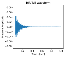
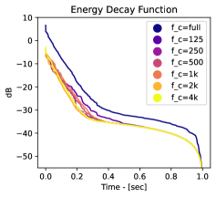
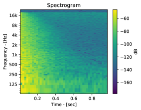
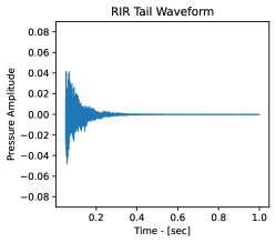
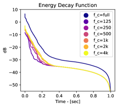
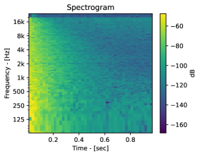
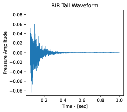
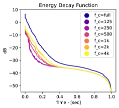
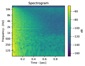
The DECOR model and the FiNS baseline successfully predict the RIR head from the RIR tail, as indicated by the example shown in Figure 5. The models correctly estimate the temporal and spectral characteristics of the tail, and also the sound decay behavior shows good agreement with the ground truth. Table 1 summarizes the evaluation metrics on the test dataset, which contains unseen rooms from the datasets listed in Section 2.3.2. DECOR achieves similar MSTFT and T60 performance as the baseline, but the EDF and DRR errors are higher than those of the baseline.

We conducted an informal perceptual evaluation of our model. Sound examples can be found on the project website. Both models produced RIRs closely matching the timbre of the ground truth room. However, the FiNS baseline model generated unnatural-sounding RIRs, despite achieving lower errors than the DECOR model. The waveform synthesized by the baseline contains sparse, large amplitude peaks, as illustrated on the bottom left of Figure 5. These peaks add an unnatural graininess that is not present in the ground truth RIR tail. In contrast, our predicted RIRs achieve much smoother-sounding RIRs. This is because DECOR predicts parameters for the exponential decay model in Eq. (4), thus generating smoothly decaying RIRs with exponential decay curves.

Figure 4: Damping density per filter $\bm{A}$ for a predicted RIR. The model predicts one dominant decay time per filter, while slightly activating adjacent decay times, and inactivating all other decay times. Note that the dominant decay time is slightly different across filters.

	Pressure Waveform	Energy Decay Function	Spectrogram
Ground truth
DECOR
FiNS

Figure 5: Model outputs on a test dataset sample. The top row is the ground truth; the middle row is the DECOR model, and the bottom row is the FiNS baseline. The left column shows the RIR tail waveform. The middle column shows the unnormalized EDF from the full-length broadband signal (darkest) and in octave bands (dark to light with increasing band center frequency). The right column shows the magnitude spectrogram of the full-length RIR.

3.4 Generalization Power

Lastly, we evaluated DECOR on an unseen measured RIR dataset to investigate its generalization power. We use the BUT ReverbDB [43] dataset, and the corresponding error values are reported in Table 2.

The reported values across all metrics indicate that our model performs worse on unseen datasets than on the test dataset RIRs, which were an unseen subset from the datasets used during training. However, the baseline model also performs significantly worse and has worse T60 and DRR errors than DECOR.

4 Discussion

The results show that DECOR performed successfully on the RIR completion task. It generated a realistic RIR tail with temporal, spectral, and sound energy decay characteristics matching the ground truth. Although our model performs slightly worse than the baseline, it is more than thirty times smaller.

Secondly, the results show that the DECOR model’s performance decreases significantly when evaluating it on an unseen dataset. A similar loss of generalization performance was already noted in the paper on the FiNS baseline method [32]. Additionally, our training dataset was rather small and only contained measured RIRs. Increasing the amount of training data will likely improve the generalization error. However, the selection of datasets will be crucial. The direct and early reflections of future training datasets must be physically accurate for the model to learn meaningfully across datasets. Additionally, synthesized datasets may contain artifacts due to the hybrid simulation approaches utilized, potentially making them unsuitable for training our model.

Our model achieves good results in the context of RIR completion. Extrapolating a signal to twenty times its original length can be considered a challenging task. The difficulty of the task helps to contextualize the network’s performance, for example, when comparing it with results reported in RIR blind estimation performance of the original FiNS model [32], where on their test set, MSTFT error was 1.18 [cf. 1]. The informal perceptual evaluation also supports the idea that our synthesized RIRs sound similar to the ground truth regarding timbre, reverberation time, and DRR.

One possible use case for the RIR completion task is real-time RIR generation for augmented and virtual reality (AR/VR), thus motivating an approach with low computational complexity and storage requirements. Our proposed method DECOR goes one step further where its encoder-decoder essentially performs a regression task to determine the activation of a range of decay rates, see Fig. 4. DECOR predicts the amplitude matrix $\bm{A}$ which is analogous to the discretized ”damping density” termed by Kuttruff [7], and these values can be used as parameters in diverse rendering techniques.

5 Conclusion

In this paper, we propose a deep neural model DECOR that closely approximates an RIR given the short beginning segment. The performance of the DECOR model is slightly worse but comparable to a baseline method, yet is more than thirty times smaller and has fewer noticeable artifacts. DECOR was found to perform worse on an unseen dataset, but it is not surprising given the small training dataset. While the proposed method has much room for improvement and exploration, interpretations of the model’s intermediate stage demonstrate that RIR completion is a solvable task and a promising new direction for the fast generation of room impulse responses.

Declarations

Availability of data and materials

All data used in the training and evaluation of the deep learning models in this paper are from publicly available datasets. DOIs for all datasets are included in the reference list.

Competing interests

The authors declare that they have no competing interests.

Funding

Jackie Lin was funded by the Aalto University School of Electrical Engineering, Funding for multidisciplinary MSc theses.

Authors’ contributions

Jackie Lin conceptualized the publication and implemented the proposed method, ran experiments, produced plots, and wrote the article. Sebastian Schlecht and Georg Götz contributed key ideas, advised the work, and revised the article. All authors reviewed and approved the final manuscript.

Acknowledgements

We would like to thank Ricardo Falcon Perez and Kyungyun Lee for their invaluable input and guidance on designing and running deep learning experiments. We acknowledge the computational resources provided by the Aalto Science-IT project.

References

- \bibcommenthead
- Savioja and Svensson [2015] Savioja, L., Svensson, U.P.: Overview of geometrical room acoustic modeling techniques. J. Acoust. Soc. Am. 138(2), 708–730 (2015) https://doi.org/10.1121/1.4926438
- Allen and Berkley [1979] Allen, J.B., Berkley, D.A.: Image method for efficiently simulating small-room acoustics. J. Acoust. Soc. Am. 65(4), 943–950 (1979) https://doi.org/10.1121/1.382599
- Borish [1984] Borish, J.: Extension of the image model to arbitrary polyhedra. J. Acoust. Soc. Am. 75(6), 1827–1836 (1984) https://doi.org/10.1121/1.390983
- Krokstad et al. [1968] Krokstad, A., Strøm, S., Sørsdal, S.: Calculating the acoustical room response by the use of a ray tracing technique. J. Sound Vib. 8(1), 118–125 (1968) https://doi.org/10.1016/0022-460x(68)90198-3
- Kulowski [1985] Kulowski, A.: Algorithmic representation of the ray tracing technique. Appl. Acoust. 18(6), 449–469 (1985) https://doi.org/10.1016/0003-682X(85)90024-6
- Vorländer [1989] Vorländer, M.: Simulation of the transient and steady-state sound propagation in rooms using a new combined ray-tracing/image-source algorithm. J. Acoust. Soc. Am. 86(1), 172–178 (1989) https://doi.org/10.1121/1.398336
- Kuttruff [2009] Kuttruff, H.: Room Acoustics, Fifth Edition. CRC Press, New York (2009)
- Lewers [1993] Lewers, T.: A combined beam tracing and radiatn exchange computer model of room acoustics. Appl. Acoust. 38(2-4), 161–178 (1993) https://doi.org/10.1016/0003-682X(93)90049-C
- Savioja et al. [1994] Savioja, L., Rinne, T., Takala, T.: Simulation of room acoustics with a 3-D finite difference mesh. In: Proc. Int. Computer Music Conf., Aarhus, Denmark, pp. 463–466 (1994)
- Botteldooren [1995] Botteldooren, D.: Finite-difference time-domain simulation of low-frequency room acoustic problems. J. Acoust. Soc. Am. 98(6), 3302–3308 (1995) https://doi.org/%****␣main.bbl␣Line␣175␣****10.1121/1.413817
- Lehmann and Johansson [2009] Lehmann, E.A., Johansson, A.M.: Diffuse reverberation model for efficient image-source simulation of room impulse responses. IEEE/ACM Trans. Audio, Speech, Language Process. 18(6), 1429–1439 (2009) https://doi.org/10.1109/TASL.2009.2035038
- Kristiansen et al. [1993] Kristiansen, U., Krokstad, A., Follestad, T.: Extending the image method to higher-order reflections. Appl. Acoust. 38(2-4), 195–206 (1993) https://doi.org/10.1016/0003-682X(93)90051-7
- Meng et al. [2002] Meng, Z., Sakagami, K., Morimoto, M., Bi, G., Alex, K.C.: Extending the sound impulse response of room using extrapolation. IEEE Trans. Speech Audio Process. 10(3), 167–172 (2002) https://doi.org/10.1109/TSA.2002.1001981
- Välimäki et al. [2012] Välimäki, V., Parker, J.D., Savioja, L., Smith, J.O., Abel, J.S.: Fifty Years of Artificial Reverberation. IEEE/ACM Trans. Audio, Speech, Language Process. 20(5), 1421–1448 (2012) https://doi.org/10.1109/TASL.2012.2189567
- Välimäki et al. [2016] Välimäki, V., Parker, J., Savioja, L., Smith, J.O., Abel, J.: More than 50 years of artificial reverberation. In: Proc. 60th Int. Audio Eng. Soc. Conf. Dereverb. Reverb. Audio, Music, Speech (DREAMS), Leuven, Belgium (2016)
- Moorer [1979] Moorer, J.A.: About this reverberation business. Computer Music Journal 3(2), 13–28 (1979) https://doi.org/10.2307/3680280
- Jot and Chaigne [1991] Jot, J.-M., Chaigne, A.: Digital delay networks for designing artificial reverberators. In: Proc. 90th Audio Eng. Soc. Conv., Paris, France (1991)
- Jot [1992] Jot, J.-M.: An analysis/synthesis approach to real-time artificial reverberation. In: Proc. IEEE Int. Conf. Acoust. Speech Signal Process. (ICASSP), San Francisco, CA, USA, pp. 221–224 (1992). https://doi.org/10.1109/ICASSP.1992.226080
- Järveläinen and Karjalainen [2007] Järveläinen, H., Karjalainen, M.: Reverberation modeling using velvet noise. In: Proc. 30th Int. Audio Eng. Soc. Conf. Intelligent Audio Env., Saariselkä, Finland (2007)
- Götz et al. [2021] Götz, G., Schlecht, S.J., Pulkki, V.: Motus: A dataset of higher-order Ambisonic room impulse responses and 3D models measured in a room with varying furniture. Zenodo, ??? (2021). https://doi.org/10.5281/zenodo.4923187
- Lee et al. [2023] Lee, S., Choi, H.-S., Lee, K.: Yet another generative model for room impulse response estimation. In: Proc. IEEE Workshop Appl. Signal Process. Audio Acoust. (WASPAA), New Paltz, NY, USA (2023). https://doi.org/10.1109/WASPAA58266.2023.10248189
- Ratnarajah et al. [2022] Ratnarajah, A., Tang, Z., Aralikatti, R., Manocha, D.: Mesh2ir: Neural acoustic impulse response generator for complex 3D scenes. In: Proceedings of the 30th ACM International Conference on Multimedia, pp. 924–933 (2022). https://doi.org/10.1145/3503161.3548253
- Borrel-Jensen et al. [2021] Borrel-Jensen, N., Engsig-Karup, A.P., Jeong, C.-H.: Physics-informed neural networks for one-dimensional sound field predictions with parameterized sources and impedance boundaries. JASA Express Lett. 1(12, paper no. 122402) (2021) https://doi.org/10.1121/10.0009057
- Karakonstantis and Fernandez-Grande [2023] Karakonstantis, X., Fernandez-Grande, E.: Room impulse response reconstruction using physics-constrained neural networks. In: Proc. 10th Conv. European Acoust. Assoc. (Forum Acusticum), Turin, Italy (2023). https://doi.org/10.61782/fa.2023.0804
- Luo et al. [2022] Luo, A., Du, Y., Tarr, M., Tenenbaum, J., Torralba, A., Gan, C.: Learning neural acoustic fields. In: Proc. 36th Conf. Neural Inf. Process. Syst. (NeurIPS), New Orleans, LA, USA, pp. 3165–3177 (2022)
- Richard et al. [2022] Richard, A., Dodds, P., Ithapu, V.K.: Deep impulse responses: Estimating and parameterizing filters with deep networks. In: Proc. IEEE Int. Conf. Acoust. Speech Signal Process. (ICASSP), Singapore, Singapore, pp. 3209–3213 (2022). https://doi.org/10.1109/ICASSP43922.2022.9746135
- Sarroff and Michaels [2020] Sarroff, A., Michaels, R.: Blind arbitrary reverb matching. In: Proc. 23rd Int. Conf. Digital Audio Effects (DAFx), Online Conference, pp. 24–30 (2020)
- Singh et al. [2021] Singh, N., Mentch, J., Ng, J., Beveridge, M., Drori, I.: Image2reverb: Cross-modal reverb impulse response synthesis. In: Proc. IEEE/CVF Int. Conf. Computer Vision (ICCV), Montreal, QC, Canada, pp. 286–295 (2021). https://doi.org/10.1109/ICCV48922.2021.00035
- Kon and Koike [2019] Kon, H., Koike, H.: Estimation of late reverberation characteristics from a single two-dimensional environmental image using convolutional neural networks. J. Audio Eng. Soc. 67(7/8), 540–548 (2019) https://doi.org/10.17743/jaes.2018.0069
- Liang et al. [2023] Liang, S., Huang, C., Tian, Y., Kumar, A., Xu, C.: AV-NeRF: Learning neural fields for real-world audio-visual scene synthesis. arXiv preprint arXiv:2302.02088 (2023) https://doi.org/10.48550/arXiv.2302.02088
- Koo et al. [2021] Koo, J., Paik, S., Lee, K.: Reverb conversion of mixed vocal tracks using an end-to-end convolutional deep neural network. arXiv preprint arXiv:2103.02147 (2021) https://doi.org/10.48550/arXiv.2103.02147
- Steinmetz et al. [2021] Steinmetz, C.J., Ithapu, V.K., Calamia, P.: Filtered noise shaping for time domain room impulse response estimation from reverberant speech. In: Proc. IEEE Workshop Appl. Signal Process. Audio Acoust. (WASPAA), Online conference, pp. 221–225 (2021). https://doi.org/10.1109/WASPAA52581.2021.9632680
- Moore et al. [2013] Moore, A.H., Brookes, M., Naylor, P.A.: Room geometry estimation from a single channel acoustic impulse response. In: Proc. 21st European Signal Process. Conf. (EUSIPCO 2013), Marrakech, Morocco (2013)
- Markovic et al. [2013] Markovic, D., Antonacci, F., Sarti, A., Tubaro, S.: Estimation of room dimensions from a single impulse response. In: Proc. IEEE Workshop Appl. Signal Process. Audio Acoust. (WASPAA), New Paltz, NY, USA (2013). https://doi.org/10.1109/WASPAA.2013.6701867
- Kuster [2008] Kuster, M.: Reliability of estimating the room volume from a single room impulse response. J. Audio Eng. Soc. 124(2), 982–993 (2008) https://doi.org/10.1121/1.2940585
- Yu and Kleijn [2020] Yu, W., Kleijn, W.B.: Room acoustical parameter estimation from room impulse responses using deep neural networks. IEEE/ACM Trans. Audio, Speech, Language Process. 29, 436–447 (2020) https://doi.org/10.1109/TASLP.2020.3043115
- Götz et al. [2022] Götz, G., Falcón Pérez, R., Schlecht, S.J., Pulkki, V.: Neural network for multi-exponential sound energy decay analysis. J. Acoust. Soc. Am. 152(2), 942–953 (2022) https://doi.org/10.1121/10.0013416
- Yamamoto et al. [2020] Yamamoto, R., Song, E., Kim, J.-M.: Parallel WaveGAN: a fast waveform generation model based on generative adversarial networks with multi-resolution spectrogram. In: Proc. IEEE Int. Conf. Acoust. Speech Signal Process. (ICASSP), Online Conference, pp. 6199–6203 (2020). https://doi.org/10.1109/ICASSP40776.2020.9053795
- Prawda et al. [2022] Prawda, K., Schlecht, S.J., Välimäki, V.: Calibrating the Sabine and Eyring formulas. J. Acoust. Soc. Am. 152(2), 1158–1169 (2022) https://doi.org/10.1121/10.0013575
- Klein and Amengual Garí [2023] Klein, F., Amengual Garí, S.V.: The R3VIVAL Dataset: Repository of room responses and 360 videos of a variable acoustics lab. In: Proc. IEEE Int. Conf. Acoust. Speech Signal Process. (ICASSP), Rhodes Island, Greece (2023). https://doi.org/10.1109/ICASSP49357.2023.10097257
- Traer and McDermott [2016] Traer, J., McDermott, J.H.: Statistics of natural reverberation enable perceptual separation of sound and space. Proc. Natl. Acad. Sci. U.S.A. 113(48), 7856–7865 (2016) https://doi.org/10.1073/pnas.1612524113
- Wright and Demeure [2021] Wright, L., Demeure, N.: Ranger21: a synergistic deep learning optimizer. arXiv preprint arXiv:2106.13731 (2021) https://doi.org/10.48550/arXiv.2106.13731
- Szöke et al. [2019] Szöke, I., Skácel, M., Mošner, L., Paliesek, J., Černockỳ, J.: Building and evaluation of a real room impulse response dataset. IEEE J. Sel. Top. Signal Process. 13(4), 863–876 (2019) https://doi.org/10.1109/JSTSP.2019.2917582
- Schroeder [1965] Schroeder, M.R.: New method of measuring reverberation time. J. Acoust. Soc. Am. 37(3), 1187–1188 (1965) https://doi.org/10.1121/1.1909343