Tracking optimal feedback control under uncertain parameters
Abstract.
Optimal control problems of tracking type for a class of linear systems with uncertain parameters in the dynamics are investigated. An affine tracking feedback control input is obtained by considering the minimization of an energy-like functional depending on a finite ensemble of training/sample parameters. It is computed from the nonnegative definite solution of an associated differential Riccati equation. Simulations are presented showing the tracking performance of the computed input for trained as well as untrained parameters.
MSC2020: 34F05, 49J15, 49J20, 49N10, 93B52, 93C15, 93C20
Keywords: Ensemble feedback control, Tracking control, Parameter-dependent systems
1 Johann Radon Institute for Computational and Applied Mathematics, ÖAW, Altenbergerstrasse 69, 4040 Linz, Austria.
2 Institute of Mathematics and Scientific Computing, Karl-Franzens University of Graz, Heinrichstrasse 36, 8010 Graz, Austria, and Johann Radon Institute for Computational and Applied Mathematics, ÖAW, Altenbergerstrasse 69, 4040 Linz, Austria.
Emails: philipp.guth@ricam.oeaw.ac.at, karl.kunisch@uni-graz.at,
sergio.rodrigues@ricam.oeaw.ac.at
1. Introduction
Tracking problems over a finite time-horizon for linear autonomous control systems in the form
are investigated, with state , for time , and . The state space is a separable Hilbert space, is the infinitesimal generator of a semigroup , and is a bounded linear operator. The control space is another separable Hilbert space. The initial condition is given and the choice of the control input is at our disposal.
In many situations the dynamics depends on uncertain or unknown parameters. Thus, we address the design of a robust feedback control operator for parameter-dependent systems of the form
| (1.1) |
with an uncertain/unknown parameter in a given set , for some positive integer . More precisely, we aim at driving the state as close as possible to a given target function . For this purpose, if we knew the exact value of , we could follow a classical strategy by considering the minimization of energy-like functionals as
| (1.2) |
subject to (1.1). In this way we would obtain a feedback control input , with the input feedback operator depending on , arriving at
If we do not know , we could try to use a guess (or an estimate) for it. Applying the feedback corresponding to the guess, we would arrive at
If our estimate is good enough so that is small, then, we can hope that this feedback input will provide good tracking properties.
However, finding a good estimate and subsequently computing the optimal input feedback can be a time consuming task and can be impractical for real time applications. So, we propose to design an input control operator , depending on an a priori fixed finite subset , but independent of a particular realization of .
1.1. Related literature
We could not find works, in the literature, on finite time-horizon (i.e., ) tracking optimal feedback control problems for a general target under uncertainty. Here we propose and analyze a feedback input control operator inspired by the strategy in [11], for the case in the case of infinite time-horizon, .
The strategy in [11] applies classical optimal control theory for linear systems to an auxiliary extended system depending on an ensemble of sample parameters . In the context of tracking objectives we use the optimal control theory developed, for example, in [14] and [23, Ch. 8.3]. As we shall recall later, after a change of variables as , the problem of tracking , under linear dynamics for , is reduced to the problem of tracking , under affine dynamics for , leading us to the theory in [3, Part IV, Ch. 1, Sect. 7.1].
The addressed problem falls into the larger class of optimization under uncertainty, see, for example [1, 10, 16, 20] treating open-loop optimal control problems or stationary optimization problems. The present work focuses on optimal control problems in feedback form.
We underline that the uncertainty enters the system through the operator , thus it does not necessarily enter in an affine manner as . Noise entering the dynamics in an affine manner is for instance investigated in [17, Ch. 3.6] and [8, Ch. III].
Controlled systems with uncertainties entering the system operator arise, for instance, in the case of parabolic equations with uncertain diffusion, reaction, or convection coefficients. Another case is that of damped wave-like equations with uncertain damping coefficients.
In the context of stabilization (i.e., ), examples of research towards feedback controls for parameterized systems include [25], where robustness criteria for linear systems, and error bounds are obtained for the perturbed system and control matrices under which a Riccati based nominal feedback law remains stable. In [12, 15] online-offline strategies are proposed to stabilize a parameter-dependent controlled dynamical system. See also [4], where stabilizability is investigated for an ensemble of Bloch equations, and [21], where a bilinear stabilizing feedback is constructed for an ensemble of oscillators.
In the context of controllability, at/in a given time , , the concept of ensemble controllability (controllability of ensembles of systems; simultaneous controllability), is discussed in [18, 13, 6], [19, Ch. 5], [24, Ch. 11.3]. In [26] the notion of averaged controllabity, is discussed and a Kalman-type rank condition is derived; see also [5].
1.2. Contents and notation
The manuscript is structured as follows. In Section 2.1 we consider an extended system with copies of the dynamics corresponding to the parameters in a finite training ensemble and construct a time-dependent feedback input operator for this extended system in Section 2.2. Then, in Section 2.3 we use to construct a feedback control for the original system. Subsequently, we compare the cost of this later feedback with the optimal one in case we knew the uncertain parameter in Section 3; see Corollary 3.5. Besides, in Section 4 we also compare the corresponding trajectories and control inputs; see Corollary 4.5. Finally, results of numerical experiments are reported in Section 5.
Concerning notation, given real numbers and separable Banach spaces and , the space of continuous functions from into is denoted by and the Bochner space of strongly measurable square integrable functions from the interval into is denoted by and we also denote the subspace . Since the time horizon will be fixed throughout this manuscript, to shorten the exposition, sometimes we shall denote
| (1.3) |
By we denote the space of linear continuous mappings from into , and in case we use the shorter .
2. Feedback controls for tracking objectives
We fix a positive integer and a finite ensemble . Further, we consider a more general version of (1.2) as follows; see [3, Part IV, Ch. 1, Eq. (1.2)]. We fix two more separable Hilbert spaces, and , and two bounded linear operators and . Then, we look for a control input , which minimizes
| (2.1) |
with and each pair subject to (1.1) with .
We can find the minimizing control input in feedback form , , where is affine on the difference , with a translation part depending on the residual of the target when plugged into the uncontrolled system. We aim at a robust feedback , in the sense that by applying for parameters , we should observe the desired tracking property towards . With such a feedback input, for any given fixed , system (1.1) reads
We shall assume that the state space is a pivot space, that is, we will identify it with its continuous dual, . Further, we assume that is isomorphic to a closed subspace of , so that we can consider as a pivot space as well, . These identifications are common and convenient in (optimal) control applications (cf. introductory notation in [24, Ch. 4]).
2.1. Extended system.
For each , it is assumed that is the infinitesimal generator of a -semigroup of bounded linear operators on . The adjoint operator to in is denoted by . Equipping the domain of in with the inner product , , with the topology induced by the graph norm, becomes a Hilbert space, and .
Next, let us consider the Cartesian product with the usual inner product , for and . Further, we define the extension operator as
Its adjoint is given by
Using the ensemble of operators , , we introduce the ensemble operator
| (2.2) |
where . We also define, for a given Hilbert space and an operator ,
Now, we can reformulate the problem of minimizing (2.1) with each subject to (1.1), for all , as:
| minimize | ||||
| (2.3a) | ||||
| subject to | (2.3b) | |||
where and .
We observe that , defined in (2.2), is the infinitesimal generator of the -semigroup
of bounded linear operators on .
2.2. Optimal control input for the extended system.
Based on existing results for Riccati equations, in this section we ensure the existence and uniqueness of a feedback control for problem (2.3).
For this purpose we introduce the cone of bounded, linear, self-adjoint, and nonnegative operators in endowed with the norm of . The Riccati operators will be sought as strongly continuous operator-valued functions in the set , which is endowed with the topology of strong convergence, i.e., if and only if there holds in , see e.g., [3, Part IV, Section 2.1]
For simplicity, we shall transform our problem of tracking to a problem of tracking (subject to an inhomogeneous state equation). In this manner we can more directly profit from existing theory on Riccati equations.
Let the target satisfy . Denoting
| (2.4) |
problem (2.3) becomes the problem
| minimize | ||||
| (2.5a) | ||||
| subject to | (2.5b) | |||
with .
Consider, for time , the operator differential Riccati equation
| (2.6) |
The dynamics equation in (2.6) is understood in the sense that for any the function is differentiable and satisfies for almost all ,
From [3, Thm. 2.1, Part IV, Ch. 1] we know that (2.6) admits a unique solution in . In the following theorem we recall from [3, Thm. 7.1, Part IV, Ch. 1], how to construct the optimal pair of feedback control and corresponding state of (2.5a) subject to (2.5b) (and thus for (2.3a) subject to (2.3b)).
2.3. From the extended system to the original one
By construction of the feedback , we expect that will be small. Consequently, we can expect that the component of the difference to the target will be small for all . By solving the extended system we obtain a tracking control input for all . In our context this input is of auxiliary nature, indeed this auxiliary extended state is not available in practice. Rather the goal of this section is to propose a feedback depending only on the state of the original unknown system.
We define the feedback input operator which is constructed by means of computed for the extended system, by
| (2.11) |
Remark 2.2.
In (2.11), the “definition ” simply means that sometimes, for simplicity of the exposition, we will omit the dependence of on .
Therefore, we arrive at the closed-loop system
| (2.12) |
Defining , we find , hence
| (2.13a) | ||||
| with | ||||
| (2.13b) | ||||
Since the linear part of the affine feedback is strongly continuous, that is, for each , and the translation term is in , the above closed-loop system (2.13) has a unique solution for each , (see, e.g., [3, Prop. 3.4, Part II, Ch. 1]). Consequently, there is a unique solution for system (2.12), for any given .
Finally, note that the feedback can also be applied if the true parameter is not a member of the training set , provided that (cf., (2.4)). This will be the generic case in the following sections.
2.4. Order of sequence of training parameters
By construction the matrix , defining the free dynamics of the extended auxiliary system as in (2.3b), depends on the order of the training parameters in the sequence . In spite of this fact, we show that the resulting feedback input as in (2.11), for the original system, is independent of that order. In this sense, we can speak about set of training parameters, instead of sequence of training parameters. Indeed, let be a permutation matrix , and let be the permutation constructed as follows: the entries of are replaced by the identity operator in and the entries are replaced by the zero operator in .
As an example, in case ,
Identifying the sequence with a column vector in , we permute the parameters as . For the permuted/reordered vector, the extended matrix will read
where . Recall that, since and are permutations we have and . By (2.6) we find that solves
Now, observe that , which gives us the analogue of (2.6)
Therefore is the solution of the Riccati equation for the permuted sequence of parameters. Consequently, the feedback input in (2.11) will read, since we also have
where satisfies the analogue of (2.9),
| (2.14) |
with the analogue of in (2.4),
Thus, to show that , it is enough to show that .
By (2.14), using and ,
| (2.15) |
3. Optimal controls and costs
In this section we investigate the cost associated with the feedback (2.11) and compare it to the optimal cost associated with the input (2.7) for the extended system . Further, we consider a comparison with the optimal cost for system , corresponding to the case that the true parameter is known. For such comparisons, we shall make additional assumptions on the family of operators .
We will assume that we have another separable Hilbert space that is continuously and densely embedded in , which leads to the Gelfand triplet . We also assume to be given a family of continuous bilinear forms , parametrized by , each form being – coercive, more precisely,
| (3.1) |
We associate with the operator defined as
| (3.2) | ||||
The operators are closed and densely defined in and can be uniquely extended to operators . For each , generates an analytic semigroup on , which is exponentially bounded (i.e., ).
The following assumption will be made throughout the remainder of the paper.
Assumption 3.1.
By Assumption 3.1, we can introduce the common domain
| (3.3) |
In particular is independent of the ensemble .
Now, recalling the short notation in (1.3), it is known (see, e.g., [3, Thm. 1.1, Part II, Ch. 2]) that for and there is a unique solution of . From (as assumed in Sect. 2.2) we find
| (3.4) |
Recall that (from, e.g., [3, Thm. 1.1, Part II, Ch. 2]), we have that
| (3.5a) | |||
| is an isomorphism. Hence, there exists a constant such that | |||
| (3.5b) | |||
3.1. Comparing optimal costs
Let us fix and consider the problem:
| minimize | (3.6a) | |||
| subject to | (3.6b) | |||
In the following we will use the notation to denote the operator defined as in (2.2) with the same parameter in each component.
Lemma 3.2.
Proof.
Given , the optimality conditions for (2.5), with , are
| (3.8a) | |||||
| (3.8b) | |||||
| (3.8c) | |||||
and for (3.6), they are
The reader is reminded that the factor , in (3.8b), accounts for taking the sum over the ensemble ; see (2.5a).
Defining
we obtain
| (3.9a) | |||||
| (3.9b) | |||||
| (3.9c) | |||||
Moreover, we have and , and due to , we obtain , and thus (cf. [3, Thm. 1.4, Part II, Ch. 2]).
Hence, we find the identity
| (3.10) | ||||
| and, using , we also have | ||||
| (3.11) | ||||
Subtracting (3.10) from (3.11), and using (3.9c), lead us to
| (3.12) | ||||
| (3.13) |
Next, we use a duality argument to estimate the norm of . Let us denote by the unit ball in a given Hilbert space . Let be arbitrary and let be the solution of
for time . Then, we have
where we used (3.9b). Since (see, e.g., [7, Thm. 1, Ch. XVIII]), we have , for some constant . By noticing that and recalling the isomorphism in (3.5), we obtain
| (3.14) |
where is as in (3.5) and with .
Next, we compare the value of the optimal costs associated with the ensemble optimal control problem (2.5) and the single parameter optimal control problem (3.6).
Corollary 3.3.
3.2. Cost of the proposed performant feedback control
We compare the minimal cost associated with the minimizer of the extended system problem (2.5) to the cost associated with the solution of (2.12) resulting from the feedback control given in (2.11).
The following result quantifies the difference of this feedback control associated to the single unknown parameter compared to the optimal control associated to the ensemble of training parameters in the sense of the associated costs.
Theorem 3.4.
Assume that , let be the minimizer of (2.5) with . Further, let and let be the solution of
| (3.18) |
and let . Then, there holds
| (3.19) |
Proof.
We commence by commenting on the regularity of and which will be used throughout the proof. Due to (3.3), we have that , for all (see, e.g., [3, p. 183]). Consequently, it follows by maximal regularity theory that ; see (1.3) and [3, p. 187]. Further, since , we have as well.
Next, recalling (2.10), the minimal cost is given by
| (3.20) |
We observe that
| (3.21) |
and, denoting , we find
| (3.22a) | ||||
| (3.22b) | ||||
| (3.22c) | ||||
| (3.22d) | ||||
Using , where we have abbreviated
| (3.23) |
we obtain
| (3.24a) | |||
| (3.24b) | |||
| (3.24c) | |||
Hence, with , we use
to obtain
Recalling system (2.9), satisfied by , we find
| (3.26a) | ||||
| with | (3.26b) | |||
3.3. Remarks
Within the statement on Corollary 3.5 we use two operator norms for the difference , namely, and . We may wonder whether these norms are equivalent in the intersection space . We can provide a condition which ensures equivalence as follows.
Let be as in Corollary 3.5 and assume that commutes which each operator with index in the training set . Define , with as in (3.1). This operator generates an analytic semigroup satisfying , thus is an operator of type for some and , and the fractional power can be expressed as contour integral in the resolvent set of ; see [3, p. 167]. From here it follows that commutes with every with .
As a second preliminary for the following computation we recall that since the mapping is an isomorphism between and as well as between and . Thus, there exist constants such that
For and we have
which implies that .
On the other hand, for , there holds
which gives . Hence, for , we find
4. Comparing state trajectories
We compare the state trajectories associated to problems (2.5) and (3.6) and to the system (3.18) under the proposed feedback (2.11).
4.1. Trajectories associated to (2.5) and (3.18)
We have the following result.
Theorem 4.1.
Proof.
With as in (1.3), we have , due to . Denoting , , and , there holds
for and . Using (2.7) and (2.11), we obtain
| (4.2) |
Thus, recalling (3.4) and (3.23), we have that , and we obtain
We can represent the solution (see, e.g., [3, Prop. 3.4, Part II, Ch. 1]) as
leading to the estimate
where we took and used . Multiplication by gives
Then, Gronwall’s lemma gives
and finally we obtain
where we used the Cauchy–Schwarz inequality in the second step. ∎
A close inspection of (4.2) reveals the following bound on the difference of the controls.
4.2. Trajectories associated to (2.5) and (3.6)
We have the following result.
Theorem 4.3.
Proof.
A similar estimate holds for the difference of the corresponding controls, as follows.
Corollary 4.4.
4.3. Trajectories associated to (3.18) and (3.6)
5. Numerical experiments
We present numerical experiments supporting our theoretical findings discussed in Section 3. Moreover, for a given target state , and given a parameter ensemble the performance of the feedback , as defined in (2.11), is compared with the optimal feedback for the ensemble average of the parameters, that is we compare the closed-loop systems
| (5.1) |
for test parameters , and for , in given by
| (5.2) | ||||
| (5.3) |
where solves , with , and solves , , with (cf. Section 2.2; note also that ).
5.1. Oscillator
Let us consider the differential equation
| (5.4) | ||||
| (5.5) |
Thus, the damping parameter is allowed to be uncertain. We consider an ensemble of possible values of , and write the second order equation (5.4), for each , as
| (5.6) | ||||
with , , initial condition , and corresponding states . The target function , is chosen to solve (5.6) with and initial condition . Further, we set , , and , where denotes the identity matrix in .
The parameter ensembles will be described as
where denotes the cardinality of the ensemble, i.e., the number of parameters , , and determines the range of the parameter set, and hence resembles the level of uncertaintiy in the problem. The feedback in (5.3) is not affected by changes in or , since .
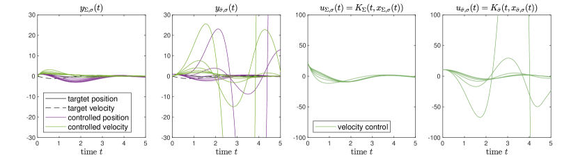
In Figure 1 the feedback control (5.2) is compared to the feedback control (5.3) along with the corresponding closed-loop state trajectories and , respectively. Here, the feedbacks (5.2) and (5.3) are constructed based on the training ensemble , and then tested in the systems with parameters , i.e., test trajectories for each component (position and velocity) are displayed. It is observed that the feedback control (5.2) is much more robust with respect to parameter variations than (5.3): the feedback (5.3) leads to worthless controls, which fail to track the target for the two most unstable test parameters and , whereas the feedback (5.2) still steers the respective states close to the target.
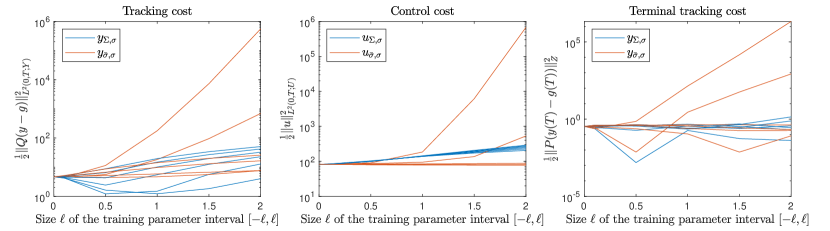
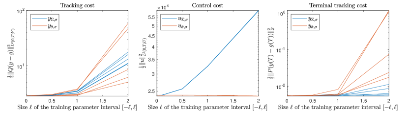
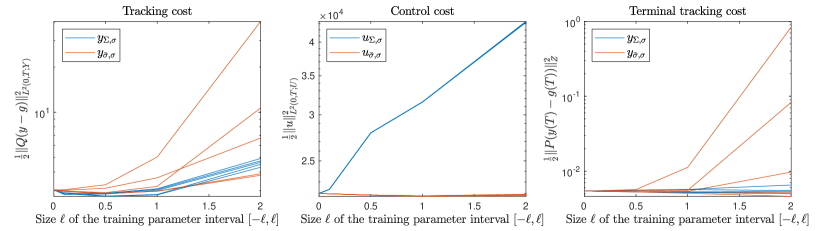
The superior robustness against parameter variations of (5.2) compared to (5.3) is also reflected in the associated costs, which are displayed for different levels of uncertainty in Figure 2. Here, the feedbacks (5.2) and (5.3) are constructed based on the training ensembles , and then tested in the systems with parameters . It is observed that, with increasing level of uncertainty , the feedback (5.3) leads to rapidly increasing tracking cost for the two most unstable test parameters and , whereas the tracking cost associated with (5.2) grows much slower. For , the largest tracking costs in the parameter test set are and , and the terminal tracking costs are and .
For less extreme test parameters, which result in more stable systems, the tracking performance of both feedbacks is similar, while the robust feedback in this case comes at higher control cost, see Figure 2. However, for the two most unstable test parameters and , the feedback (5.2) also leads to smaller control cost than the feedback (5.3).
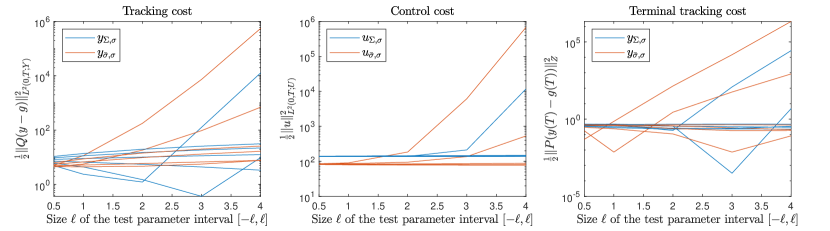
In Figure 3, the feedbacks (5.2) and (5.3) are compared for a fixed training parameter interval and increasing test parameter interval for . A similar relationship is observed: for larger levels of uncertainty , the cost associated with the feedback (5.3) (in red) is much larger for unstable systems than the cost associated with the feedback (5.2) (in blue). For stable systems, the tracking performance of the both feedbacks is again similar. Overall, for this example the robustness of the feedback (5.2) comes at the possible expense of higher control cost.
5.2. Convection-diffusion-reaction equation
Let us consider the parameterized convection-diffusion-reaction equation under Neumann boundary conditions as follows
where , with boundary and the functions represent the support of the actuators, which are modelled as the characteristic functions related to open sets for . It is assumed that the reaction coefficient and the convection coefficient are given constants, and that the parameter enters the diffusion, that is
| (5.7) |
for and for all . Assuming that , it follows that there exist and depending on such that
The representation (5.7) is called a lognormal parameterization, if the parameters are independently and identically distributed (i.i.d.) standard normal random variables, that is , see, e.g., [2]. Parameterizations of this form have origins in Karhunen–Loève expansions of lognormal random fields, see, e.g., [22].
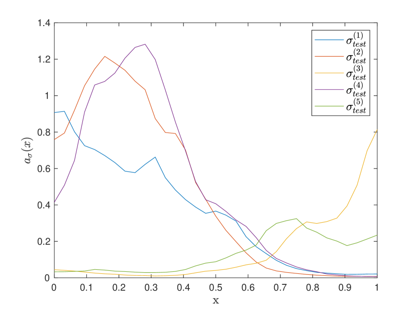
In the numerical experiments actuators are used as , , and . In (5.7) the mean field is set to and it is assumed that the diffusion depends on realizations of i.i.d. standard normal random variables, and parametric basis functions and with , cf. [9]. Further, a constant reaction coefficient is assumed, and we set , where is the orthogonal projection in onto , where , and in (2.1), where denotes the identity operator in , as well as the initial condition . The target solves the heat equation with the same boundary and initial data.
To construct the feedbacks, training vectors, each containing realizations of i.i.d. standard normal random variables, are drawn. In order to investigate different variance levels in Figures 5 and 7, the training vectors are multiplied by a scalar . The feedbacks are then tested with different test parameters, each of which consists of realizations of i.i.d. standard normal random variables.
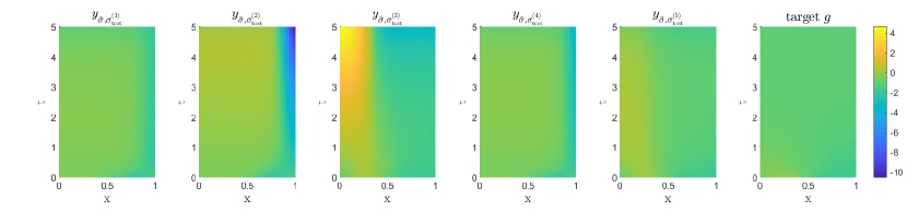
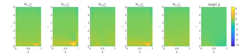
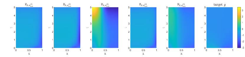
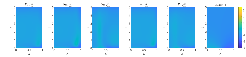
Results without convection are displayed in Figure 5 and Figure 6, and results with convection are displayed in Figure 7 and Figure 8. In the case without convection the feedback (5.2) (in blue) has smaller terminal tracking costs than the feedback (5.3) (in red) for all tested diffusion coefficients, see Figure 5. In addition, it has smaller tracking cost for some of the tested diffusion coefficients. The more robust tracking performance comes at the expense of higher control cost for (5.2).
Similarly, in the case with convection , the feedback (5.2) tracks the target better than the feedback (5.3): while (5.3) clearly fails to track the target for , , and , the feedback (5.2) tracks the target much better for the tested realizations of the diffusion coefficient (5.7), see Figure 8. The improved tracking performance of (5.2) is reflected in the associated costs in Figure 7 and again comes at the expense of higher control cost. The control costs are insensitive to changes of the test parameters, such that no difference between the cost for different test parameters can be seen in Figure 7. The same phenomenon is observed in Figure 5.
In summary, in both cases the feedback (5.2) is more robust against variations in the diffusion coefficient at the cost of higher control costs.
Finally, in accordance with Corollary 3.5, the costs converge as the difference of the test parameters tend to zero, i.e., as tends to , see Figures 5 and 7.
Aknowlegments. S. Rodrigues gratefully acknowledges partial support from the State of Upper Austria and Austrian Science Fund (FWF): P 33432-NBL.
References
- [1] B. Azmi, L. Herrmann, and K. Kunisch. Analysis of RHC for stabilization of nonautonomous parabolic equations under uncertainty. SIAM J. Control Optim., 62(1):220–242, 2024. doi:10.1137/23M1550876.
- [2] I. Babuška, F. Nobile, and R. Tempone. A stochastic collocation method for elliptic partial differential equations with random input data. SIAM J. Numer. Anal., 45(3):1005–1034, 2007. doi:10.1137/050645142.
- [3] A. Bensoussan, G. Da Prato, M. C. Delfour, and S. K. Mitter. Representation and control of infinite dimensional systems, volume 2. Springer, 2007. doi:10.1007/978-0-8176-4581-6.
- [4] F. C. Chittaro and J.-P. Gauthier. Asymptotic ensemble stabilizability of the Bloch equation. Systems Control Lett., 113:36–44, 2018. doi:10.1016/j.sysconle.2018.01.008.
- [5] J. Coulson, B. Gharesifard, and A.-R. Mansouri. On average controllability of random heat equations with arbitrarily distributed diffusivity. Automatica, 103:46–52, 2019. doi:10.1016/j.automatica.2019.01.014.
- [6] B. Danhane, J. Lohéac, and M. Jungers. Conditions for uniform ensemble output controllability, and obstruction to uniform ensemble controllability. Math. Control. Relat. Fields, 2023. doi:10.3934/mcrf.2023036.
- [7] R. Dautray and J.-L. Lions. Mathematical Analysis and Numerical Methods for Science and Technology, volume 5. Springer, 2000. doi:10.1007/978-3-642-58090-1.
- [8] W. H. Fleming and H. M. Soner. Controlled Markov Processes and viscosity solutions. Springer New York, 2006. doi:10.1007/0-387-31071-1.
- [9] R. N. Gantner. Dimension truncation in QMC for affine-parametric operator equations. In Art B. Owen and Peter W. Glynn, editors, Monte Carlo and Quasi-Monte Carlo Methods, volume 241, pages 249–264. Springer, Cham, 2018. doi:10.1007/978-3-319-91436-7\_13.
- [10] P. A. Guth, V. Kaarnioja, F. Y. Kuo, C. Schillings, and I. H. Sloan. Parabolic PDE-constrained optimal control under uncertainty with entropic risk measure using quasi-Monte Carlo integration. preprint: arXiv:2208.02767 [math.NA], 2022. doi:10.48550/arXiv.2208.02767.
- [11] P. A. Guth, K. Kunisch, and S. S. Rodrigues. Ensemble feedback stabilization of linear systems. preprint: arXiv:2306.01079 [math.OC], 2023. doi:10.48550/arXiv.2306.01079.
- [12] P. A. Guth, K. Kunisch, and S. S. Rodrigues. Stabilization of uncertain linear dynamics: an offline-online strategy. preprint: arXiv:2307.14090 [math.OC], 2023. doi:10.48550/arXiv.2307.14090.
- [13] U. Helmke and M. Schönlein. Uniform ensemble controllability for one-parameter families of time-invariant linear systems. Systems Control Lett., 71:69–77, 2014. doi:10.1016/j.sysconle.2014.05.015.
- [14] M. Hinze. Optimal and instantaneous control of the instationary Navier-Stokes equations. TU Berlin, 2000. Habilitation. URL: https://www.math.uni-hamburg.de/home/hinze/Psfiles/habil_mod.pdf.
- [15] B. Kramer, B. Peherstorfer, and K. Willcox. Feedback control for systems with uncertain parameters using online-adaptive reduced models. SIAM J. Appl. Dyn. Syst., 16(3):1563–1586, 2017. doi:10.1137/16M1088958.
- [16] A. Kunoth and Ch. Schwab. Analytic regularity and GPC approximation for control problems constrained by linear parametric elliptic and parabolic PDEs. SIAM J. Control Optim., 51(3):2442–2471, 2013. doi:10.1137/110847597.
- [17] H. Kwakernaak and R. Sivan. Linear optimal control systems, volume 1072. Wiley-interscience New York, 1969. URL: https://books.google.at/books?id=mf0pAQAAMAAJ.
- [18] M. Lazar and J. Lohéac. Chapter 8 - control of parameter dependent systems. In Emmanuel Trélat and Enrique Zuazua, editors, Numerical Control: Part A, volume 23 of Handbook of Numerical Analysis, pages 265–306. Elsevier, 2022. doi:10.1016/bs.hna.2021.12.008.
- [19] J. L. Lions. Contrôlabilité exacte, perturbations et stabilisation de systèmes distribués: Tome 1, Contrôlabilité exacte. Masson, 1988. URL: https://books.google.at/books?id=NE_vAAAAMAAJ.
- [20] J. Martínez-Frutos, M. Kessler, A. Münch, and F. Periago. Robust optimal Robin boundary control for the transient heat equation with random input data. Internat. J. Numer. Methods Engrg., 108(2):116–135, 2016. doi:10.1002/nme.5210.
- [21] E. P. Ryan. On simultaneous stabilization by feedback of finitely many oscillators. IEEE Trans. Autom. Control, 60(4):1110–1114, 2014. doi:10.1109/TAC.2014.2341893.
- [22] Ch. Schwab and C. J. Gittelson. Sparse tensor discretizations of high-dimensional parametric and stochastic PDEs. Acta Numer., 20:291–467, 2011. doi:10.1017/S0962492911000055.
- [23] E. D. Sontag. Mathematical control theory: deterministic finite dimensional systems. Number 6 in Texts in Applied Mathematics. Springer Science & Business Media, 2 edition, 1998. URL: http://www.sontaglab.org/FTPDIR/sontag_mathematical_control_theory_springer98.pdf.
- [24] M. Tucsnak and G. Weiss. Observation and control for operator semigroups. Springer Science & Business Media, 2009. doi:10.1007/978-3-7643-8994-9.
- [25] R. K. Yedavalli. Robust control of uncertain dynamic systems. Springer, 2014. doi:10.1007/978-1-4614-9132-3.
- [26] E. Zuazua. Averaged control. Automatica, 50(12):3077–3087, 2014. doi:10.1016/j.automatica.2014.10.054.