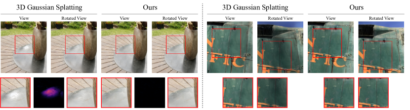
Figure 1. 3D Gaussian Splatting (Kerbl et al., 2023) suffers from popping artifacts during view rotation due to its approximate, global sorting scheme. Our method is able to effectively circumvent short-range popping artifacts (left) and long-range view-inconsistencies (right) during rotation with a novel, hierarchical per-pixel sorting strategy.

This is the teaser figure for the article.

StopThePop: Sorted Gaussian Splatting for View-Consistent Real-time Rendering

Abstract.

Gaussian Splatting has emerged as a prominent model for constructing 3D representations from images across diverse domains. However, the efficiency of the 3D Gaussian Splatting rendering pipeline relies on several simplifications. Notably, reducing Gaussian to 2D splats with a single view-space depth introduces popping and blending artifacts during view rotation. Addressing this issue requires accurate per-pixel depth computation, yet a full per-pixel sort proves excessively costly compared to a global sort operation. In this paper, we present a novel hierarchical rasterization approach that systematically resorts and culls splats with minimal processing overhead. Our software rasterizer effectively eliminates popping artifacts and view inconsistencies, as demonstrated through both quantitative and qualitative measurements. Simultaneously, our method mitigates the potential for cheating view-dependent effects with popping, ensuring a more authentic representation. Despite the elimination of cheating, our approach achieves comparable quantitative results for test images, while increasing the consistency for novel view synthesis in motion. Due to its design, our hierarchical approach is only $4\%$ slower on average than the original Gaussian Splatting. Notably, enforcing consistency enables a reduction in the number of Gaussians by approximately half with nearly identical quality and view-consistency. Consequently, rendering performance is nearly doubled, making our approach 1.6x faster than the original Gaussian Splatting, with a 50% reduction in memory requirements.

1. Introduction

(a)

(b)

(c)

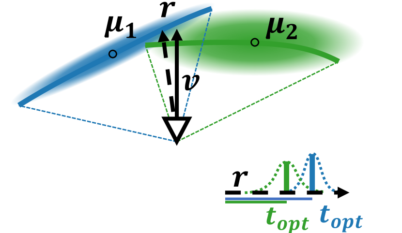
(d)

Figure 2. Effect of collapsing 3D Gaussians into 2D splats and 3DGS’s depth simplification: (a) Integrating Gaussians along view rays $\mathbf{r}$ requires careful consideration of potentially overlapping 1D Gaussians. (b) Using flattened 2D splats and view-space $z$ as depth (projection of $\mathbf{\mu}$ onto $\mathbf{v}$) puts 2D splats on spherical segments around the camera, inverting the relative positions of the two Gaussians along the example view ray. (c) Camera rotation inverts the order along $\mathbf{r}$, resulting in popping. (d) Camera translation does not alter the distance compared to (b).

In recent years, Neural Radiance Fields (NeRFs) (Mildenhall et al., 2020) have triggered a new surge of research around differentiable rendering of 3D representations. Leveraging the traditional volume rendering equation, NeRFs are fully differentiable, enabling continuous optimization to align the representation to diverse input views and support high-quality novel view synthesis. This differentiability also proves valuable in addressing other rendering challenges that necessitate gradient flow and optimization.

Various strategies have arisen to tackle challenges in NeRFs, particularly mitigating the computational costs linked to multilayer perceptron (MLP) evaluation. These approaches include adopting direct voxel representations (Fridovich-Keil et al., 2022), employing feature hash maps (Müller et al., 2022), and exploring tensor factorizations (Chen et al., 2022; Tang et al., 2022)—departing to some extent from the original pure MLP design. A recent notable development in this trajectory is 3D Gaussian Splatting (3DGS) (Kerbl et al., 2023), which renders oriented 3D Gaussians with spherical harmonics (SH) as a view-dependent color representation.

Remaining faithful to the traditional volume rendering equation, 3DGS facilitates gradient flows from image errors to the Gaussians’ positions, shapes, densities, and colors. With an initialization based on structure-from-motion (Snavely et al., 2006), a real-time compute-mode rasterizer, and heuristic-driven densification and sparsification, 3DGS converges to a high-quality representation with compact memory requirements. Consequently, 3DGS has firmly established itself as one of the most widely used methods for 3D scene reconstruction and differentiable rendering.

Colored, semi-transparent 3D Gaussians serve as a versatile representation, but their accurate rendering is challenging. Although the projection of a 3D Gaussian onto a view ray is straightforward, leveraging synergies between neighboring rays under perspective projection proves intricate. Hence, 3DGS approximates them as flattened 2D splats (Zwicker et al., 2002), necessitating depth-based sorting for rendering. 3DGS further simplifies this step by sorting based on the view-space $z$-coordinate of each Gaussian’s mean, effectively projecting splats onto spherical shells reminiscent of Broxton et al. (2020). While this global sorting eases the rendering algorithm, it introduces popping artifacts, i.e., sudden color changes for consistent geometry, during camera rotations due to changes in the relative depth of shells (see Fig. 2).

Fully evaluating all Gaussians in 3D along each view ray while considering their overlap would be ideal, but likely not feasible in real-time. The next best solution involves approximating the location where each Gaussian contributes the most for each view ray, i.e., determining its depth, followed by a correct per-pixel blending. Sorting must now happen for each view ray, rather than globally for all Gaussians; an obvious challenge as it is not uncommon to see thousands of Gaussians be considered for individual rays in 3DGS. To solve this challenge, we propose a novel 3D Gaussian Splatting rendering pipeline that exploits coherence among neighboring view rays on multiple hierarchy levels, interleaving culling, depth evaluation and resorting. We make the following contributions:

• A novel hierarchical 3D Gaussian Splatting renderer that leads to per-pixel sorting of Gaussian splats for both the forward and backward pass of the 3DGS rendering pipeline and thus removes popping artifacts.

• An in-depth analysis of culling and depth approximation strategies, as well as pipeline optimizations and workload distribution schemes for our compute-mode 3DGS hierarchical renderer.

• A discussion and evaluation of various sorting strategies of Gaussian splats and their influence on overall rendering quality and view-consistency.

• An effective automatic method to detect popping artifacts in videos captured from trained 3D Gaussians as well as a user study confirming the results of the presented method.

Our results indicate that a full per-pixel sorted renderer for Gaussian splats eliminates all popping artifacts but reduces rendering speed by $100\times$. Our hierarchical renderer is virtually indistinguishable from a full per-pixel sorted renderer, but only adds an overhead of $4\%$ compared to the original 3DGS.

2. Preliminaries and Related Work

In the following, we review the renderer used in 3DGS. For a complete description of the approach, cf. Kerbl et al. (2023).

2.1. 3D Gaussian Splatting

NeRF-style rendering and 3DGS use the volume rendering equation:

(1) $$C(\mathbf{r})=\int_{0}^{t}c\left(\mathbf{r},t\right)\,\sigma\left(\mathbf{r},t\right)\,T(\mathbf{r},t)\,dt\text{, \hskip 5.0ptwhere}$$

$$T(\mathbf{r},t)=e^{-\int_{0}^{t}\sigma\left(\mathbf{r},s\right)\,ds},$$

$C(\mathbf{r})$ is the output color for a given ray $\mathbf{r}$, $\sigma\left(\mathbf{r},t\right)$ is the opacity along the ray and $c\left(\mathbf{r},t\right)$ is the emitted radiance. 3DGS represents a scene as a mixture of $N$ 3D Gaussians each given by:

$$G_{i}(\mathbf{x})=e^{-\frac{1}{2}(\mathbf{x}-\mathbf{\mu_{i}})^{T}\Sigma_{i}^{-1}(\mathbf{x}-\mathbf{\mu_{i}})}\text{, \hskip 5.0ptwhere}$$

$$\Sigma_{i}=R_{i}S_{i}S_{i}^{T}R_{i}^{T},$$

$\mathbf{\mu}_{i}$ is the Gaussian’s location, $R_{i}$ is a rotation matrix and $S_{i}$ is a scaling matrix, allowing to position, rotate and non-uniformly scale Gaussians in 3D space. When evaluating a 3D Gaussian along a ray, the resulting projection is a 1D Gaussian. It seems natural to evaluate Eqn. (1) considering how multiple Gaussians influence any location along the ray. As there is no elementary indefinite integral known for Gaussians, numerical integration is likely the only option. In practice, this would require a strict sorting of all starting and end points of all Gaussians and sampled numerical integration.

3DGS makes multiple simplifications. First, they consider all Gaussians to be separated in space, i.e., compress their extent to a Dirac delta along the ray. Second, the Dirac delta is located at

(2) $$t_{i}=\mathbf{\mu}_{i}^{T}\mathbf{v},$$

i.e., the projection of the mean $\mathbf{\mu}_{i}$ onto the view direction $\mathbf{v}$, independent of the individual ray $\mathbf{r}$. Third, they approximate the projection of the Gaussian onto all rays, relying on an orthogonal projection approximation considering the first derivative of the 3D Gaussian to construct a 2D splat $G_{2}$ (Zwicker et al., 2002).

These approximations enable faster rendering: Eqn. (1) becomes

(3) $$C(\mathbf{r})=\sum_{i=1}^{N_{\mathbf{r}}}c_{i}\alpha_{i}\prod_{j=1}^{i-1}(1-\alpha_{j}),$$

where $i$ iterates over the $N_{\mathbf{r}}$ Gaussians that influence the ray in the ordering of $t_{i}$, and $\alpha_{i}$ is the opacity of the Gaussian along the ray, i.e., $G_{2}(x,y)$, multiplied by a learned per-Gaussian opacity value.

Because $t_{i}$ is independent of $\mathbf{r}$, a global sort of all $t$ is possible. Naïvely, this would lead to $N_{\mathbf{r}}=N$ for all rays. To reduce the number of Gaussians considered per ray, 3DGS runs a combined depth and tile sorting pre-pass, before evaluating Eqn. (3). For each $16\times 16$ pixel tile and each Gaussian that may potentially contribute to any pixel in this tile—considering the 2D bounding box around the $1\%$ Gaussian contribution threshold—a sorting key is generated with the tile index in the higher order bits and the depth in the lower bits. Sorting those combined keys leads to a $t_{i}$-sorted list for each tile.

2.2. Radiance Field Methods

Contrary to 3DGS, NeRFs (Mildenhall et al., 2020) require sampling a continuous, implicit neural scene representation densely. Therefore, real-time rendering as well as handling unbounded scenes proves difficult. Many follow-up works investigated NeRF extensions to handle unbounded scenes (Barron et al., 2021, 2022, 2023) as well as faster rendering (Müller et al., 2022; Fridovich-Keil et al., 2022; Chen et al., 2022), 3D scene editing (Nguyen-Phuoc et al., 2022; Kuang et al., 2023; Jambon et al., 2023), avatar generation (Zielonka et al., 2023), scene dynamics (Pumarola et al., 2020; Park et al., 2021) and 3D mesh generation (Jain et al., 2022; Poole et al., 2022; Raj et al., 2023).

2.3. 3DGS Follow-up Work

Following the code release and subsequent publication of 3DGS, several extensions have popped up investigating various paradigms, including the editing of trained Gaussians (Chen et al., 2023; Fang et al., 2023), text-to-3D (Tang et al., 2023; Yi et al., 2023) and 4D novel view synthesis (Luiten et al., 2024; Wu et al., 2023). Mip-Splatting (Yu et al., 2023) proposes a 3D smoothing filter and 2D Mip filter to remedy aliasing in 3DGS. Besides them, most approaches merely leverage Gaussians as graphics primitives, whereas our approach tackles current problems with 3DGS.

2.4. Software Rasterization

Our compute-mode rendering pipeline for 3DGS is related to other software-based rendering pipelines. Early works like Pomegranate (Eldridge et al., 2000) and the Larrabee project (Seiler et al., 2008) showed that software pipelines on custom hardware are viable for rendering. Special compute-mode rendering pipelines have been proposed for REYES (Zhou et al., 2009; Tzeng et al., 2010), triangle rasterization (Liu et al., 2010; Laine and Karras, 2011; Patney et al., 2015; Kenzel et al., 2018; Karis et al., 2021) and point clouds (Schütz et al., 2021). Similarly to these efforts, we show that taking into account the specifics of the rendering problem, a compute-mode renderer for sorted Gaussian splats can execute in real-time on modern GPUs.

3. Real-time Sorted Gaussian Splatting

We present a novel per-pixel sorted 3D Gaussian splatting approach, departing from the current global sorting paradigm. Utilizing fast per-pixel depth calculations and a hierarchical intra-tile cooperative sorting approach, our method enhances the accuracy of the resulting sort order. To streamline computations, we incorporate per-tile opacity culling and a fast and GPU-friendly load balancing scheme.

3.1. Global Sorting

3DGS (Kerbl et al., 2023) performs a global sort based on the view-space $z$-coordinate of each Gaussian’s mean $\mu$, see Eqn. (2). This leads to a consistent sort order during translation, but not during rotation, as illustrated in Fig. 2. While 3DGS may use this fact during training to introduce differences between views (and thus reduce the loss), it is in general undesirable, as camera rotations can lead to popping artifacts, which are particularly disturbing when inspecting the optimized 3D scene. Our objective is to stabilize color computations under rotation by splatting Gaussians based on the point of highest contribution along each view ray. Note that, although we improve rendering consistency, we still approximate true 3D Gaussians, neglecting any overlap between them.

0.49 0.49

Figure 3. Our approach to compute $t_{opt}$ places splats along the maximum point of contribution along the view ray $\mathbf{r}$, creating sort orders independent of camera rotation (red view vector) and thus avoiding popping. Note that the shape of $t_{opt}$ is a curved surface and changes with $\mathbf{o}$; cf. Fig. 2.

3.2. Per-pixel Depth and Naïve Sorting

When replacing a 1D Gaussian along the view ray with a Dirac impulse, the mean/maximum of this 1D Gaussian is arguably the best discrete blend location. This maximum, $t_{opt}$, can be computed from the derivative of the 3D Gaussian along the view ray $\mathbf{r}(t)=\mathbf{o}+t\mathbf{d}$:

(4) $$t_{opt} =\frac{\mathbf{d}^{T}\Sigma^{-1}(\mathbf{\mu}-\mathbf{o})}{\mathbf{d}^{T}\Sigma^{-1}\mathbf{d}}.$$

Please see the supplemental material for the step-by-step derivation.

Consider a simple 2D case with an isotropic Gaussian $\Sigma^{-1}=\mathbf{I}$, the camera at $(0,0)$ and the Gaussian at $\mathbf{\mu}=(0,\mu_{y})$. It is easy to see that the depth function follows a cosine as $\mathbf{d}$ is normalized:

$$t=\frac{\mathbf{d}^{T}\mathbf{I}\mathbf{\mu}}{\mathbf{d}^{T}\mathbf{I}\mathbf{d}}=d_{y}\cdot\mu_{y}=\cos(\theta)\mu_{y},$$

where $\theta$ is the angle of the view ray. Thus, we conclude that there is no simple primitive, like, e.g., a plane to represent the $t_{opt}$ which could be rasterized traditionally, see Fig. 3. Therefore, we compute $t_{opt}$ on a per-ray basis.

When reconstructing surfaces, Gaussians often turn very flat, as such, $\Sigma^{-1}$ may become large and lead to instabilities in the computation. Bounding the entries of $S^{-1}$ to $10^{3}$ removes those instabilities in our experiments, by effectively thickening very thin Gaussians, with minimal impact on the computed depth.

With the computation of $t_{opt}$ in place, we can eliminate all popping artifacts and ensure perfect view-consistency by sorting all Gaussians per ray by their $t_{opt}$ value. Unfortunately, even the simplest 3DGS reconstructions consist of tens of thousands of Gaussians, often leading to thousands of potentially contributing Gaussians per view ray. Even an optimized parallel per-ray sort on top of the original 3DGS tile-based rasterizer leads to slowdowns of more than $100\times$, not only making the approach impractical for real-time rendering, but also impeding optimization.

3.3. Per-tile Sorting and Local Resorting

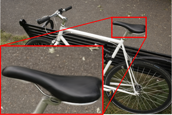
(a) w/o per-tile depth

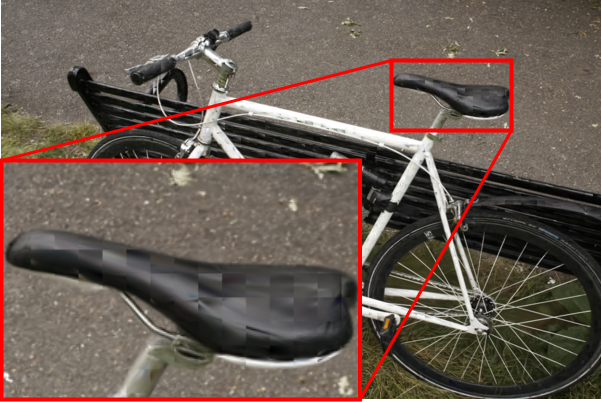
(b) w/ naïve per-tile depth

Figure 4. Comparison of 3DGS with and without per-tile depth calculation. Per-tile depth calculation lowers sorting errors ($\delta_{max}=4.01,\delta_{avg}=0.284$ compared to $\delta_{max}=5.43,\delta_{avg}=0.898$). However, doing this without additional per-pixel sorting leads to artifacts at the tile borders.

Although it is not possible to describe $t_{opt}$ with a simple primitive for rasterization, we may still rely on the fact that $t_{opt}$ is smooth across neighboring rays. As such, the sorting order of neighboring rays should also be similar. Because sorting in 3DGS already happens with a combined tile/depth key, we could replace the global depth with an accurate per-tile depth value for each Gaussian, e.g., using the tile center ray for Eqn. (4). As can be seen in Fig. 4, using per-tile depth clearly leads to artifacts along the tile borders.

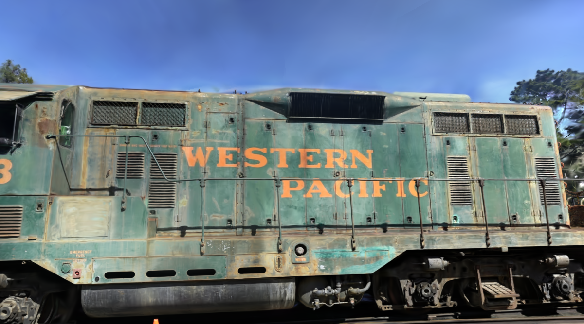
[C].02 full sorted [C].24 [C].24 [C].24 [C].24

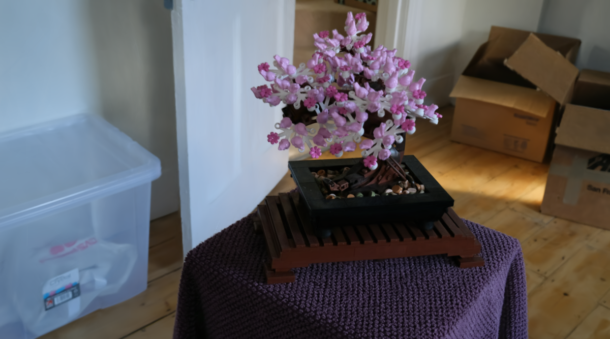
3DGS trained

Ours trained

3DGS trained

Ours trained

[C].02 3DGS rendered [C].19 [C].19 [C].19 [C].19 [C].19

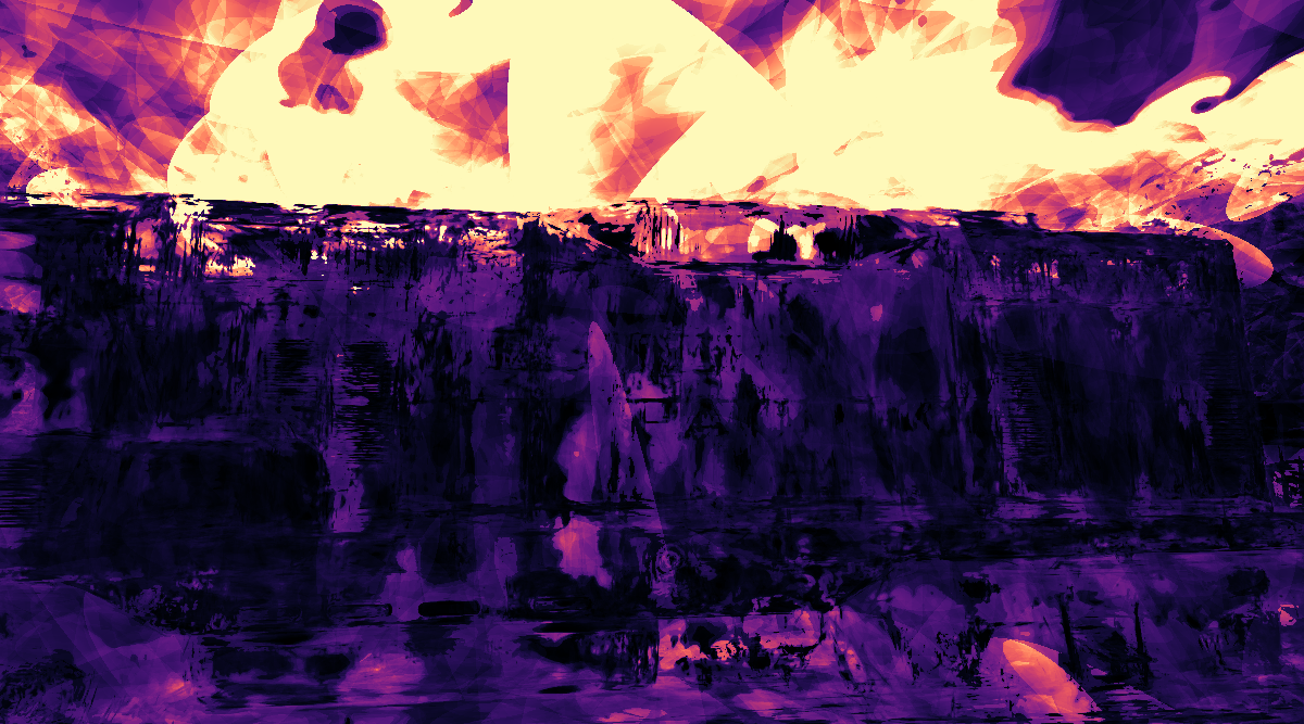
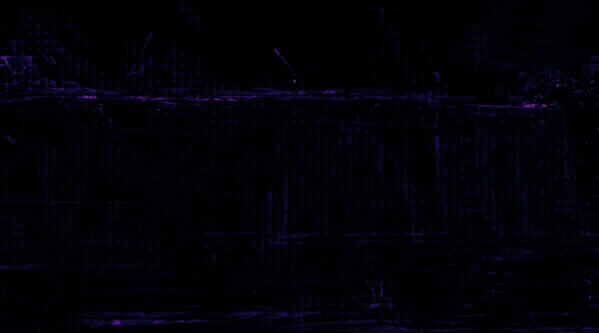
[C].02 Sort Error [C].19 [C].19 [C].19 [C].19 [C].19

[C].02 3DGS rendered [C].19 [C].19 [C].19 [C].19 [C].19

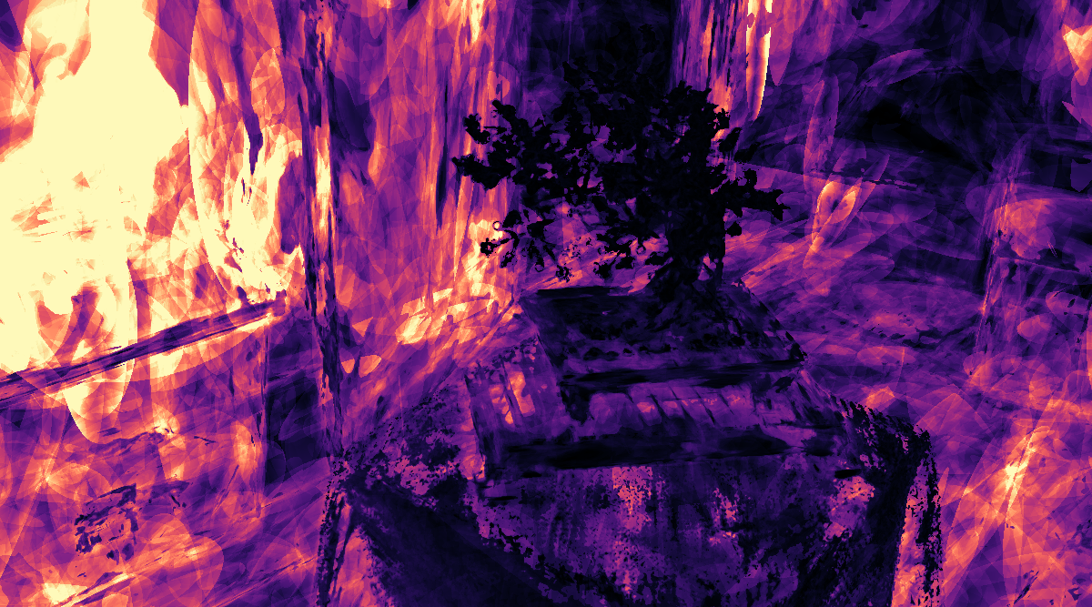
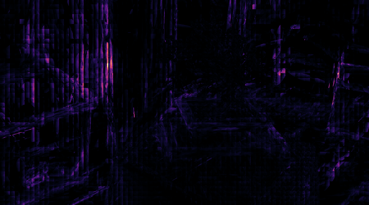
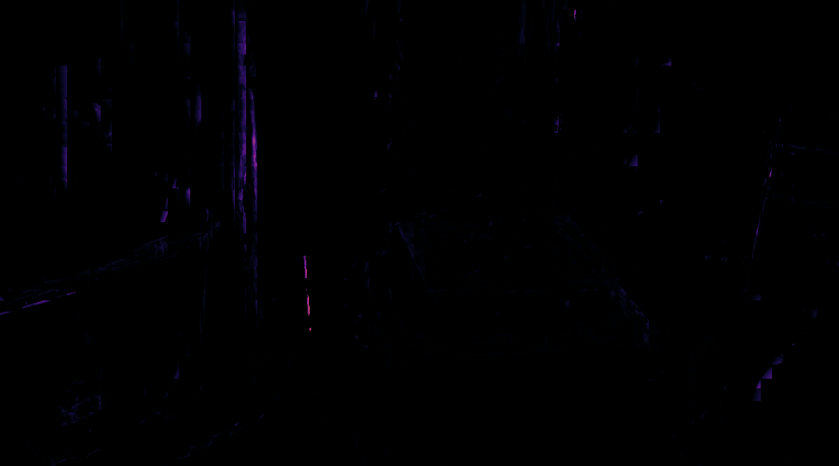
[C].02 Sort Error [C].19 [C].19 [C].19 [C].19 [C].19

full sort

3DGS

resort 4

resort 24

Ours

[b] 0 10.0

Figure 7. Correct rendering of a trained 3DGS scene with per-pixel sorting reveals how 3DGS cheats with the location of Gaussians. Our approach, on the other hand, considers correct sorting during training and rendering. Below, we show the sort error of different resorting windows and our full approach cf. Tab. 1. We intentionally use the trained 3DGS model here, as our trained version does not show these kinds of artifacts for visualization. The error visualization captures the sum over the depth difference of all wrongly sorted neighbors. For resorting with a window size of 4, tile artifacts are still visible. Our approach hardly diverges from fully sorted rendering, while running $100\times$ faster; it is also about $5\times$ faster than resort 24 and on average only 4% slower than 3DGS.

With that in mind, we propose a simple per-ray resorting extension. Instead of immediately blending the next Gaussian when walking through the tile list, we keep a small resorting window in registers. When loading a Gaussian, we evaluate its $t_{opt}$ and use insertion sort to place it in the resorting window. If the window overflows, we blend the sample with the smallest depth. Although this sorting strategy is easy to implement, it already achieves good results for a resorting window of about $16$ to $24$, removing the majority of visible popping artifacts in our tested scenes. To confirm the improvement in blending order, we compute a per-ray sort error $\delta$: If two consecutive Gaussians are out of order, we accumulate their difference in $t_{opt}$, detailed in Tab. 1 and Fig. 7. As can be seen, there is a non-negligible cost even for such a simple approach.

Table 1. Maximum sort error over all pixels and average sort error for two representative example views from Fig. 7. A full sort per ray increases rendering times (relative to 3DGS) by more than $100\times$. Local resorting with a sort window of $16$ to $24$ removes the majority of visible popping artifacts, yet increases rendering time $2$ to $6\times$. Our hierarchical approach improves sort quality further and keeps processing time low. Note that a larger sorting window may lead to more Gaussians being fetched and thus our measurement of $\delta_{\text{max}}$ may increase with larger sort windows.

		3DGS	Full	Resorting Window				Ours
				4	8	16	24
Train	$\delta_{\text{max}}$	28.445	0.000	5.867	3.882	3.544	4.580	0.575
	$\delta_{\text{avg}}$	3.688	0.000	0.124	0.045	0.014	0.007	0.003
	time[ms]	1.00	142.03	1.21	1.66	2.70	4.22	0.92
Bonsai	$\delta_{\text{max}}$	33.543	0.000	12.786	8.954	6.391	5.595	3.098
	$\delta_{\text{avg}}$	3.786	0.000	0.265	0.110	0.039	0.019	0.006
	time[ms]	1.00	179.70	1.76	2.58	4.33	6.88	1.47

3.4. Hierarchical Rendering

Local resorting is already able to significantly improve the per-pixel sort order, which greatly reduces popping artifacts. To tackle the imposed performance overhead, we insert additional resorting levels between tiles and individual threads, creating a sort hierarchy. In this way, we can share sorting efforts between neighboring rays, while incrementally refining the sort order as we move towards individual rays. By additionally culling non-contributing Gaussians at every level of the hierarchy, we can drastically reduce sorting costs. We propose a hierarchical rendering pipeline that relies on the innate memory and execution hierarchy of the GPU to minimize the number of memory access operations, as outlined in Fig. 6. For a fair comparison, we intentionally only alter the blend order of Gaussians and leave the other parts of 3DGS untouched, including the 2D splatting approximation from Zwicker et al. (2002).

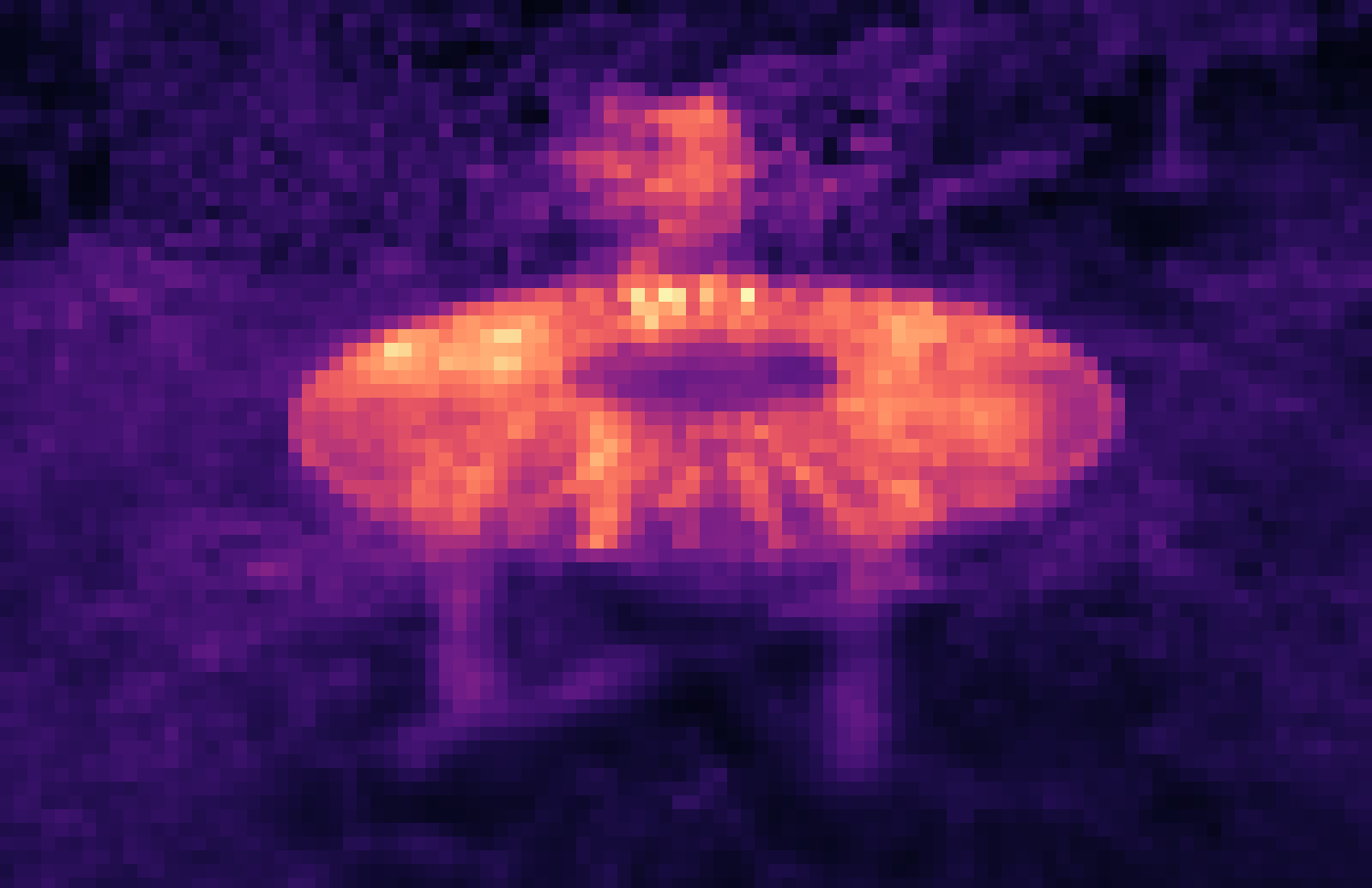
(a) w/o culling

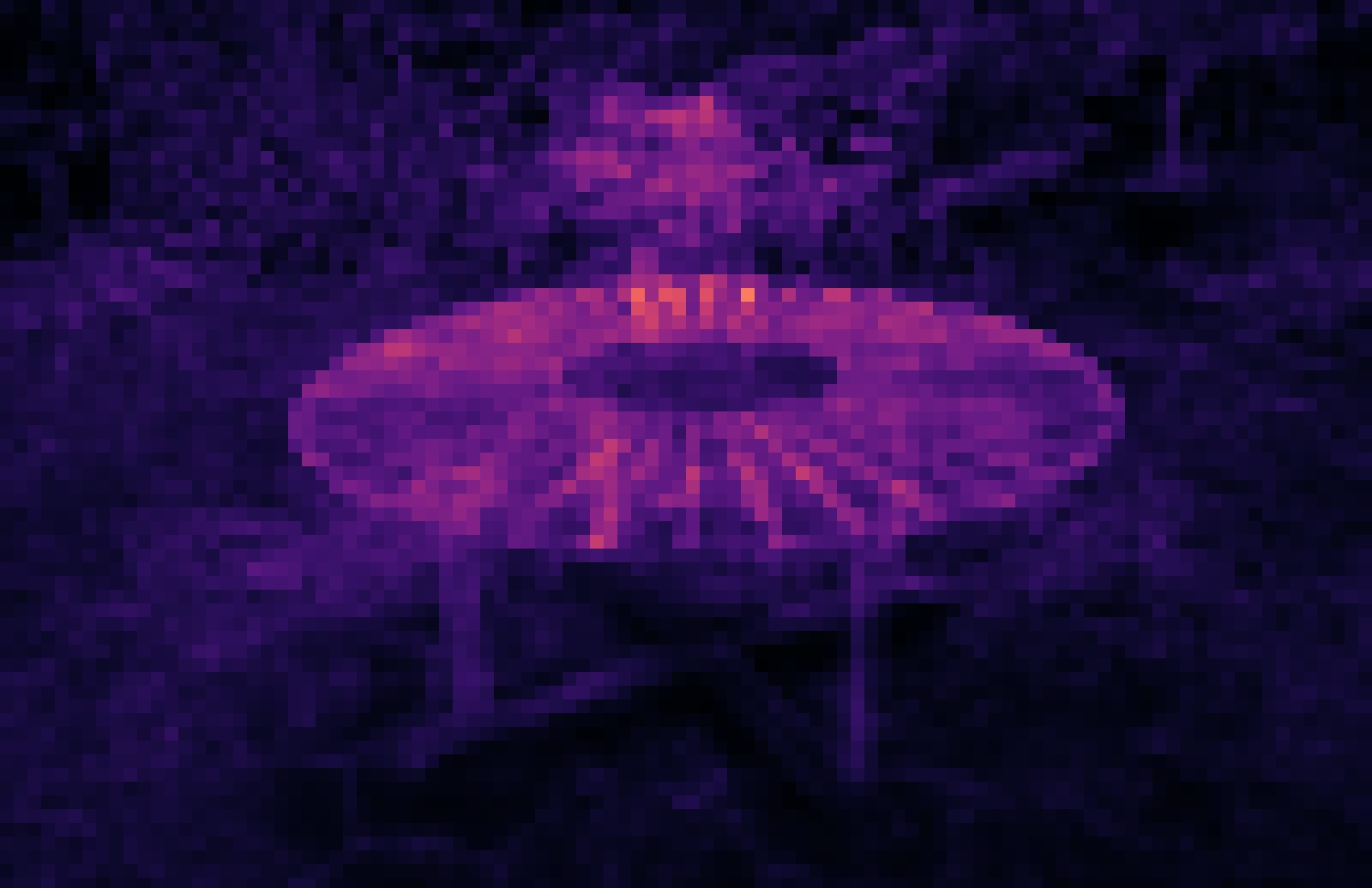
(b) w/ culling

0       5k

Figure 5. Number of Gaussians per tile with and without per-tile culling enabled for the Mip-NeRF 360 garden scene. The average number of Gaussians per tile is reduced by $\sim 44\%$.

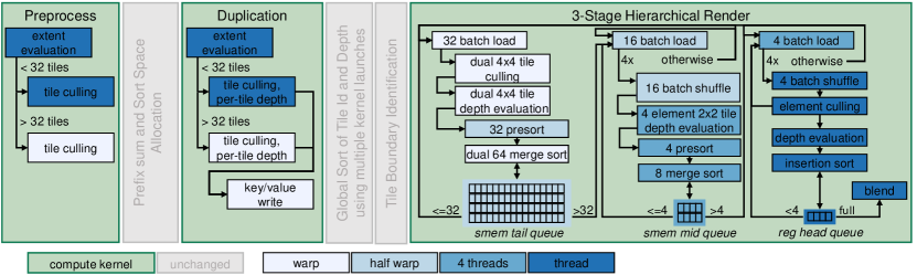
Figure 6. Overview of the detailed steps in our pipeline. We add load balancing, tile culling and per-tile depth evaluation to the first two stages of 3DGS. Our hierarchical rasterizer utilizes three sorted queues, going from $4\times 4$ tiles over $2\times 2$ tiles to individual rays. Depending on the queue fill levels, we switch between different cooperative group sizes while ensuring the queues remain filled for appropriate sorting. Our pipeline achieves an effective sorting window of 25-72 elements, depending on the current queue fill levels.

Tile-based culling

We propose a fast tile-based culling approach that bounds Gaussians to exactly those tiles they contribute to. For each ray, Kerbl et al. (2023) disregard Gaussians with a contribution below $\epsilon_{O}=1/255$, which forms an exact culling condition. Like 3DGS, we start with an axis-aligned bounding rectangle using the largest eigenvalue of the 2D covariance matrix to determine which tiles may potentially be touched during both Preprocess and Duplication. This conservative estimate gives very large bounds for highly anisotropic Gaussians.

For exact culling, we then calculate the point $\mathbf{\hat{\mathbf{x}}}$ inside each tile $X$ that maximizes the 2D Gaussian’s contribution $G_{2}(\mathbf{x})$:

(5) $$\mathbf{\hat{\mathbf{x}}}=\operatorname*{arg\,max}_{\mathbf{x}\in X}G_{2}(\mathbf{x})=\operatorname*{arg\,min}_{\mathbf{x}\in X}(\mathbf{x}-\mathbf{\mu_{2}})^{T}\Sigma_{2}^{-1}(\mathbf{x}-\mathbf{\mu_{2}}).$$

If $\mu_{2}\in X\Rightarrow\mathbf{\hat{\mathbf{x}}}=\mathbf{\mu_{2}}$. If $\mu_{2}\notin X$, then $\mathbf{\hat{\mathbf{x}}}$ must lie on one of the two tile edges closest to $\mu_{2}$, due to Gaussians being monotonic along rays pointing away from $\mathbf{\mu_{2}}$. We can then perform line search along those edges and clamp the resulting values to obtain ${\hat{\mathbf{x}}}$ (see the supplementary material for the full algorithm). Finally, we evaluate $G_{2}(\mathbf{\hat{\mathbf{x}}})$ to perform the comparison with $\epsilon_{O}$, which significantly reduces the number of Gaussians per tile (cf. Fig. 5).

Tile-depth Adjustment

For pre-sorting we require a representative $t_{opt}$ per tile. Intuitively, the center ray of the tile should be a valid compromise for all rays in the tile. However, this completely ignores the fact that a Gaussian in general does not uniformly contribute to all rays in a tile. Especially for small Gaussians whose main extent is approximately parallel to the view rays, the center ray may result in depth estimates far away from any contribution made by the Gaussian.

Arguably, the weighted integral $\int_{X}G_{2}(\mathbf{x})t_{opt}(\mathbf{x})d\mathbf{x}$ is a better estimate. Yet, even a numerical approximation considering all rays in the tile $X$ is too compute-intensive. Thus, we approximate it with a single sample: the one with the highest weight within a tile, i.e., $\mathbf{\hat{\mathbf{x}}}$. Since $\mathbf{\hat{\mathbf{x}}}$ was already calculated during culling, we only need to construct the corresponding ray to evaluate $t_{opt}$. The optimized depth location reduces $(\delta_{\text{max}},\delta_{\text{avg}})$ from $(1.553$, $0.006)$ to $(0.575$, $0.003)$ and $(3.917$, $0.014)$ to $(3.098$, $0.006)$ for the views in Tab. 1.

Load Balancing

Similar to other compute-mode rasterization methods, primitives that cover a large portion of the screen may become an issue if a single thread evaluates their coverage. For 3DGS, this is the case in the first two stages of the rendering pipeline, which operate on a per-Gaussian basis. For our method, tile-culling and per-tile depth calculations increase the workload of these stages, which further amplifies this problem.

To remedy this issue, we propose a two-stage load balancing scheme: In the first phase, each thread responsible for a Gaussian which covers fewer than a predetermined maximum number of tiles, performs its own processing. We empirically determined that a maximum of $32$ results in good performance. Most threads are typically idle after this initial phase. In the second phase, we distribute the remaining workload within each warp using warp voting and shuffle instructions. Especially for close-ups, our approach can speed up Preprocess and Duplication by up to $10\times$.

Hierarchically Sorted Rendering

With the goal of establishing a hierarchical rendering approach, relying on one kernel per hierarchy level may seem attractive. However, such an approach would require communication via slow global memory between the levels and would prohibit early ray termination after reaching the opacity threshold. Thus, we opt for combining the final three levels of our rendering hierarchy in a single kernel, where multiple threads cooperatively sort and manage shared queues, as detailed in Fig. 6. We use a large tail-queue of 64 elements for $4\times 4$ tiles (managed by 16 threads), feeding into four eight-element mid-queues, each representing a $2\times 2$ tile. Finally, each $2\times 2$ tile feeds into four head-queues with four elements, each being kept for a single ray and managed by one thread. For one $16\times 16$ tile, we thus start 256 threads, allocate 16 tail-queues and 64 mid-queues in shared memory as well as one head-queue per thread in registers.

The queues follow a push methodology to keep queue fill rates as high as possible, to ensure that resorting remains effective. While 16 threads (a halfwarp) are assigned to each tail-queue, we load and feed batches of 32 into tail-queues at once, allowing all threads within a warp to load data together. Thus, each thread is responsible for inserting Gaussians into two tail-queues. At first, each thread performs tile culling (as described before, just for a $4\times 4$ tile), followed by computing $t_{opt}$. For culled Gaussians, we set $t_{opt}=\infty$. Then, each halfwarp sorts the 32 newly loaded elements using Batcher Merge Sort (Batcher, 1968) before writing them to the back of the tail-queue. Typically, there are now two individually sorted parts in the tail-queue: the already present elements (up to 32) and the newly added (up to 32). As both are sorted, we use efficient merge sort to combine them. Culled Gaussians are now at the back of the queue and we can discard them.

While there are more than 32 elements in the tail-queue, we push batches of size 16 into the mid-queues. Each thread in the halfwarp re-fetches the data needed for computing $t_{opt}$ for a single Gaussian. Each group of four threads then pushes sub-batches of size four into their mid-queue, relying on shuffle instructions to update $t_{opt}$ for the $4\times 4$ tile. We follow the same approach as before: first we sort the four new entries according to depth, for which we use a simple coordination using shuffle instructions. We then use merge sort to combine the new elements with the existing ones.

After the mid-queue is filled, we draw four elements from it and insert them into the head-queue. Again, we batch-load the needed data using the four threads assigned to the respective mid-queue, and again use shuffle instructions to communicate all relevant information for each Gaussian to all other threads in the $2\times 2$ tile. We evaluate $t_{opt}$ and $\alpha$ for the respective rays and insert the newly computed data into the head-queue. If the Gaussian’s $\alpha$ is below $\epsilon_{O}$, we simply discard it. As we add elements one by one into the head-queue, we rely on simple insertion sort. Only if the head-queue is full, we take one element from it and perform blending, freeing up space for the next element from the mid-queue.

Due to the hierarchical structure, we effectively construct an overall sort window varying between $24$ and $72$, where the minimum is hit if the tail-queue is drained down to $17$ elements, $4$ elements each remain in mid and head. $72$ elements are sorted if we fill the tail-queue $64$ elements and then move $4$ elements through the half-filled mid-queue and the filled head-queue. While our sort setup typically achieves better sorting than a simple per-thread sort window of $24$, we may occasionally achieve worse sorting, as the lower queues are shared between threads.

3.5. Backward Pass

Contrary to 3DGS, we perform gradient computations in front-to-back blending order, avoiding the large memory overhead required for storing per-ray sorted Gaussians—which would be needed to restore the correct blending order (cf. supplemental for details). In our experiments, this did not impact the stability of the gradient computations.

Table 2. Image metrics for our method, 3DGS and related work. Results with dagger ($\dagger$) are reproduced from Kerbl et al. (2023) to facilitate cross-method comparisons. Our quality is comparable to 3DGS. With Opacity Decay, our approach loses slightly less quality than 3DGS.

Dataset	Deep Blending				Mip-NeRF 360 Indoor				Mip-NeRF 360 Outdoor				Tanks & Temples
Metric	PSNR$\uparrow$	SSIM$\uparrow$	LPIPS$\downarrow$	$\reflectbox{F}LIP$$\downarrow$	PSNR$\uparrow$	SSIM$\uparrow$	LPIPS$\downarrow$	$\reflectbox{F}LIP$$\downarrow$	PSNR$\uparrow$	SSIM$\uparrow$	LPIPS$\downarrow$	$\reflectbox{F}LIP$$\downarrow$	PSNR$\uparrow$	SSIM$\uparrow$	LPIPS$\downarrow$	$\reflectbox{F}LIP$$\downarrow$
(Barron et al., 2022) $\dagger$	29.40	0.900	0.245	0.138	31.57	0.914	0.182	0.088	24.42	0.691	0.286	0.170	22.22	0.758	0.256	0.232
(Müller et al., 2022)$\dagger$ (base)	23.62	0.797	0.423	0.258	28.65	0.840	0.281	0.120	22.63	0.536	0.444	0.203	21.72	0.723	0.330	0.245
(Müller et al., 2022)$\dagger$ (big)	24.96	0.817	0.390	0.222	29.14	0.863	0.241	0.114	22.75	0.567	0.403	0.200	21.92	0.745	0.304	0.241
(Fridovich-Keil et al., 2022)$\dagger$	23.09	0.794	0.425	0.244	24.84	0.765	0.366	0.182	21.69	0.513	0.467	0.229	21.09	0.719	0.344	0.262
3DGS	29.46	0.900	0.247	0.131	30.98	0.922	0.189	0.094	24.59	0.727	0.240	0.167	23.71	0.845	0.178	0.199
Ours	29.86	0.904	0.234	0.127	30.62	0.921	0.186	0.099	24.60	0.728	0.235	0.167	23.21	0.843	0.173	0.216
3DGS (Opacity Decay)	28.94	0.894	0.262	0.134	30.57	0.918	0.198	0.097	24.45	0.718	0.261	0.169	23.52	0.839	0.194	0.205
Ours (Opacity Decay)	29.84	0.905	0.241	0.126	30.03	0.917	0.194	0.103	24.46	0.722	0.254	0.169	23.18	0.839	0.184	0.214

Table 3. View-consistency metrics for videos. We measure $\text{\reflectbox{F}LIP}_{t}$ for timesteps $t=1,t=7$ (lower is better). Our method outperforms 3DGS with and without Opacity Decay.

Dataset	DB		M360 Indoor		M360 Outdoor		T&T
Metric	$\text{\reflectbox{F}LIP}_{1}$	$\text{\reflectbox{F}LIP}_{7}$	$\text{\reflectbox{F}LIP}_{1}$	$\text{\reflectbox{F}LIP}_{7}$	$\text{\reflectbox{F}LIP}_{1}$	$\text{\reflectbox{F}LIP}_{7}$	$\text{\reflectbox{F}LIP}_{1}$	$\text{\reflectbox{F}LIP}_{7}$
	Without Opacity Decay
3DGS	0.0061	0.0114	0.0069	0.0134	0.0083	0.0148	0.0102	0.0286
Ours	0.0053	0.0059	0.0060	0.0077	0.0085	0.0122	0.0076	0.0113
	With Opacity Decay
3DGS	0.0063	0.0122	0.0072	0.0149	0.0083	0.0154	0.0107	0.0315
Ours	0.0052	0.0055	0.0060	0.0073	0.0083	0.0115	0.0076	0.0114

4. Evaluation

For evaluation, we follow Kerbl et al. (2023) and use 13 real-world scenes from Mip-NeRF 360 (Barron et al., 2022), Deep Blending (Hedman et al., 2018) and Tanks & Temples (Knapitsch et al., 2017).

Opacity Decay

A viable approach to reduce the total number of Gaussians after optimization is replacing 3DGS’s opacity reset with a standard Opacity Decay during training. Every $50$ iterations, we multiply each Gaussian’s opacity with a constant $\epsilon_{\text{decay}}=0.9995$. We find that this modification results in significantly fewer, but larger Gaussians, potentially causing exacerbated popping.

4.1. Quantitative Evaluation

Image Metrics

For our quantitative evaluation, we report PSNR, SSIM, LPIPS (Zhang et al., 2018) and F LIP (Andersson et al., 2020) in Tab. 2. For Deep Blending and Mip-NeRF 360 Outdoor, we outperform 3DGS. For Tanks & Temples and Mip-NeRF 360 Indoor, our model performs slightly worse, which we attribute to 3DGS’s ability to fake view-dependent effects with popping. When enabling Opacity Decay, which results in 50% fewer Gaussians, our method retains more quality than 3DGS. In general, our approach performs comparably to 3DGS in terms of standard image quality metrics.

Popping

View inconsistencies between subsequent frames, such as popping, cannot be detected with standard image quality metrics. To detect such artifacts, we follow recent best practice in 3D style transfer (Nguyen-Phuoc et al., 2022) and measure consistency between novel views and warped novel views with optical flow (Lai et al., 2018). For our method and 3DGS, we capture videos from three separate camera paths per scene, exhibiting both rotation and translation. We then warp each frame $\mathbf{F}_{i}$ to a subsequent frame $\mathbf{F}_{i+t}$ using optical flow predictions from RAFT (Teed and Deng, 2020).

Measuring the error between warped frame $\hat{\mathbf{F}}_{i+t}$ and the actual frame $\mathbf{F}_{i+t}$ with MSE does not prove effective to detect popping artifacts. MSE tends to weigh small inaccuracies that originate from warping higher than popping artifacts. F LIP (Andersson et al., 2020) proves significantly more reliable in our experiments, as it approximates the difference perceived by humans when flipping between images. For each frame, we calculate a consistency error $E_{i+t}=\text{\reflectbox{F}LIP}(\hat{\mathbf{F}}_{i+t},\mathbf{F}_{i+t})$. For each video, consisting of $N$ frames, we then compute the mean F LIP error as

(6) $$\text{\reflectbox{F}LIP}_{t}=\frac{1}{N-t}\sum_{i=0}^{N-t}E_{i+t}.$$

Note that the error metric includes a base error floor due to dis-occlusions under translation and correct view-dependent shading. Thus, a zero score is not possible, and averages over all pixels and frames are considered. Therefore, low score differences may already point towards significant popping.

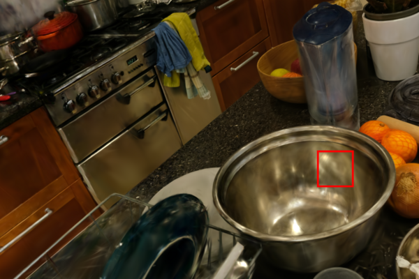
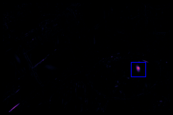
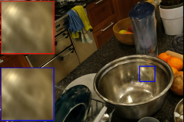
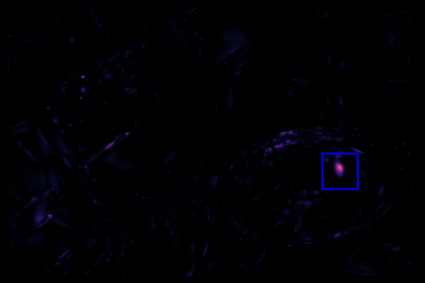
[C].02 3DGS [C].19 [C].19 [C].19 [C].19 [C].19

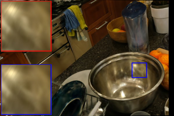
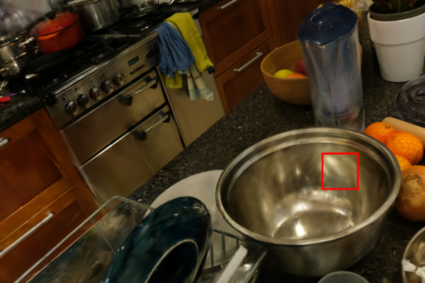
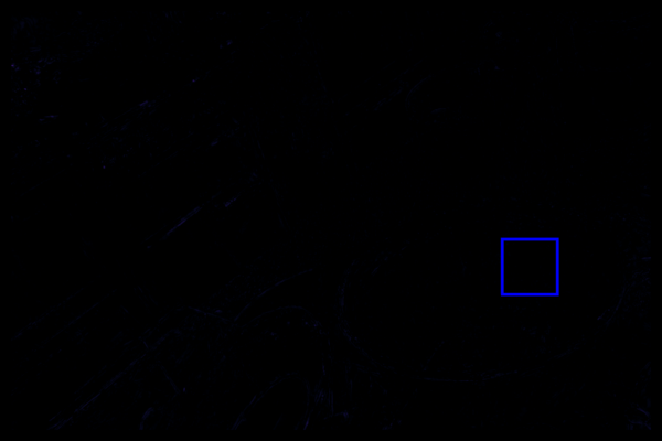
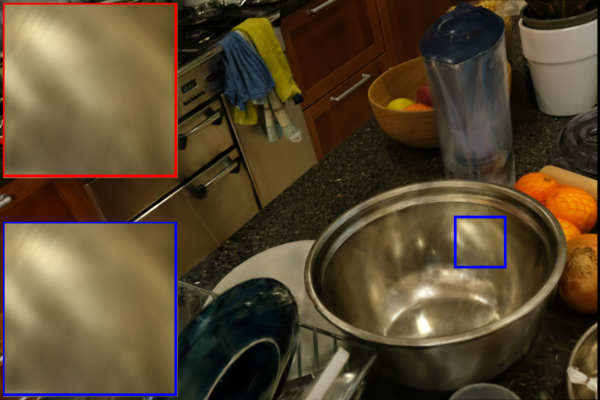
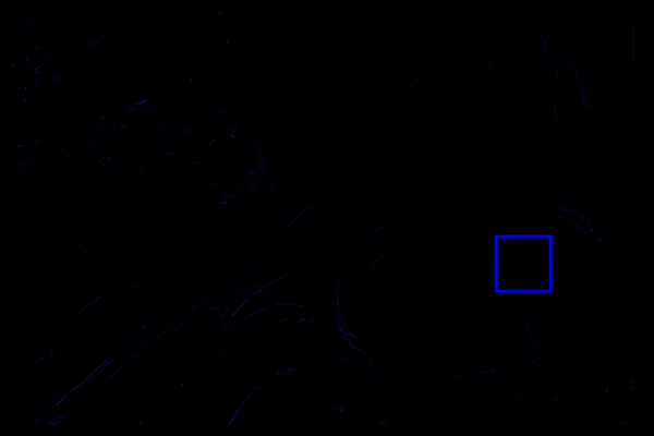
[C].02 Ours [C].19 [C].19 [C].19 [C].19 [C].19

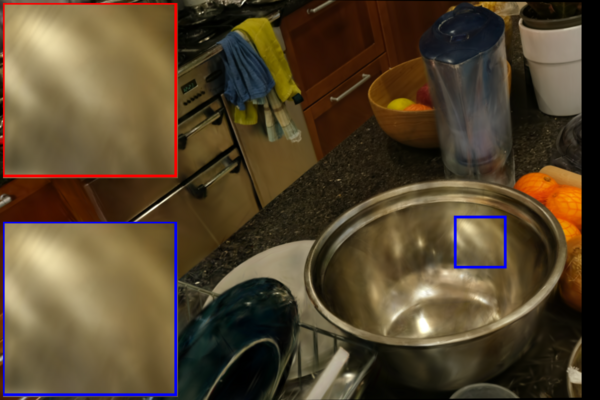
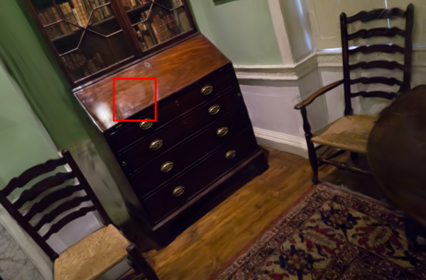
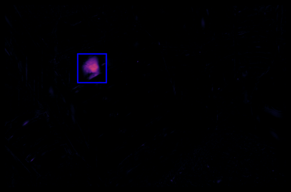
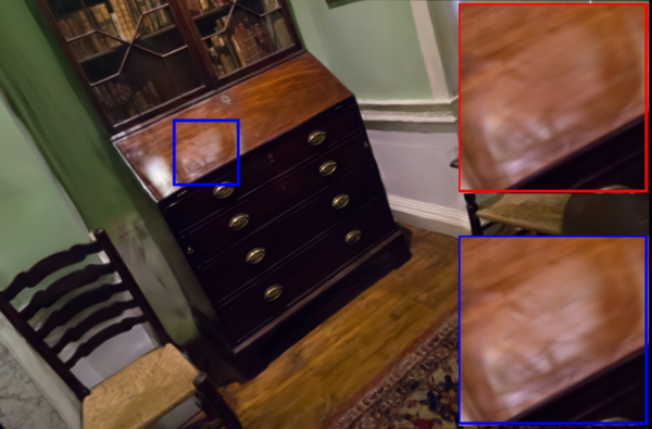
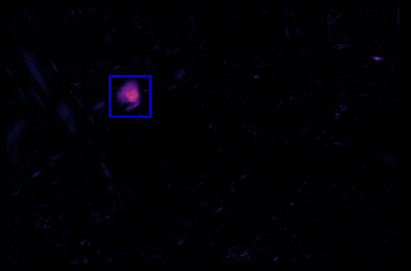
[C].02 3DGS [C].19 [C].19 [C].19 [C].19 [C].19

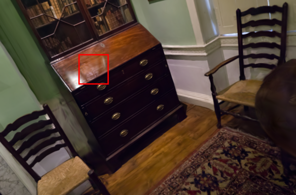
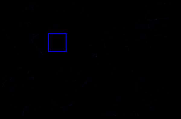
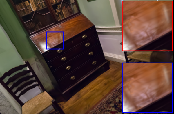
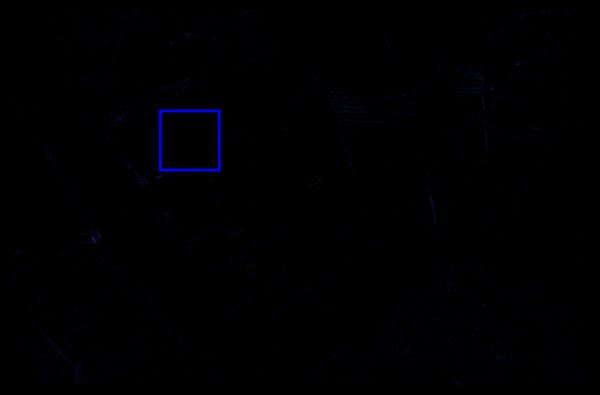
[C].02 Ours [C].19 [C].19 [C].19 [C].19 [C].19

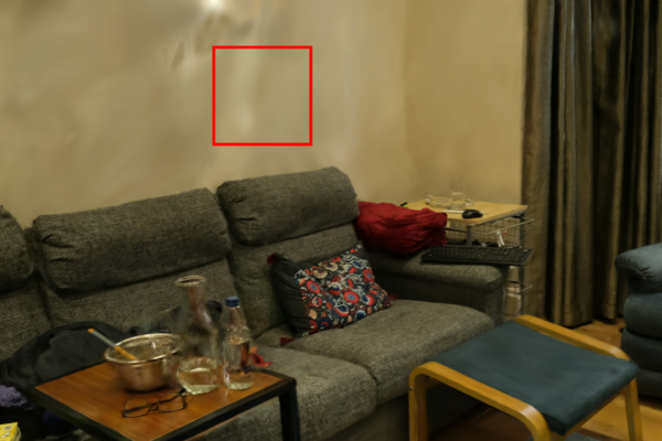
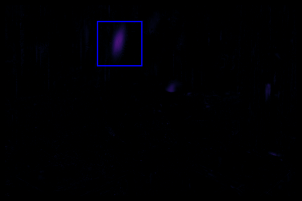
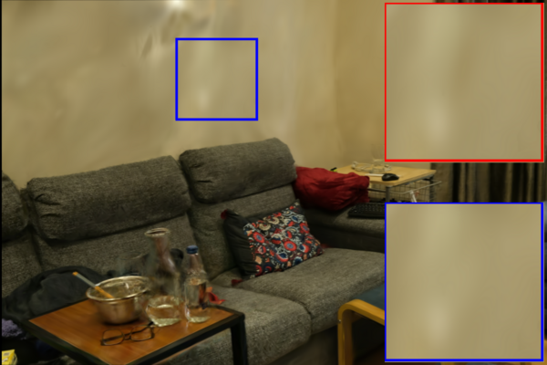
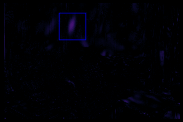
[C].02 3DGS [C].19 [C].19 [C].19 [C].19 [C].19

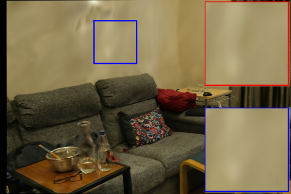
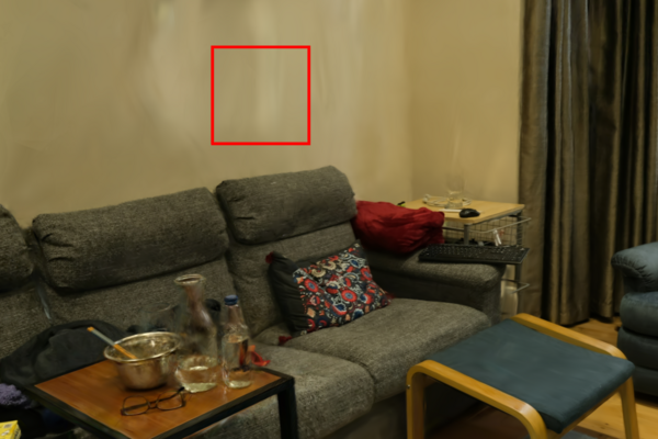
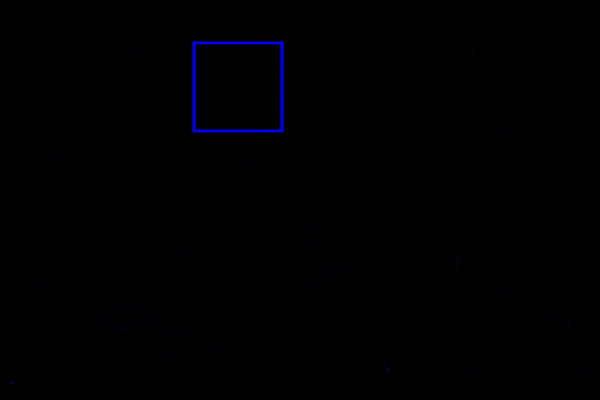
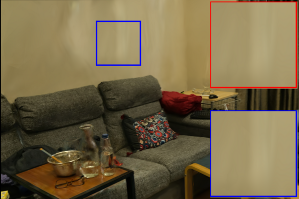
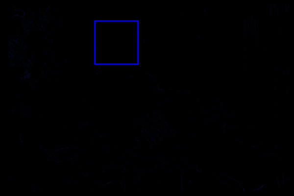
[C].02 Ours [C].19 [C].19 [C].19 [C].19 [C].19

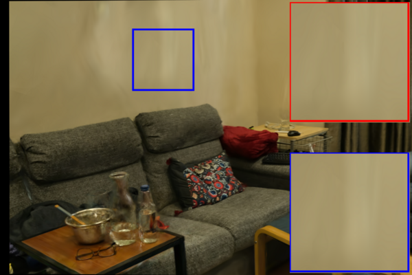
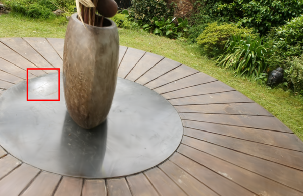
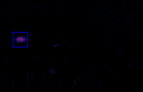
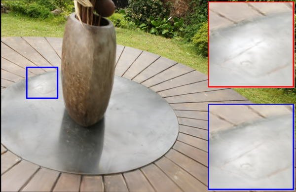
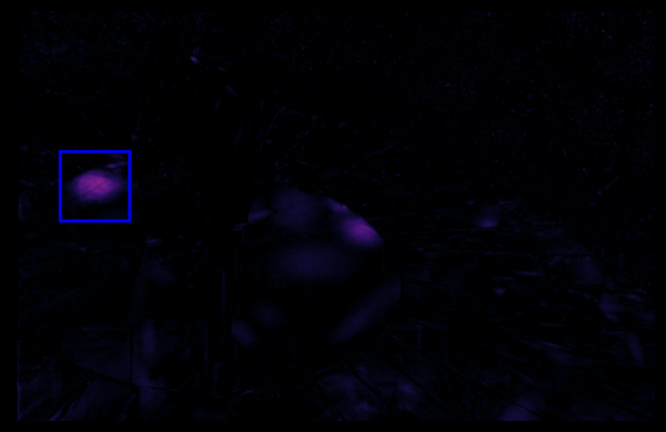
[C].02 3DGS [C].19 [C].19 [C].19 [C].19 [C].19

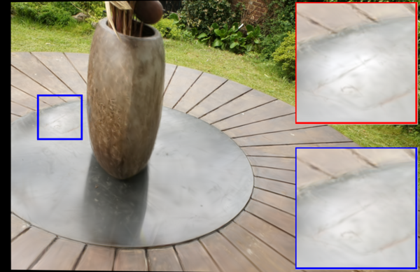
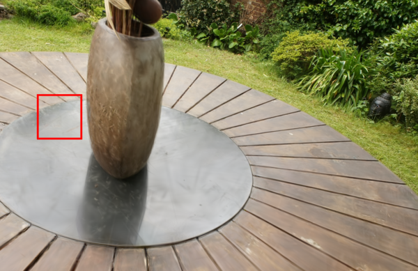
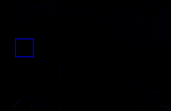
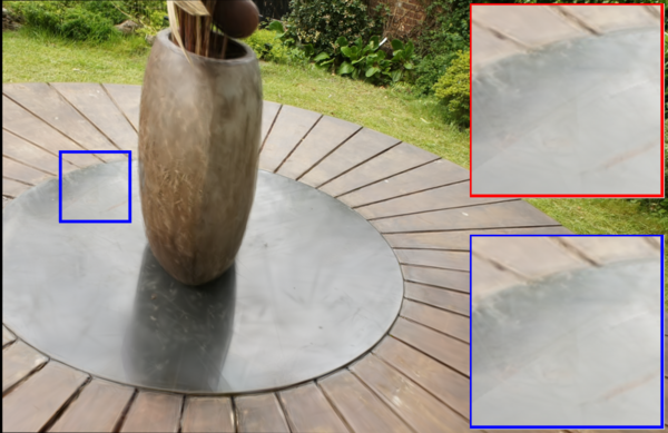
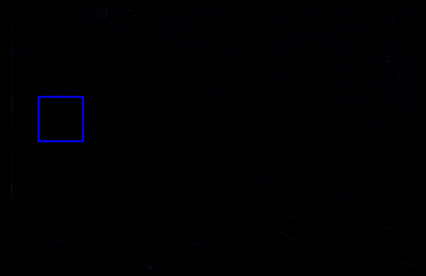
[C].02 Ours [C].19 [C].19 [C].19 [C].19 [C].19

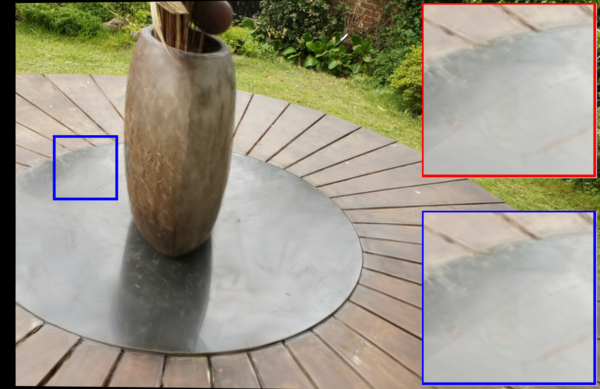
Figure 9. Visualization of our proposed popping detection method with detailed views inset. We warp view $\mathbf{F}_{i}$ to $\hat{\mathbf{F}}_{i+1},\hat{\mathbf{F}}_{i+7}$ using optical flow and use F LIP to measure errors between warped and non-warped views. While $\text{\reflectbox{F}LIP}_{1}$ is able to effectively detect popping artifacts, the obtained errors are only accumulated over a single frame. On the contrary, $\text{\reflectbox{F}LIP}_{7}$ is able to accumulate errors due to popping over multiple frames, making this metric more reliable.

We use $t=1$ and $t=7$ to measure short-range and long-range consistency, respectively. Tab. 3 shows our obtained results. Our method is more view-consistent than 3DGS, especially when looking at $\text{\reflectbox{F}LIP}_{7}$ results. We argue that $\text{\reflectbox{F}LIP}_{7}$ is a more reliable metric, allowing errors due to popping to accumulate over multiple frames, as can be seen in Fig. 9. Please see the supplementary video for further evidence. With Opacity Decay, our approach achieves virtually identical results, indicating that our method can handle large Gaussians. For 3DGS, popping is significantly increased, indicating that 3DGS may increase the number of Gaussians to hide imperfections in the renderer, while our approach achieves comparable view-consistency scores.

4.2. Qualitative Evaluation

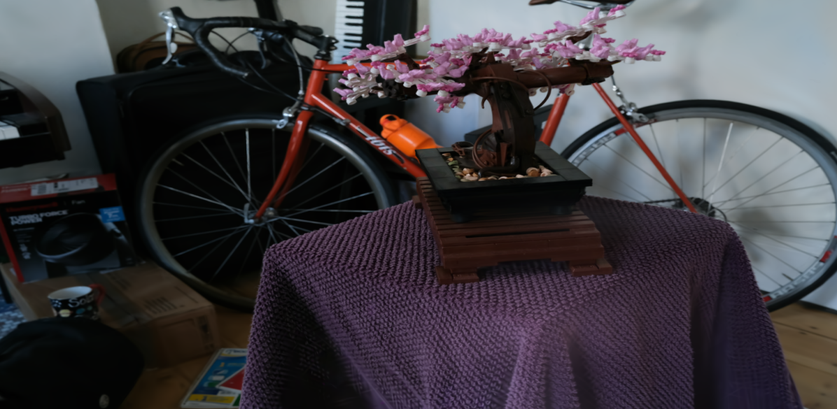
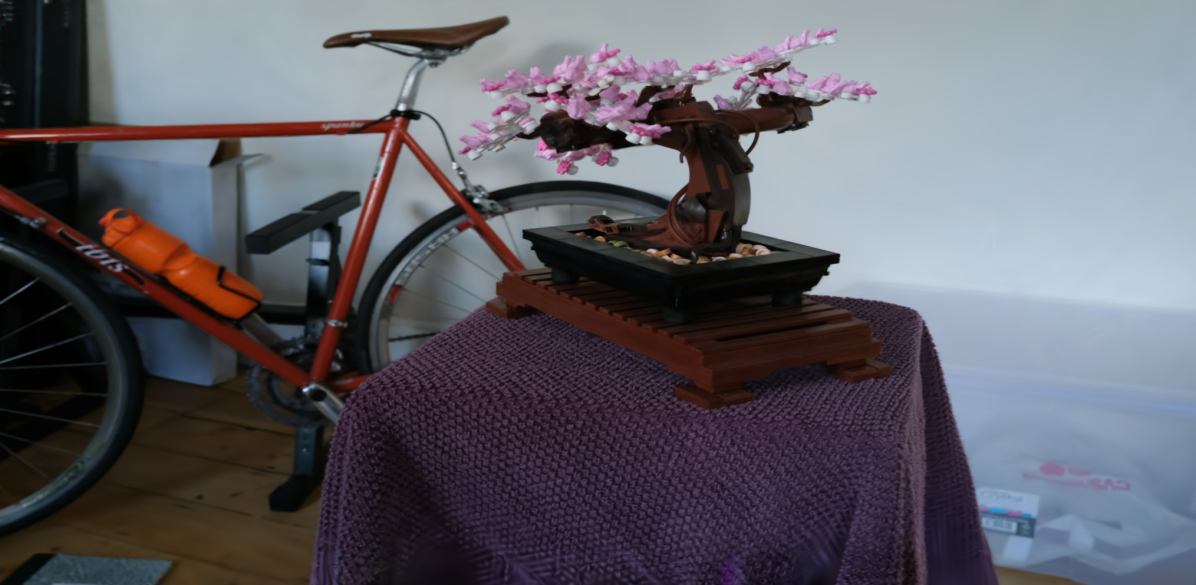
[C].02 3DGS [C].1575 [C].1575 [C].1575 [C].1575 [C].1575 [C].1575

[C].02 Ground Truth [C].1575 [C].1575 [C].1575 [C].1575 [C].1575 [C].1575

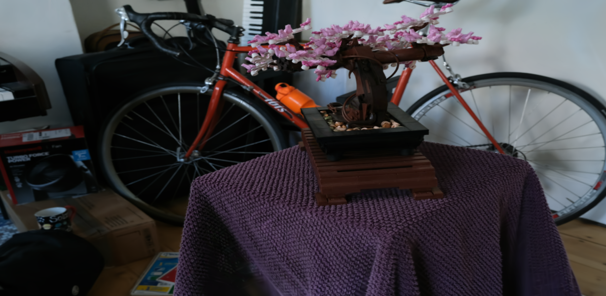
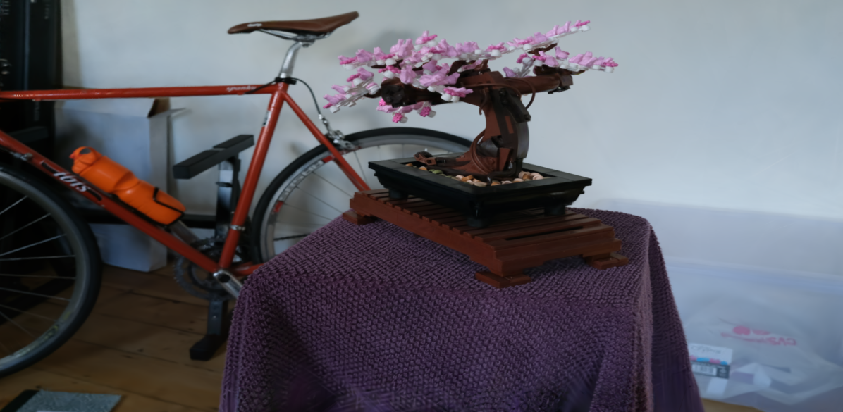
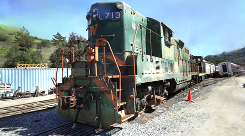
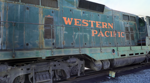
[C].02 Ours [C].1575 [C].1575 [C].1575 [C].1575 [C].1575 [C].1575

Ours PSNR^$\uparrow$

3DGS PSNR^$\uparrow$

Ours PSNR^$\uparrow$

3DGS PSNR^$\uparrow$

Ours PSNR^$\uparrow$

3DGS PSNR^$\uparrow$

Figure 8. Image comparisons of our method and 3DGS. In most configurations, our rendered images are virtually indistinguishable from 3DGS. For each scene, we show a result where our method performs better on the left, and a result where 3DGS performs better on the right.

To further complement our evaluation, we provide image comparisons in Fig. 8 and conduct a user study to verify the effectiveness of our approach and our proposed popping detection method.

4.2.1. User Study

18 participants were presented with pairs of videos from our approach and 3DGS, following the same camera path. The captured scenes exhibit rotation, translation, as well as a combination of the two. We instructed the participants to rate the videos concerning view-consistency and popping artifacts. The participants then indicated whether either of the techniques performed better or equal, which we translated into scores $s\in(-1,0,+1)$. On average, the results showed a clear preference for our approach ($s_{mean}=0.42$), which is statistically significant according to Wilcoxon Signed Rank tests ($Z=2276.5$, $p<.0001$). Details about the study can be found in the supplemental material.

4.3. Performance and Ablation

In Tab. 4 we show a performance comparison between 3DGS and our renderer with different configurations on an NVIDIA RTX 4090 with CUDA 11.8. The Render stage takes considerably longer for our hierarchical renderer (A-E) due to additional per-ray sorting. Not computing the per-tile depth (B) only marginally speeds up the Duplicate stage. Without our load balancing scheme (C), Duplicate takes 5$\times$ longer, as it is mostly dominated by very large Gaussians. Disabling tile-based culling (D) slightly accelerates Preprocess but leads to many more entries in the global sorting data structure, which increases Sort and Render times. Disabling hierarchical culling inside the render kernel (E) leads to a drastic increase in Render time as all Gaussians move through the entire pipeline. Our final approach (A) with all optimizations achieves competitive runtimes on all evaluated scenes. When training with Opacity Decay, both methods see a drastic performance increase, due to the significantly lower number of Gaussians—however while our approach stays view-consistent, 3DGS shows even more popping artifacts.

Table 4. Performance timings for different configurations of our method and 3DGS. Times in ms for Full HD resolution, averaged over 4 runs for all scenes with an interpolated camera path between all available COLMAP poses (30 frames per pose). The number of Gaussians is roughly the same for all methods (scene average $\sim 2.98\cdot 10^{6}$). Applying Opacity Decay during training leads to $\sim 50\%$ fewer Gaussians (scene average $\sim 1.54\cdot 10^{6}$).

Timings in ms	Preprocess	Duplicate	Sort	Render		Total
	Without Opacity Decay
3DGS	0.451	0.567	1.645	2.134		4.797
(A) Ours	0.649	0.437	0.301	3.599		4.986
(B) Ours w/o per-tile depth	0.658	0.283	0.301	3.599		4.841
(C) Ours w/o load balancing	0.847	2.059	0.415	3.505		6.827
(D) Ours w/o tile-based culling	0.610	0.479	1.180	5.346		7.614
(E) Ours w/o hier. culling	0.649	0.437	0.301	5.967		7.364
	With Opacity Decay
3DGS	0.215	0.378	0.626	1.059		2.276
Ours	0.366	0.223	0.161	2.227		2.976

The relative performance of our backward Render pass compared to 3DGS is only $1.1\times$ compared to the $1.5\times$ we see for the forward Render stage. This is mostly due to the backward Render executing a large number of atomics, which are equal between both approaches. Although the backward pass skips Duplicate and Sort—which are faster in our renderer—the final change in training time is only about 3%. The backward Render pass is only a single step in the entire training pipeline and thus, the overall time loss is close to negligible. Again, if we turn on Opacity Decay, training becomes proportionally faster.

5. Conclusion, Limitations, and Future Work

In this paper, we took a closer look at the way 3D Gaussian Splatting orders splats during blending. A detailed analysis of the splat’s depth computation revealed the reason for popping artifacts of 3DGS: the computed depth is highly inconsistent under rotation. A per-ray depth computation which considers the highest contribution along the ray as optimal blending depth, removes all popping artifacts but is $100\times$ more costly. With our hierarchical renderer, which includes multiple culling and resorting stages, we are only $1.03\times$ slower than 3DGS on average. While it is difficult to identify popping in standard quality metrics, we provided a view-consistency metric based on optical flow and F LIP, which shows that our approach significantly reduces popping. We could also confirm this fact in a user study. Furthermore, our approach remains view-consistent even when constructing the scene with half the Gaussians; for which 3DGS shows a significant increase in popping artifacts. As such, our approach can reduce memory by $2\times$ and render times by $1.6\times$ compared to 3DGS in this configuration, while reducing popping artifacts and achieving virtually indistinguishable quality.

While our approach typically removes all artifacts in our tests, resorting does not guarantee the right blend order, and thus could still lead to popping or flickering for very complex geometric relationships. Furthermore, our approach still ignores overlaps between Gaussians along the view ray. A fully correct volume rendering of Gaussians may not only remove artifacts completely but could lead to better scene reconstructions—a direction certainly worth exploring in the future.

[C].02 View $\mathbf{F}_{i}$ $\text{\reflectbox{F}LIP}_{1}$ Warped View $\hat{\mathbf{F}}_{i+1}$ $\text{\reflectbox{F}LIP}_{7}$ Warped View $\hat{\mathbf{F}}_{i+7}$

Appendix A Deriving Depth for 3D Gaussians along a Ray

In order to get an accurate depth estimate for our sort order of 3D Gaussians along a view ray $\mathbf{r}(t)=\mathbf{o}+t\mathbf{d}$, we perform a line search to find the $t_{opt}$ which maximizes the Gaussian’s contribution along the ray: $t_{opt}=\operatorname*{arg\,max}_{t}G(\mathbf{r}(t))$. This optimum can be found through the following derivation:

$$\frac{dG(\mathbf{r}(t))}{dt} =-\frac{1}{2}G(\mathbf{r}(t))\cdot\left((\mathbf{r}(t)-\mathbf{\mu})\Sigma^{-1}\mathbf{d}+\mathbf{d}^{T}\Sigma^{-1}(\mathbf{r}(t)-\mathbf{\mu})\right)$$

$$=-\frac{1}{2}G(\mathbf{r}(t))\cdot\left(2\cdot\mathbf{d}^{T}\Sigma^{-1}(\mathbf{r}(t)-\mathbf{\mu})\right)$$

$$=-G(\mathbf{o}+t\mathbf{d})\cdot\left(\mathbf{d}^{T}\Sigma^{-1}(\mathbf{o}+t\mathbf{d}-\mathbf{\mu})\right)=0$$

$$=\mathbf{d}^{T}\Sigma^{-1}(\mathbf{o}+t\mathbf{d}-\mathbf{\mu})=0$$

$$=\mathbf{d}^{T}\Sigma^{-1}\mathbf{d}\cdot t+\mathbf{d}^{T}\Sigma^{-1}(\mathbf{o}-\mathbf{\mu})=0$$

(7) $$t_{opt} =\frac{\mathbf{d}^{T}\Sigma^{-1}(\mathbf{\mu}-\mathbf{o})}{\mathbf{d}^{T}\Sigma^{-1}\mathbf{d}}.$$

The simplification from the first to the second line relies on the fact that $\Sigma^{-1}$ is symmetric and thus both expressions are identical. $\Sigma^{-1}$ can be efficiently computed:

$$\Sigma^{-1}=\left(RSSR^{T}\right)^{-1}=RS^{-1}S^{-1}R^{T}=R\begin{pmatrix}s_{x}^{-2}&0&0\\ 0&s_{y}^{-2}&0\\ 0&0&s_{z}^{-2}\end{pmatrix}R^{T}.$$

Appendix B Additional Implementation Details

This section contains a more thorough description of our implementation and various optimization strategies to make our hierarchical rasterizer viable for real-time rendering.

B.1. Tile-based Culling

In Algorithm 1, we describe how to find the maximum contributing point $\mathbf{\hat{\mathbf{x}}}$ of a 2D Gaussian $G_{2}$ parameterized by $\Sigma^{-1}_{2},\mathbf{\mu_{2}}$ inside an axis-aligned tile. If $\mathbf{\mu_{2}}$ lies inside the tile, then it is consequently also the maximum. Otherwise, the maximum has to lie on one of the two edges that are reachable from $\mathbf{\mu_{2}}$. Those are the two edges that originate from the tile corner point $\mathbf{\hat{\mathbf{p}}}$ closest to $\mathbf{\mu_{2}}$. We can then find the optimum by performing a line search along those two edges. By checking if $\mathbf{\mu_{2}}_{x},\mathbf{\mu_{2}}_{y}$ are in range of the tile in $x,y$ direction, as well as clamping the values of $t_{x},t_{y}$ to $[0,1]$, we ensure that the final point will lie on one of these two edges. The fact that the $y$ coordinate of $\mathbf{d_{x}}$ and the $x$ coordinate of $\mathbf{d_{y}}$ are zero, allows for further simplifications in the final implementation.

Data: $X=\{\forall\mathbf{x}\in\mathbb{R}^{2}|x_{\min}\leq\mathbf{x_{x}}\leq x_{\max}\land y_{\min}\leq\mathbf{x_{y}}\leq y_{\max}\}$

Result: $\mathbf{\hat{\mathbf{x}}}=\operatorname*{arg\,min}_{\mathbf{x}\in X}(\mathbf{x}-\mathbf{\mu_{2}})^{T}\Sigma_{2}^{-1}(\mathbf{x}-\mathbf{\mu_{2}})$

if $\mathbf{\mu_{2}}\in X$ then

       $\mathbf{\hat{\mathbf{x}}}\leftarrow\mathbf{\mu_{2}}$ ;

      

else

       $\mathbf{\hat{\mathbf{p}}}\leftarrow$ Corner closest to $\mathbf{\mu_{2}}$ ;

       $\mathbf{d_{x}},\mathbf{d_{y}}\leftarrow$ vectors to next AABB corners in $x,y$ direction ;

       $t_{x},t_{y}\leftarrow 0$ ;

       if $\mathbf{\mu_{2}}_{x}<x_{\min}\lor\mathbf{\mu_{2}}_{x}>x_{\max}$ then

             $t_{y}\leftarrow\min\left(1,\max\left(0,\frac{\mathbf{d_{y}^{T}}\Sigma^{-1}_{2}(\mathbf{\mu_{2}}-\mathbf{\hat{\mathbf{p}}})}{\mathbf{d_{y}^{T}}\Sigma^{-1}_{2}\mathbf{d_{y}}}\right)\right)$ ;

            

       end if

      

      if $\mathbf{\mu_{2}}_{y}<y_{\min}\lor\mathbf{\mu_{2}}_{y}>y_{\max}$ then

             $t_{x}\leftarrow\min\left(1,\max\left(0,\frac{\mathbf{d_{x}^{T}}\Sigma^{-1}_{2}(\mathbf{\mu_{2}}-\mathbf{\hat{\mathbf{p}}})}{\mathbf{d_{x}^{T}}\Sigma^{-1}_{2}\mathbf{d_{x}}}\right)\right)$ ;

            

       end if

      $\mathbf{\hat{\mathbf{x}}}\leftarrow\mathbf{\hat{\mathbf{p}}}+t_{x}\mathbf{d_{x}}+t_{y}\mathbf{d_{y}}$ ;

      

end if

$\Sigma^{-1}_{2},\mathbf{\mu_{2}}$: inverse covariance matrix and mean of 2D Gaussian $G_{2}$

$x_{\min},x_{\max},y_{\min},y_{\max}$: AABB dimensions

ALGORITHM 1 Finding maximum of 2D Gaussian inside AABB

$\Sigma^{-1}_{2},\mathbf{\mu_{2}}$: inverse covariance matrix and mean of 2D Gaussian $G_{2}$

$x_{\min},x_{\max},y_{\min},y_{\max}$: AABB dimensions

B.2. Tighter Bounding of 2D Gaussians

For computing the bounding rectangle of touched tiles on screen, Kerbl et al. (2023) first bound each 2D Gaussian with a circle of radius $r=3\cdot\lambda_{\max}$, where $\lambda_{\max}$ denotes the largest eigenvalue of the 2D inverse covariance matrix $\Sigma_{2}^{-1}$. They use a constant factor $t_{O}=3$ as a bound for a Gaussian, effectively clipping it at 1% of its peak value. We instead calculate an exact bound by considering the Gaussian’s actual opacity value $\alpha$ and compute $t_{O}=\sqrt{2\log(\frac{\alpha}{\epsilon_{O}})}$, which is itself upper bounded by ${t_{O}}_{\max}\approx 3.3209$ (since $\alpha\in[0,1]$). Therefore, we conclude that the bound of $t_{O}=3$ by Kerbl et al. (2023) was actually chosen too small for the opacity threshold $\epsilon_{O}=\frac{1}{255}$ used in the renderer. Additionally, our calculated bound allows us to fit a tighter circular bound around Gaussians with $\alpha<1$.

B.3. Global Sort

Using a giant global sort for all combined (tile/depth) keys seems wasteful. Sorting would be more efficient if the entries of each tile would be sorted individually, using a global partitioned sort. However, this requires all the entries of a tile to be continuous in memory, with each tile knowing the range of its respective entries. We can create such a setup by counting the number of entries per tile during the Preprocess stage with an atomic counter per tile and computing tile ranges with a prefix sum. In the Duplication stage, another atomic counter per tile can be used to retrieve offsets for each entry inside this range. While this reduces sorting costs to less than half in our experiments, the allocation using atomic operations adds an overhead that is about equal to the time saved in sorting. Thus, we opted to keep the original sorting approach.

Non-warped view $\mathbf{F}_{i+1}$

Warped $\hat{\mathbf{F}}_{i+1}$

$\text{\reflectbox{F}LIP}_{1}$

$\text{MSE}(\mathbf{F}_{i+1},\hat{\mathbf{F}}_{i+1})$

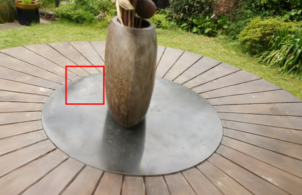
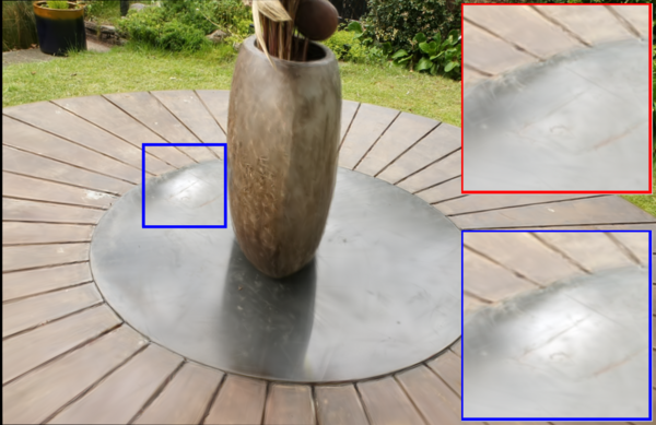
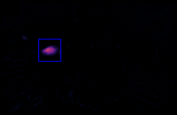
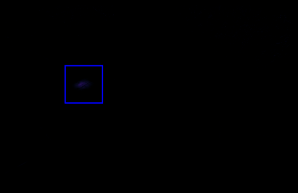
Figure 10. Comparison between F LIP and MSE to measure differences between non-warped frames $\mathbf{F}_{i+1}$ and warped frames $\hat{\mathbf{F}}_{i+1}$ for 3DGS. Notable, even egregious popping artefacts do not result in a large MSE for this specific frame. On the other hand, F LIP yields a large error.

B.4. Backward Pass

As mentioned before, our approach does not alter the actual blend routine employed by 3DGS, we only change the blend order. 3DGS performs blending and gradient computations back-to-front, which would require per-ray sort orders, resulting in an overly large memory overhead.

For gradient computation, it is not strictly necessary to iterate through the Gaussians in reverse blend order. We only require the Gaussian’s contribution to each ray $C(\mathbf{r})$ and the final accumulated transmittance $T_{N_{\mathbf{r}}}$, as well as the contributions of all other Gaussians blended before and after along the ray. Given that $C(\mathbf{r})$ is a sum and $T_{N_{\mathbf{r}}}$ is a product, we can store the final $C(\mathbf{r})$ and $T_{N_{\mathbf{r}}}$ from the forward pass and perform the same rendering routine during the backward pass, resulting in the same exact sort order. However, we now compute the gradients in the blend function: $C(\mathbf{r})$ up to the currently blended Gaussian is computed just like in the forward pass; the contribution of all Gaussians behind the currently blended is then computed via subtraction and division of $C(\mathbf{r})$ and $T_{N_{\mathbf{r}}}$ respectively. Note that this does not change the stability of the gradient computations in our experiments; 3DGS also relies on a division. One could argue that our approach may even lead to more accurate gradients as the Gaussians blended first along a ray have a higher contribution to the final color and computing those first, will accumulate less floating point errors compared to reversing the computation.

Also note that it is imperative that the same exact sort order is used between forward and backward pass to ensure correct gradients. Like 3DGS, we keep the global sort order in memory, which ensures that potentially equal depth values do not lead to different sorting results and thus the global sort does not need to be stable. In the hierarchical rasterizer implementation, we use stable sorting routines throughout: Batcher Merge Sort (Batcher, 1968) is stable by design, our merge sort routines rely on each thread’s rank to establish sort orders among equal depths, and our insertion sort is trivially stable.

B.5. Per-stage details

Preprocess and Duplication

Similarly to 3DGS, we also prepare common values for each Gaussian during Preprocess: We compute and store $G_{2}$ for every Gaussian, evaluate Spherical Harmonics relying on the direction from the camera to the Gaussians center as view direction, establish $\Sigma^{-1}$ relying on the specifics of $R$ and $S$, and precompute $\Sigma^{-1}(\mathbf{\mu}-\mathbf{o})$ for the current camera position $\mathbf{o}$, packing the 6 unique coefficients of $\Sigma^{-1}$ with the precomputed vector for efficient loading.

We found that activating “fast math” in combination with re-scheduling in Preprocess and Duplication may lead to slightly different ordering of floating point instructions. Thus, there may be slight differences in the number of tiles contributed by each Gaussian. As we already store the number of tiles contributed by every Gaussian for memory allocation, we rely on the following simple solution: during Preprocess we use a slightly lower threshold for culling, providing a slightly more conservative bound. During Duplication we recheck whether the right number of tile contributions have been written. If this is not the case, we simply add a dummy entry that sets a higher tile id and depth to $\infty$. For training, we suggest to disable “fast math”, ensuring that gradient computations are as stable as possible. However, for rendering using “fast math” may be beneficial to squeeze even more performance.

For load balancing in both Preprocess and Duplication, we rely on the ballot instruction to determine which threads still require computations. We use shuffle operations to broadcast already loaded register values, so each thread can perform culling and depth evaluation without additional memory loads. We assign successive potential tiles to each thread according to their thread rank in the warp. For every iteration of the inner loop we again ballot to determine which threads in the warp still want to write to a tile, i.e. did not cull away their tile. We can then mask all ballot bits of lower ranked threads, compute their sum via popc and determine the write location for each thread.

Render

Our hierarchical rasterizer is constructed from many steps, which are interleaved in their operation. Due to the setup, there are special optimizations we can perform based on the current state of the pipeline: The pipeline starts out with an initialize phase for each level, establishing a minimal fill level for each where no merge sort is performed. In this phase, blending is not taking place either. During the main operation, we ensure that we maintain a minimal fill level for each queue. Finally, the pipeline is drained where the number of elements in each queue will eventually drop to zero. Furthermore, we know that certain parts of the pipeline will always be executed a specific number of times. The combination of these facts allows for a significant amount of specialization and loop unrolling. However, we found that excessive code specialization and unrolling leads to a significant amount of stalls due to instruction fetches. Thus, relying on less specialized code is overall beneficial although up to 15% more instructions are required for the increased control logics.

For Batcher Merge Sort, we use a trival implementation adapted from the NVIDIA CUDA examples. For Merge Sort, we use a custom implementation that is adapted for our use case: each thread holds the to-be-inserted elements in registers and runs a binary search through the existing array to find where the new element should be placed with respect to the existing data. In combination with the thread’s rank, this yields the position in the final sorted array. Still, we need to update the position of the existing data. To this end, we switch the roles and memory locations of both data arrays and perform the exact same binary search, only switching strict comparison to non-strict comparison. Also note that we are operating on a small fixed size array, enabling loop unrolling and leading to very few memory accesses. For local presorting of four elements, we simply run three circular shuffles, revealing all elements among all threads to directly yield the right order via simple counting of smaller elements. In our tests this was faster than any other method.

As we reevaluate $t_{opt}$ many times for many different ray directions, constructing and normalizing view rays can become a bottleneck. Precomputing all view directions a single thread will need throughout the hierarchy (two for the tail queues, one for the mid queue and one for the head queue) would result in significant register pressure. Fortunately, the same directions are needed by different threads and we can store the directions in shared memory and fetch them on demand, leading to significant performance improvements.

Obviously, we need to take some care to ensure that threads do not diverge, especially, we can only retire queues if all threads in the associated tile are done. Also note that the loaded batches remain in registers for a potentially long time: a 16 batch loaded by a half warp remain in registers while four 4-thread batches are loaded and potentially up to 16 elements are blended. However, when the 32-wide batch is loaded, no smaller batches are kept alive, somewhat reducing register pressure.

Appendix C Popping Detection Metric

To mitigate errors due to occlusions, we use the occlusion detection method from Ruder et al. (2016). As we compute the optical flow for each model separately, we combine the derived occlusion masks for a fair comparison. In addition, we do not consider the outermost $20$ pixels for more stable predictions. To further enhance our metric, we subtract the per-pixel minimum $\reflectbox{F}LIP_{t}$ contribution before computing the mean over all pixels. It is easy to see that this does not change the inter-method difference. Finally, we use the RAFT (Teed and Deng, 2020) model pre-trained on SINTEL (Butler et al., 2012), which is publicly available.

In addition to the discussion presented in the main material, we provide a comparison between our proposed $\text{\reflectbox{F}LIP}_{1}$ and using MSE to measure errors between non-warped and warped views in Fig. 10. Evidently, F LIP is a much more reliable metric, considering the fact that a base error is unavoidable when using optical flow.

Appendix D User Study

For our user study we recruited 18 participants from a local university, age 26 to 34, all normal or corrected vision, no color blindness. All participants indicated that they are familiar with computer graphics (3-5 on a 5-point Likert scale).

We pre-recorded camera paths for all 13 scenes, looking at the main object present in the scene. For 3DGS and ours, we used the version specifically trained for these approaches without Opacity Decay. The paths all exhibit translation and rotation. The recorded video clips were between $8$ and $19$ seconds long.

After a pre-questionnaire, we instructed the participants that they will be presented with video pairs and they should specifically look for consistency in the rendering and then rate whether either of the video clips was more consistent than the other. If they did not consider any clip more consistent, they were allowed to rate them equal. We mapped those answers onto three values: ($-1$) 3DGS is more consistent, ($0$) they are equal, ($+1$) ours is more consistent. We presented both videos side-by-side and played them in a loop. We did not restrict the answer times, allowing participants to watch the clips multiple times. We randomized the order of videos (left, right) as well as the order of scenes.

Overall, participants considered our method more consistent in $54.3\%$ of the cases, voted for equal in $33.3\%$ and preferred 3DGS in $12.4\%$, leading to an average preference score of $s_{mean}=0.42$. The result is statistically significant according to Wilcoxon Signed Rank tests ($Z=2276.5$, $p<.0001$) (Woolson, 2008). As can be seen in Fig. 11, we observe inter-scene differences. For scenes with mostly small Gaussians, like in Bonsai or Kitchen, we expected less difference in the voted scores, as there is also less popping. In contrast, for scenes with large Gaussians, where popping occurs more often, like Room, Train or Truck, it is not surprising that our method is preferred by a large margin. We were not able to assess why participants slightly preferred 3DGS for Bicycle.

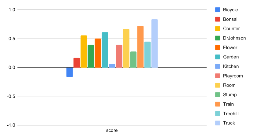
Figure 11. Average per-scene user study score. A positive score indicates a preference for our method, whereas a negative score indicates a preference for 3DGS.

Appendix E Per-Scene Quality Metrics

We provide per-scene results for Mip-NeRF 360 (Barron et al., 2022), Tanks & Temples (Knapitsch et al., 2017) and Deep Blending (Hedman et al., 2018) in Tabs. 5 and 6. Results with dagger ($\dagger$) were reproduced from Kerbl et al. (2023). We evaluate our final hierarchical rasterizer (“Ours”), as well as the fixed-size head sorting method for two different resorting window sizes (“Head 8” and “Head 16”). Additionally, we compare these methods with and without per-tile depth (“w/o PTD”).

Appendix F Per-Scene Performance Timings

In Tab. 7, we show per-scene performance timings for the total render time in ms. For the Mip-NeRF 360 (Barron et al., 2022) Indoor and Outdoor scenes, our method is slightly slower than 3DGS. For the Tanks & Temples (Knapitsch et al., 2017) and Deep Blending (Hedman et al., 2018) datasets, we achieve higher performance than 3DGS for most scenes. Analyzing the performance in more detail, we could verify that our method outperforms 3DGS when Gaussian are larger and/or more anisotropic, as our culling and load balancing can speed up rendering. If Gaussians are small and uniformly sized, the main load stems from the final stages of the render kernel, where sorting of course creates an overhead compared to 3DGS.

Table 5. Combined PSNR, SSIM, LPIPS (Zhang et al., 2018) and F LIP (Andersson et al., 2020) scores for the Mip-NeRF 360 dataset.

Dataset	Mip-NeRF 360 Outdoor					Mip-NeRF 360 Indoor
Scene	Bicycle	Flowers	Garden	Stump	Treehill	Room	Counter	Kitchen	Bonsai
PSNR$\uparrow$
Barron et al. (2022)$\dagger$	24.30	21.65	26.88	26.36	22.93	31.47	29.45	31.99	33.40
Müller et al. (2022)$\dagger$ (base)	22.19	20.35	24.60	23.63	22.36	29.27	26.44	28.55	30.34
Müller et al. (2022)$\dagger$ (big)	22.17	20.65	25.07	23.47	22.37	29.69	26.69	29.48	30.69
Fridovich-Keil et al. (2022)$\dagger$	21.90	20.10	23.50	20.68	22.26	27.57	23.64	23.43	24.71
3DGS	25.18	21.48	27.24	26.62	22.45	31.49	28.98	31.35	32.10
Head 8 w/o PTD	25.18	21.49	27.14	26.64	22.41	30.77	28.83	31.06	31.85
Head 8	25.19	21.50	27.20	26.62	22.52	30.88	28.78	31.04	31.98
Head 16 w/o PTD	25.20	21.48	27.18	26.62	22.45	30.84	28.84	30.89	31.63
Head 16	25.22	21.55	27.12	26.59	22.50	30.81	28.78	31.06	31.88
Ours w/o PTD	25.21	21.45	27.17	26.68	22.47	30.84	28.70	31.23	31.90
Ours	25.20	21.50	27.16	26.69	22.43	30.83	28.59	31.13	31.93
3DGS (Opacity Decay)	24.93	21.30	27.05	26.57	22.39	31.03	28.64	31.07	31.52
Ours (Opacity Decay)	25.00	21.30	26.95	26.67	22.39	30.58	28.33	30.46	30.76
SSIM$\uparrow$
Barron et al. (2022)$\dagger$	0.685	0.584	0.809	0.745	0.631	0.910	0.892	0.917	0.938
Müller et al. (2022)$\dagger$ (base)	0.491	0.450	0.649	0.574	0.518	0.855	0.798	0.818	0.890
Müller et al. (2022)$\dagger$ (big)	0.512	0.486	0.701	0.594	0.542	0.871	0.817	0.858	0.906
Fridovich-Keil et al. (2022)$\dagger$	0.495	0.432	0.606	0.523	0.510	0.840	0.758	0.648	0.814
3DGS	0.763	0.603	0.862	0.772	0.632	0.917	0.906	0.925	0.939
Head 8 w/o PTD	0.766	0.602	0.862	0.773	0.633	0.917	0.905	0.925	0.939
Head 8	0.766	0.604	0.862	0.773	0.634	0.916	0.905	0.924	0.939
Head 16 w/o PTD	0.767	0.603	0.861	0.773	0.633	0.917	0.905	0.922	0.939
Head 16	0.767	0.604	0.861	0.773	0.635	0.917	0.905	0.925	0.939
Ours w/o PTD	0.767	0.603	0.862	0.775	0.635	0.917	0.904	0.925	0.939
Ours	0.767	0.604	0.862	0.775	0.635	0.917	0.903	0.925	0.939
3DGS (Opacity Decay)	0.749	0.592	0.854	0.770	0.626	0.914	0.899	0.921	0.937
Ours (Opacity Decay)	0.756	0.593	0.855	0.775	0.629	0.914	0.898	0.920	0.935
LPIPS$\downarrow$
Barron et al. (2022)$\dagger$	0.305	0.346	0.171	0.261	0.347	0.213	0.207	0.128	0.179
Müller et al. (2022)$\dagger$ (base)	0.487	0.481	0.312	0.450	0.489	0.301	0.342	0.254	0.227
Müller et al. (2022)$\dagger$ (big)	0.446	0.441	0.257	0.421	0.450	0.261	0.306	0.205	0.193
Fridovich-Keil et al. (2022)$\dagger$	0.490	0.506	0.374	0.468	0.495	0.344	0.378	0.404	0.336
3DGS	0.213	0.338	0.109	0.216	0.327	0.221	0.202	0.127	0.206
Head 8 w/o PTD	0.207	0.336	0.107	0.211	0.322	0.216	0.199	0.126	0.203
Head 8	0.207	0.335	0.107	0.211	0.320	0.217	0.199	0.126	0.202
Head 16 w/o PTD	0.206	0.336	0.107	0.211	0.321	0.216	0.198	0.128	0.203
Head 16	0.206	0.335	0.107	0.211	0.319	0.216	0.199	0.126	0.202
Ours w/o PTD	0.205	0.335	0.107	0.210	0.319	0.216	0.199	0.126	0.203
Ours	0.206	0.335	0.107	0.210	0.319	0.216	0.200	0.126	0.202
3DGS (Opacity Decay)	0.244	0.358	0.125	0.232	0.347	0.230	0.215	0.137	0.210
Ours (Opacity Decay)	0.232	0.354	0.122	0.224	0.336	0.224	0.211	0.135	0.207
F LIP $\downarrow$
Barron et al. (2022)$\dagger$	0.169	0.217	0.124	0.156	0.184	0.095	0.100	0.088	0.069
Müller et al. (2022)$\dagger$ (base)	0.203	0.260	0.155	0.209	0.189	0.118	0.144	0.123	0.093
Müller et al. (2022)$\dagger$ (big)	0.201	0.251	0.146	0.213	0.189	0.112	0.139	0.113	0.089
Fridovich-Keil et al. (2022)$\dagger$	0.211	0.271	0.181	0.276	0.206	0.143	0.201	0.218	0.165
3DGS	0.158	0.225	0.118	0.150	0.186	0.093	0.105	0.096	0.082
Head 8 w/o PTD	0.160	0.223	0.120	0.150	0.184	0.102	0.107	0.100	0.086
Head 8	0.159	0.223	0.119	0.150	0.181	0.101	0.108	0.099	0.083
Head 16 w/o PTD	0.159	0.224	0.119	0.151	0.182	0.101	0.107	0.103	0.086
Head 16	0.159	0.222	0.121	0.151	0.183	0.102	0.108	0.099	0.085
Ours w/o PTD	0.160	0.225	0.120	0.149	0.183	0.101	0.110	0.099	0.085
Ours	0.159	0.224	0.119	0.149	0.184	0.101	0.111	0.099	0.084
3DGS (Opacity Decay)	0.162	0.228	0.120	0.151	0.182	0.096	0.107	0.099	0.085
Ours (Opacity Decay)	0.162	0.228	0.122	0.148	0.182	0.103	0.112	0.106	0.090

Table 6. Combined PSNR, SSIM, LPIPS (Zhang et al., 2018) and F LIP (Andersson et al., 2020) scores for Tanks & Temples and Deep Blending.

Dataset	Tanks & Temples		Deep Blending		Tanks & Temples		Deep Blending
Scene	Truck	Train	DrJohnson	Playroom	Truck	Train	DrJohnson	Playroom
Metric	PSNR$\uparrow$				SSIM$\uparrow$
Barron et al. (2022)$\dagger$	24.91	19.52	29.14	29.66	0.857	0.660	0.901	0.900
Müller et al. (2022)$\dagger$ (base)	23.26	20.17	27.75	19.48	0.779	0.666	0.839	0.754
Müller et al. (2022)$\dagger$ (big)	23.38	20.46	28.26	21.67	0.800	0.689	0.854	0.780
Fridovich-Keil et al. (2022)$\dagger$	23.23	18.94	23.16	23.02	0.774	0.663	0.787	0.802
3DGS	25.39	22.04	29.06	29.86	0.878	0.813	0.898	0.901
Head 8 w/o PTD	24.79	21.52	29.40	30.29	0.877	0.809	0.902	0.905
Head 8	24.81	21.41	29.51	30.31	0.878	0.810	0.904	0.905
Head 16 w/o PTD	24.84	21.60	29.40	30.36	0.878	0.810	0.904	0.905
Head 16	24.81	21.36	29.44	30.31	0.877	0.809	0.903	0.906
Ours w/o PTD	24.93	21.53	29.44	30.31	0.878	0.810	0.903	0.905
Ours	24.93	21.48	29.42	30.31	0.878	0.808	0.903	0.905
3DGS (Opacity Decay)	25.31	21.73	28.18	29.69	0.874	0.804	0.888	0.899
Ours (Opacity Decay)	24.90	21.46	29.38	30.30	0.875	0.804	0.903	0.907
Metric	LPIPS$\downarrow$				F LIP $\downarrow$
Barron et al. (2022)$\dagger$	0.159	0.354	0.237	0.252	0.162	0.302	0.117	0.158
Müller et al. (2022)$\dagger$ (base)	0.274	0.386	0.381	0.465	0.194	0.297	0.141	0.375
Müller et al. (2022)$\dagger$ (big)	0.249	0.360	0.352	0.428	0.190	0.291	0.133	0.311
Fridovich-Keil et al. (2022)$\dagger$	0.308	0.379	0.433	0.418	0.196	0.328	0.222	0.266
3DGS	0.148	0.208	0.247	0.246	0.148	0.250	0.119	0.143
Head 8 w/o PTD	0.143	0.204	0.236	0.237	0.165	0.265	0.116	0.140
Head 8	0.142	0.203	0.234	0.235	0.166	0.266	0.114	0.139
Head 16 w/o PTD	0.142	0.203	0.234	0.236	0.166	0.262	0.115	0.138
Head 16	0.142	0.203	0.234	0.235	0.164	0.267	0.116	0.139
Ours w/o PTD	0.142	0.204	0.234	0.235	0.163	0.264	0.115	0.139
Ours	0.142	0.204	0.234	0.235	0.164	0.267	0.115	0.138
3DGS (Opacity Decay)	0.160	0.228	0.265	0.260	0.148	0.261	0.124	0.144
Ours (Opacity Decay)	0.151	0.218	0.241	0.241	0.160	0.267	0.115	0.138

Table 7. Total performance timings for different configurations of our method and 3DGS, with the respective number of Gaussians per scene for comparison. Times in ms for FullHD resolution, averaged over 4 runs with an interpolated camera path between all available COLMAP poses (30 frames per pose).

Scene	Bicycle	Flowers	Garden	Stump	Treehill
#Gaussians	5.95M	3.60M	5.49M	4.84M	3.85M
(A) Ours	6.829	4.921	7.247	4.693	5.012
(B) Ours w/o per-tile depth	6.730	4.693	7.160	4.509	4.879
(C) Ours w/o load balancing	8.482	6.732	9.167	6.496	6.919
(D) Ours w/o tile-based culling	10.066	7.338	9.796	6.584	7.884
(E) Ours w/o hier. culling	11.087	7.589	11.788	7.178	7.773
3DGS	7.438	4.002	6.034	3.708	4.492
Scene		Bonsai	Counter	Kitchen	Room
#Gaussians		1.25M	1.20M	1.81M	1.55M
(A) Ours		3.399	4.390	5.695	3.990
(B) Ours w/o per-tile depth		3.285	4.250	5.587	3.844
(C) Ours w/o load balancing		5.251	6.217	7.558	5.843
(D) Ours w/o tile-based culling		4.846	6.977	8.214	6.155
(E) Ours w/o hier. culling		4.608	6.142	8.916	5.450
3DGS		2.574	4.043	4.783	4.180
Dataset		Deep Blending		Tanks & Temples
Scene		DrJohnson	Playroom	Train	Truck
#Gaussians		3.28M	2.33M	1.05M	2.56M
(A) Ours		4.763	4.549	4.225	5.100
(B) Ours w/o per-tile depth		4.612	4.373	4.099	4.898
(C) Ours w/o load balancing		6.648	6.275	6.215	6.942
(D) Ours w/o tile-based culling		7.998	7.295	7.469	8.363
(E) Ours w/o hier. culling		6.418	5.999	5.675	7.113
3DGS		5.752	4.303	5.548	5.506

References

- (1)
- Andersson et al. (2020) Pontus Andersson, Jim Nilsson, Tomas Akenine-Möller, Magnus Oskarsson, Kalle Åström, and Mark D. Fairchild. 2020. FLIP: A Difference Evaluator for Alternating Images. Proceedings of the ACM on Computer Graphics and Interactive Techniques 3, 2, Article 15 (2020), 23 pages.
- Barron et al. (2021) Jonathan T. Barron, Ben Mildenhall, Matthew Tancik, Peter Hedman, Ricardo Martin-Brualla, and Pratul P. Srinivasan. 2021. Mip-NeRF: A Multiscale Representation for Anti-Aliasing Neural Radiance Fields. In International Conference on Computer Vision.
- Barron et al. (2022) Jonathan T. Barron, Ben Mildenhall, Dor Verbin, Pratul P. Srinivasan, and Peter Hedman. 2022. Mip-NeRF 360: Unbounded Anti-Aliased Neural Radiance Fields. In IEEE/CVF Conference on Computer Vision and Pattern Recognition.
- Barron et al. (2023) Jonathan T. Barron, Ben Mildenhall, Dor Verbin, Pratul P. Srinivasan, and Peter Hedman. 2023. Zip-NeRF: Anti-Aliased Grid-Based Neural Radiance Fields. In International Conference on Computer Vision.
- Batcher (1968) Kenneth E. Batcher. 1968. Sorting Networks and Their Applications. In Proceedings of the Spring Joint Computer Conference.
- Broxton et al. (2020) Michael Broxton, John Flynn, Ryan Overbeck, Daniel Erickson, Peter Hedman, Matthew DuVall, Jason Dourgarian, Jay Busch, Matt Whalen, and Paul Debevec. 2020. Immersive Light Field Video with a Layered Mesh Representation. ACM Transactions on Graphics 39, 4, Article 86 (2020), 15 pages.
- Butler et al. (2012) Daniel J. Butler, Jonas Wulff, Garrett B. Stanley, and Michael J. Black. 2012. A Naturalistic Open Source Movie for Optical Flow Evaluation. In European Conference on Computer Vision.
- Chen et al. (2022) Anpei Chen, Zexiang Xu, Andreas Geiger, Jingyi Yu, and Hao Su. 2022. TensoRF: Tensorial Radiance Fields. In European Conference on Computer Vision.
- Chen et al. (2023) Yiwen Chen, Zilong Chen, Chi Zhang, Feng Wang, Xiaofeng Yang, Yikai Wang, Zhongang Cai, Lei Yang, Huaping Liu, and Guosheng Lin. 2023. GaussianEditor: Swift and Controllable 3D Editing with Gaussian Splatting. arXiv preprint arXiv:2311.14521 (2023).
- Eldridge et al. (2000) Matthew Eldridge, Homan Igehy, and Pat Hanrahan. 2000. Pomegranate: A Fully Scalable Graphics Architecture. In SIGGRAPH.
- Fang et al. (2023) Jiemin Fang, Junjie Wang, Xiaopeng Zhang, Lingxi Xie, and Qi Tian. 2023. GaussianEditor: Editing 3D Gaussians Delicately with Text Instructions. arXiv preprint arXiv:2311.16037 (2023).