Time-Modulated Arrays with Haar Wavelets

Abstract

Time-modulated arrays (TMAs) can effectively perform beamsteering over the first positive harmonic pattern by applying progressively delayed versions of stair-step approximations of a sine waveform to the antenna excitations. In this letter, we consider synthesizing such stair-step sine approximations by means of Haar wavelets. Haar functions constitute a complete orthonormal set of rectangular waveforms which have the ability to represent a given function with a high degree of accuracy using few constituent terms. Hence, when they are applied to TMA synthesis, employing single-pole double-throw switches, such a feature leads to an excellent rejection level of the undesired harmonics as well as a bandwidth greater than that supported by conventional TMAs with on-off switches.

I Introduction

Time-modulated arrays (TMA) have the ability to perform beamsteering (BS) by adjusting the on-off instants of the switches that constitute their feeding network. They can be considered as a cost-effective alternative for smart antennas solutions that does not require variable phase shifters. time-modulated array (TMA) designs, however, have some handicaps such as the control of the unexploited harmonics [1, 2], the presence of mirrored frequency diagrams [3, 4], the transmitted (and received) signal energy wasted during the zero-state of the switches [5, 6], and the allowable signal bandwidth due to the spectral overlapping with the signal replicas [7, 8]. When designing TMAs for BS purposes, the aforementioned drawbacks can be alleviated by means of:

1. The use of stair-step approximations of time-delayed sine functions –with fundamental frequency $\omega_{0}$– as the TMA modulating waveforms. This significantly decreases the level of the unexploited sideband radiation (SR). Stair-step approximations also avoid the energy-absorbing zero-state of the conventional on-off switches and are easily implementable with single-pole double-throw (SPDT) switches [9, 10].

2. The use of single sideband (SSB) (or complex) TMA architectures capable of suppressing power-consuming frequency-mirrored harmonic patterns [4, 11], even using amplitude-phase weighting with multiple branches [7].

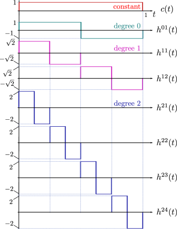
Figure 1: The first eight Haar wavelets $h^{lm}(t)$ with degree $l=\{0,1,2\}$ and order $m=1,\dots,2^{l}$.

In this letter we will follow a different approach. The approximated time-delayed sine waveforms which modulate the individual TMA elements will be synthesized by means of a complete set of orthogonal functions: the Haar wavelets [12, 13]. As shown in Section II, a Haar wavelet $h^{lm}(t)$ is characterized by its degree $l$ and order $m$. Haar wavelets with the same degree $l>0$ are successive time-multiplexed (non overlapped) versions of the corresponding $m=1$ first-order wavelet (see Fig. 1). Hence, Haar wavelets are well suited for TMA synthesis because those with the same degree can be easily generated employing SPDT switches, thus enabling a significant complexity reduction.

Accordingly, a given function can be expressed as a linear combination of Haar wavelets whose coefficients are obtained solving integrals similar to those of the Fourier series coefficients, but using the corresponding Haar wavelet instead of sines or cosines. Furthermore, analogously to the discrete Fourier Transform (DFT), the Haar Discrete Wavelet Transform (HDWT) can be used to efficiently compute the Haar coefficients. Indeed, since Haar wavelets may be written in matrix notation by a Haar matrix, when a vector with samples of the waveform to be approximated is given, the calculation of the Haar coefficients is performed by just a matrix product.

The main contribution of this letter is the application of Haar wavelets to the design of TMA modulating waveforms to perform beamsteering over the first positive harmonic pattern.

II Haar Wavelets

Except for the special case $c(t)=1$ for $0\leq t\leq 1$ (a constant unitary function), Haar wavelets are defined as follows

$$h^{lm}(t)=\begin{cases}\sqrt{2^{l}}&\frac{m-1}{2^{l}}\leq t\leq\frac{m-\frac{1}{2}}{2^{l}}\\ -\sqrt{2^{l}}&\frac{m-\frac{1}{2}}{2^{l}}<t\leq\frac{m}{2^{l}}\\ 0&\text{otherwise}\end{cases},$$ (1)

being $l=0,1,2,\dots$ and $m=1,\dots,2^{l}$. The degree $l$ denotes a subset having the same number of zero crossings in a given width, ${1}/{2^{l}}$, and the order $m$ gives the position of the function within this subset. All the members of a subset with the same degree are obtained by shifting the first member along the axis by an amount proportional to its order (see Fig. 1).

A given continuous function, $f(t)$, within the interval $0\leq t\leq 1$ and repeated periodically outside this interval, can be synthesized from a Haar series as follows [12]:

$$f(t)=W^{0}+\sum_{l=0}^{\infty}\sum_{m=1}^{2^{l}}W^{lm}h^{lm}(t)=W^{0}+\sum_{l=0}^{\infty}\mathop{\mathcal{H}}\nolimits^{l}(t)$$ (2)

and, by virtue of the orthonormality between Haar wavelets, we have that the corresponding Haar wavelet coefficients are

$$W^{0}=\int_{0}^{1}f(t)dt\text{ and }W^{lm}=\int_{0}^{1}f(t)h^{lm}(t)dt,$$ (3)

satisfying the extremal of the squared error integral condition

$$\lim_{\Gamma\to\infty}\int_{0}^{1}\left|f(t)-\left(W^{0}+\sum_{l=0}^{\Gamma}\mathop{\mathcal{H}}\nolimits^{l}(t)\right)\right|^{2}dt=0.$$ (4)

If the series expansion in Eq. 2 is truncated at $l=\Gamma$, a finite set of Haar wavelets is considered for the synthesis and a stair-step approximation of $f(t)$ is obtained. Furthermore, the HDWT can be interpreted as the mathematical operator that converts a finite sequence of equally-spaced samples of $f(t)$ into a sequence (with the same length) of Haar wavelet coefficients. For numerical handling, we consider a discrete series of $M=2^{p}$ terms (with $p\in\mathbb{N}$) obtained by sampling $f(t)$ at $M$ equally spaced points $x_{k}$ over $[0,1)$, with $k\in\Psi=\{1,2,\dots,M\}$. Hence, the integrals in Eq. 3 can be replaced by the finite sums:

$$W^{0}=\frac{1}{M}\sum_{k=1}^{M}f(x_{k})\text{ and }W^{lm}=\frac{1}{M}\sum_{k=1}^{M}f(x_{k})h^{lm}(x_{k}),$$ (5)

with $l\in\Lambda=\{0,\dots,p-1\}$ and $m\in\Xi=\{1,\dots,2^{l}\}$. The resulting values for $\{W^{0},W^{lm}\}$ constitute the HDWT of $f(t)$. Notice that the HDWT can be recursively described by a real-valued square matrix considering the Kronecker product (denoted as $\otimes$) as follows:

$$H_{M}=\frac{1}{\sqrt{2}}\begin{bmatrix}H_{M/2}&\otimes&\begin{pmatrix}+1&+1\end{pmatrix}\\ I_{M/2}&\otimes&\begin{pmatrix}+1&-1\end{pmatrix}\end{bmatrix},$$ (6)

being $(+1+1)$ and $(+1-1)$ row vectors, and $I_{M/2}$ the identity matrix of order $M/2$. The iteration starts with $H_{1}=[1]$, and we easily realize that the first $M$ Haar wavelets (see Fig. 1) –or rather, samples of such wavelets– are the rows of $H_{M}$. Hence, by considering $f(t)$ in $[0,T_{0})$, with normalized period $T_{0}=1$, we can arrange $M=2^{p}$ equally spaced samples of $f(t)$ in a column vector $\bar{f}_{M}=[f(x_{1}),\dots,f(x_{M})]^{T}$ and represent –by virtue of Eq. 5– the corresponding HDWT of $f(t)$ through the following matrix equation:

$$\overline{W}_{M}{=}[W^{0}W^{01}W^{11}W^{12}\cdots W^{(p-1)2^{p-1}}]{=}\frac{1}{M}H_{M}\cdot\overline{f}_{M},$$ (7)

being $\overline{W}_{M}$ a column vector with the Haar-wavelet coefficients in Eq. 5, and $H_{M}$ the HDWT matrix in Eq. 6 with order $M$.

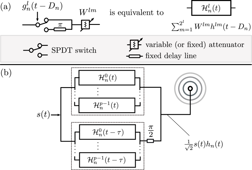
Figure 2: (a) SPDT switching architecture capable of generating the term $\sum_{m=1}^{2^{l}}W^{lm}h^{lm}(t)$ in Section III for a given Haar wavelet of degree $l$. Notice that $g_{n}^{l}(t-D_{n})$ is a square wave with frequency $2^{l}f_{0}$ subject to a time delay $D_{n}$, whereas $\mathop{\mathcal{H}}\nolimits_{n}^{l}(t)=\sum_{m=1}^{2^{l}}W^{lm}h^{lm}(t-D_{n})$. The Haar coefficients $W^{lm}$ are implemented with either a variable or a fixed (depending on $l$) attenuator. (b) Generalized architecture for the $n$-th TMA element feeding network which synthesizes a Haar wavelet. Note that for the entire array, $N$ time-modulators like this one are needed (plus a $1{:}N$ splitter).

III Time-varying array factor controlled by Haar wavelets

We propose to apply Haar synthesis to design TMAs with BS capabilities. The idea is to approximate the functions employed for time-modulating the TMA excitations (sine waveforms) by means of linear combinations of Haar wavelets (easily implemented with SPDT switches and variable attenuators). Hence, the time-varying array factor is expressed as a function of the Haar coefficients of such functions.

Fig. 2 shows the proposed feeding architecture for the $n$-th element of a linear TMA with $N$ isotropic elements ($n\in\Theta=\{0,\dots,N-1\}$) requiring only SPDT switches, VAs, and fixed delay lines. In such a feeding network, the excitation of the $n$-th antenna element is time-modulated by the periodic ($T_{0}$) pulse $h_{n}(t)=h(t-D_{n})$, being $h(t)=f(t)+\mathrm{j}f(t-\tau)$, where $f(t)$ is an approximation of a sine waveform with fundamental frequency $\omega_{0}=2\pi f_{0}=2\pi/T_{0}$, $\mathrm{j}$ is the imaginary unit, and $D_{n}$ and $\tau$ are adaptive and fixed (defined beforehand) time delays, respectively.

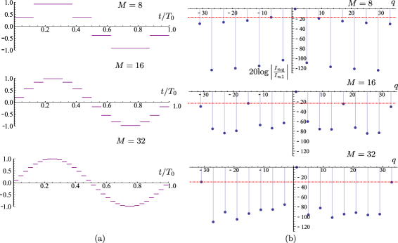
Figure 3: (a) Stair-step approximations of $\sin(2\pi t)$ considering the HDWT with $M=8$, $16$, and $32$ equally spaced points. (b) Relative power level of the dynamic excitations of the unexploited harmonics. Table II shows the values of the peak SR and the maximum signal bandwidth $B_{\text{max}}$.

TABLE I: Time-varying Haar BFNs for each value of $M$ when a sine waveform is synthesized.

	$\mathop{\mathcal{H}}\nolimits^{0}(t)$	$\mathop{\mathcal{H}}\nolimits^{2}(t)$	$\mathop{\mathcal{H}}\nolimits^{3}(t)$	$\mathop{\mathcal{H}}\nolimits^{4}(t)$
$M=8$	yes	yes	no	no
$M=16$	yes	yes	yes	no
$M=32$	yes	yes	yes	yes
Type of attenuator	none	fixed	VA	VA
Discrete levels (dB)	0	-13.6	-20.0,-27.7	-28.5,-29.9,-33.4,-42.5

TABLE II: Performance comparison between SSB switched TMAs.

Reference	Peak SR (dB)	$B_{\text{max}}$ (Hz)	$\eta_{\text{TMA}}$(%)	$\eta_{\text{mod}}$(%)	$\eta$(%)
[7]	-25.00	8$f_{0}$	97.90	20.70	20.27
[4]	-13.98	4$f_{0}$	91.19	33.33	30.40
[14]	-16.90	8$f_{0}$	94.96	50.00	47.48
[9]	-16.90	8$f_{0}$	96.00	58.00	55.68
[10]	-23.50	16$f_{0}$	98.72	50.00	49.36
Proposed ($M$=32)	-29.80	32$f_{0}$	99.68	50.00	49.84

In the synthesis of $f(t)$ in Eq. 2, we realize that $W^{0}=0$ because $f(t)$ is an approximation of a pure sine (without direct-current component) and $h^{lm}(t)$ is a periodic ($T_{0}$) Haar wavelet whose Fourier series expansion is given by $h^{lm}(t)=\sum_{q=-\infty}^{\infty}G_{q}^{lm}\mathrm{e}^{\mathrm{j}q\omega_{0}t}$, being $G_{q}^{lm}$ the corresponding Fourier coefficients. By substituting the previous equation into Eq. 2 we have

$$f(t) =\sum_{l=0}^{p-1}\sum_{m=1}^{2^{l}}W^{lm}h^{lm}(t)$$

$$=\sum_{q=-\infty}^{\infty}\left[\sum_{l=0}^{p-1}\sum_{m=1}^{2^{l}}W^{lm}G_{q}^{lm}\right]\mathrm{e}^{\mathrm{j}q\omega_{0}t}.$$ (8)

If we select a delay $\tau$ verifying $\omega_{0}\tau=\pi/2$, then $\mathrm{e}^{-\mathrm{j}q\omega_{0}\tau}=(-\mathrm{j})^{q}$ and, applying the time-shifting property to the Fourier coefficients in Section III, we write $h(t)=f(t)+\mathrm{j}f(t-\tau)$ as

$$h(t)=\sum_{q=-\infty}^{\infty}[1-(-\mathrm{j})^{q+1}]\left[\sum_{l=0}^{p-1}\sum_{m=1}^{2^{l}}W^{lm}G_{q}^{lm}\right]\mathrm{e}^{\mathrm{j}q\omega_{0}t},$$ (9)

and by applying again the time-shifting property to the Fourier coefficients, we express $h_{n}(t)=h(t-D_{n})$ as

$$h_{n}(t){=}\sum_{q=-\infty}^{\infty}[1-({-}\mathrm{j})^{q+1}]\left[\sum_{l=0}^{p-1}\sum_{m=1}^{2^{l}}W^{lm}G_{q}^{lm}\right]\mathrm{e}^{-\mathrm{j}q\omega_{0}D_{n}}\mathrm{e}^{\mathrm{j}q\omega_{0}t}.$$ (10)

Therefore, the TMA element architecture shown in Fig. 2 leads to the following time-varying array factor (with the term $\mathrm{e}^{\mathrm{j}\omega_{c}t}$ explicitly included) as a function of the coefficients of the modulating Haar wavelets:

$$F(\theta,t)=\frac{\mathrm{e}^{\mathrm{j}q\omega_{c}t}}{\sqrt{2}}\sum_{n=0}^{N-1}h_{n}(t)\mathrm{e}^{\mathrm{j}kz_{n}\cos\theta}$$

$$=\sum_{q=-\infty}^{\infty}\sum_{n=0}^{N-1}\left[\sum_{l=0}^{p-1}\sum_{m=1}^{2^{l}}\frac{1-(-\mathrm{j})^{q+1}}{\sqrt{2}}W^{lm}G_{q}^{lm}\cdot\right.$$

$$\cdot\mathrm{e}^{-\mathrm{j}q\omega_{0}D_{n}}\mathrm{e}^{\mathrm{j}kz_{n}\cos\theta}\Bigg{]}\mathrm{e}^{\mathrm{j}(\omega_{c}+q\omega_{0})t}=\sum_{q=-\infty}^{\infty}F_{q}(\theta)\mathrm{e}^{\mathrm{j}(\omega_{c}+q\omega_{0})t},$$ (11)

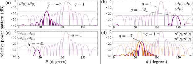
Figure 4: (a), (b), and (c): Power radiated patterns of single-beam TMAs designed with Haar wavelets for $M=8$, $16$, and $32$ (Haar feeding networks employed are explicitly indicated). Notice that the phase excitations are considered to be progressive, i.e., the useful harmonic beam points to the direction $\theta_{0}$ (in the example, $\theta_{0}=110^{\circ}$) when $\omega_{0}D_{n}=\pi n\cos(\theta_{0})$, $n\in\Theta$ (see Eq. 12). (d) An advantage of the technique in terms of flexibility is that the single beam architecture employed for $M=32$ can be exploited to generate two independent beams with the features corresponding to $M=8$.

where $z_{n}$ represents the $n$-th array element position on the $z$ axis, $\theta$ is the angle with respect to such a main axis, and $k=2\pi/\lambda_{c}$ represents the wavenumber for a wavelength $\lambda_{c}=2\pi\mathrm{c}/\omega_{c}$, with $\omega_{c}$ being the carrier frequency and $\mathrm{c}$ the speed of light. Notice that $F_{q}(\theta)=\sum_{n=0}^{N-1}I_{nq}\mathrm{e}^{\mathrm{j}kz_{n}\cos\theta}$ is the spatial array factor at the frequency $\omega_{c}+q\omega_{0}$ and

$$I_{nq}=\sum_{l=0}^{p-1}\sum_{m=1}^{2^{l}}\frac{1-(-\mathrm{j})^{q+1}}{\sqrt{2}}W^{lm}G_{q}^{lm}\mathrm{e}^{-\mathrm{j}q\omega_{0}D_{n}},\ n\in\Theta,$$ (12)

the corresponding dynamic excitations that synthesize the radiated pattern at such a frequency. As in [11], note that

$$1-(-\mathrm{j})^{q+1}=\{2\ q\in\Upsilon;0\ \text{otherwise}\},$$ (13)

with $\Upsilon=\{q=4k-3;k\in\mathbb{Z}\}=\{\dots,-7,-3,1,5,9,\dots\}$ and the frequency-mirrored unwanted harmonics are removed (SSB feature). Hence, for a given harmonic pattern of order $q$, the corresponding dynamic excitations $I_{nq}$ in Eq. 12 have identical modulus, but they can be endowed with progressive phases for $n\in\Theta$ by selecting $D_{n}$ with the aim of performing BS. The different $D_{n}$ are easily implemented by means of the switch-on time of the individual Haar wavelets.

IV Numerical simulations

We consider a TMA with $N=16$ elements spaced $\lambda_{c}/2$ and the discrete Haar wavelet synthesis of Eq. 7 applied to $f(t)=\sin(2\pi t/T_{0})$ for the cases of $M=8$, $16$, and $32$ equally spaced points in the interval $(0,2\pi]$. As indicated above, we assume a normalized period $T_{0}=1$. Fig. 3 illustrates the synthesized stair-step approximations of $f(t)$ and the corresponding relative power level of the dynamic excitations (having identical modulus for $n\in\Theta$) of the unexploited harmonics with respect to the dynamic excitation levels of the useful harmonic at $q=1$.

Table I shows the Haar beamforming networks needed for each value of $M$ and the characteristics of the attenuators. $\mathop{\mathcal{H}}\nolimits^{0}(t)$ does not require attenuation ($W^{lm}=1$ in Fig. 2a), $\mathop{\mathcal{H}}\nolimits^{2}(t)$ employs a fixed attenuator of $-13.6$ dB, whereas $\mathop{\mathcal{H}}\nolimits^{3}(t)$ and $\mathop{\mathcal{H}}\nolimits^{4}(t)$ require VAs with $2$ and $4$ discrete levels, respectively, which are specified in Table I. Table II illustrates the peak SR, the maximum signal bandwith ($B_{\text{max}}$), and the efficiencies of the time modulation method [11]: $\eta_{\text{TMA}}$, which accounts for the ability of the TMA to filter out and radiate only the useful harmonics; $\eta_{\text{mod}}$, which accounts for the reduction of the total mean power radiated by a uniform static array caused by the insertion of the TMA switched feeding network; and $\eta=\eta_{\text{TMA}}\cdot\eta_{\text{mod}}$, which represents the total TMA efficiency. The improvement of the peak SR and the $B_{\text{max}}$ for $M=16$ (39% and 100%, respectively) and $M=32$ (76% and 300%, respectively) when compared to that of [14], is remarkable. Additionally, we point out that a key difference between [10] and this technique is that Walsh functions occupy an entire period (since they are not time multiplexed like Haar wavelets with the same degree). Hence, each Walsh function must be synthesized by an independent switch, thus increasing the complexity to achieve the same performance.

Fig. 4a to Fig. 4c show the power radiated patterns and the Haar feeding networks employed for three different values of $M$. These figures evidence the outstanding rejection level of the unwanted harmonics. Fig. 4d shows that we can exploit the scheme used for $M=32$ to generate two independent beams. Notice that with feeding networks $\mathop{\mathcal{H}}\nolimits^{3}(t)$ and $\mathop{\mathcal{H}}\nolimits^{4}(t)$ (see Fig. 2a) we can implement $\mathop{\mathcal{H}}\nolimits^{0}(t)$ and $\mathop{\mathcal{H}}\nolimits^{2}(t)$ by modifying the frequency of $g_{n}^{l}(t-D_{n})$ and the attenuations $W^{lm}$, and governing these two networks by means of square waves with frequencies different than $f_{0}$ and $4f_{0}$, respectively.

It is remarkable that a $b$-bit digital phase shifter, a core element of standard phased arrays, is usually constituted by $2b$ cascaded SPDT switches [15], and when $b$ increases, so does both the phase resolution and the insertion losses. With the proposed technique, the phase resolution is independent of the number of switches and, with $2b$ SPDT switches, we can implement a Haar BFN of order $M=2^{b+1}$. Since $M$ increases with $b$, the total insertion losses of the Haar BFN will decrease with $b$ (see $\eta$ values in Table II).

V Conclusions

We proposed a novel approach to TMA beamsteering based on HDWT modulation. Compared to existing switched TMAs, the method provides better rejection of the undesired harmonics and allows for higher signal bandwidths, although at the expense of a moderate increase of the hardware complexity.

References

- [1] R. Maneiro Catoira, J. Brégains, J. A. Garcia-Naya, L. Castedo, P. Rocca, and L. Poli, “Performance analysis of time-modulated arrays for the angle diversity reception of digital linear modulated signals,” IEEE J. Sel. Topics Signal Process., vol. 11, no. 2, pp. 247–258, Mar. 2017.
- [2] Y. Tong and A. Tennant, “Simultaneous control of sidelobe level and harmonic beam steering in time-modulated linear arrays,” Electronics Letters, vol. 46, no. 3, pp. 201–202, Feb. 2010.
- [3] L. Poli, P. Rocca, G. Oliveri, and A. Massa, “Harmonic beamforming in time-modulated linear arrays,” IEEE Trans. Antennas Propag., vol. 59, no. 7, pp. 2538–2545, Jul. 2011.
- [4] A. M. Yao, W. Wu, and D. G. Fang, “Single-sideband time-modulated phased array,” IEEE Trans. Antennas Propag., vol. 63, no. 5, pp. 1957–1968, May 2015.
- [5] Q. Zhu, S. Yang, R. Yao, and Z. Nie, “Gain improvement in time-modulated linear arrays using spdt switches,” IEEE Antennas Wireless Propag. Lett., vol. 11, pp. 994–997, 2012.
- [6] S. Yang, Y. Gan, and P. Tan, “Evaluation of directivity and gain for time-modulated linear antenna arrays,” Microw. Opt. Technol. Lett., vol. 42, p. 167–171, 2004.
- [7] H. Li, Y. Chen, and S. Yang, “Harmonic beamforming in antenna array with time-modulated amplitude-phase weighting technique,” IEEE Trans. Antennas Propag., vol. 67, no. 10, pp. 6461–6472, Oct. 2019.
- [8] G. Bogdan, K. Godziszewski, Y. Yashchyshyn, C. H. Kim, and S. Hyun, “Time modulated antenna array for real-time adaptation in wideband wireless systems—part I: Design and characterization,” IEEE Trans. Antennas Propag., pp. 1–9, Mar. 2019.
- [9] R. Maneiro-Catoira, J. Brégains, J. A. García-Naya, and L. Castedo, “Time-modulated array beamforming with periodic stair-step pulses,” Signal Processing, vol. 166, p. 107247, 2020.
- [10] R. Maneiro-Catoira, M. B. A. Avele, J. Brégains, J. A. García-Naya, and L. Castedo, “Beam-steering in switched 4D arrays based on the discrete Walsh transform,” in Proc. of 27th European Signal Processing Conference (EUSIPCO), Sep. 2019, pp. 1–5.
- [11] R. Maneiro-Catoira, J. Brégains, J. A. García-Naya, and L. Castedo, “Time-modulated phased array controlled with nonideal bipolar squared periodic sequences,” IEEE Antennas Wireless Propag. Lett., vol. 18, no. 2, pp. 407–411, Feb 2019.
- [12] J. R. McLaughlin, “Haar series.” Transactions of the American Mathematical Society, vol. 137, pp. 153–176, Mar. 1969.
- [13] J. Shore, “On the application of Haar functions,” IEEE Trans. Commun., vol. 21, no. 3, pp. 209–216, Mar. 1973.
- [14] Q. Chen, J. Zhang, W. Wu, and D. Fang, “Enhanced single-sideband time-modulated phased array with lower sideband level and loss,” IEEE Trans. Antennas Propag., vol. 68, no. 1, pp. 275–286, Jan. 2020.
- [15] “Analog devices,” https://www.analog.com, monolithic microwave integrated circuit (MMIC) digital phase shifters. HMC936A, HMC648A, HMC649A, HMC543A. Accessed: 2020-03-02.