On the minimum spanning tree distribution in grids

Abstract.

We study the minimum spanning tree distribution on the space of spanning trees of the $n$-by-$n$ grid for large $n$. We establish bounds on the decay rates of the probability of the most and the least probable spanning trees as $n\rightarrow\infty$.

1. Introduction

Let $G=G(n)$ denote the $n$-by-$n$ square grid graph, which has $n^{2}$ vertices, and let $\mathcal{T}(G)$ denote the set of all spanning trees of $G$. The MST (minimal spanning tree) distribution on $\mathcal{T}(G)$ assigns to each $T\in\mathcal{T}(G)$ the probability, $\text{Prob}_{\text{MST}}(T)$, that $T$ will result from the algorithm that builds a spanning tree one edge at a time with each next edge uniformly randomly selected, along the way rejecting each addition that would create a cycle. This is equivalent to applying Krusgal’s algorithm to find a minimum spanning tree of $G$ with respect to uniformly identically distributed edge weights in $[0,1]$.

One purpose of this paper is to better understand the support of the $MST$ distribution on $\mathcal{T}(G(n))$ asymptotically as $n\rightarrow\infty$. In other words, we wish to understand, in $G(n)$ for large $n$, the minimum and maximum values of $\text{Prob}_{\text{MST}}(T)$. We will prove the following.

Theorem 1.1.

For any family of spanning trees $\mathcal{F}=\{T_{n}\subset G(n)\mid n\in\mathbb{N}\}$,

$$\text{Prob}_{\text{MST}}(T_{n})\geq\sim\left(\frac{1}{4}\right)^{n^{2}}\text{ and }\text{Prob}_{\text{MST}}(T_{n})\leq\sim\left(\frac{1}{2}\right)^{n^{2}}.$$

The symbols “$\geq\sim$” and “$\leq\sim$” refer to the asymptotic growth. More precisely, the upper bound means that $\limsup\frac{\ln\left(\text{Prob}_{\text{MST}}(T_{n})\right)}{n^{2}}\leq\ln\frac{1}{2}$, and analogously for the lower bound.

The decay base, $Q(\mathcal{F})$, of the family $\mathcal{F}$ is the value such that $\text{Prob}_{\text{MST}}(T_{n})\sim Q(\mathcal{F})^{n^{2}}$; that is, $\lim\frac{\ln\left(\text{Prob}_{\text{MST}}(T_{n})\right)}{n^{2}}=\ln Q(\mathcal{F})$, provided such a value exists. The theorem says the $Q(\mathcal{F})\in\left[\frac{1}{4},\frac{1}{2}\right]$ if it exits.

To calibrate our understanding of Theorem 1.1, consider the case that $\mathcal{F}$ is “average” in the sense that each tree $T_{n}$ has the average $MST$-probability in $\mathcal{T}(G(n))$. It is well known from [24] that $|\mathcal{T}(G(n))|\sim\mathfrak{b}^{n^{2}}$, where $\mathfrak{b}$ is related to Catalan’s constant $C$ as follows:

$$\mathfrak{b}=\exp(4C/\pi)=3.2099\cdots.$$

Therefore the decay base of an average family equals $\frac{1}{\mathfrak{b}}$.

Figure 1 illustrates three families of spanning trees that we will study. For the double spiral and centipede family, only the tree in $G(7)$ is shown, but the pattern extends in the obvious way to a tree in $G(n)$ for all $n\geq 3$. The fractal family was first introduced in [2] to exemplify trees with low weight, but it will be used here to exemplify trees with high $MST$ probabilities. As indicated in the figure, each quadrant of $F_{k+1}$ is a copy of $F_{k}$, and these copies are connected in the middle by a copy of $F_{1}$.

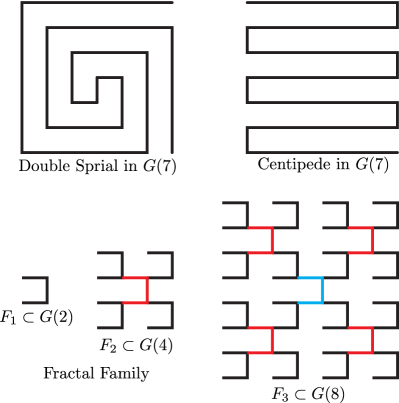
Figure 1. Three spanning tree families

This paper is organized as follows. In Section 2, we introduce a construction that associates a bipartite graph to a spanning tree. Among other things, this construction helps partially account for an empirical observation from the mathematics of redistricting, namely that spanning trees drawn from the MST distribution tend to result in more compact district maps.

In Section 3, we overview some of the literature about the average stretch and weight of a spanning tree, which correlates with the MST probability. In Section 4, we discuss the Lyons-Peres formula for the MST probability of a spanning tree, which turns out to depend only on the associated bipartite graph. Because of this, many of the propositions in this paper could be framed as results about bipartite graphs. We then prove Theorem 1.1 in Section 5.

In Section 6, we state a theorem that establishes a lower bound for the decay base of a family of spanning trees in terms of a certain power series that is naturally associated to the family. The proof of this theorem is involved and is spread through Sections 7-9. In Section 10, we study the example families of Figure 1. Finally in Section 11 we provide some conjectures and questions for further study.

2. The Bipartite Graph

In this section, we introduce a simple construction that naturally associates a bipartite graph to a spanning tree.

Let $G=(V,E)$ be a connected simple undirected graph (not necessarily a grid). Let $T$ be a spanning tree of $G$ regarded as a subset of $E$. We’ll call the edges of $T$ branches and the edges of $T^{c}=E-T$ chords. For each chord $e\in T^{c}$, let $\operatorname{Cycle}(e)$ denote the unique cycle in the graph obtained by adding $e$ to $T$. For each branch $e\in T$, let $\operatorname{Cut}(e)$ denote the cut set between the two components $T-\{e\}$; that is $\operatorname{Cut}(e)$ includes $e$ and each chord that’s incident to both components.

We define a bipartite graph $\mathcal{G}=(\mathcal{V}_{1},\mathcal{V}_{2},\mathcal{E})$ associated to the spanning tree $T$ as exemplified in Figure 2. It contains a set $\mathcal{V}_{1}$ of nodes correspond to the branches of $T$, and a set $\mathcal{V}_{2}$ of nodes corresponding to the chords, with adjacency determined by whether the branch belongs to the cycle associated to the chord. Denote $M=|\mathcal{V}_{1}|=|T|$ and $N=|\mathcal{V}_{2}|=|T^{c}|$. Notice that a branch $e\in\mathcal{V}_{1}$ is adjacent to all of the chords in $\operatorname{Cut}(e)$, while a chord $e\in\mathcal{V}_{2}$ is adjacent to all of the branches in $\operatorname{Cycle}(e)$. To avoid confusion, we’ll use the terms vertices and edges when referring to $G$, and the terms nodes and links when referring to $\mathcal{G}$.

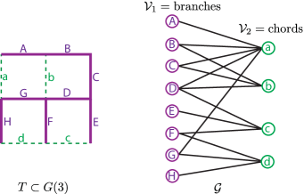
Figure 2. The bipartite graph $\mathcal{G}$ associated to a spanning tree $T\subset G(3)$

For $i\in\{1,2\}$, let $d_{i}$ denote the average degree in $\mathcal{G}$ of the nodes in $\mathcal{V}_{i}$. This paper focuses on the case where $G=G(n)$ for large $n$, in which case $M\approx N$ so $d_{1}\approx d_{2}$. In the next section we’ll overview some of the literature that studies $d_{2}$ (and slight variations of the measurement $d_{2}$ including the weight and average stretch of $T$). For now, notice that such measurements can be easily re-interpreted as reflecting the tree’s average cut-length. That is, a tree for which $d_{2}$ is small (later referred to as a tree with small weight or small average stretch) will on average form a bipartition with fewer cut edges when a random one of its branches is removed (because $d_{1}$ is small).

In the literature on the mathematics of redistricting, it has been observed empirically that a spanning tree drawn from the MST distribution has exactly this advantage compared to a spanning tree drawn uniformly – it tends to form a more compact bipartition when one of its branches is removed; see [8]. This observation is partially accounted for by the above comments together with the observation that a spanning tree with higher MST probability tends to have a lower $d_{2}$.

3. Previous results about weight and stretch

In this section, we overview some of the literature about the weight/stretch of a spanning tree $T\subset G$.

The seminal paper [2] considered the following measurement, in which $\text{dist}_{T}(e)$ denotes the path-length-distance in $T$ between the two endpoints of the edge $e\in E$ (which equals $1$ if $e\in T$):

$$\text{avg-stretch}(T)=\text{avg}\{\text{dist}_{T}(e)\mid e\in E\}=\frac{M+N\cdot d_{2}}{M+N}.$$

Adressing a conjecture from [7], they proved for a general graph $G$ with $v$ vertices, that $G$ contains a spanning tree $T$ such that

(3.1) $$\text{avg-stretch}(T)=\exp\left(\mathcal{O}\left(\log v\log\log v\right)\right),$$

and for grid graphs, they identified constants $C_{1},C_{2}$ for which

(3.2) $$C_{1}\cdot\ln(n)\leq\min\{\text{avg-stretch}(T)\mid T\in\mathcal{T}(G(n))\}\leq C_{2}\cdot\ln(n).$$

Much of the follow up literature was concerned with sharpening Equation 3.1 for general graphs [1],[3],[4],[11] and for special classes of graphs including $k$-outerplanar [10] and polygonal 2-trees [21], and with sharpening the constants $C_{1}$ and $C_{2}$ for grid graphs [13], although the optimal constants are still not known. In particular, the original choice of $C_{2}$ in [2] came from the fractal family pictured in Figure 1; follow up work improved their constant for the fractal family and also identified families of spanning trees that have even lower average-stretch than the fractal family [14],[19].

Finding a spanning tree that minimizes avg-stretch is NP-hard for a general graph $G$ [7], and is very challenging for $G(n)$ even for relatively small values of $n$. Macheto-trees like the one shown in Figure 3, which minimize the maximum degree in $\mathcal{V}_{2}$, are also avg-stretch optimizers for $G(7)$ [25] but not for $G(8)$ [13]. Optimizers are known for $G(8)$ and $G(10)$; for example, there are more than 80,000 optimizers for $G(8)$ [13].

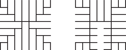
Figure 3. [from [13]] The Macheto-tree on the left doesn’t minimize avg-stretch, but the tree on the right does.

Some of the above-cited literature is reframed in terms of the following related measurement:

$$\text{weight}(T)=\sum_{e\in T^{c}}\text{length}(\operatorname{Cycle}(e))=(d_{2}+1)\cdot N.$$

For fixed $G$, $\text{avg-stretch}(T)$ and $\text{weight}(T)$ are minimized by the same $T\in\mathcal{T}(G)$, but there nevertheless are valid reasons to study the measurements separately. First, they generalize differently to weighted graphs. Second, each measurement spun off its own specific generalizations in the literature. For example, $\text{weight}(T)$ equals the weight of the fundamental cycle basis for $T$, so its generalizations include the search for spanning trees with (not necessarily fundamental) cycle bases of minimal weight [16],[17],[19],[22]. See [19] for an overview of applications including to biology, chemistry, traffic light planning, periodic railway timetabling, and electrical engineering.

On the other hand, $\text{avg-stretch}(T)$ measures the average distortion of the metric embedding of $G$ into $T$, so its generalizations include the search for a tree (not necessarily a spanning tree of $G$) or a probabilistic family of trees whose distances approximate those in $G$ with low average distortion [5],[6],[9],[11],[12],[18].

4. The Lyons-Peres Formula for $\text{Prob}_{\text{MST}}(T)$

In this section, we state and re-interpret the explicit formula for MST probability due to Lyons and Peres [23]. We will re-frame their formula in a way that makes it clear that $\text{Prob}_{\text{MST}}(T)$ depends only on the bipartite graph $\mathcal{G}$ associated to $T$.

With the assumptions and notation of Section 2, let $S(T)$ denote the set of permutations (orders) of $T$. For $\alpha=(e_{1},e_{2},\cdots,e_{M})\in S(T)$ and $1\leq i\leq M$, let $P_{i}(\alpha)$ denote the number of cut edges in the subgraph that has vertex set $V$ and edge set $\{e_{i+1},...,e_{M}\}$. Here a “cut edge” means an edge of $G(n)$ that connects two different components of the subgraph. By convention, $P_{M}(\alpha)=|E|=M+N$.

Proposition 4.1 (Lyons-Peres [23]).

$$\text{Prob}_{\text{MST}}(T)=M!\cdot\mathbb{E}\left(\frac{1}{\prod_{i=1}^{M}P_{i}(\alpha)}\right)=\sum_{\alpha\in S(T)}\frac{1}{\prod_{i=1}^{M}P_{i}(\alpha)},$$

where the $\mathbb{E}$ denotes the expectation with respect to the uniform distribution on $S(T)$.

Sketch of Proof.

The proof in [23] involves noticing that for a fixed permutation $\alpha=(e_{1},e_{2},...,e_{M})$,

$$\frac{1}{\prod_{i=1}^{M}P_{i}(\alpha)}=\frac{1}{P_{M}(\alpha)}\cdot\frac{1}{P_{M-1}(\alpha)}\cdots\frac{1}{P_{1}(\alpha)}$$

equals the probability that the algorithm described in the first paragraph of this paper will yield $T$ in the order $(e_{M},...,e_{1})$. This is because, if $\{e_{i+1},...,e_{M}\}$ are the edges added to the tree so far, then $P_{i}(\alpha)$ is the number of possibilities for the next edge that wouldn’t be reject by the algorithm. ∎

Our definition of $P_{i}(\alpha)$ can be rephrased to show that it depends only on $\mathcal{G}$. For $1\leq i\leq M$, define $\mathcal{V}_{1}^{i}=\{e_{1},...,e_{i}\}\subset\mathcal{V}_{1}$, and let $\mathcal{V}_{2}^{i}\subset\mathcal{V}_{2}$ denote the set of nodes in $\mathcal{V}_{2}$ that are connected by an arc in $\mathcal{G}$ to at least one node in $\mathcal{V}_{1}^{i}$. Notice that

(4.1) $$P_{i}(\alpha)=|\mathcal{V}_{1}^{i}|+|\mathcal{V}_{2}^{i}|=i+|\mathcal{V}_{2}^{i}|.$$

This interpretation of $P_{i}(\alpha)$ in terms of $\mathcal{G}$ can be illuminated via the following metaphor. The nodes of $\mathcal{V}_{2}$ are unlit candles, while the nodes of $\mathcal{V}_{1}$ are people who wish to light the candles using a single lighter that they must share. The people take turns in the order $\alpha$. On his/her turn, a person lights each not-yet-lit candle to which he/she is connected by a link in $\mathcal{G}$. Lighting one candle takes one unit of time, and passing the lighter to the next person also takes one unit of time. In this story, $P_{i}(\alpha)$ equals the time at which the $i^{\text{th}}$ pass of the lighter occurs. We will therefore refer to $(P_{1}(\alpha),...,P_{M}(\alpha))$ as the sequence of passing times associated to $\alpha$.

Example 4.2.

Let $T\subset G(3)$ be the spanning tree in Figure 2 and let $\alpha\in S(T)$ be the alphabetical order as labeled; that is $\alpha=\{A,B,...,H\}$. Here $M=8$ and $N=4$. The passing times are:

$$\{P_{i}(\alpha)\}=\{2,4,5,7,8,10,11,12\}.$$

This can be derived using only the image of $\mathcal{G}$ in Figure 2, and it can be understood via the candle metaphor by indicating what happens at each of the $M+N=12$ time steps as follows.

1. Aa,	2. A$\rightarrow$ B,	3. Bb,	4. B$\rightarrow$C,	5. C$\rightarrow$ D,	6. Dc
7. D$\rightarrow$E,	8. E$\rightarrow$F ,	9. Fd ,	10. F$\rightarrow$G ,	11. G$\rightarrow$H ,	12. H$\rightarrow$

The coding here shows what happens at that time step: at time $1$ person $A$ lights candle $a$, then at time 2 person $A$ passes the lighter to person $B$, and so on. Notice that $P_{8}=12$ is the last passing time, so we need to amend the candle metaphor by adding that the final person performs one final pass to put the lighter down.

It has been empirically observed that higher weight spanning trees have lower MST-probabilities. This is suggested by Proposition 4.1. If a tree has higher weight, then there are more arcs in $\mathcal{G}$, which would be expected to lead to higher passing times (the candles are lit earlier) with respect to a random ordering of $\mathcal{V}_{1}$.

5. Proof of Theorem 1.1

This section is devoted to the proof of Theorem 1.1.

Proof.

Any spanning tree $T$ of $G(n)$ has $M=n^{2}-1$ branches and $N=n^{2}-2n+1$ chords. In particular, $N<M<n^{2}$.

Proposition 4.1 says that $\text{Prob}_{\text{MST}}(T)=M!\cdot\mathbb{E}\left(\frac{1}{\prod P_{i}(\alpha)}\right)$, so it will suffice to find lower and upper bounds for $\frac{M!}{\prod P_{i}(\alpha)}$ over all $T\in\mathcal{T}(G(n))$ and all $\alpha\in S(T)$. For convenience, we’ll instead work with its reciprocal $\frac{\prod P_{i}(\alpha)}{M!}$.

For any $T\in\mathcal{T}(G(n))$ and any $\alpha\in S(T)$, the passing times $\{P_{i}(\alpha)\}$ form a sequence of $M$ strictly increasing integers between $1$ and $M+N$. We know that $P_{i}(\alpha)\leq N+i$ because the upper extreme possibility for the sequence is $\{N+1,N+2,...,N+M\}$. So Stirling’s approximation gives:

(5.1) $$\frac{\prod P_{i}(\alpha)}{M!} \leq\frac{(M+N)!}{N!M!}={M+N\choose M}\leq{2M\choose M}\approx\frac{4^{M}}{\sqrt{\pi M}}<4^{M}<4^{n^{2}},$$

from which it follows that $\text{Prob}_{\text{MST}}(T)\geq\sim\left(\frac{1}{4}\right)^{n^{2}}$ as desired. Here and throughout this paper, we use “$\approx$” to mean the left side divided by the right side approaches $1$.

Next to prove the other bound, we wish to establish that $2i$ is an approximate lower bound for $P_{i}(\alpha)$. For this, recall that $P_{i}(\alpha)$ represents the number of cut edges in the graph obtained from $T$ by removing $\{e_{1},...,e_{i}\}$. This removal results in a forest (acyclic subgraph) of $G(n)$ with $i+1$ components, so we must prove that such a forest has at least approximately $2i$ cut edges. Consider such a forest. Let $I$ denote its number of cut edges. Notice that $J=4n$ equals its number of “exterior connectors,” which means edges that connect vertices of $G(n)$ to vertices of its compliment in the infinite lattice $\mathbb{Z}^{2}$. Every component is incident to at least $4$ “generalized cut edges,” which means cut edges or exterior connectors, namely at its top, bottom, left, and right-most vertices, so $4(i+1)\leq 2I+J$, or $I\geq 2(i+1)-\frac{1}{2}J$.

Since $\frac{J}{2}=2n$, we learn that $P_{i}(\alpha)\geq 2(i+1)-2n$ for all $i\in\{1,2,...,M\}.$ This gives no information about the indices $i\in\{1,2,...,n-1\}$, but applying the result to the remaining indices yields

$$\prod P_{i}(\alpha)\geq\prod_{i\geq n}P_{i}(\alpha)\geq 2\cdot 4\cdot 6\cdots(2M-2n).$$

we therefore have the following.

$$\frac{\prod P_{i}(\alpha)}{M!}\geq 2^{\left(M-n\right)}\cdot\frac{\left(M-n\right)!}{M!}\geq\frac{2^{\left(M-n\right)}}{M^{n}},$$

from which it follows that $\text{Prob}_{\text{MST}}(T)\leq\sim\left(\frac{1}{2}\right)^{n^{2}}$. ∎

6. A lower bound for decay base

The next three sections will develop machinery that, among other things, will yield a lower bound on the decay base of certain types of families of spanning trees. In this section, we preview these upcoming sections by stating and roughly explaining the bound. We begin by defining the additional hypotheses that will be needed for our spanning tree families.

Definition 6.1.

The family $\mathcal{F}=\{T_{n}\subset G(n)\mid n\in\mathbb{N}\}$ is bounded if the average degree (among vertices in the bipartite graph associated to $T_{n}$) divided by $n^{2}$ goes to zero as $n\rightarrow\infty$.

For example, the fractal family satisfies a much stronger hypothesis than bounded; it was proven in [2] that the average degree grows as $C\cdot\ln(n)$ for this family, which is how they established the upper bound in Equation 3.2. The centipede family is also bounded, but the double spiral family is not.

Definition 6.2.

The degree-mass function of a spanning tree $T$ is the function $p:\mathbb{N}\rightarrow[0,1]$ defined so that for all $d\geq 1$, $p(d)$ equals the portion of the nodes in $\mathcal{V}_{2}$ that have degree $d$ (in the bipartite graph associated with $T$).

For a grid graph, the support of the degree-mass function $p$ includes only odd numbers that are $\geq 3$. This is because the length of every cycle of $G(n)$ is an even number that is $\geq 4$.

Definition 6.3.

Let $\mathcal{F}=\{T_{n}\subset G(n)\mid n\in\mathbb{N}\}$ be a family of spanning trees. Let $p_{n}$ denote the degree-mass function for $T_{n}$. We call $\mathcal{F}$ convergent if for each $d$, $p_{\infty}(d)=\lim_{n\rightarrow\infty}p_{n}(d)$ exists. In this case, the power series associated to $\mathcal{F}$ is the function $f:[0,1]\rightarrow\mathbb{R}$ defined as follows.

$$f(x)=1+x-\sum_{d\geq 3}p_{\infty}(d)\cdot(1-x)^{d}.$$

The centipede, double spiral and fractal families are all convergent. For each of these three families, we’ll compute (at least a truncation of) the associated associate power series in Section 10. An example of a non-convergent family can be obtained by alternating between members of two different families, like say the centipede and fractal families.

We will require one more hypothesis, which is technical but is also fairly weak.

Definition 6.4.

Let $\mathcal{F}=\{T_{n}\subset G(n)\mid n\in\mathbb{N}\}$ be a family of spanning trees. For $n\in\mathbb{N}$, denote $\Delta_{n}=\mathcal{V}_{2}\times\mathcal{V}_{2}$ (in the bipartite graph associated to $T_{n}$), and let $\tilde{\Delta}_{n}$ be the set of pairs $(v,w)\in\Delta_{n}$ that have at least one common neighbor in $\mathcal{V}_{1}$. The family $\mathcal{F}$ is called neighbor-connected if

$$\lim_{n\rightarrow\infty}\frac{|\tilde{\Delta}_{n}|}{|\Delta_{n}|}=0,\text{ or }\lim_{n\rightarrow\infty}\text{avg}\left\{\text{max}\{d_{v},d_{w}\}\mid(v,w)\in\tilde{\Delta}_{n}\right\}=\infty,$$

where $d_{v}$ and $d_{w}$ denote the degrees of $v$ and $w$.

We will show in Section 10 that the fractal, centipede and double spiral families are all neighbor-connected. The fractal family is neighbor-connected because $\lim_{n\rightarrow\infty}\frac{|\tilde{\Delta}_{n}|}{|\Delta_{n}|}=0$, owing to the family’s small average weight growth. On the other hand, for a family with $\lim_{n\rightarrow\infty}\frac{|\tilde{\Delta}_{n}|}{|\Delta_{n}|}>0$, the second condition appears weak. According to Equation 3.2, the average degree in $\mathcal{V}_{2}$ goes to infinity, so it is not much to ask that the same is true for the average degree among connected neighbor pairs.

One purposes of the next three sections is to prove the following.

Theorem 6.5.

If $\mathcal{F}=\{T_{n}\subset G(n)\mid n\in\mathbb{N}\}$ is a bounded, convergent, neighbor-connected family, and $f$ is its associated power series, then its decay base is bounded as

$$Q(\mathcal{F})\geq\frac{1}{e\cdot\overline{f}},$$

where $\overline{f}=exp\left(\int_{0}^{1}\ln f(x)\,\text{dx}\right)$ is the geometric mean of $f$.

The basic idea will be to show that $f$ is the limit of the passing time sequences. More precisely, for each $n$ one could uniformly choose $\alpha\in S(T_{n})$ and then plot the sequence $\left\{\left(\frac{i}{M},\frac{P_{i}(\alpha)}{M}\right)\right\}$, where $M=n^{2}-1=|T_{n}|$. The reason for dividing by $M$ is to scale the plot from $[1,M]\times[1,2M]$ down to $[0,1]\times[0,2]$ so that these plots can be compared across different values of $n$. In fact as $n\rightarrow\infty$, we’ll show essentially that these plots look more and more like the graph of $f$ with higher and higher probability. This intuition makes Theorem 6.5 plausible, since Proposition 4.1 can be used to relate $Q(\mathcal{F})$ to the geometric mean of the passing times.

7. Approximate passing times

In this section, we let $T\subset\mathcal{T}(G(n))$ and we derive an exact and an approximate formula for the expected value of an individual passing time. Most of the results will also hold for not-necessarily-grid graphs. Consider all running notation from Sections 2 and 4 to be defined with respect to $T$. In particular, $p$ denotes the degree mass function of $T$.

Proposition 7.1.

For each $i\in\{1,2,...,M\}$ we have:

$$\mathbb{E}(P_{i}(\alpha)) =i+N\left(1-\sum_{d\geq 3}p(d)\cdot\frac{{M-d\choose i}}{{M\choose i}}\right),$$

with the convention that ${M-d\choose i}=0$ when $i>M-d$.

Proof.

Let $i\in\{1,2,...,M\}$. For each node $v\in\mathcal{V}_{2}$, let $d(v)$ denote the degree of $v$, and let $\phi(v)$ denote the probability (with respect to a uniform choice of $\alpha$) that $v\in\mathcal{V}_{2}^{i}$. Note that $\phi(v)$ equals the probability that a random selection without replacement of $i$ of the nodes of $\mathcal{V}_{1}$ includes at least one of the $d(v)$ nodes which are adjacent to $v$.

From Equation 4.1,

$$\mathbb{E}(P_{i}(\alpha)) =\mathbb{E}\left(i+|\mathcal{V}_{2}^{i}|\right)$$

$$=i+\sum_{v\in\mathcal{V}_{2}}\phi(v)=i+\sum_{v\in\mathcal{V}_{2}}\left(1-\frac{{M-d(v)\choose i}}{{M\choose i}}\right)$$

$$=i+\sum_{d\geq 3}p(d)\cdot N\cdot\left(1-\frac{{M-d\choose i}}{{M\choose i}}\right),$$

which simplifies to the claimed result. ∎

The formula in Proposition 7.1 is difficult to manage, so we next seek to approximate this formula, at least for bounded families. For this, we will define a sequence $\{\tilde{P}_{1},\tilde{P}_{2},...,\tilde{P}_{M}\}$, called the approximate passing times, such that $\tilde{P}_{i}$ approximates the formula for $\mathbb{E}(P_{i}(\alpha))$ in Proposition 7.1.

Definition 7.2.

For each $i\in\{1,2,...,M\}$, the $i^{\text{th}}$ approximate passing time is

$$\tilde{P}_{i}=i+N\left(1-\sum_{d\geq 1}p(d)\left(\frac{M-i}{M}\right)^{d}\right).$$

For the next proposition, we will scale the actual and approximate passing times so they can be meaningfully compared across a family of spanning trees. For every $i$ and every $\alpha$, $P_{i}(\alpha)\leq M+N<2M$, so the scaled passing time $P_{i}(\alpha)/M$ lies in $(0,2)$. Similarly the scaled approximate passing time $\tilde{P}_{i}/M$ lies in $(0,2)$.

Proposition 7.3.

For each $\alpha\in S(T)$ and each $i\in\{1,2,...,M\}$,

$$\mathbb{E}(P_{i}(\alpha))\geq\tilde{P}_{i}.$$

Moreover, if $\mathcal{F}=\{T_{n}\subset G(n)\mid n\in\mathbb{N}\}$ is a bounded family of spanning trees, then for every $x\in(0,1)$,

$$\lim_{n\rightarrow\infty}\mathbb{E}\left(\frac{P_{\lfloor xM_{n}\rfloor}(\alpha)}{M_{n}}\right)=\lim_{n\rightarrow\infty}\left(\frac{\tilde{P}_{\lfloor xM_{n}\rfloor}}{M_{n}}\right),$$

provided the limit on the right exits, where $M_{n}=n^{2}-1=|T_{n}|$.

Here $\lfloor\rfloor$ denotes the floor function. If say $x=.15$, then the proposition considers, for each spanning tree in the family, the actual and approximate scaled passing time that is about $15\%$ through the sequence.

Proof.

Let $x\in(0,1)$. Consider a fixed large value of $n$, and interpret all running notation with respect to the spanning tree $T=T_{n}$; in particular, $M_{n}$ will be written simply as $M$, and $p$ will denote the degree mass function of $T$. Set $i={\lfloor xM\rfloor}$.

Comparing the formulas from Proposition 7.1 and Definition 7.2, we see that it will suffice to prove that the following “error” becomes arbitrarily small as $n\rightarrow\infty$:

(7.1) $$E=\sum_{d\geq 3}p(d)\cdot\left|\left(\frac{M-i}{M}\right)^{d}-\frac{{M-d\choose i}}{{M\choose i}}\right|.$$

Let $\epsilon>0$. Let $\mu$ denote the average degree in $\mathcal{V}_{2}$. Markov’s inequality gives that $\sum_{d\geq\frac{2\mu}{\epsilon}}p(d)\leq\frac{\epsilon}{2}$. Thus,

$$E\leq\frac{\epsilon}{2}+\sum_{d<\frac{2\mu}{\epsilon}}p(d)\cdot\left|\left(\frac{M-i}{M}\right)^{d}-\frac{{M-d\choose i}}{{M\choose i}}\right|.$$

Since $\mathcal{F}$ is bounded, we can assume that $n$ is chosen so that $\mu$ is arbitrarily small relative to $\min\{i,M-i\}$. In fact, $n$ can be chosen so that each value of $d$ for which $d\leq\frac{2}{\epsilon}\cdot\mu$ is arbitrarily small relative to $\min\{i,M-i\}$.

But for values of $d$ that are small relative to $\min\{i,M-i\}$, there is small error to the natural approximation of the probability, if an urn contains $M$ balls of which $d$ are red, that a selection of $i$ of them includes no red balls:

$$\frac{{M-d\choose i}}{{M\choose i}}=\left(\frac{M-i}{M}\right)\cdot\left(\frac{M-i-1}{M-1}\right)\cdots\left(\frac{M-i-d}{M-d}\right)\approx\left(\frac{M-i}{M}\right)^{d}.$$

The previous equation would also remains true if the final “$\approx$” were replaced by “$\leq$”, which justifies the assertion that $\mathbb{E}(P_{i}(\alpha))\geq\tilde{P}_{i}.$ ∎

8. The power series of a family of spanning trees

Proposition 7.3 allows us to approximate the expected values of individual passing times. The proposition ends with the caveat “provided the limit on the right exists.” In this section, we show that for a convergent family, this limit not only exists but is given by a simple formula, and we can also establish a bound on the variance of an individual passing time, denoted $\text{Var}(P_{i}(\alpha))$.

If $\mathcal{F}$ is a convergent family and $f$ is its associated power series (as in Definition 6.3), it is straightforward to show that $\sum p_{\infty}(d)\leq 1$, but we’ll later see examples where this sum is strictly less than $1$, so $p_{\infty}$ is not necessarily a valid probability function. Notice that $f^{\prime}(x)\geq 1$ for all $x\in[0,1]$. Moreover, $f(0)\in[0,1]$ and $f(1)=2$. If $p_{\infty}$ is a valid probability function, then $f(0)=0$.

Proposition 8.1.

If $\mathcal{F}=\{T_{n}\subset G(n)\mid n\in\mathbb{N}\}$ is a convergent family and $f$ is its associated power series, then for each $x\in(0,1]$,

$$\lim_{n\rightarrow\infty}\left(\frac{\tilde{P}_{\lfloor xM_{n}\rfloor}}{M_{n}}\right)=f(x),$$

where $M_{n}=n^{2}-1=|T_{n}|$.

Proof.

Let $x\in(0,1]$. Consider a fixed large value of $n$, and interpret all running notation with respect to the spanning tree $T=T_{n}$. Set $i=\lfloor xM\rfloor$ so that $\frac{M-i}{M}\approx 1-x$.

The tail $\sum_{d\geq D}p_{\infty}(d)$ can be made arbitrarily small by choosing $D$ large. Furthermore, $n$ can be chosen large enough so that $p(d)$ is arbitrarily close to $p_{\infty}(d)$ for all $d\leq D$, where $p$ denotes the degree mass function of $T=T_{n}$. In other words, the degree mass function of $T$ becomes arbitrarily close to $p_{\infty}$ where it matters. This observation and the fact that $M\approx N$ give the following.

$$\tilde{P}_{i} \approx i+M\left(1-\sum_{d\geq 3}p_{\infty}(d)\left(\frac{M-i}{M}\right)^{d}\right)$$

$$=M\cdot\left(1+\frac{i}{M}-\sum_{d\geq 3}p_{\infty}(d)\left(\frac{M-i}{M}\right)^{d}\right)\approx M\cdot f\left(\frac{i}{M}\right)\approx M\cdot f(x).$$

∎

The proposition essentially says that the sequence $\{f(i/M)\mid i=1,2,...,M\}$ approximates the scaled approximate passing times $\{\tilde{P}_{i}/M\mid i=1,2,...,M\}$.

Lemma 8.2.

If $\mathcal{F}=\{T_{n}\subset G(n)\mid n\in\mathbb{N}\}$ is a bounded, convergent, neighbor-connected family, then for every $x\in(0,1]$,

$$\lim_{n\rightarrow\infty}\mathbb{E}\left(\frac{P_{\lfloor xM_{n}\rfloor}(\alpha)}{M_{n}}\right)=f(x),\text{ and }\lim_{n\rightarrow\infty}\text{Var}\left(\frac{P_{\lfloor xM_{n}\rfloor}(\alpha)}{M_{n}}\right)=0,$$

where $M_{n}=n^{2}-1=|T_{n}|$, and $f$ is the power series associated to $\mathcal{F}$.

Proof.

The first equation just combines Proposition 7.3 and Proposition 8.1.

For the second equation, consider a fixed large value of $n$, an interpret all running notation with respect to the spanning tree $T=T_{n}$. Set $i=\lfloor xM\rfloor$.

If $\alpha\in S(T)$ is uniformly selected, then $\mathcal{V}_{1}^{i}=\{e_{1},...,e_{i}\}\subset\mathcal{V}_{1}$ is a random sample of $\mathcal{V}_{1}$. According to Equation 4.1, $P_{i}(\alpha)=i+|\mathcal{V}_{2}^{i}|$, so it will suffice to bound the variance of $\frac{|\mathcal{V}_{2}^{i}|}{M}$. For this, we write

$$|\mathcal{V}_{2}^{i}|=\sum_{v\in\mathcal{V}_{2}}Y_{v},$$

where $Y_{v}$ is the indicator random variable; that is, $Y_{v}\in\{0,1\}$ depending on whether $v\in\mathcal{V}_{2}^{i}$.

Let $v,w\in\mathcal{V}_{2}$ and let $d_{v},d_{w}$ denote their degrees. Assume for the moment that these degrees are small relative to $M$. In this case, $Y_{v}$ is well approximated by the Bernoulli random variable with success probability $1-x^{d_{v}}$, so $\mathbb{E}(Y_{v})\approx 1-x^{d_{v}}$ and $\text{Var}(Y_{v})\approx x^{d_{v}}\left(1-x^{d_{v}}\right)$, and similarly for $Y_{w}$.

Let $d_{vw}$ denote the number of neighbors in $\mathcal{V}_{1}$ shared by $v$ and $w$. The product $Y_{v}\cdot Y_{w}$ is well approximated by the Bernoulli random variable with success probability $1-x^{d_{v}}-x^{d_{w}}+x^{d_{v}+d_{w}-d_{vw}}$. This gives

$$\text{Cov}(Y_{v},Y_{w}) =\mathbb{E}(Y_{v}\cdot Y_{w})-\mathbb{E}(Y_{v})\cdot\mathbb{E}(Y_{w})$$

$$\approx x^{d_{v}+d_{w}-d_{vw}}-x^{d_{v}+d_{w}}$$

$$\leq x^{d_{v}+d_{w}-d_{vw}}\leq x^{\max\{d_{v},d_{w}\}}$$

because $d_{vw}\leq\min\{d_{v},d_{w}\}$. In particular, the second line of the above equation implies that $\text{Cov}(Y_{v},Y_{w})\approx 0$ if $d_{vw}=0$; that is, if $v$ and $w$ have no common neighbors. This approximation assumes that the degrees are small relative to $M$ so that the Bernoulli approximations are appropriate, but even without that assumption we have

$$\text{If }d_{vw}=0,\text{ then }\text{Cov}(Y_{v},Y_{w})\leq 0.$$

The knowledge that $Y_{v}=1$ makes it slightly less likely that $Y_{w}=1$.

We’ll write $v\sim w$ to mean that $d_{vw}>0$; that is, $v$ and $w$ have at least one common neighbor. We have

$$\text{Var}\left(|\mathcal{V}_{2}^{i}|\right) =\sum_{v,w\in\mathcal{V}_{2}}\text{Cov}(Y_{v},Y_{w})\leq\sum_{v\sim w}\text{Cov}(Y_{v},Y_{w})\leq\approx\sum_{v\sim w}x^{\max\{d_{v},d_{w}\}}.$$

Define $\Delta=\mathcal{V}_{2}\times\mathcal{V}_{2}$ and $\tilde{\Delta}=\{(v,w)\in\Delta\mid v\sim w\}$, as in Definition 6.4.

$$\text{Var}\left(\frac{|\mathcal{V}_{2}^{i}|}{M}\right) =\frac{\text{Var}\left(|\mathcal{V}_{2}^{i}|\right)}{M^{2}}\leq\approx\frac{\sum_{v\sim w}x^{\max\{d_{v},d_{w}\}}}{M^{2}}$$

$$\approx\frac{|\tilde{\Delta}|}{|\Delta|}\cdot\text{avg}\{x^{\max\{d_{v},d_{w}\}}\mid v\sim w\},$$

which becomes arbitrarily small because $\mathcal{F}$ is neighbor-connected.

All of the approximations above come from approximating the indicator variables by Bernoulli variables, which is only accurate for pairs $v,w\in\mathcal{V}_{2}$ that have small degree relative to $M$. So to justify the seemingly unwarranted use of the symbol “$\approx$” in the above equations, we consider two cases. First, in the case that $\frac{|\tilde{\Delta}|}{|\Delta|}\rightarrow 0$, we get the desired conclusion using only that each covariance term is bounded above by $1$, without requiring these Bernoulli approximations.

Second, in the case that $\lim\frac{|\tilde{\Delta}|}{|\Delta|}>0$, we use the hypothesis that $\mathcal{F}$ is bounded. We can choose $M$ large enough that the average degree in $\mathcal{V}_{2}$ is arbitrarily small relative to $M$. Since $\lim\frac{|\tilde{\Delta}|}{|\Delta|}>0$, this implies that the average value of $\max\{d_{v},d_{w}\}$ among pairs for which $v\sim w$ is arbitrarily small relative to $M$. Markov’s inequality, together with the fact that the covariance is always bounded by $1$, can be used to show that the terms for which the Bernoulli approximation isn’t justified make an arbitrarily small contribution to the above calculations. ∎

9. The geometric mean of the scaled passing times

In this section, we define and study the following measurement, which is the geometric mean of the scaled passing times.

Definition 9.1.

For $T\subset\mathcal{T}(G(n))$,

$$\mathcal{A}(T)=\frac{1}{M}\left(\prod P_{i}(\alpha)\right)^{\frac{1}{M}}=\left(\prod\frac{P_{i}(\alpha)}{M}\right)^{\frac{1}{M}},$$

which is a random variable with respect to a uniform choice of $\alpha\in S(T)$.

The support of $\mathcal{A}(T)$ lies in $[0,2]$ because $P_{i}(\alpha)/M\in[0,2]$ for each $i$ and each $\alpha$.

Proposition 9.2.

If $\mathcal{F}=\{T_{n}\subset G(n)\mid n\in\mathbb{N}\}$ is a family of spanning trees, then

$$Q(\mathcal{F})\geq\frac{1}{e\cdot\liminf_{n\rightarrow\infty}\left(\mathbb{E}\left(\mathcal{A}(T_{n})\right)\right)}.$$

In other words,

$$\text{Prob}_{\text{MST}}(T_{n})\geq\sim\left(e\cdot\mathbb{E}(\mathcal{A}(T_{n}))\right)^{-n^{2}}.$$

Proof.

Consider a fixed large value of $n$, an interpret all running notation with respect to the spanning tree $T=T_{n}$. Proposition 4.1 together with Stirling’s approximation and Jensen’s inequality yields:

$$\text{Prob}_{\text{MST}}(T) =M!\cdot\mathbb{E}\left(\frac{1}{\prod P_{i}(\alpha)}\right)\sim\left(\frac{M}{e}\right)^{M}\cdot\mathbb{E}\left(\frac{1}{\prod P_{i}}\right)$$

$$=e^{-M}\cdot\mathbb{E}\left(\frac{1}{\prod\frac{P_{i}}{M}}\right)=e^{-M}\cdot\mathbb{E}\left(\mathcal{A}(T)^{-M}\right)$$

$$\geq e^{-M}\cdot\left(\mathbb{E}(\mathcal{A}(T))\right)^{-M}\sim\left(e\cdot\mathbb{E}(\mathcal{A}(T))\right)^{-n^{2}}.$$

∎

To interpret the following proposition, recall that the geometric mean of a function $f:[0,1]\rightarrow\mathbb{R}^{+}$ is defined as

$$\overline{f}=\exp\left(\int_{0}^{1}\ln f(x)\,\text{dx}\right).$$

This is because a Riemann sum for $\int_{0}^{1}\ln f(x)\,\text{dx}$ is the log of the geometric mean of the sample values.

Proposition 9.3.

If $\mathcal{F}=\{T_{n}\subset G(n)\mid n\in\mathbb{N}\}$ is a bounded convergent family, and $f$ is its associated power series, then

$$\lim_{n\rightarrow\infty}\mathbb{E}\left(\mathcal{A}(T_{n})\right)=\overline{f}.$$

Proof.

For each $n\in\mathbb{N}$ and each $\alpha\in S(T_{n})$, let $g_{n}^{\alpha}:[0,1]\rightarrow[0,2]$ denote the piecewise linear function whose graph connects the following points:

$$\left\{\left(0,0\right),\left(\frac{1}{M},\frac{P_{1}(\alpha)}{M}\right),\left(\frac{2}{M},\frac{P_{2}(\alpha)}{M}\right),...,\left(1,\frac{P_{M}(\alpha)}{M}\right)\right\},$$

where $M=|T_{n}|$ as usual.

Notice that for every $x\in[0,1]$,

(9.1) $$g_{n}^{\alpha}(x)\geq x$$

We claim that for every $\epsilon>0$ there exists $n_{0}\in\mathbb{N}$ such that if $n>n_{0}$ then

(9.2) $$\max\{|g_{n}^{\alpha}(x)-f(x)|\mid\epsilon\leq x\leq 1\}<\epsilon\text{ with probability }>1-\epsilon,$$

where “probability” means with respect to a uniform choice of $\alpha\in S(T_{n})$. That is, with high probability, the graph of $g_{n}^{\alpha}$ lies within small tubular neighborhood of the graph of $f$ over most of its domain.

To prove this, let $\epsilon>0$. Define $C=\max\{f^{\prime}(x)\mid 0\leq x\leq 1\}$ and choose $L\in\mathbb{N}$ with $L>\frac{5C}{\epsilon}$. For each $j\in\{1,2,...,L\}$ define $x_{j}=\frac{j}{L}$, so that the points $\{x_{j}\}$ are equally spaced from $0$ to $1$ with gaps $<\frac{\epsilon}{5C}$.

For a fixed $j$, applying Lemma 8.2 to $x_{j}$ establishes that there exists $n_{0}\in\mathbb{N}$ such that for all $n>n_{0}$,

(9.3) $$|g_{n}^{\alpha}(x_{j})-f(x_{j})|<\frac{\epsilon}{5}\text{ with probability }>1-\epsilon.$$

In fact, it is straightforward to show that there exists $n_{0}\in\mathbb{N}$ such that for all $n>n_{0}$, Equation 9.3 is true for all $j\in\{1,2,...,L\}$.

But if $|g_{n}^{\alpha}(x_{j})-f(x_{j})|<\frac{\epsilon}{5}$ for all $j\in\{1,2,...,L\}$, then we claim that $|g_{n}^{\alpha}(x)-f(x)|<\epsilon$ for all $x\in[\epsilon,1]$.

To see this, let $x\in[\epsilon,1]$. Since $x\geq\epsilon$, we know $x>x_{1}$, so it is possible to choose an index $j$ such that $x_{j}<x<x_{j+1}$. By the triangle inequality,

$$|g_{n}^{\alpha}(x)-f(x)| \leq|f(x)-f(x_{j})|+|f(x_{j})-g_{n}^{\alpha}(x_{j})|+|g_{n}^{\alpha}(x_{j})-g_{n}^{\alpha}(x)|$$

$$\leq\frac{\epsilon}{5}+\frac{\epsilon}{5}+\frac{3\epsilon}{5}=\epsilon.$$

To justify the claim here that $|g_{n}^{\alpha}(x_{j})-g_{n}^{\alpha}(x)|<\frac{3\epsilon}{5}$, we use the fact that $g_{n}^{\alpha}$ is increasing, so

$$|g_{n}^{\alpha}(x_{j})-g_{n}^{\alpha}(x)| \leq|g_{n}^{\alpha}(x_{j})-g_{n}^{\alpha}(x_{j+1})|$$

$$\leq|g_{n}^{\alpha}(x_{j})-f(x_{j})|+|f(x_{j})-f(x_{j+1})|+|f(x_{j+1})-g_{n}^{\alpha}(x_{j+1})|$$

$$\leq\frac{\epsilon}{5}+\frac{\epsilon}{5}+\frac{\epsilon}{5}=\frac{3\epsilon}{5}.$$

This completes the proof of Equation 9.2.

In summary, for any $\epsilon>0$, we can choose $n$ sufficiently large so that the probability is $\geq 1-\epsilon$ that the graph of $g_{n}^{\alpha}$ lies within an $\epsilon$ tubular neighborhood of the graph of $f$ on $[\epsilon,1]$. If this event occurs then we have the following.

$$\ln\left(\mathcal{A}(T_{n})(\alpha)\right) =\frac{1}{M}\sum\ln\left(\frac{P_{i}(\alpha)}{M}\right)$$

$$=\frac{1}{M}\sum_{i<\epsilon M}\ln\left(\frac{P_{i}(\alpha)}{M}\right)+\frac{1}{M}\sum_{i\geq\epsilon M}\ln\left(\frac{P_{i}(\alpha)}{M}\right)$$

$$\leq\epsilon\ln(2)+\int_{\epsilon}^{1}\ln(f(x)+\epsilon)\,\text{dx}$$

$$=\epsilon\ln(2)+\epsilon(1-\epsilon)+\int_{\epsilon}^{1}\ln(f(x))\,\text{dx}$$

$$\leq\epsilon\ln(2)+\epsilon(1-\epsilon)+\int_{0}^{1}\ln(f(x))\,\text{dx}-\int_{0}^{\epsilon}\ln(x)\,\text{dx}$$

$$=\underbrace{\epsilon(\ln(2)-\ln(\epsilon))-\epsilon^{2}}_{\text{denoted }\psi(\epsilon)}+\int_{0}^{1}\ln(f(x))\,\text{dx},$$

The first inequality above uses the fact that each $\frac{P_{i}(\alpha)}{M}\leq 2$, while the second uses the fact that $f(x)\geq x$.

We therefore have the following.

$$\mathcal{A}(T_{n})(\alpha)\leq e^{\psi(\epsilon)}\cdot\overline{f}.$$

Since this occurs with probability $\geq(1-\epsilon)$, and since the support of $\mathcal{A}$ is contained in $[0,2]$,

$$\mathbb{E}(\mathcal{A}(T_{n})) \leq\epsilon\cdot 2+(1-\epsilon)\cdot e^{\psi(\epsilon)}\cdot\overline{f}$$

Since $\lim_{\epsilon\rightarrow 0}\psi(\epsilon)=0$, this suffices to prove that

$$\lim_{n\rightarrow\infty}\mathbb{E}\left(\mathcal{A}(T_{n})\right)\leq\overline{f}.$$

The corresponding upper bound is proven analogously, which requires Equation 9.1 and the fact that $f(x)\leq 2$.

∎

Combining Proposition 9.2 and Proposition 9.3 proves Theorem 6.5, which we restate as follows.

Proposition 9.4.

If $\mathcal{F}=\{T_{n}\subset G(n)\mid n\in\mathbb{N}\}$ is a bounded, convergent, neighbor-connected family, and $f$ is its associated power series, then

$$Q(\mathcal{F})\geq\frac{1}{e\cdot\overline{f}}.$$

In other words,

$$\text{Prob}_{\text{MST}}(T_{n})\geq\sim\left(e\cdot\overline{f}\right)^{-n^{2}}.$$

10. Example families of spanning trees

In this section, we study some families of spanning trees, including the families pictured in Figure 1.

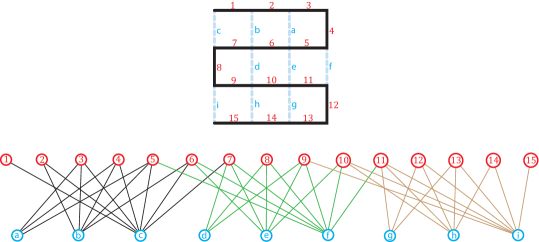
Figure 4. The bipartite graph of the centipede $T_{4}\subset G(4)$.

Example 10.1 (The Centipede Family).

We first study the centipede family $\mathcal{F}=\{T_{n}\subset G(n)\mid n\geq 3\}$. The bipartite graph of $T_{4}$ is shown in Figure 4. The degree-mass function $p_{n}$ of the centipede $T_{n}$ is particularly simple:

(10.1) $$p_{n}(d)=\frac{1}{n-1}\text{ for each }d\in\{3,5,...,2n-1\}.$$

Therefore for each $d\geq 3$, $p_{\infty}(d)=\lim_{n\rightarrow\infty}p_{n}(d)=0$, so $\mathcal{F}$ is convergent and its power series is

$$f(x)=1+x.$$

This power series encodes the fact that as $n\rightarrow\infty$, the approximate passing times for $T_{n}$ look more and more like the extreme case considered in the proof of the upper bound of Theorem 1.1; namely $\{\tilde{P}_{i}\}\approx\{N,N+1,...,N+M\}$.

The centipede family is bounded because Equation 10.1 says that the maximum degree in $\mathcal{V}_{2}$ equals $2n-1$, which become arbitrarily small relative to $n^{2}$. The centipede family is also neighbor-connected, as can be seen from the structure of the bipartite graph exemplified in Figure 4. A pair of nodes of $\mathcal{V}_{2}$ share a neighbor if and only if the corresponding chords are in the same or adjacent rows. Such pairs represent the full range of degrees in $\mathcal{V}_{2}$, so their degrees grow without bound.

Proposition 9.4 only provides the following old information.

$$Q(\mathcal{F})\geq\frac{1}{e\cdot\overline{f}}=\frac{1}{4}.$$

We do not know whether $Q(\mathcal{F})=\frac{1}{4}$.

Example 10.2 (The Double Spiral Family).

The double spiral family in Figure 1 is convergent and has the same power series as the centipede, namely $f(x)=1+x$. This family is not bounded because the average degree grows proportional to $M$. In fact, the family is designed to have high average degree growth, and hence be a good candidate for having the minimum possible decay base.

Example 10.3 (The Fractal Family).

We next study the fractal family $\mathcal{F}=\{F_{k}\subset G(2^{k})\mid k=1,2,...\}$. It is bounded because the average degree of nodes in the bipartite graph of $F_{k}\subset G(2^{k})$ grows logarithmically in $n=2^{k}$, as shown in [2].

Let $p_{k}$ denote the degree-mass function for $F_{k}$. Unlike the mass functions for the centipede family, these mass functions converge to non-zero limits.

Lemma 10.4.

For each $d\geq 3$, the sequence $\{p_{k}(d)\}$ converges to a limit, which we denote as $p_{\infty}(d)$, and $\sum_{k\geq 3}p_{\infty}(k)=1$.

Proof.

Let $q_{k}(d)$ denote the number of degree $d$ nodes in $\mathcal{V}_{2}$, so

(10.2) $$p_{k}(d)=\frac{q_{k}(d)}{|\mathcal{V}_{2}|}=\frac{q_{k}(d)}{2^{2k}-2^{k+1}+1}.$$

Fix a value $d\geq 3$. Assume it’s not the case that $q_{k}(d)=0$ for all $k$. We claim there exists an index $k_{0}$ beyond which $\{q_{k}(d)\}$ satisfies a simple first order linear recurrence relation with base $4$; that is:

$$q_{k+1}(d)=4\cdot q_{k}(d)+C\,\,\,\text{ for all }k\geq k_{0}.$$

The solution is:

$$q_{k_{0}+t}=\left(A+\frac{C}{3}\right)4^{t}-\frac{C}{3}\,\,\,\text{ for all }t\geq 0,$$

where $A=q_{k_{0}}(d)$. Therefore Equation 10.2 gives:

(10.3) $$\lim_{t\rightarrow\infty}p_{k}(d)=\frac{A+\frac{C}{3}}{4^{k_{0}}}.$$

To justify the recurrence relation, notice that each branch of $F_{k+1}$ either belongs to one of the four copies of $F_{k}$ out of which $F_{k+1}$ is built, or is a “cut branch” that connects two of these quadrants. Thus,

$$q_{k+1}(d)=4\cdot q_{k}(d)+C_{k+1}(d),$$

where $C_{k+1}(d)$ is the number of cut branches with degree $d$. We claim that for sufficiently large $k$, $C_{k+1}(d)$ doesn’t depend on $k$. To see this, consider the list of degrees of nodes in the set $\mathcal{V}_{2}$ from $F_{k+1}$ corresponding to cut branches. This list is naturally partitioned into two halves of equal length. The inner half is exactly the list from $F_{k}$, whereas the minimal degree for the outer half goes to infinity as $k\rightarrow\infty$.

From the above calculations, one can prove that the convergence is uniform: for every $\epsilon>0$ there exists $d_{0}$ such that $\sum_{d\geq d_{0}}p_{k}(d)<\epsilon$ for all $k\in\mathbb{N}$. From this it is straightforward to conclude that $\sum_{d\geq 1}p_{\infty}(d)=1$. ∎

Table 1 reports the value $p_{\infty}(d)$ for all $3\leq d\leq 125$, which we computed using Equation 10.3 and a computer.

The Fractal family $\mathcal{F}$ is neighbor-connected for the following reason. Define $\Delta_{k}=\mathcal{V}_{2}\times\mathcal{V}_{2}$ (in the bipartite graph associated to $T_{k}$), and let $\tilde{\Delta}_{k}$ be the set of pairs $(v,w)\in\Delta_{k}$ that have at least one common neighbor in $\mathcal{V}_{1}$. Due to the recursive definition of the family,

$$\frac{|\tilde{\Delta}_{k}|}{|\Delta_{k}|}\approx\frac{1}{4}\cdot\frac{|\tilde{\Delta}_{k-1}|}{|\Delta_{k-1}|}.$$

This is because chords from different quadrants have no common neighbors, and the contribution of the cut edges between the quadrants becomes negligible as $k\rightarrow\infty$. Therefore $\frac{|\tilde{\Delta}_{k}|}{|\Delta_{k}|}\rightarrow 0$.

Table 1. $p_{\infty}(d)$ for all $3\leq d\leq 125$ for the Fractal family

$d$	$3$	$5$	$11$	$13$	$25$	$27$	$29$	$55$	$57$
$p_{\infty}(d)$	$\frac{5}{12}$	$\frac{1}{4}$	$\frac{1}{12}$	$\frac{1}{12}$	$\frac{1}{96}$	$\frac{1}{24}$	$\frac{1}{32}$	$\frac{1}{384}$	$\frac{1}{128}$

$d$	$59$	$61$	$117$	$119$	$121$	$123$	$125$
$p_{\infty}(d)$	$\frac{7}{384}$	$\frac{5}{384}$	$\frac{1}{1536}$	$\frac{1}{384}$	$\frac{1}{256}$	$\frac{1}{128}$	$\frac{3}{512}$

Let $f$ be the power series for $\mathcal{F}$. Let $f^{+}$ denote polynomial approximations of $f$ obtained by truncating after the $x^{125}$ term. $\mathcal{F}$ is bounded and convergent, so we can apply Proposition 9.4, which yields the following.

$$Q(\mathcal{F})^{-1}\leq e\cdot\overline{f}\leq e\cdot\overline{f^{+}}=3.2508\cdots.$$

Adding more terms to $f^{+}$ improves this bound, but only slightly; in fact it can be shown that $e\cdot\overline{f}>\mathfrak{b}=3.2099\cdots$.

Example 10.5 (The Uniform Family).

Consider a family $\mathcal{F}=\{T_{n}\subset G(n)\mid n\in\mathbb{N}\}$ where each spanning tree $T_{n}$ is uniformly randomly chosen. We’ll call $\mathcal{F}$ a uniform family. Let $p_{n}$ denote the degree-mass function of $T_{n}$. Although the randomness means that $T_{n}$ and $p_{n}$ are not uniquely determined, the limit $p_{\infty}=\lim(p_{n})$ is uniquely determined with probability $1$ because it can be interpreted as the degree-mass function for a uniformly random spanning tree of the infinite lattice $\mathbb{Z}^{2}$. Manna et al. studied this situation in [20] and proved that $p_{\infty}(3)\approx 0.29454$ and $p_{\infty}(5)\approx 0.12409$ (these are decimal approximations of the exact values that they calculated). The also provided strong numerical and theoretical evidence for their conjecture that $d\mapsto p_{\infty}(d)$ decays as $d^{-8/5}$ for large $d$.

This conjecture indicates that the following is a reasonable approximation of the power series $f$ of $\mathcal{F}$:

$$f(x)\approx 2-x-(0.29454)x^{3}-(0.12409)x^{5}-C\cdot\sum_{d\geq 7\text{ odd }}d^{-8/5},$$

where $C$ is chosen to make it a valid probability mass function. This yields:

(10.4) $$e\cdot\overline{f}=3.433\cdots.$$

This is higher than the corresponding value for the fractal family, which is evidence that the fractal family has higher MST probability than does a uniform family, although we do not know whether the uniform family is bounded or neighbor-connected.

It is significant that the uniform family behaves qualitatively like fractals, not like centipedes (in the sense that $p_{\infty}$ is a valid probability function).

11. Questions and Conjectures

A natural open question is to identifying the optimal upper and lower bounds in Theorem 1.1, which will require the construction a family of spanning trees that achieves each bound. A potential starting point for addressing the lower bound is to answer the following.

Question 11.1.

Is the decay base of the double spiral family equal to $\frac{1}{4}$?

The fractal family $\mathcal{F}$ might not achieve the optimal upper bound, but it is reasonable to expect it to come close. This family was originally believed to be optimal for the related problem of minimizing average stretch, but families were later constructed that were slightly better [14],[19]. Proposition 9.4 only provided a lower bound for the decay base of the fractal family, but this bound isn’t sharp, so the following question remains.

Question 11.2.

What is the decay base of the fractal family?

One way to address this is to quantify how close the inequality in Proposition 9.4 comes to being an equality. Here is an concise overview of the proof of Proposition 9.4.

$$\text{Prob}_{\text{MST}}(T_{n}) \sim e^{-M}\cdot\mathbb{E}\left(\mathcal{A}(T_{n})^{-M}\right)\geq e^{-M}\cdot\left(\mathbb{E}(\mathcal{A}(T_{n}))\right)^{-M}$$

$$\sim e^{-M}\cdot\overline{f}^{-M}\sim\left(e\overline{f}\right)^{-n^{2}}$$

The only inequality here comes from Jensen’s Inequality, so it would be necessary to understand the Jensen Gap, which requires understanding how quickly the variance of $\mathcal{A}(T)$ decays with $M$. The following conjecture quantifies this.

Conjecture 11.3.

If $\mathcal{F}=\{T_{n}\subset G(n_{n})\mid n\in\mathbb{N}\}$ is a bounded, convergent, neighbor-connected family, and $f$ is its associated power series, then

$$Q(\mathcal{F})=\frac{\exp\left(\lim_{m\rightarrow\infty}\frac{(n\cdot\sigma_{n})^{2}}{2}\right)}{e\cdot\overline{f}},$$

where $\sigma_{n}^{2}$ denotes variance of the random variable $X_{n}=\ln(\mathcal{A}(T_{n}))$.

Sketch of potential proof idea.

Consider a fixed large value of $n$, an interpret all running notation with respect to the spanning tree $T=T_{n}$. The proof of Proposition 9.3 establishes that

$$\mathbb{E}(X)\approx\ln\overline{f}.$$

Let $\Psi$ be the moment generating function of $X$. Stirling’s approximation gives:

$$\Psi(-M) =\mathbb{E}\left(e^{-MX}\right)=\mathbb{E}\left(\prod\frac{M}{P_{i}(\alpha)}\right)=M^{M}\cdot\mathbb{E}\left(\prod\frac{1}{P_{i}(\alpha)}\right)$$

$$\approx e^{M}\cdot M!\cdot\mathbb{E}\left(\prod\frac{1}{P_{i}(\alpha)}\right)=e^{M}\cdot\text{Prob}_{\text{MST}}(T).$$

On the other hand, if we assume that $X$ becomes normal as $n\rightarrow\infty$, then $\Psi(t)\approx\exp\left(\mathbb{E}(X)t+\frac{\sigma^{2}}{2}t^{2}\right),$ so

$$\Psi(-M) \approx\frac{e^{(\sigma\cdot M)^{2}/2}}{\overline{f}^{M}}$$

Combining the previous two equations yields

$$\text{Prob}_{\text{MST}}(T)\approx\frac{e^{(\sigma\cdot M)^{2}/2}}{e^{M}\cdot\overline{f}^{M}}=\left(\frac{e^{\sigma^{2}M/2}}{e\cdot\overline{f}}\right)^{M},$$

from which the result follows. ∎

References

- [1] I. Abraham, Y. Bartal, and O. Neiman. Nearly tight low stretch spanning trees. In Proc. 49th IEEE Symp. on Foundations of Computer Science (FOCS), 2008.
- [2] Alon, N., Karp, R., Peleg, D., West, D., A Graph-Theoretic Game and its Application to the -Server Problem, Sian J. Comput., Vol 24, No. 1 pp. 78-100, February 1995.
- [3] Amaldi, E., Liberti, L., Maculan, N., Maffioli, F., Efficient edge-swapping heuristics for finding minimum fundamental cycle bases, C. C. Ribeiro and S. L. Martins, editors, WEA, volume 3059 of Lecture Notes in Computer Science, pages 14–29, Springer, 2004.
- [4] Amaldi, E., Liberti, L., Maculan, N., Mathematical models and constructive heuristics for finding minimum fundamental cycle bases, Yugoslav journal of Operations Reserach, 15 (1): 15–24, 2005.
- [5] Bartal, Y., Probabilistic approximation of metric spaces and its algorithmic applications, Proceedings of the 37th IEEE FOCS (1996) pp. 184–193.
- [6] Bartal, Y., On approximating arbitrary metrices by tree metrics, Proceedings of the 30th ACM STOC (1998), pp. 161–168.
- [7] Deo, N., Krishnomoorth, M., Prabhu, G., Algorithms for generating fundamental cycles in a graph, ACM Translactions on Mathematical Software, 8(1) (1982), pp. 26-42.
- [8] Cannon, S., Duchin, M., Rule, P., Randall, D., A reversible recombination chain for graph partitions, preprint
- [9] Y. Emek and D. Peleg, A tight upper bound on the probabilistic embedding of series-parallel graphs, SIAM J. Discrete Math., 23(4):1827–1841, 2009.
- [10] Emek, Y.,k-Outerplanar Graphs, Planar Duality, and Low Stretch Spanning Trees
- [11] Elkin, M., Emek, Y., Spielman, D., Tenh, S., Lower-Stretch Spanning Trees, 2005.
- [12] Faccharoenphol, J., Rao, S., Talwar, K., A tight bound on approximating arbitrary metrics by tree metrics, Proceedings of the 35th ACM STOC (2003), pp. 448-455.
- [13] Köhler, E., Liebchen, C., Wünsch, G., Rizzi, R., Lower Bounds for Strictly Fundamental Cycle Bases in Grid Graphs.
- [14] Köhler, E., Rizzi, R., Wünsch, G., Reducing the optimality gap of strictly fundamental cycle bases in planar grids, Preprint 007/2006, TU Berlin, Mathematical Institute, 2006.
- [15] Lavrov, Misha, Variance of a sample from a bipartite graph, Stack Exchange solution, https://math.stackexchange.com/q/4848665.
- [16] Liebchen, C., Finding short integral cycle bases for cyclic timetabling, Giuseppe Di Battista and Uri Zwick, editors, ESA, volume 2832 of Lecture Notes in Computer Science, pages 715–726. Springer, 2003.
- [17] Liebchen, C., Rizzi, R., A new bound on the length of minimum cycle bases
- [18] C. Liebchen and G. Wünsch. The zoo of tree spanner problems. Discrete Appl. Math., 156:569–587, 2008.
- [19] Liebchen, C., Wünch, G., Köhler, E., Reich, Al, Rizzi, R., Benchmarks for strickly fundamental cycle bases (2007)
- [20] Manna, M., Dhar, D., Majumdar, S., Spanning-Trees in 2 Dimensions, Physical Review A, Atomic, Molecular and Optional Physics, October 1992.
- [21] Narayanaswamy, N., Ramakrishna, G, On Minimum Average Stretch Spanning Trees in Polygonal 2-trees, 2014.
- [22] Rizzi, R., Liebchen, C., A new bound on the length of mimimum cycle bases (2006)
- [23] Lyons, R., Peres, Y., Minimal spanning forests, Ann. Probab., 34(5), pp. 1665–1692.
- [24] Wu, F., Number of spanning trees on a lattice. J. Phys. A, 10(6):L113–L115, 1977.
- [25] G. Wünsch, Coordination of Traffic Signals in Networks, Culviller Verlag, Göttingen, 2008.