Euclid preparation.

Verifying the fully kinematic nature of the long-known cosmic microwave background (CMB) dipole is of fundamental importance in cosmology. In the standard cosmological model with the Friedman–Lemaitre–Robertson–Walker (FLRW) metric from the inflationary expansion the CMB dipole should be entirely kinematic. Any non-kinematic CMB dipole component would thus reflect the preinflationary structure of spacetime probing the extent of the FLRW applicability. Cosmic backgrounds from galaxies after the matter-radiation decoupling, should have kinematic dipole component identical in velocity with the CMB kinematic dipole. Comparing the two can lead to isolating the CMB non-kinematic dipole. It was recently proposed that such measurement can be done using the near-IR cosmic infrared background (CIB) measured with the currently operating Euclid telescope, and later with Roman. The proposed method reconstructs the resolved CIB, the Integrated Galaxy Light (IGL), from Euclid’s Wide Survey and probes its dipole, with a kinematic component amplified over that of the CMB by the Compton–Getting effect. The amplification coupled with the extensive galaxy samples forming the IGL would determine the CIB dipole with an overwhelming signal-to-noise ratio, isolating its direction to sub-degree accuracy. We develop details of the method for the Euclid’s Wide Survey in four bands spanning 0.6 to 2 $\mathrm{\SIUnitSymbolMicro m}$. We isolate the systematic and other uncertainties and present methodologies to minimize them, after confining the sample to the magnitude range with negligible IGL/CIB dipole from galaxy clustering. These include the required star–galaxy separation, accounting for the extinction correction dipole using the method newly developed here achieving total separation, accounting for the Earth’s orbital motion and other systematic effects. Finally, we apply the developed methodology to the simulated Euclid galaxy catalogs testing successfully the upcoming applications. With the presented techniques one would indeed measure the IGL/CIB dipole from Euclid’s Wide Survey with high precision probing the non-kinematic CMB dipole.

1 Motivation

The cosmic microwave background (CMB) dipole is the oldest known CMB anisotropy of $\delta T_{\rm CMB}=3.35$ mK, or $\delta T_{\rm CMB}/T_{\rm CMB}=1.23\times 10^{-3}$, measured with the unprecedented precision of a signal-to-noise ratio of ${\rm S/N}\gtrsim 200$ (Kogut et al. 1993; Fixsen et al. 1994). It is conventionally interpreted as being entirely of kinematic origin due to the Solar System moving at velocity $V_{\rm CMB}=370$ km s^-1 in the Galactic direction of $(l,b)_{\rm CMB}=(263\aas@@fstack{\circ}85\pm 0\aas@@fstack{\circ}1,48\aas@@fstack{\circ}25\pm 0\aas@@fstack{\circ}04)$.

The fully kinematic origin of the CMB dipole is further motivated theoretically by the fact that any curvature perturbations on superhorizon scales leave zero dipole because the density gradient associated with them is exactly cancelled by that from their gravitational potential (Turner 1991). However, already prior to the development of inflationary cosmology there were suggestions that the CMB dipole may be, even if in part, primordial (King & Ellis 1973; Matzner 1980). Within the inflationary cosmology, which posits the non-Friedmann–Lemaitre–Robertson–Walker (FLRW) metric on sufficiently large scales due to the primeval (preinflationary) structure of space-time (Turner 1991; Grishchuk 1992; Kashlinsky et al. 1994; Das et al. 2021), such possibility can arise from isocurvature perturbations induced by the latter (Turner 1991) and/or from entanglement of our Universe with other superhorizon domains of the Multiverse (Mersini-Houghton & Holman 2009). Hence, establishing the nature of the CMB dipole is a problem of fundamental importance in cosmology.

Despite the overwhelming preference of the kinematic CMB dipole interpretation, there have been longstanding observational claims to the contrary (Gunn 1988). Comparing the gravity dipole with peculiar velocity measurements (Villumsen & Strauss 1987) indicates an offset (Gunn 1988; Erdoǧdu et al. 2006; Kocevski & Ebeling 2006; Lavaux et al. 2010; Wiltshire et al. 2013) broadly buttressed by other peculiar velocity data (Mathewson et al. 1992; Lauer & Postman 1992; Ma et al. 2011; Colin et al. 2019). There appears a “dark flow” of galaxy clusters in the analysis of the cumulative kinematic Sunyaev–Zeldovich effect extending to at least $\sim$1 Gpc in both WMAP and Planck data (Kashlinsky et al. 2008, 2009; Atrio-Barandela et al. 2010; Kashlinsky et al. 2010, 2012a; Atrio-Barandela 2013; Atrio-Barandela et al. 2015), which is generally consistent with the radio (Nodland & Ralston 1997; Jain & Ralston 1999; Singal 2011) and WISE (Secrest et al. 2021) source count dipoles and the anisotropy in X-ray scaling relations (Migkas et al. 2020). See reviews by Kashlinsky et al. (2012b); Aluri et al. (2023). All of these assertions have achieved only a limited significance of ${\rm S/N}\sim 3$–$5$, with the subsequently significant directional uncertainty, and are debated.

It is important to establish observationally the fully kinematic nature of the CMB dipole and whether the homogeneity in the Universe as reflected in the FLRW metric models is adequate to describe what we observe. Since any curvature perturbations must have zero dipole at last scattering such probe would be fundamental to cosmology with the non-kinematic CMB dipole component potentially providing a probe of the primordial preinflationary structure of spacetime. To this end a technique has been proposed recently by Kashlinsky & Atrio-Barandela (2022) to be applied to the Euclid Wide Survey to probe the dipole of the resolved part of the CIB, the IGL, at an overwhelming ${\rm S/N}$ thereby settling the issue of the origin of the CMB dipole.

Here we develop the detailed methodology for this experiment we call NIRBADE (Near IR BAckground Dipole Experiment) dedicated to measuring, at high ${\rm S/N}$, the (amplified) CIB dipole from the Euclid Wide Survey. In Sect. 2 we discuss the different physics governing CMB and CIB dipoles, pointing out how at the Euclid-covered wavelengths the expected kinematic CIB dipole will be significantly amplified over that of the CMB. Section 3 sums up the details of the Euclid Wide Survey and their application to NIRBADE following Kashlinsky & Atrio-Barandela (2022). Section 4 is devoted to the required development to achieve the NIRBADE goal covering the overall pipeline. These topics include isolating the needed magnitude range here (AB magnituudes are used throughout this paper), developing the methodology to successfully isolate the dipole from Galactic extinction, and accounting for the Earth’s orbital motion. Here, we also discuss a slew of less critical, but still important items, such as photometry, before moving on to quantifying the overall uncertainties expected in the pipeline. Section 5 then applies the development here to the simulated Euclid catalog to demonstrate how comparing the measured CIB dipole with the well known CMB dipole will isolate any non-kinematic CMB dipole component down to interestingly low levels. We sum up the prospects for NIRBADE with Euclid in Sect. 6.

More specifically the outline of the developmental part of the study is as follows:

• The procedure of the measurement with the required steps to be implemented here has been designed in Sect. 4.1. The procedure requires successfully finessing the various items that are subsequently outlined, discussed, and resolved.

• In the following Sect. 4.2 we present the pre-launch plan of the Euclid Wide Survey coverage that we use in the computations here. Now that the mission is at L2, the details of the survey may be altered, so this is given as an example used for development in finalizing the details of the methodology. The methodology developed here will be applied to the actual observed coverage.

• We identify the aspects required for selecting galaxies from the Euclid Wide Survey for this measurement in Sect. 4.3 – Eq. (9) for VIS and Eq. (10) for NISP. Throughout we used, in the absence of the forthcoming Euclid data, the observed galaxy counts presented in Sect. 4.3.1 for JWST measurements (Windhorst et al. 2023) and, when needed, the HRK reconstruction (Helgason et al. 2012). The range of galaxy magnitudes required to sufficiently reduce the clustering dipole component is isolated in Sect. 4.3.5. The prospects of the star–galaxy separation desired in the experiment are given in Sect. 4.3.2.

• Section 4.4 discusses how the extinction, using the SFD template (Schlegel et al. 1998), can affect the measurement and design a method to isolate the contribution due to extinction corrections from that of the IGL/CIB. The method is applicable at small extinction corrections $A\ll 1$.

• The needed corrections, for the high-precision measurement, from the effects of the Earth’s orbital motion are then discussed in Sect. 4.5. It is shown how the corrections will be incorporated into the designed pipeline.

• The potential systematic effects, and how to correct for them are considered in Sect. 4.7 followed by the requirements on the photometric accuracy and zero points, etc. in Sect. 4.8.

• Section 5 then shows the application of the developed methodology to the forthcoming Euclid Wide Survey data. In Sect. 5.1 we evaluate the statistical uncertainties after each year of the Euclid observation. In Sect. 5.2 we apply the method developed here to correct for extinction using a simulated catalog for Euclid with available spectral colors, to isolate the contribution from extinction if the need arises in the actual data to finalize the high-precision determination of the IGL/CIB dipole from the Euclid Wide Survey. Section 5.3 discusses and quantifies the identified systematic corrections when converting the measured IGL/CIB dipole into the equivalent velocity, which affect all the velocity components equally thereby being of relevance to its amplitude, and not direction.

Such an experiment can, and must, also be done with Roman (formerly WFIRST; Akeson et al. 2019), which would require a separate and significantly different preparation.

2 On importance of cosmic background dipoles

Here we discuss the different physics governing the CMB and CIB dipoles and why and how the CIB kinematic dipole is amplified over that of the CMB.

2.1 On the intrinsic CMB dipole

The CMB as observed today originates at the last scattering, which occurred at the cosmic epochs corresponding to redshift $z\simeq 10^{3}$. Its structure from the quadrupole term ($\ell=2$) to higher-order in $\ell$ multipoles is in very good general agreement with predictions of inflation. The latter posits that the observed Universe originated from a small smooth patch, with the underlying FLRW metric, of the size of or smaller than the horizon scale at the start of inflation, which then quickly inflated to encompass scales well beyond the current cosmological horizon (Kazanas 1980; Guth 1981). At the same time, on sufficiently large scales the preinflationary spacetime could have preserved its original structure, assumed generally to be inhomogeneous (Turner 1991; Grishchuk 1992; Kashlinsky et al. 1994). Such preinflationary structures, currently on superhorizon scales, could leave CMB signatures via the Grishchuk–Zeldovich effect (Grishchuk & Zeldovich 1978). The smallness of the measured CMB quadrupole (the relative value of $Q\sim 2\times 10^{-6}$) indicates that preinflationary structures in spacetime were pushed during inflation to scales currently $\gtrsim Q^{-1/2}cH_{0}^{-1}\sim 10^{3}cH_{0}^{-1}$ (Turner 1991; Kashlinsky et al. 1994).

However, as was shown by Turner (1991), the Grishchuk–Zeldovich effect does not produce an observable dipole anisotropy in any superhorizon modes from curvature perturbations because at the last scattering the linear gradient associated with them is cancelled exactly by the corresponding dipole anisotropy from their gravitational potential term. This points to the unique importance of probing the fully kinematic nature of the CMB dipole where any non-kinematic dipole would arise from, within the inflationary paradigm, the preinflationary structure of spacetime and potentially provide new information on the details of inflation and the applicability limits of the FLRW metric.

This differentiates the CMB dipole from the dipole components of the cosmic backgrounds, discussed next, which are produced by sources that formed well after decoupling.

2.2 The Compton–Getting effect and dipole for cosmic backgrounds from galaxies

Cosmic backgrounds produced by luminous sources that formed at $z\ll 10^{3}$ are subject to a different physics and their spatial distribution is imprinted during the inflationary period and later modified by the standard gravitational evolution during radiation-dominated era. In addition if the Solar System moves with respect to the frame defined by distant sources producing the background with mean intensity $\bar{I}_{\nu}$ at frequency $\nu$, it would have a dipole in the Sun’s rest frame

$$\boldsymbol{d}_{\nu}=(3-\alpha_{\nu,\infty})\frac{\boldsymbol{V}}{c}\bar{I}_{\nu,\infty}\,,$$ (1)

where

$$\alpha_{\nu}=\frac{\partial{\ln I_{\nu}}}{\partial{\ln\nu}}$$ (2)

and the subscript $\infty$ implies that the background intensity $I_{\nu}$ comes from integrating over the entire range of fluxes/magnitudes of the contributing sources. This is known as the Compton–Getting (Compton & Getting 1935) effect for cosmic rays (e.g. Gleeson & Axford 1968). Equation (1) follows since photons emitted at frequency $\nu_{0}$ from a source moving at velocity $V\ll c$ forming angle $\Theta$ toward the apex of motion will be received by the observer at rest at frequency $\nu=\nu_{0}[1+({V}/{c})\cos\Theta]$ and the Lorentz transformation requires that $I_{\nu}/\nu^{3}$ remains invariant (Peebles & Wilkinson 1968). Hence the observer at rest will see the direction-dependent specific intensity $I_{\nu}=(\nu/\nu_{0})^{3}I_{\nu/[1+({V}/{c})\cos\Theta]}$; see Appendix. The spectral index of the Rayleigh-Jeans spectrum $\alpha_{\nu}^{\rm RJ}=2$ describes the CMB at mm wavelengths.

If the CMB is the rest frame of the Universe then $\boldsymbol{V}=\boldsymbol{V}_{\rm CMB}$ for any cosmic background that originates from galaxies. Otherwise, the non-zero non-kinematic part of the CMB dipole would be likely to indicate the existence of superhorizon deviations from the FLRW metric, possibly due to the primordial (preinflationary) structure of spacetime.

At wavelengths where cosmic backgrounds from galaxies have $\alpha_{\nu}\ll 2$, the amplitude of their kinematic dipole in $I_{\nu}$ is amplified. This is the case for CIB (Kashlinsky 2005) and is also the case at high energies [X-ray (Fabian & Warwick 1979) and $\gamma$-ray (Maoz 1994; Kashlinsky et al. 2024) backgrounds, and cosmic rays (Kachelrieß & Serpico 2006)]. However, at infrared wavelengths significant pollution to the CIB dipole would come from dust emission and reflection by the Galaxy (cirrus) and the Solar System (zodiacal light) as discussed in Kashlinsky & Atrio-Barandela (2022).

3 Probing the near-IR background dipole in the Euclid Wide Survey

The Euclid satellite was successfully launched on July 1, 2023 to the L2 orbit. The photometric bands covered by Euclid are shown in Fig. 1. The unresolved CIB dipole at the Euclid bands will be subject to significant contributions from Galactic and Solar System foregrounds, but the foreground dipole contributions can be excluded efficiently by considering the CIB from resolved galaxies.

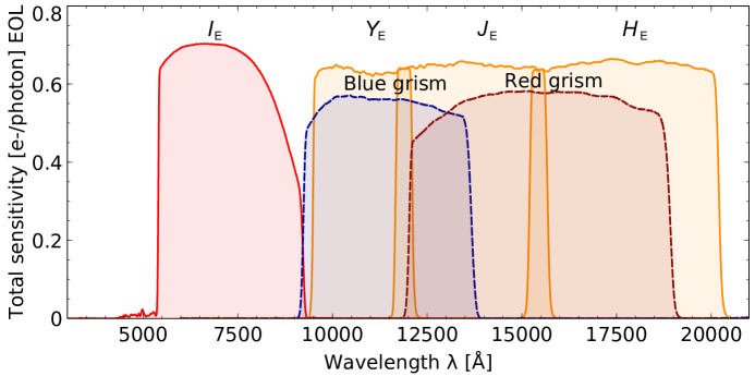
Figure 1: Total sensitivity of Euclid’s photometric and spectroscopic bands. (credit:ECSURV/J.-C. Cuillandre)

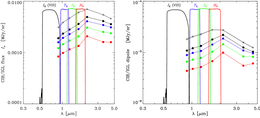
Figure 2: Left: The mean IGL flux. Right: The IGL dipole per Eqs. (2) and (3) and assuming $V=370$ km s^-1. Black plus signs correspond to the entire range of magnitudes. Black, blue, green, and red circles correspond to IGL from galaxies at $m\geq 18,19,20,21$. The IGL is integrated over the JWST latest counts (Windhorst et al. 2023) at the marked central wavelengths.

To overcome the obstacles due to the otherwise dominant at near-IR foreground dipoles Kashlinsky & Atrio-Barandela (2022) proposed to use the all-sky part of the background, known as IGL (Integrated Galaxy Light), reconstructed from resolved galaxies in the Euclid Wide Survey (Laureijs et al. 2011),

$$I_{\nu}(\theta,\phi)=10^{-0.4A_{\nu}(\theta,\phi)}S_{0}\int_{m_{0}}^{m_{1}}10^{-0.4m}\left[\frac{{\rm d}N_{\nu}(\theta,\phi)}{{\rm d}m}\right]{\rm d}m\,,$$ (3)

where $S_{0}=3631$ Jy and $A_{\nu}$ is the magnitude extinction in the direction $(\theta,\phi)$. The above expression is a short-hand for the actual procedure outlined in Sec. 4.1, Eq. (7) which requires no source counts determination. The Euclid Wide Survey galaxy samples will be corrected for extinction, so strictly speaking $A_{\nu}$ should be interpreted as the magnitude correction remaining after the extinction correction; more on this will be presented later. The IGL is evaluated over a suitably selected $m_{0}\sim 18$–$21$ required to remove the galaxy clustering dipole and $m_{1}$ imposed by the sensitivity limits of the Wide Survey, which is also below the expected magnitudes of the new populations expected to be present in the CIB source-subtracted anisotropies (Kashlinsky et al. 2018).

As discussed in Kashlinsky & Atrio-Barandela (2022) at the Euclid VIS and NISP bands $\alpha_{\nu}\sim-1$, so from an all-sky catalog of $N_{\rm gal}$ galaxies and for a fixed direction, one would reach the statistical signal-to-noise ratio in the measured IGL dipole amplitude, $d_{\nu}/\langle I_{\nu}\rangle$, of

$${\rm S/N}\sim 160\left(\frac{3-\alpha_{\nu}}{4}\right)\left(\frac{V}{V_{\rm CMB}}\right)\left(\frac{N_{\rm gal}}{10^{9}}\right)^{1/2}\,.$$ (4)

An all-sky CMB dipole measured with a signal-to-noise ratio of ${\rm S/N}$ will have its direction probed with directional accuracy of (Fixsen & Kashlinsky 2011)

$$\Delta\Theta_{\rm dipole}\sim\sqrt{2}({\rm S/N})^{-1}\;{\rm radian}\,.$$ (5)

This demonstrates that the directional uncertainty, say $\Delta\Theta_{\rm dipole}\lesssim 1^{\circ}$, needed to decisively probe the alignment requires ${\rm S/N}\gtrsim 80$. The statistical significance will depend on the actual dipole amplitude, direction and region of the sky observed by Euclid. For a partial sky coverage the above order of magnitude estimates will be reduced since the three dipole components $(X,Y,Z)$ will have different errors (Atrio-Barandela et al. 2010; Kashlinsky & Atrio-Barandela 2022). A discussion of the error budget is deferred to Sect. 5.1.

Equations (4) and (5) demonstrate why the to-date probes of the kinematic nature of the CMB dipole discussed in sec. 1, which reach ${\rm S/N}\simeq 4$–$5$ by utilizing the cumulative kinematic Sunyaev-Zeldovich (Sunyaev & Zeldovich 1980) effect (Kashlinsky & Atrio-Barandela 2000) or the relativistic aberration (Ellis & Baldwin 1984), have poor directional accuracy of $\Delta\Theta_{\rm dipole}\sim 15^{\circ}$–$20^{\circ}$ and hence are insufficient to test, in addition to the dipole amplitude and its convergence with distance, the consistency of the dipole directions. Both will be achieved with NIRBADE as outlined below.

Figure 2 (left) shows the IGL reconstructed from integrating over magnitudes exceeding some fiducial $m_{0}$ (see caption) using observed galaxy counts from Figs. 9 and 10 of the JWST counts data by Windhorst et al. (2023) at the wavelengths similar to the Euclid bands. The right panel of the figure shows the expected dipole amplitudes evaluated with Eq. (2) for $V=V_{\rm CMB}=370$ km s^-1. Plus signs mark the entire range out to the Euclid Wide Survey limit of $m_{1}=24$. Circles mark the results for $m_{0}\leq m\leq m_{1}$ for $m_{0}=18$, 19, 20, and 21 (black, blue, green, and red) and $m_{1}=25$. The four Euclid filters are shown per Euclid Collaboration: Schirmer et al. (2022). Later we will discuss the selections of $(m_{0},m_{1})$ required specifically for this measurement.

4 Required development

If the CMB dipole is entirely kinematic, the expected CIB dipole components in the Galactic coordinate system $(X,Y,Z)$ would be

$$\boldsymbol{d}_{\nu}=5.2\times 10^{-3}\left(\frac{3-\alpha_{\nu}}{4}\right)(-0.07,-0.66,0.75)\langle I_{\nu}\rangle\,,$$ (6)

with the $X$-component being by far the smallest, contributing just a few percent to the net dipole, and the $Z$-component being the largest, but close in amplitude to the $Y$-component. Hence, if the CMB dipole is purely kinematic, the IGL/CIB dipole, after correcting for the Earth motion, should lie almost entirely in the $(Y,Z)$ plane with nearly equal amplitude $Y$ and $Z$ components.

We are aiming to measure the IGL dipole of dimensionless amplitude of $\simeq 0.5\%$ in each or any of the Euclid’s four bands: $I_{\scriptscriptstyle\rm E}$, $Y_{\scriptscriptstyle\rm E}$, $J_{\scriptscriptstyle\rm E}$, and $H_{\scriptscriptstyle\rm E}$. Two points make this promising: 1) the IGL dipole is amplified by the Compton–Getting effect, and 2) the noise is substantially decreased by the large number of galaxies the Euclid Wide Survey will have.

Below are the items to discuss in order to get this measurement done, and at high precision. In what follows the sought dipole signal, Eq. (1), is denoted with a lower case $\boldsymbol{d}$ and the nuisance dipoles with a capital case $\boldsymbol{D}$.

In the absence of the Euclid data we will use here, for the bulk of estimates, the formulation per Eq. (3) inputting the latest JWST counts data from Windhorst et al. (2023), which are consistent with the reconstruction from Helgason et al. (2012) used originally by Kashlinsky & Atrio-Barandela (2022).

Depending on the context throughout this section we will work with both the absolute CIB dipole amplitude ($d_{\nu}$ in MJy sr^-1 equivalent to $\delta T$ in mK for the CMB) and its relative amplitude ($d_{\nu}/I_{\nu}$ equivalent to $\delta T/T$ for the CMB). The former would be useful when e.g discussing the measurability and overcoming the Galactic components while the latter is useful when estimating the extragalactic non-kinematic terms and converting to velocity.

4.1 Procedure

The procedure required to apply the method of Kashlinsky & Atrio-Barandela (2022) to probe the kinematic component of the IGL/CIB dipole would go through the following steps:

1. We will subdivide the Euclid sky coverage into areas, ${\cal A}$, centered on Galactic coordinates $(l,b)$. ${\cal A}$ could be the size of each FOV (0.5 deg²) or larger.

2. We will collect the photometry on all galaxies in each ${\cal A}$, with care to exclude Galactic stellar sources from the sample.

3. We will apply extinction corrections in each band and/or test for contributions from the extinction effects on the dipole by band, latitude etc. Then a method developed below to eliminate the extinction induced dipole will be applied.

4. We will identify, in each of the four Euclid photometric bands, the uniform upper magnitude limit, $m_{1}$, that can be applied to all selected regions ${\cal A}$. This would be one of the important criteria for selecting the sky for this measurement.

5. We will select a lower magnitude limit, $m_{0}$, to ensure the IGL dipole from galaxy clustering is sufficiently negligible. We may choose the same $m_{0}$ for each bands or leave it band-dependent, provided the clustering dipole contribution is negligible in all four Euclid bands.

6. We will compute the net IGL flux from the selected galaxies as

   $$I_{\nu}(l,b)=\frac{1}{{\cal A}}S_{0}\sum_{m_{0}\leq m\leq m_{1}}10^{-0.4m_{\nu}}$$ (7)

   over ${\cal A}$ and do this for the entire sky, or a selected part of it. Here $S_{0}=$3631$$ Jy.

7. We will evaluate the IGL dipole, $d_{\nu}$, over the selected Euclid sky in each of the four bands of frequency $\nu$ after dividing the galaxy sample by color to eliminate extinction.

8. We will eliminate the dipole contribution from extinction from a subsample of galaxies with selected IGL spectral index, $\alpha_{\nu}$, and isolate the kinematic IGL dipole part.

9. We will compute the dipole error.

10. We will evaluate the other systematics discussed below.

11. We will translate into the effective velocity via the refined estimation, for each galaxy subsample, of the IGL spectral index $\alpha_{\nu}$ and the Compton–Getting amplification using

    $$V=(3-\alpha_{\nu})^{-1}\left(\frac{d_{\nu}}{\langle I_{\nu}\rangle}\right)c\,.$$ (8)

We use HEALPix remove_dipole routine (Górski et al. 2005) in the computations throughout the paper.

4.2 Euclid Wide Survey galaxy samples

The Euclid Wide Survey aims to cover most of the best parts of the extragalactic sky in terms of extinction and star density. An area larger than $14\,000$ deg² is expected to be covered with a single visit (four exposures via three dithers). In each visit imaging data are acquired over 0.53 deg² for a wide visible band, $I_{\scriptscriptstyle\rm E}$   (sampling $0\aas@@fstack{\prime\prime}1$), and three near infrared bands ($Y_{\scriptscriptstyle\rm E}$, $J_{\scriptscriptstyle\rm E}$, and $H_{\scriptscriptstyle\rm E}$), where the sampling is $0\aas@@fstack{\prime\prime}3$.

In Fig. 3 the latest planned sky coverage is shown. There are three main contiguous areas that are covered [the fourth, that was presented in Fig. 45 of Euclid Collaboration: Scaramella et al. (2022), is now greatly reduced because of the lack of timely ground based photometry]. Grey regions denote unobserved areas due to the presence of extremely bright stars.

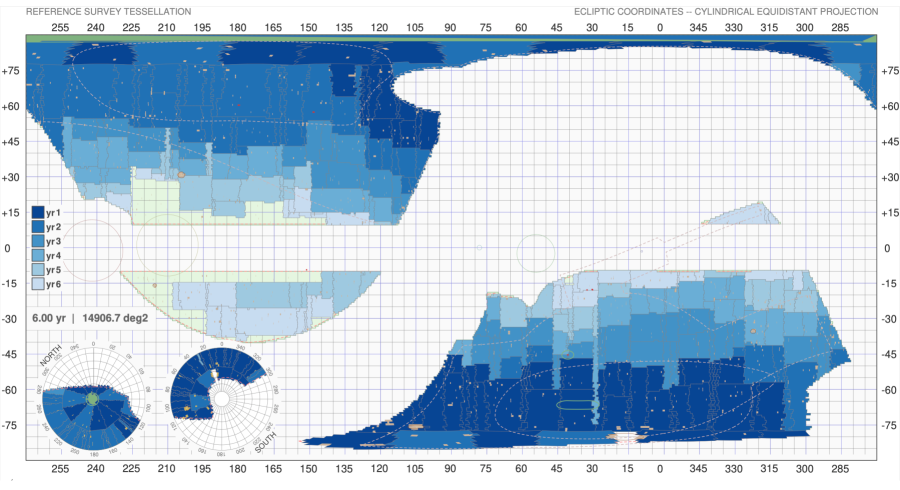
Figure 3: Expected coverage of the sky year by year of the wide survey in ecliptic coordinates. The ecliptic poles are also shown in a different projection. Circles along the ecliptic denote planet avoidance regions circa 2029 Sep 27, near the end of the survey. (credit: ECSURV/J.Dinis)

We focus in this subsection on the galaxy number density in $H$ band, which is the one least affected by extinction. Deep galaxy counts in $i$ and $K$ bands have been given by studies of the COSMOS field (Laigle et al. 2016; Weaver et al. 2022). Here we are mostly concerned with the intermediate range of magnitudes $20\leq m_{H}\leq 24$, which is appropriate to get a uniform sample from the Euclid Wide Survey.

These literature estimates, however, are affected by cosmic variance (Abbott & Wise 1984): the COSMOS area covers only 2 deg² and therefore is different from the average value taken on much larger areas. Moreover, we will need to work with several sub areas of the wide survey because of cuts to get subsamples and different epochs of increasing coverage.

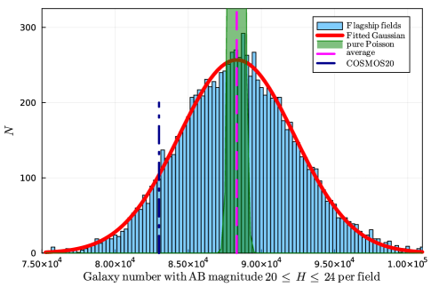
Figure 4: Distribution of simulated counts per Euclid field (half square degree).

Therefore we derive, for the time being, the impact of cosmic variance on the $H_{\scriptscriptstyle\rm E}$   counts from the Euclid Flagship simulation. From the large N-body simulation, the Flagship catalogue of many observables was derived. Of particular importance is the color-color relation and photo-$z$ distribution obtained by imposing spectral energy distributions to the halos identified as galaxies in the simulation. Therefore the parent spatial halo/galaxy distribution is clustered and so the catalogue 2D sample has an intrinsic angular correlation, which causes the distribution in cells to deviate from the simple Poisson distribution. How large the deviation is would be a function of both the limiting magnitude and the area considered.

In Fig. 4 we show how cosmic variance (Abbott & Wise 1984) affects the counts in a single Euclid field: the standard deviation, $\sigma$, is ${\sim}\,14$ times larger than the simple Poisson one due to clustering of the sources (Abbott & Wise 1984). We also show the counts from the COSMOS2020 catalog (Weaver et al. 2022). At this scale the $\sigma$ is still ${\sim}\,5\%$ of the average, but in simply increasing the basic area considered, this ratio will greatly decrease.

The total expected number density of galaxies is ${\sim}\,1.8\times 10^{5}$ deg^-2, which yields a total of $>2.5$ billion objects from the whole survey.

4.3 Selecting the optimal magnitude range $[m_{0},m_{1}]$

4.3.1 Galaxy counts

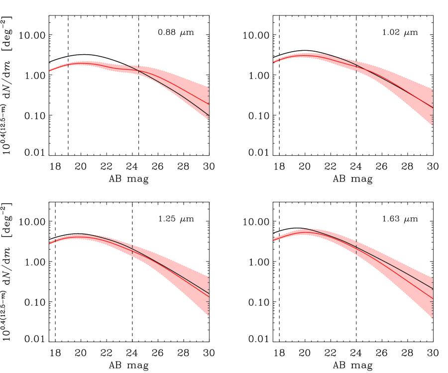
Figure 5: Galaxy counts per ${\rm d}m$, plotted $\propto{\rm d}I_{\nu}/{\rm d}m$, at the four sets of Euclid-related wavelengths. Black lines show the JWST counts at 0.88, 1.02, 1.25, and 1.63 $\mathrm{\SIUnitSymbolMicro m}$. HRK reconstructions are displayed with red colors, going to the 0.8 $\mathrm{\SIUnitSymbolMicro m}$ at the VIS-related end. The spreads in the reconstructions between the LFE (low-faint-end) and HFE (high-faint-end) limits of the extrapolation allowed for the Schechter-type luminosity function (Helgason et al. 2012) are shown with pink shades. Dashed vertical lines mark the range of magnitudes identified for this study in Eq. (10). The JWST counts are filter-transformed to either ground-based VISTA filters or Spitzer filters at the long wavelengths (S. Tompkins, R. Windhorst, private communication). HRK reconstructions are shown at the wavelengths of 0.8, 1.05, 1.25, and 1.63 $\mathrm{\SIUnitSymbolMicro m}$.

Throughout this discussion we will need the numbers for total galaxies expected to be available from the Euclid Wide Survey in the given magnitude range at the appropriate wavelengths. Such information is available from the recent JWST counts (Windhorst et al. 2023) and we will be using also the HRK reconstruction (Helgason et al. 2012) used in the pre-JWST era by Kashlinsky & Atrio-Barandela (2022); we will use both intermittently in our numerical estimates. Figure 5 shows the comparison at Euclid-related wavelengths of the HRK reconstruction (red) and the JWST counts for the Euclid bands. Figure 6 shows the same for the longer bands adjacent to NISP, which will be used later in Sect. 5. The VIS-related numbers are shown at 0.88 $\mathrm{\SIUnitSymbolMicro m}$ for JWST data and 0.8 $\mathrm{\SIUnitSymbolMicro m}$ for the HRK reconstruction mimicking the fits to the broad $I_{\scriptscriptstyle\rm E}$   band. The overall comparison shows good consistency, within the uncertainties, between the HRK reconstruction and JWST data, indicating that the former can be used for the power estimates below.

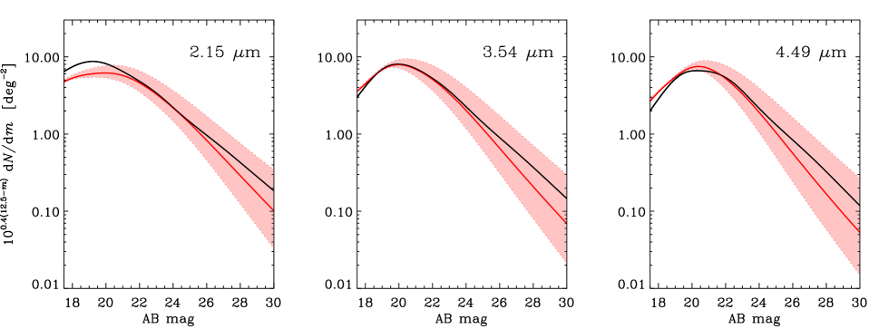
Figure 6: Same as Fig. 5, except at the wavelengths longward of, but adjacent to the NISP bands, which are used for refinements in $\alpha_{\nu}$ (e.g. Fig. 2 and Sect. 5). The JWST counts are filter-transformed to either ground-based VISTA filters or Spitzer filters at the long near-IR wavelengths (S. Tompkins, R. Windhorst, private communication). HRK reconstruction is shown at the wavelengths of 2.2, 3.6, and 4.5 $\mathrm{\SIUnitSymbolMicro m}$.

The quantities, $10^{0.4(12.5-m)}{\rm d}N/{\rm d}m$, plotted on the vertical axis in the figures directly reflect the IGL/CIB produced by galaxies in the ${\rm d}m$ range of $m$. The value of 1 deg^-2 on the vertical axis of Figs. 5 and 6 corresponds to ${\rm d}I_{\nu}/{\rm d}m=1.2\times 10^{-4}$ MJy sr^-1.

4.3.2 Star–galaxy separation

Galactic stars need to be excluded from the Euclid source counts when constructing the IGL. At wavelengths from 1 to 5 $\mu$m prior studies indicate that stars outnumber galaxies at $m\lesssim 18$ (e.g. Ashby et al. 2013; Windhorst et al. 2022, 2023). Thus, star–galaxy separation is essential if $m_{0}<18$ and still important for sources with $m>18$.

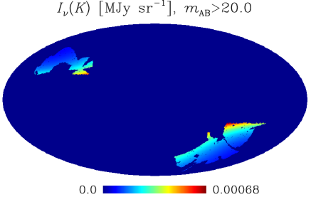
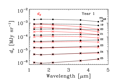
Figure 7: Top: The SKY model evaluated at $K$ band for stars with $m>20.0$. Intensities are in units of MJy sr^-1 and are masked at $|b|<20\degr$ (left) and for Year 1 of Euclid (right). Middle: The monopole amplitude of the SKY model as a function of wavelength and the bright magnitude limit. Bottom: The dipole amplitude of the SKY model as a function of wavelength and the bright magnitude limit. For the $|b|<20\degr$ mask (left) only the dominant $X$-component of the dipole is plotted. For the Year 1 mask (right) the total dipole is shown in black, and the $X$-component is shown in red. At these magnitude cuts and for these masks, the brightness and dipole of the model are dominated by the halo component, which is a spherical distribution of stars, peaked towards the Galactic center ($+X$).

To assess the possible dipole arising from Galactic stars, if they are incompletely excluded from catalogs used to construct the IGL, we evaluated the SKY model (Wainscoat et al. 1992; Cohen 1993, 1994, 1995) as implemented by Arendt et al. (1998), at a variety of wavelengths, and with cuts imposed to exclude stars brighter than chosen magnitude limits. Figure 7 shows the sky brightness predicted by the SKY model, with masking applied generically for $|b|<20\degr$ (left column) and specifically for Euclid Year 1 (right column). We ran the HEALPix routine remove_dipole on these masked models. The second row of Fig. 7 shows the derived monopoles. For the $|b|<20\degr$ mask, the third row shows the $X$-components of the dipoles ($Y$- and $Z$-components are orders of magnitude smaller). For the Year 1 mask, the third row shows the sum of all three dipole components (black), and the $X$-components only (red). For this masking, the $X$-component is only dominant at fainter magnitudes because the $X$ direction (towards the Galactic bulge) is not well sampled. The dipole amplitudes confirm that if stars are not excluded efficiently to faint magnitudes, then they may contaminate the IGL with a significant dipole. To probe the IGL dipole at the levels from Fig. 2, we need to eliminate either $>99\%$ of the stars or choose sufficiently faint $m_{0}$, while keeping enough galaxies to ensure good ${\rm S/N}$. Figure 10 shows that even if strict magnitude cuts are needed to exclude stars, there should be sufficient numbers of galaxies.

At the high latitudes of the Wide Survey, Gaia DR3 thoroughly samples the stellar disk populations and reaches into the Galactic halo. On the basis of Gaia DR3 proper motions, it will be possible to reliably exclude Galactic stars to Gaia’s $G\sim 21.4$ mag or $\sim$9 $\mu$Jy (Vallenari et al. 2022). Stars will only be a minority of all Euclid detections fainter than this limit. The Euclid pipeline will provide a flag in the final MER catalog indicating whether a detected source is a Galactic star, with a 1% error rate. Thus by combining Gaia and standard pipeline products it will be possible to reduce the level of stellar contamination by the required amount. In addition, star contamination can be entirely eliminated if one restricts the galaxy sample to the one that will be used for WL measures, that is objects with $I_{\scriptscriptstyle\rm E}$ size larger than $1.2\,{\rm PSF_{FWHM}}$ (Laureijs et al. 2011).

To estimate the extinction using different galaxy subsets as proposed here (Sect. 4.4.2), the subsets must be drawn from the same area of the sky such that the dipole due to extinction, $\boldsymbol{D}_{A}$, is unchanged, but there is no requirement that the subsets be complete in terms of source morphology. So while including some stars in the IGL calculation would generate systematic errors, there is no systematic error if the exclusion of Galactic stars is conservative and some galaxies are excluded because they are mistaken for stars.

4.3.3 Dipole contribution from clustering: $m_{0}$

The lower limit on the magnitude of galaxies selected for this measurement is dictated by the requirement that the contribution to the probed dipole from their clustering is sufficiently lower than the one from the Compton–Getting effect produced by our motion, which is expected to be ${\sim}\,(4.75$–$5.75)\times 10^{-3}(V/V_{\rm CMB})$ as displayed later in Fig. 23. We have evaluated the dimensionless amplitude, $\sqrt{C_{1}}/\langle I_{\nu}\rangle$, of the clustering dipole using the HRK reconstruction as described in Kashlinsky & Atrio-Barandela (2022), which is shown in Fig. 8. The figure shows that for that term to be comfortably below the Compton–Getting terms one would want to select galaxies at $m_{0}\gtrsim 19$ in the VIS sample and $m_{0}\gtrsim 18$ for the NISP galaxies.

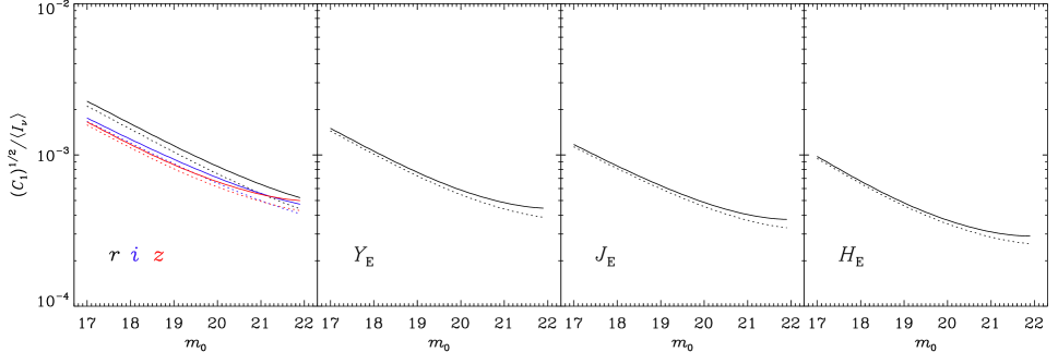
Figure 8: Dimensionless dipole from clustering evaluated from the HRK reconstruction as described in Kashlinsky & Atrio-Barandela (2022). The left panel includes the three photometric bands used by HRK that are covered by the wide $I_{\scriptscriptstyle\rm E}$ channel. Solid lines correspond to $m_{1}=24.5$ for $r$, $z$, and $i$, and $m_{1}=24$ for $Y_{\scriptscriptstyle\rm E}$, $J_{\scriptscriptstyle\rm E}$, and $H_{\scriptscriptstyle\rm E}$ bands, and dotted lines are for 0.5 magnitude fainter. This is to be compared to ${\sim}\,(4.75$–$5.75)\times 10^{-3}(V/V_{\rm CMB})$ as displayed later in Fig. 23.

In real situation, post-launch we will compute the power from the dipole-subtracted IGL maps, then extrapolate from higher (say, $\ell\gtrsim 10$–$20$) harmonics to $\ell=1$ using (after verifying) the Harrison–Zeldovich spectrum ($C_{\ell}\propto\ell$). For now we already have 1/8 of the sky from Flagship2.1 (via CosmoHub) simulations. Uniformity of $m_{0}$ across the sky also can be tested via the uniformity of the shot-noise power component in source-subtracted CIB achieved from the source-subtracted CIB studies with Euclid (Kashlinsky et al. 2018).

4.3.4 Choice of $m_{1}$

Figure 9: Contours show the decimal log of the expected number ($J_{\scriptscriptstyle\rm E}$ band) of galaxies [from Fig. 11 of Windhorst et al. (2023)] as a function of $m_{1}$ and area, for $m_{0}=18$. The dots mark the nominal $m_{1}=24$ and survey area expected after each addition year of the Wide Survey.

Euclid Collaboration: Scaramella et al. (2022) show that the Euclid Wide Survey is expected to reach its intended limiting magnitudes of $I_{\scriptscriptstyle\rm E}=24.5$ ($10\sigma$ extended source), and $Y_{\scriptscriptstyle\rm E},\ J_{\scriptscriptstyle\rm E},\ H_{\scriptscriptstyle\rm E}=24$ ($5\sigma$ point source) (Laureijs et al. 2011). So we will assume these values for $m_{1}$. In practice, a brighter limit for $m_{1}$ may be helpful for better source flux accuracy and potentially more reliable star galaxy separation. Conversely, it should be possible to choose a fainter limit for $m_{1}$ (up to ${\sim}\,1$ mag), though at the cost of limiting the analysis to a smaller fraction of the sky. These more sensitive regions (due to low zodiacal and Galactic foregrounds) will be covered in the earlier years of the survey. However in general, given the relatively shallow slope of galaxy counts at $m_{1}\sim 24$, it is better to choose larger rather than deeper areas in order to maximize the number of sources used for computing the IGL, and maximize the ${\rm S/N}$ of its dipole measurement. The expected galaxy counts as a function of survey area and $m_{1}$ are shown in Fig. 9.

4.3.5 The overall magnitude range required here

Thus we concentrate on galaxies in the magnitude range of

$$19\leq m\leq 24.5\hskip 56.9055pt{\rm VIS}\,,$$ (9)

$$18\leq m\leq 24\hskip 56.9055pt{\rm NISP}\,.$$ (10)

In the following sections we will select galaxies from the available simulation catalog according to Eqs. (9) and (10).

Figure 10 shows the number of galaxies expected around the required magnitude range using the JWST counts from Windhorst et al. (2023). Given that the statistical uncertainty is $\propto 1/\sqrt{N_{\rm gal}}$, we expect to have only minor variations in the uncertainty as the magnitude range is refined if necessary.

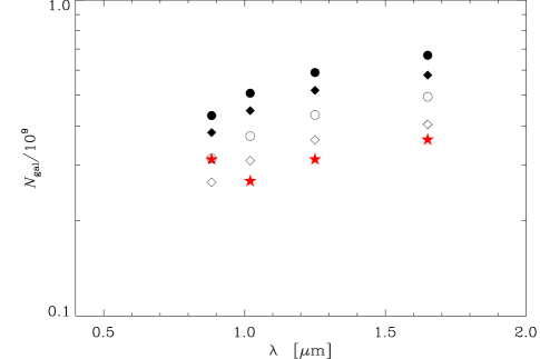
Figure 10: Number of galaxies after Year 1 of $2550$ deg² coverage for $m_{0}\leq m\leq m_{1}$. Circles correspond to $m_{0}=18$ and diamonds to $m_{0}=22$. Filled/open symbols correspond to $m_{1}=25/24.5$. Red asterisks show the numbers for the range in Eqs. (9) and (10) using the JWST counts (Windhorst et al. 2023).

4.4 Understanding details of extinction in the measurement

4.4.1 Extinction

Extinction from dust in our own Galaxy would imprint apparent structure on an otherwise isotropic extragalactic background, whether directly measured as the CIB or reconstructed from observed galaxy brightnesses. Since the extinction is most simply a function of Galactic latitude, the strongest effect is expected in the quadrupole. One typically achieves $\sigma_{A}/A\sim 0.1$ per band with photometric measurements and $\sigma_{A}/A\sim 0.01$ with spectroscopic. However the Galactic ISM is highly and irregularly structured, so a dipole component to the extinction will be present as well. Due to Galactic structure the effects are expected to be smallest for the $Z$-component (e.g. Gibelyou & Huterer 2012). The extinction dipole goes as $\lambda^{-2}$ from $I_{\scriptscriptstyle\rm E}$ to $H_{\scriptscriptstyle\rm E}$ in the opposite trend than that of the IGL.

Figure 11 shows maps of Galactic reddening, $E(B-V)$ from (Schlegel et al. 1998, hereafter SFD). The reddening map is masked by the cumulative coverage of the Euclid Wide Survey for each of the six years of the mission. Each of these masked images is fit for monopole and dipole components using the HEALPix routine remove_dipole, and the resulting amplitudes (in magnitudes) of each component are listed. Figure 12 (left) shows the the reddening converted to extinction [using $A_{V}=R_{V}\ E(B-V)$] and plotted as a function of latitude. At a fixed latitude there can be large variations in extinction. However relatively low extinction regions may be found at latitudes as low as $|b|\approx 40\degr$. Figure 12 (right) shows the total area of the sky that has extinction lower than a given $A_{V}$ (i.e. below a horizontal line in the left panel), or equivalently the area where the 100 $\mu$m emission is below $I_{\rm 100\mu m}$, as $E(B-V)\approx 0.016\ I_{\rm 100\mu m}$. The 100 $\mu$m results are shown for binning of the DIRBE measurements at three different angular scales.

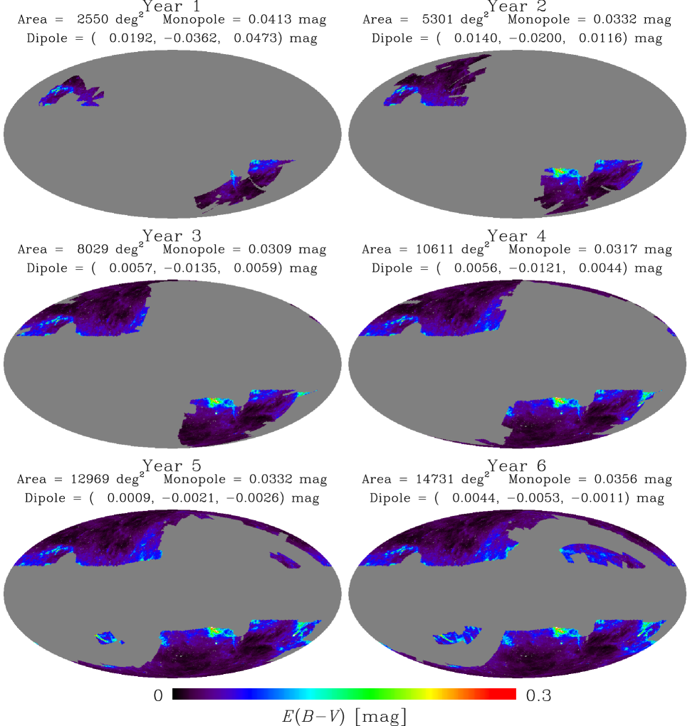
Figure 11: Cumulative coverage of the SFD $E(B-V)$ reddening map in Galactic coordinates. $A_{V}\sim 3.1E(B-V)$ and $A_{\rm near-IR}\sim E(B-V)$. For each year, annotations list the area of sky covered, the monopole, $\langle E(B-V)\rangle$, and the three dipole components.

Maps of reddening or extinction are detailed but are subject to systematic errors. Most commonly used ones originate in observations of far-IR emission (e.g. Schlegel et al. 1998). Models are required to convert the emission to a dust column density, then into a reddening $E(B-V)$, then into extinction $A_{V}$, and finally to extinction at the desired wavelength $A_{\lambda}$. Factors that influence these steps are dust temperature and composition, the ratio of total to selective extinction $R_{V}$, and the reddening law $A_{\lambda}$/$A_{V}$ (see Fig. 13). All of these are known to vary as a function of line of sight, but it is common (sometimes necessary) to simply adopt standard mean values for $R_{V}$ and the reddening law. This means that there will be some imprint of extinction even on an IGL background that is constructed from extinction corrected source magnitudes. The imprint will be that of the errors in the extinction correction. The errors, $\sigma_{A_{V}}$, will not necessarily have the same pattern on the sky as the extinction itself, i.e. $\sigma_{A_{V}}\neq\epsilon A_{V}$, where $\epsilon\ll 1$.

The example of the SFD extinction maps used here shows that extinction introduces a non-negligible diffuse dipole component, although it may differ in some detail from other Galactic extinction maps (e.g. Schlafly & Finkbeiner 2011; Planck Collaboration et al. 2014; Delchambre et al. 2023) and their wavelength dependence (e.g. Predehl & Schmitt 1995; Draine 2011). In what follows we introduce methodology to remove the dipole contribution from extinction (in the limit of low extinction, $A_{V}\ll 1$) independent of any estimated extinction map.

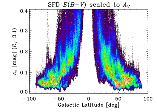
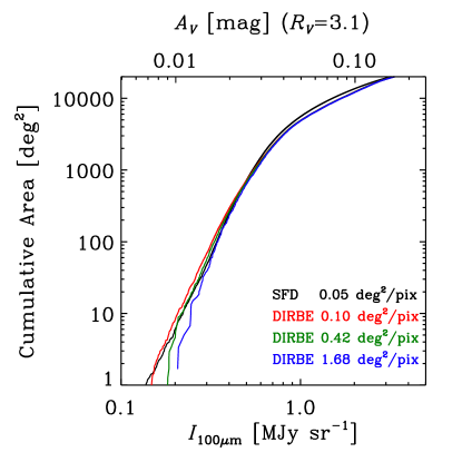
Figure 12: Left: $A_{V}$ as a function of Galactic latitude derived by converting SFD $E(B-V)$ results using $R_{V}=3.1$. The color excess (reddening) is $E(B-V)=(B-V)_{\rm observed}-(B-V)_{\rm intrinsic}$ and $R_{V}=A_{V}/E(B-V)$. Right: The cumulative area where the SFD extinction is less than $A_{V}$ or where the COBE/DIRBE 100 $\mu$m intensity (shown at 3 resolutions) is less than $I_{100\ \mu{\rm m}}$.

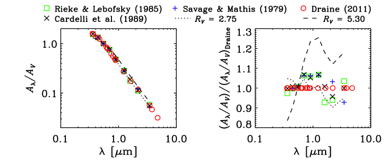
Figure 13: Left: Galactic extinction laws as reported by Draine (2011) (red $\circ$), Cardelli et al. (1989) (black $\times$), Rieke & Lebofsky (1985) (green $\square$), and Savage & Mathis (1979) (blue $+$). The dotted and dashed lines are the Cardelli et al. (1989) evaluated for $R_{V}=2.75$ and 5.30, respectively. Right: The same extinction laws are plotted normalized to the Draine (2011) extinction law to show that differences of several percent exist, and that variations of $\gtrsim 10\%$ can arise from $R_{V}$ variations.

4.4.2 Managing the extinction contributions

While the Galactic extinction can interfere with probing the intrinsic IGL dipole, its interference can be removed with the method proposed in this section. Let us say that the extinction correction, $A_{\nu}\ll 1$, is known to within $\sigma_{A}$. Then, after the extinction correction the flux in Eq. (7) becomes:

$$\tilde{I}_{\nu}(l,b)=\left[1-0.4\,(\ln{10})\left(\frac{\sigma_{A}}{A}\right)A_{\nu}\right]I_{\nu}(l,b)\equiv I_{\nu}(l,b)+\Delta I_{\nu}(l,b).$$ (11)

If no extinction corrections are made then one should read $\sigma_{A}=A$. This leads to the extinction uncertainty contribution to the measured IGL of

$$\Delta I_{\nu}(l,b)=\pm 0.92\left(\frac{\sigma_{A}}{A}\right)A\,I_{\nu}(m_{0},m_{1}){|_{(l,b)}}\,.$$ (12)

We now write $A\equiv\langle A\rangle+\delta A,I\equiv\langle I\rangle+\delta I$. Assuming that the extinction map in Fig. 12 has a dipole $\boldsymbol{D}_{A}$ we can write taking $\sigma_{A}/A=$const across the sky leads to the following uncertainty in the IGL dipole, Eq. (12), from extinction corrections

$$\begin{split}\tilde{\boldsymbol{d}}_{\nu}=\leavevmode\nobreak\ &\boldsymbol{d}_{\nu}\left[1-0.92\left(\frac{\sigma_{A}}{A}\right)\langle A_{\nu}\rangle\right]\\ &-0.92\left(\frac{\sigma_{A}}{A}\right)\boldsymbol{D}_{A}\langle I_{\nu}\rangle+O[{\rm dipole}(\delta A\,\delta I)]\,.\end{split}$$ (13)

Here $D_{A}$ is the dipole of the extinction map to be evaluated from the selected sky region in Fig. 12 (left). The spherical harmonic expansion is defined via: $I_{\nu}=\sum_{\ell m}d_{\ell m}Y_{\ell m}\;;\;A_{\nu}=\sum_{\ell m}D_{\ell m}Y_{\ell m}$. Over the full sky higher-$\ell$ harmonics do not couple to lower-$\ell$ ones. The extinction component of the dipole due to Eq. (12) decreases with wavelength ($\propto\lambda^{-2-\alpha_{\nu}}$) and, very generally, has a very different dependence on $\lambda$ from that of the IGL, $d_{\nu}$, shown in Fig. 2. This should enable component separation in Eq. (11).

If Eq. (13) is valid then the task of minimizing the extinction contribution to the probed IGL dipole is reduced to: 1) finding a region large enough to contain many galaxies [Table 1 in Kashlinsky & Atrio-Barandela (2022) shows that $N_{\rm gal}\gtrsim$1000$$–$2000$ deg² could be enough] that has small $\langle A_{\nu}\rangle$ and 2) where $D_{A}$ is sufficiently close to zero. For the Euclid bands the dimensionless IGL dipole is $(3-\alpha_{\nu})V/c\simeq 0.5\%$ if the measured CMB dipole is entirely kinematic (if not, then it would be ${\simeq}\,0.5\%V/V_{\rm CMB})$. Hence in the absence of further corrections discussed below, one would want to select the sky regions with $D_{A}/\langle A\rangle\lesssim 0.2(\sigma_{A}/A)^{-1}$ in $I_{\scriptscriptstyle\rm E}$, and significantly more relaxed in $H_{\scriptscriptstyle\rm E}$, in order to probe, in each of the bands, the IGL dipole with the expected dimensionless amplitude of ${\simeq}\,0.5\%$ per Fig. 23. The above hinges on three assumptions: 1) $D(\delta I\delta A)\ll\langle I\rangle D_{A},\langle A\rangle d_{\nu}$, 2) $\langle A\rangle,A\ll 1$, and 3) the coupling with higher $\ell$-order terms can be neglected (for now). Choosing a region where $D_{A}$ is minimal can be accomplished by selecting regions of the sky where $E(B-V)$ is roughly constant. Figure 11 illustrates that while the total sky observed by Euclid after any year contains a dipole, selection of an area of sky with near constant $E(B-V)$ can reduce the dipole amplitude by roughly an order of magnitude.

However, a more efficient technique would work as follows: Fig. 12 shows that the additive term, when multiplying $\boldsymbol{d}_{\nu}$ in the RHS of Eq. (13), is $0.92\langle A_{\nu}\rangle\ll 1$ and can be neglected. It further affects only the precise conversion of the dipole into the velocity amplitude (at less than a few percent level), not its direction. Assuming that the last term on the RHS is negligible, a firmer way to eliminate the extinction terms in Eq. (13) would be to 1) divide the large Euclid galaxy sample into two groups with very different spectral/morphological properties and 2) use one to eliminate the extinction dipole in the other. For example, if we define a subsample “a” with, say $\alpha_{\nu}^{\rm a}\gtrsim 1$, and magnitude range $m_{0}^{\rm a}<m<m_{1}^{\rm a}$, one would get for its dipole

$$\frac{\tilde{\boldsymbol{d}}_{\nu}^{\rm a}}{\langle I_{\nu}^{\rm a}\rangle}=(3-\alpha_{\nu}^{\rm a})\frac{\boldsymbol{V}}{c}-0.92\boldsymbol{D}_{A}(\lambda)\,,$$ (14)

and similarly for the main sample “b”. Then subtracting the two would lead to the residual wavelength-dependent dipole from extinction corrections determined as

$$\begin{split}\boldsymbol{D}_{A}(\lambda)=&\frac{(0.92)^{-1}}{(\alpha_{\nu}^{\rm b}-\alpha_{\nu}^{\rm a})}\\ &\times\left[(3-\alpha_{\nu}^{\rm a})\frac{\tilde{\boldsymbol{d}}_{\nu}^{\rm b}}{\langle I_{\nu}^{\rm b}(m_{0}^{\rm b},m_{1}^{\rm b})\rangle}-(3-\alpha_{\nu}^{\rm b})\frac{\tilde{\boldsymbol{d}}_{\nu}^{\rm a}}{\langle I_{\nu}^{\rm a}(m_{0}^{\rm a},m_{1}^{\rm a})\rangle}\right]\,.\end{split}$$ (15)

Whereas the wavelength-independent Compton–Getting velocity term is given by

$$(\alpha_{\nu}^{\rm b}-\alpha_{\nu}^{\rm a})\frac{\boldsymbol{V}}{c}=\boldsymbol{\Delta}_{\rm ab}\equiv-[\boldsymbol{{\cal U}}_{\rm a}-\boldsymbol{{\cal U}}_{\rm b}]\,,$$ (16)

where we further defined

$$\boldsymbol{{\cal U}}_{a,b}\equiv\frac{\tilde{\boldsymbol{d}}_{\nu}^{\rm a,b}}{\langle I_{\nu}^{\rm a,b}(m_{0}^{\rm a,b},m_{1}^{\rm a,b})\rangle}$$ (17)

to be used later. Note that the rms in Eq. (16) depends on the relative difference in $\alpha_{\nu}$ for the subsamples, rather than the absolute Compton–Getting amplification, $(3-\alpha_{\nu})$.

The values of $\boldsymbol{D}_{A}$ determined empirically here will help verify the accuracy of the Euclid extinction corrections. The errors resulting from this procedure are discussed in the next section using simulated Euclid catalogs. Naively speaking the statistical error on $D_{A}$ determined here from sample “b” would be $\sigma_{D_{A}}\sim D_{A}({N^{b}_{\rm gal})}^{-0.5}$.

We will have plenty of galaxies to do this per Table 1 of Kashlinsky & Atrio-Barandela (2022) and we want to choose subsample galaxies with, say, $I_{\scriptscriptstyle\rm E}-Y_{\scriptscriptstyle\rm E}<0$, $Y_{\scriptscriptstyle\rm E}-J_{\scriptscriptstyle\rm E}<0$, $J_{\scriptscriptstyle\rm E}-H_{\scriptscriptstyle\rm E}<0$ (in the observer frame) so that their IGL has positive $\alpha_{\nu}$, ideally closer to $\alpha_{\nu}^{\rm RJ}=2$ and $m_{0}$ faint enough to ensure that the dipole from the clustering component is small. Bisigello et al. (2020) show in their Figs. 6 and 7 that one can choose a substantial subsample of such galaxies. Since $I_{\nu}/\nu^{3}$ is Lorentz-invariant for each subsample its $\alpha_{\nu}$ is independent. Hence we can select subsamples with a significantly positive $\alpha_{\nu}$ from $I_{\scriptscriptstyle\rm E}$ to $H_{\scriptscriptstyle\rm E}$ bands and the main sample from galaxies with $\alpha_{\nu}$ substantially negative to compensate for the reduction in the overall $N_{\rm gal}$. Then we would choose the optimal $(m_{0}^{\rm sub},m_{1}^{\rm sub},m_{0},m_{1})$ to enable sufficient reduction in the dipole from clustering. Then use Eq. (16) and propagate the errors; with this in mind choose areas where $\tilde{d}_{\nu}$ (and $D_{A}$) are minimal. The resultant velocity, Eq. (16), must be the same when derived at all bands and the absorption dipole, $\boldsymbol{D}_{A}$ must point in the same direction and have the corresponding wavelength dependence decreasing with $\lambda$. This technique can be straightforwardly generalized to more subsamples with sufficiently different $\alpha_{\nu}$.

4.5 Accounting for the Earth’s orbital motion

The overall cosmological information was not yet available when the Compton–Getting effect was introduced almost 100 years ago as a way to probe the orbital motion of the Earth from cosmic ray observations (Compton & Getting 1935). The motivation is reversed here, but the well-known now Earth’s orbital motion is important to account for in any precision measurement.

Dipole measurements having ${\rm S/N}\gtrsim 10$ will be sensitive to (require correction for) the Earth’s (or spacecraft’s) orbital motion around the Sun at $V_{\oplus}\sim 30$ km s^-1. Mapping the data in a coordinate system that rotates to keep the Sun fixed [i.e. $(l_{\rm ecl}-l_{\sun},b_{\rm ecl})$ rather than $(l_{\rm ecl},b_{\rm ecl})$], can be used to determine the “Solar anisotropy” (e.g. Abbasi et al. 2012). In these coordinates the dipole can be fit, and then its brightness can be subtracted from each of the observations as mapped into a standard fixed coordinate system. In principle $(V_{\oplus}/c)\cos\Theta$ is already known, but this fitting provides an empirical measure of $\langle I\rangle$, which is needed for the subtraction. For Euclid this dipole is poorly sampled in Year 1 because all observations are towards the ecliptic poles, perpendicular to the Earth’s orbital motion dipole. However, for the same reason, the effect of this dipole will be correspondingly small in the Year 1 data. As the years progress and lower ecliptic latitudes are observed, sensitivity to the Solar anisotropy dipole increases. In this fixed-Sun coordinate system, the cosmological kinematic dipole on the sky will be a noise term that averages down for Euclid as more sky is sampled.

A more ideal solution is to modify dipole fitting routines (e.g. HEALPix remove_dipole) to include input specifying the time (or Solar elongation) of observation for each pixel and then subtract off the “Solar anisotropy” dipole as part of the fitting. In this case the fitting does not involve any additional free parameters, since the time (or Solar elongation) of the observations is a known quantity.

4.6 Photometry and magnitudes

Because galaxies are extended sources without cleanly defined edges, there are multiple ways to define the magnitude of a galaxy. Standard techniques include using aperture photometry within a radius set by the shape of the galaxy profile (e.g., Petrosian photometry), and fitting a generic profile shape to galaxies to measure something akin to a total magnitude [such as the CModel magnitudes developed by the Sloan Digital Sky Survey (Abazajian et al. 2004), and being used by the Hyper Suprime-Cam survey and the Rubin Observatory (Bosch et al. 2018)]. Such measurements will have Malmquist-like biases (i.e., where more faint galaxies scatter into the sample at the faint magnitude limit than the converse), which will depend on the sources of noise. If those sources of noise are not symmetric across the sky, this could imprint a false dipole moment into the inferred magnitude range. Given that the Euclid Wide Survey will have quite uniform coverage, and the location of Euclid at L2 means that the imaging depth should have little temporal variation, we anticipate that this will be a subdominant effect in the IGL dipole measurement, but we will have to measure it. The sky background of the measurements will not be uniform across the sky, adding to the noise of the galaxy photometry, and possibly leading to additional systematic errors. This varying sky background is dominated by zodiacal light, with a possible contribution at low Galactic latitudes from reflected starlight from diffuse dust in the Milky Way (optical cirrus), although the latter is again likely to be subdominant.

The availability of multi-band measurements of our galaxies allows us to carry out the measurements of the dipole from multiple independently defined subsamples, which should allow us to test the robustness of the results to many of the systematic errors we have described in this paper. In particular, we envision measuring the dipole on subsets of galaxies divided in the following ways:

• Dividing up the galaxies into different regions of color-color space, selected to identify galaxies at different (photometric) redshifts and different physical properties, and measuring the dipole for each;

• Dividing the galaxies into bins of magnitude;

• Dividing the sky by the season or year in which each patch was observed, to test for systematic biases in photometric zeropoints with time or position of the spacecraft;

• Dividing the galaxy sample by the morphology of the galaxy, as measured, e.g., by Sérsic index.

Seeing consistent dipoles among all these divisions of the data will give us confidence in the robustness of the results, and will allow us to constrain any residual systematic effects.

4.7 Systematic corrections

The dipole from the configuration by Eq. (7) will have additional contribution arising due to the Galaxy participating with the bulk motion $\Delta m=-(2.5\operatorname{log_{10}}{\rm e})[1-\beta(m)]\frac{V}{c}\cos\Theta$ for CIB sources with SED $f_{\nu}\propto\nu^{-\beta}$ (Ellis & Baldwin 1984; Itoh et al. 2010). The correction to the dipole from this effect can be evaluated by modifying the upper and lower limits on the integration in Eq. (3). Since $V\ll c$ the dipole due to Eq. (1) will be modified by the $m_{0}$, $m_{1}$ variation to

$$\boldsymbol{d}_{\nu}(m_{0}<m<m_{1})=[(3-\alpha_{\nu,m_{0}<m<m_{1}})+{\rm d}\alpha_{\nu}]\frac{\boldsymbol{V}}{c}\langle I_{\nu}(m_{0}<m<m_{1})\rangle\,,$$ (18)

with

$${\rm d}\alpha_{\nu}=Q_{\nu}(m_{1})[1-\langle\beta(m_{1})\rangle]-Q_{\nu}(m_{0})[1-\langle\beta(m_{0})\rangle]\,,$$ (19)

where we have defined

$$Q_{\nu}(m)\equiv\frac{\frac{{\rm d}I_{\nu}}{{\rm d}m}|_{m}}{\langle I_{\nu}(m_{0}\!\!<\!\!m\!\!<\!\!m_{1})\rangle}\,.$$ (20)

It was argued that the correction $d\alpha_{\nu}$ in general is small (Kashlinsky & Atrio-Barandela 2022), but here it must be evaluated explicitly for the Euclid configurations. This correction will affect only the (systematic) conversion of the measured IGL dipole into the effective velocity amplitude.

Figure 14 shows the values of $Q_{\nu}(m_{0})$ and $Q_{\nu}(m_{1})$ for the range of magnitudes defined by Eqs. (9) and (10) at the four Euclid bands with the vertical axis deliberately plotted to compare with the expected near-IR Compton–Getting amplification of $(3-\alpha_{\nu})\simeq 4.5$–$5.5$ at these bands. We used the latest JWST observations of galaxy counts shown in Fig. 5. The expected overall contribution, $\Delta\alpha_{\nu}$, after accounting for the SED/color terms, $\bar{\beta}$, will be incorporated from Euclid simulations in the next section.

Figure 14: The values of $Q_{\nu}(m_{0})$ (Eq. 20) vs. $\lambda$ are shown with filled circles and $Q_{\nu}(m_{1})$ with open circles at the Euclid four bands using the observed JWST galaxy counts from Windhorst et al. (2023). The values of $(m_{0},m_{1})$ were selected per Eqs. (9) and (10). The displayed vertical range reflects the Compton–Getting amplifications, $(3-\alpha_{\nu})\sim 4$–$5.5$, reachable here.

The Euclid Wide Survey will have measurements at an effective $\lambda$, within the four filters, from which we will need to reconstruct the genuine high-precision $I_{\nu}$, Eq. (3) and its derivative, $\alpha_{\nu}$ together with their uncertainties. This is discussed and quantified later in Sect. 5.3. To aid with this we will have photometric $z$ for the entire sample and spectroscopic $z$ for many of them. In particular, as discussed in Euclid Collaboration: Scaramella et al. (2022); Laureijs et al. (2011) we would expect upward of $5\times 10^{6}$ galaxies with spectroscopic redshifts already in Year 1 providing a good sample for such estimates.

4.8 Photometric zero points

A precision measurement of the intrinsic dipole in galaxy counts requires precision photometric calibration over the full survey footprint. Euclid’s photometric calibration is good, but is not perfect, and any dipole component in the error in photometric calibration will translate directly into a false dipole signature. In particular, the dipole moment of a calibration error $\Delta m_{\rm dipole}$ will behave exactly like that described in Eq. (18), and the (false) bulk motion $V_{\rm false}$ inferred from this dipole is given by

$$\Delta m_{\rm dipole}=-(2.5\operatorname{log_{10}}{\rm e})[1-\beta(m)]\frac{V_{\rm false}}{c}.$$ (21)

For reasonable values of $\beta$, a $V_{\rm false}$ of 300 km/s (i.e., the amplitude of the signal we are trying to measure) would correspond to a 0.5% $\Delta m_{\rm dipole}$.

The Euclid Wide Survey strategy is described in detail in Euclid Collaboration: Scaramella et al. (2022), and the calibration of the photometric system is described in Euclid Collaboration: Schirmer et al. (2022). Most of the roughly $15\,000$ deg² of sky will be observed only once, meaning that strategies that use overlaps to tie photometric calibration together (e.g. Padmanabhan et al. 2008; Burke et al. 2018) will be of only limited use. Rather, every 25–35 days, Euclid will observe a self-calibration field within its continuous viewing zone near the north ecliptic pole, to redetermine the photometric calibration of the bands. Section 6.3.3 of Euclid Collaboration: Schirmer et al. (2022) predicts that temporal changes in the photometric calibration will be determined to an accuracy of 1–2 milli-mag, although the formal requirement on the calibration is far looser, 1.5% for the NISP instrument. It is less clear what the dipole moment across the sky of this calibration error will be. If the calibration error is uncorrelated across the sky in each field that is observed, the dipole will be of order the error per independent calibrated patch, divided by the square root of the number of patches. In this context, the number of patches is determined by how often the calibration is checked. This means $\sim 12$ patches per year of survey operations. This would suggest a residual dipole error due to calibration uncertainties that is small relative to the expected signal. However, if the calibration errors are position-dependent in some way (e.g., somehow matching the scanning pattern of Euclid, or dependent on the angular separation of any given field from the self-calibration field), the systematic error on our measurement may be considerably larger, and we will need to work with the Euclid calibration team to explore the systematic calibration errors.

We anticipate that any calibration errors, if they are due to, e.g., time-dependent changes in Euclid’s throughput, will be correlated between Euclid’s different bands. This means that comparisons of the inferred dipole between bands is unlikely to be a panacea to such effects. Similarly, calibration problems will be likely to affect the photometry of different galaxy populations in the same way, so splitting galaxies by, e.g., measured color, will not be informative.

5 Applying to the upcoming Euclid Wide Survey

5.1 Evaluating overall statistical uncertainties

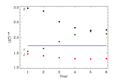
Figure 15: Variation of the Poisson errors over the cumulative sky coverage of Fig. 11 as a function of mission years. Black, green and red correspond to the $X$, $Y$ and $Z$ direction cosines. The blue straight line shows $\langle X_{i}^{2}\rangle^{-1/2}=\sqrt{3}$, the value for a full sky coverage.

The statistical (Poisson) errors on each dipole component are a function of the number density of galaxies and the area of the sky covered by the data. To compute these statistical uncertainties for the magnitude ranges of Eqs. (9) and (10) we used the number density of galaxies from the JWST counts, denoted by red asterisks in Fig. 10. The number densities of galaxies on an area of $2550$ deg², the size of the observed region in the first year of integration were $N_{\rm gal}=[313,270,313,362]\times 10^{6}$ for the Euclid $I_{\scriptscriptstyle\rm E}$, $Y_{\scriptscriptstyle\rm E}$, $J_{\scriptscriptstyle\rm E}$, and $H_{\scriptscriptstyle\rm E}$ filters, respectively. The uncertainty in each component of the dipole $d_{\nu,i}$ is

$$\sigma_{i}=\frac{1}{\sqrt{\langle X_{i}^{2}\rangle}}N_{\rm gal}^{-1/2}\,,$$ (22)

where the index $i=(X,Y,Z)$ denotes the components of the dipole, $N_{\rm gal}$ is the total number of galaxies and $\langle X_{i}^{2}\rangle$ is the square of the $i$th component of the direction cosine averaged over the observed region (Atrio-Barandela et al. 2010; Kashlinsky & Atrio-Barandela 2022).

In Fig. 15 we plot $\langle X_{i}^{2}\rangle^{-1/2}=\sigma_{i}N_{\rm gal}^{1/2}$, which measures the variation of the Poisson errors due to the increment of the sky coverage by mission years shown in Fig. 11. Black, green and red dots show this magnitude for the $X$, $Y$, and $Z$ direction cosines, respectively. The blue solid line shows the same magnitude for a full sky coverage. In the first two years, the mission will observe preferentially close to the ecliptic poles and the $Y$ and $Z$ components are reasonably well measured. At the end of the mission, the $Z$ component will have the smallest error bar since the areas near the Galactic poles will be the regions best observed by Euclid. A different scanning strategy will lead to different errors. Notice that, while the error on $Z$ is smaller than $\sqrt{3}$, the other two components are measured with an error larger than $\sqrt{3}$ and the error on the dipole amplitude is, as expected, larger than for a full sky coverage; see Atrio-Barandela et al. (2010) for extensive discussion.

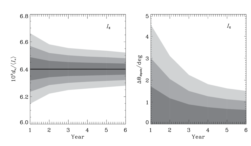
Figure 16: Regions of 68% (dark grey), 95% (middle grey) and 99.75% (light grey) confidence level measured from the region of the sky after 1 to 6 years of observations with the $I_{\scriptscriptstyle\rm E}$ band. The left panel shows the uncertainty of the dipole amplitude, with the horizontal thick line indicating the expected amplitude for a velocity of $V=370$ km s^-1. The right panel shows the uncertainty on the CMB dipole direction determination. The dipole is assumed to be in the direction of the Solar dipole, $(l,b)=(263\aas@@fstack{\circ}85,48\aas@@fstack{\circ}25)$ in Galactic coordinates.

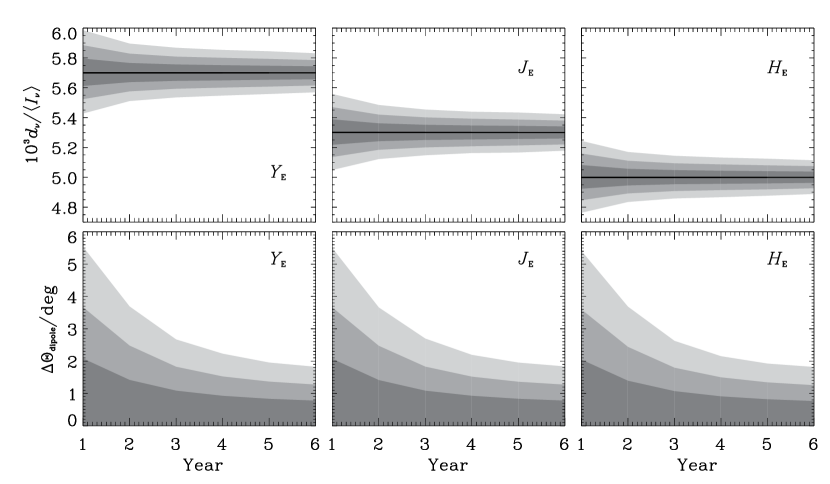
Figure 17: Same as in Fig. 16 for the NISP filters. In the top three panels the uncertainty of the dipole amplitude is represented, with the horizontal thick line showing the expected amplitude. The lower panels show the uncertainty on the CMB dipole direction. Left, middle and right panels correspond to the $Y_{\scriptscriptstyle\rm E}$, $J_{\scriptscriptstyle\rm E}$ and $H_{\scriptscriptstyle\rm E}$ NISP Euclid filters, as indicated.

In Figs. 16 and 17 we present the expected confidence contours on the dipole amplitude and direction for the VIS and NISP Euclid Wide Survey data obtained from the Poisson errors $\sigma_{i}$. We assumed the dipole is in the direction of the CMB Solar dipole $(l,b)=(263\aas@@fstack{\circ}85,48\aas@@fstack{\circ}25)$. For each filter and year of observation we generated $10^{5}$ Gaussian distributed random errors around the CMB measured components $(d_{\nu,X},d_{\nu,Y},d_{\nu,Z})$. We computed the random dipole amplitudes and their angular separations with respect to the CMB dipole direction. The confidence levels shown in Fig. 16 were defined as the regions that enclose the 68%, 95%, and 99.75% of all simulated amplitudes and directions. The left panel displays the contours in the amplitude and the right panel in the direction. The darkest and lightest colors correspond to the 1 and 3 $\sigma$ contours, respectively. The horizontal line in the left panel represents the dipole amplitude with the Solar System moving at $V=V_{\rm CMB}=370$ km s^-1 with respect to the CMB frame. In Fig. 17, the top three panels represent the dipole amplitude and the bottom three panels the dipole direction and their uncertainties with the same notation than in Fig. 16. The left, center and right panels correspond to the NISP filters $Y_{\scriptscriptstyle\rm E}$, $J_{\scriptscriptstyle\rm E}$, and $H_{\scriptscriptstyle\rm E}$, as indicated. The $(3-\alpha_{\nu})(V/c)$ coefficients used to estimate the statistical significance are given later by Eq. (33) in Sect. 5.3 below.

If the CMB dipole is entirely kinematic the statistical significance will be dominated by the $Z$ component as shown in Fig. 15 due to a larger number of observations close to the Galactic poles. As the figure shows, for the assumed cumulative sky coverage, the $Y$ component is more efficiently probed in the first two years, when the observations are closer to the ecliptic poles. The $X$ component will always be ill sampled and since its value is close to zero, its ${\rm S/N}$ will be always negligible.

The number of galaxies given separately by Eqs. (9) and (10) and the amplification factor with respect to the CMB dipole are different for each of the Euclid bands although the overall ${\rm S/N}$ is very similar for the three NISP filters. The measured amplitude and direction on each of the filters must be consistent with the uncertainties given in Figs. 16 and 17. Larger differences will be an indication of systematics from extinction correction, star contamination, etc., if remaining in the data. For instance, extinction will be a stronger contaminant for $I_{\scriptscriptstyle\rm E}$ than for the $H_{\scriptscriptstyle\rm E}$  filter. In the following section we use a galaxy catalog obtained from the Euclid Flagship Mock Galaxy Catalogue to apply the methodology developed in the previous section for eliminating extinction dipole contributions remaining in the Euclid Wide Survey.

The high precision measurement of the IGL/CIB dipole would allow subdividing the galaxy sample by narrow magnitude bins within the range of Eqs. (9) and (10) in order to probe any dependence of the velocity on these parameters. Likewise, given the expected large sample of the Euclid Wide Survey galaxies with spectroscopic redshifts, one can divide the galaxies by $z$ in order to probe the behavior of $V$ in different $z$-shells.

5.2 Uncertainties on the IGL/CIB kinematic dipole after extinction corrections

To incorporate the proposed above method for removing residual dipole from extinction corrections we used the Euclid Flagship Mock Galaxy Catalogue (version 2.1.10) (Castander et al., in prep.) This catalog contains photometry in the Euclid bands (and many other UV – near-IR bands), and has major emphasis on modelling the clustering and shapes of galaxies in the range $0<z<3$, as needed for dark energy studies. This catalog does include Galactic extinction and could be used to calculate $\boldsymbol{D}_{A}$, but its ${\sim}\,4.8$ billion sources are distributed only over ${\sim}\,$5000$$ deg² in the general direction of the north Galactic pole. We used CosmoHub (Carretero et al. 2017; Tallada et al. 2020) to download a 1/128th fraction of the catalog (${\sim}\,38$ million galaxies) including photometry (with extinction applied) at (Subaru) $b$, (Euclid) $I_{\scriptscriptstyle\rm E}$, $Y_{\scriptscriptstyle\rm E}$, $J_{\scriptscriptstyle\rm E}$, $H_{\scriptscriptstyle\rm E}$, and (WISE) W1 and W2 bands. Ancillary parameters downloaded were the galactic coordinates $(l,b)$, the value of the color excess [$E(B-V)$], and the redshift ($z$) of each source. The downloaded catalog contains 38 million galaxies, a factor of ${\sim}\,1.6$ larger than expected from the observed galaxy counts and the HRK reconstruction. This is a known issue that was communicated to Euclid by K. Helgason (private communication), but has no consequences for our goal here of testing the separation of galaxies by the resultant $\alpha_{\nu}$ (the logarithmic slope of the CIB with $\nu$). The catalog provides individual apparent galaxy fluxes, $F$, in each band in units of erg Hz^-1 s^-1 cm^-2, which were also converted into AB magnitudes as $m=-2.5\operatorname{log_{10}}F-48.6$. We then select a conservative subset of galaxies satisfying simultaneously both Eqs. (9) and (10).

From the downloaded catalog we removed galaxies at VIS/NISP bands $m<m_{0}=19/18$ and $m>m_{1}=24.5/24$. From the overall sample covering total area $A$ sr at $m_{0}\leq m\leq m_{1}$ we computed the net CIB flux density in MJy sr^-1 as $I_{\nu}=\sum F_{i}/A$ at each frequency $\nu$ and used the data to evaluate its logarithmic derivative $\alpha_{\nu}$ between 0.4 and 5 $\mathrm{\SIUnitSymbolMicro m}$ for each subsequently selected subsample aiming to divide into at least two groups in Eq. (16). As discussed in the previous section this achieves two goals: 1) verifying the same $\boldsymbol{V}(\alpha)$ at each $\alpha_{\nu}$ as well as $\nu$ for every pair of sample+subsample, and 2) refining the overall $\boldsymbol{V}$ via $\chi^{2}$ from finer sample binning with each having more uniform $\alpha$.

We now turn to several specific examples of binning by the effective to apply the method to isolate and separate the extinction term from the kinematic IGL/CIB dipole. We define the effective slope between two adjacent Euclid wavelengths (1 and 2) for each Flagship catalog source contributing individual fluxes $F_{1,2}$ to IGL as

$$\beta_{1\rightarrow 2}\equiv\frac{\ln(F_{1}/F_{2})}{\ln(\lambda_{1}/\lambda_{2})}\,.$$ (23)

In the first example we select all sources in the 2 individual subsamples where each color satisfies: 1)

$$[\beta_{I_{\scriptscriptstyle\rm E}\rightarrow Y_{\scriptscriptstyle\rm E}},\beta_{Y_{\scriptscriptstyle\rm E}\rightarrow J_{\scriptscriptstyle\rm E}},\beta_{J_{\scriptscriptstyle\rm E}\rightarrow H_{\scriptscriptstyle\rm E}}]\leq\beta$$ (24)

for the extinction, and 2)

$$[\beta_{I_{\scriptscriptstyle\rm E}\rightarrow Y_{\scriptscriptstyle\rm E}},\beta_{Y_{\scriptscriptstyle\rm E}\rightarrow J_{\scriptscriptstyle\rm E}},\beta_{J_{\scriptscriptstyle\rm E}\rightarrow H_{\scriptscriptstyle\rm E}}]\geq\beta$$ (25)

for the IGL dipole.

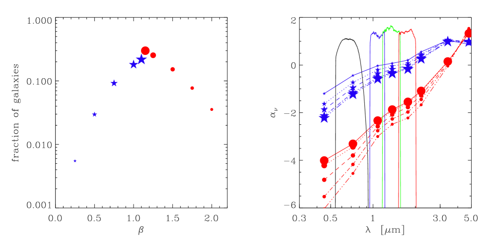
Figure 18: Blue asterisks mark selection according to Eq. (24), and red circles according to Eq. (25). The left panel shows the fraction of the Flagship catalog galaxies vs. $\beta$ according to Eqs. (24) and (25). Symbol size increases with the sample size. The right panel shows the resultant $\alpha_{\nu}$ vs. wavelength for the two subsamples following the notations in the left panel. The panel demonstrates the separability when Eq. (16) is applied at the marked Euclid bands of $I_{\scriptscriptstyle\rm E}$, $Y_{\scriptscriptstyle\rm E}$, $J_{\scriptscriptstyle\rm E}$, and $H_{\scriptscriptstyle\rm E}$.

Figure 18 (left) shows the fraction of galaxies vs. $\beta$ for each category in this case marked with red asterisks for Eq. (24) and blue circles according to Eq. (25). The plot shows that one could select samples of sufficient size in order to achieve high statistical accuracy when separating extinction contributions. The right panel of the figure shows the corresponding $\alpha_{\nu}$ for the IGL from sources in each subsample. This demonstrates a clear difference between the Compton–Getting dipole amplification in the two subsample as required for good separation according to Eq. (16). The figure illustrates the desirable separability of IGL by $\alpha_{\nu}$ and show that one robustly recovers $\Delta\alpha_{\nu}\equiv|\alpha_{\nu}^{a}-\alpha_{\nu}^{b}|\gtrsim 2$ at the Euclid four bands, which are marked in black ($I_{\scriptscriptstyle\rm E}$), blue ($Y_{\scriptscriptstyle\rm E}$), green ($J_{\scriptscriptstyle\rm E}$), and red ($H_{\scriptscriptstyle\rm E}$).

In Figs. 19–21 we present similar examples using alternate criteria for subsample selection. Subsample selections for Fig. 19 include only NISP colors (omitting the bluest, $I_{\scriptscriptstyle\rm E}$, band):

$$[\beta_{Y_{\scriptscriptstyle\rm E}\rightarrow J_{\scriptscriptstyle\rm E}},\beta_{J_{\scriptscriptstyle\rm E}\rightarrow H_{\scriptscriptstyle\rm E}}] \leq \beta\,,$$ (26)

$$[\beta_{Y_{\scriptscriptstyle\rm E}\rightarrow J_{\scriptscriptstyle\rm E}},\beta_{J_{\scriptscriptstyle\rm E}\rightarrow H_{\scriptscriptstyle\rm E}}] \geq \beta\,.$$ (27)

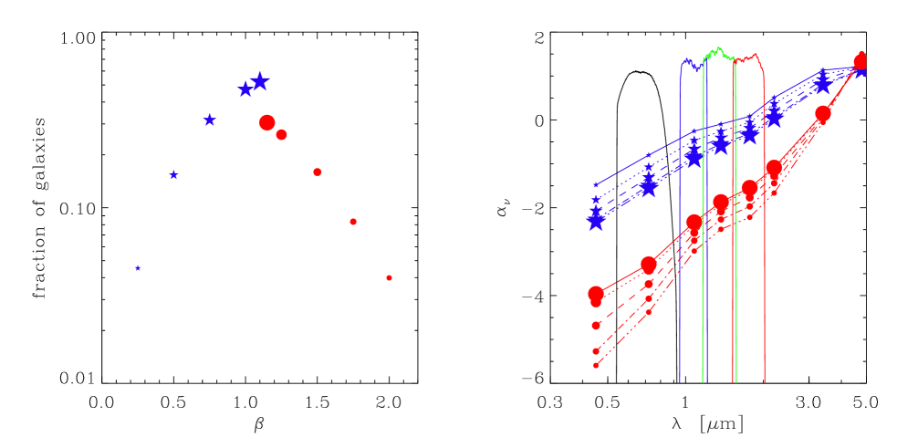
Figure 19: Blue asterisks mark selection according to Eq. (27), and red circles according to Eq. (27). The left panel shows the fraction of the Flagship catalog galaxies vs. $\beta$ according to Eqs. (27) and (27). Symbol size increases with the sample size. The right panel shows the resultant $\alpha_{\nu}$ vs. wavelength for the two subsamples following the notations in the left panel. The panel demonstrates the separability when Eq. (16) is applied at the marked Euclid bands of $I_{\scriptscriptstyle\rm E}$, $Y_{\scriptscriptstyle\rm E}$, $J_{\scriptscriptstyle\rm E}$, and $H_{\scriptscriptstyle\rm E}$.

Subsample selections for Fig. 20 omit the reddest, $H_{\scriptscriptstyle\rm E}$, band:

$$[\beta_{I_{\scriptscriptstyle\rm E}\rightarrow Y_{\scriptscriptstyle\rm E}},\beta_{Y_{\scriptscriptstyle\rm E}\rightarrow J_{\scriptscriptstyle\rm E}}] \leq \beta\,,$$ (28)

$$[\beta_{I_{\scriptscriptstyle\rm E}\rightarrow Y_{\scriptscriptstyle\rm E}},\beta_{Y_{\scriptscriptstyle\rm E}\rightarrow J_{\scriptscriptstyle\rm E}}] \geq \beta\,.$$ (29)

Figure 20: Blue asterisks mark selection according to Eq. (29), and red circles according to Eq. (29). The left panel shows the fraction of the Flagship catalog galaxies vs. $\beta$ according to Eqs. (29) and (29). Symbol size increases with the sample size. The right panel shows the resultant $\alpha_{\nu}$ vs. wavelength for the two subsamples following the notations in the left panel. The panel demonstrates the separability when Eq. (16) is applied at the marked Euclid bands of $I_{\scriptscriptstyle\rm E}$, $Y_{\scriptscriptstyle\rm E}$, $J_{\scriptscriptstyle\rm E}$, and $H_{\scriptscriptstyle\rm E}$.

For Fig. 21, we select all sources in the two individual subsamples where the $1\rightarrow 2$ color for each of the three pairs ($I_{\scriptscriptstyle\rm E}$,$Y_{\scriptscriptstyle\rm E}$), ($Y_{\scriptscriptstyle\rm E}$,$J_{\scriptscriptstyle\rm E}$), and ($J_{\scriptscriptstyle\rm E}$,$H_{\scriptscriptstyle\rm E}$) separately satisfies

$$\beta_{\rm 1\rightarrow 2} \leq {\rm median}(\beta_{\rm 1\rightarrow 2})\,,$$ (30)

$$\beta_{\rm 1\rightarrow 2} \geq {\rm median}(\beta_{\rm 1\rightarrow 2})\,.$$ (31)

Figure 21: Blue asterisks mark selection according to Eq. (31), and red circles according to Eq. (31). The left panel shows the fraction of the Flagship catalog galaxies vs. $\beta$ according to Eqs. (31) and (31). Symbol size increases from ($I_{\scriptscriptstyle\rm E}$,$Y_{\scriptscriptstyle\rm E}$), through ($Y_{\scriptscriptstyle\rm E}$,$J_{\scriptscriptstyle\rm E}$), to ($J_{\scriptscriptstyle\rm E}$,$H_{\scriptscriptstyle\rm E}$). The right panel shows the resultant $\alpha_{\nu}$ vs. wavelength for the two subsamples following the notations in the left panel. The panel demonstrates the separability when Eq. (16) is applied at the marked Euclid bands of $I_{\scriptscriptstyle\rm E}$, $Y_{\scriptscriptstyle\rm E}$, $J_{\scriptscriptstyle\rm E}$, and $H_{\scriptscriptstyle\rm E}$.

Now we can solve for $\boldsymbol{D}_{A}$ and $\boldsymbol{V}$ in Eqs. (15) and (16) and determine their uncertainties. Equation (16) is sensitive to the difference in $\alpha$’s between the “(a,b)” subsamples. Hence, to optimize the ${\rm S/N}$ for Eq. (16) we need to select 1) a more amplified subsample “a” (with more negative $\alpha_{\nu}^{a}$), then 2) select subsample “b” with much less negative $\alpha_{\nu}^{b}$, so ${\cal U}_{\rm b}^{2}\ll{\cal U}_{\rm a}^{2}$ (squares are since the uncertainties add in quadrature), while 3) keeping enough galaxies in the subsamples, so that 4) the final signal-to-noise ratio

$$({\rm S/N})_{\Delta_{\rm ab}}\simeq({\rm S/N})\left[\frac{|\Delta\alpha_{\nu}|}{(3-\alpha_{\nu}^{\rm total})}\;\;\sqrt{\frac{f_{\rm a}f_{\rm b}}{f_{\rm a}+f_{\rm b}}}\;\right]$$ (32)

will still be high enough. In this expression, $f_{\rm a}$ and $f_{\rm b}$ are the fractions of ${\rm a}$ and ${\rm b}$ galaxies to the total number of galaxies with $\alpha_{\nu}^{\rm a,b}$ being the spectral indices of their respective IGLs. Equation (32) shows that significant ${\rm S/N}$ can be achieved by dividing the galaxy population into distinct samples with very different $\alpha_{\nu}$ and the figures in this section show that several of these samples are possible. We note that this procedure will be required only if we determine, from the actual data, that the extinction dipole, Eq. (15), is significant in all the Euclid bands. If it turns out negligible, the method for correcting for the remaining extinction proposed here will not be required and we will proceed with the measurement per Eqs. (7) and (8) directly.

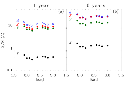
Figure 22: Statistical significance of the three dipole components and the dipole amplitude measured using the $I_{\scriptscriptstyle\rm E}$ data and assuming the CMB dipole template, Eq. (6). Black, green, red full circles correspond to the $X$, $Y$, and $Z$ dipole components; blue open circles to the overall dipole amplitude $d$. The left panel (a) shows the result after one year of integration and the right panel (b) at the end of the 6-year mission. The fraction of the total number of galaxies in samples a and b are, from left to right, $f_{\rm a}=[0.5,0.2,0.1,0.2,0.2,0.2,0.15,0.1,0.2]$ and $f_{\rm b}=[0.5,0.3,0.3,0.25,0.2,0.2,0.2,0.2,0.1]$, respectively. For other configurations the ${\rm S/N}$ will increase according to Eq. (32).

If the extinction dipole, Eq. (15), turns out to be important we will proceed as outlined in this section. This discussion suggests many possibilities to optimize the measurement after isolating the extinction. Equation (32) shows that this is achievable with the ${\rm S/N}$ loss of a factor of ${\sim}\,2$ if one concentrates on galaxy subsamples with $|\Delta\alpha_{\nu}|\sim 2$–3 while keeping the bulk of galaxies in both samples, so that $f_{\rm a},f_{\rm b}\sim 0.3$–0.5. Additionally, the measurement in the four Euclid bands with significantly varying extinction levels may lead to further clarity, since the $H_{\scriptscriptstyle\rm E}$ channel will have an order of magnitude lower extinction levels than $I_{\scriptscriptstyle\rm E}$.

As the worst-case scenario in terms of the extinction contribution we consider the application of the presented formalism to the $I_{\scriptscriptstyle\rm E}$ band. Figure 22 shows with full circles the ${\rm S/N}$ of the three IGL/CIB dipole components $(X,Y,Z)$ and the overall IGL/CIB dipole amplitude $d$ with open circles, for the first year and after six years of observations using the data of the $I_{\scriptscriptstyle\rm E}$ band alone and assuming $\boldsymbol{V}=\boldsymbol{V}_{\rm CMB}$. Since the dipole amplitude follows a $\chi^{2}$ distribution, we define the uncertainty as half the width of the interval enclosing the 68% confidence level. As indicated in Sect. 5.1 the best measured component is always $Z$ since Euclid will be observing preferentially around the Galactic poles, while the $Y$ component is better determined in the first two years of the mission, when the observations take place near the ecliptic poles. For the assumed dipole direction to be coincidental with the CMB dipole, the amplitude of the $X$ component is negligible so its statistical significance is always small; this would change if the observed CMB dipole has a non-kinematic component.

Dividing the galaxy sample into two equally sized subsamples with $|\Delta\alpha_{\nu}|\gtrsim 2$ we can measure in $I_{\scriptscriptstyle\rm E}$ alone the amplitude of the IGL/CIB dipole with ${\rm S/N}\gtrsim 15$ after the first year and $\gtrsim 30$ at the end of the mission. After six years of observation, the $Z$ dipole component is determined about a factor of two better than $Y$, dominating the statistical significance of the dipole amplitude, that is only a few percent better than $Z$. Depending on the value of $|\Delta\alpha_{\nu}|$ four or six different samples could be constructed and optimized from the actual data, so the statistical significance could additionally increase. Similar results hold for the NISP filters, resulting in a further increment of a factor of $2$. However, the statistical significance would be ${\rm S/N}>100$ if the extinction dipole is small at least at the longest wavelengths and does not need to be subtracted off from the data. Comparison of the measured IGL/CIB dipole subtracting and not subtracting the extinction dipole will further indicate the importance of this component at each frequency. Furthermore, juxtaposition between different frequencies will be a measure of systematic uncertainties. Large differences would indicate that extinction and/or other systematic uncertainties are present in the data and if such differences do not exist it will provide a strong vindication of the final result for the IGL/CIB dipole.

If the post-extinction-correction IGL/CIB maps at the different Euclid bands are found to be uncorrelated (e.g. the extinction dipoles, Eq. (15) are found to be widely different) one can potentially gain an improvement of up to a factor of 2 in the ${\rm S/N}$ over that shown in Fig. 22.

To conclude this section, we have shown explicitly the many combinations that can be selected by color between the various Euclid bands, in order to isolate the remaining extinction contribution and achieve the required IGL/CIB dipole measurement. Of course, when the data arrive they will be dissected in more possible ways to fine-tune and optimize the measurement, and still more combinations of colors may be considered. The formalism developed here for isolating and removing the extinction contributions to the CIB dipole is mathematically precise and independent of any particular extinction model with the SFD maps used merely as an example of what the extinction dipole may look like.

5.3 Reducing systematic amplification uncertainties

Finally we concentrate on the systematic corrections needed to translate accurately the IGL/CIB dipole, for a well determined direction, into the corresponding velocity amplitude. The corrections below affect all 3 components of the velocity vector equally, leaving the direction intact. We will reconstruct the IGL/CIB from counts, evaluate as accurately as possible the value of $\alpha_{\nu}$ across the Euclid spectrum, probe its dipole components and then deduce the effective velocity accounting for the systematics below.

Our task is to translate the measured CIB dipole into the equivalent velocity and compare to $V_{\rm CMB}=370$ km s^-1 in the precisely known direction $(l,b)_{\rm CMB}=(263\aas@@fstack{\circ}85\pm 0\aas@@fstack{\circ}1,48\aas@@fstack{\circ}25\pm 0\aas@@fstack{\circ}04)$ (Hinshaw et al. 2009). For precision measurement we must translate the measured dipole amplitude into the equivalent velocity with required accuracy when selecting galaxies with $m\geq m_{0}$ (to eliminate the contribution to dipole from galaxy clustering). Figure 23 shows the dimensionless Compton–Getting amplified IGL dipole amplitude for $V=370$ km s^-1 expected for Flagship 2.1 galaxies satisfying simultaneously Eqs. (9) and (10). Specifically, if the CMB dipole is purely kinematic, one would recover at the four Euclid bands, $I_{\scriptscriptstyle\rm E}$, $Y_{\scriptscriptstyle\rm E}$, $J_{\scriptscriptstyle\rm E}$, and $H_{\scriptscriptstyle\rm E}$

$$(3-\alpha_{\nu})\frac{V_{\rm CMB}}{c}=[6.4,5.7,5.3,5.0]\times 10^{-3}\,.$$ (33)

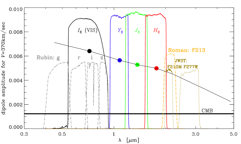
Figure 23: The solid line shows the dimensionless IGL/CIB dipole from the Flagship2.1 catalog in the configuration used here combining the configuration given by Eqs. (9) and (10). The figure assumes that $V=V_{\rm CMB}$, with the CMB dimensionless dipole marked with the thick horizontal line. The Euclid filters are shown with the filled circles showing the values at their nominal wavelengths. The Roman F213 filter covering photons just outside of the $H_{\scriptscriptstyle\rm E}$ NISP band, JWST F210M and F277W filters also near and longward of the $H_{\scriptscriptstyle\rm E}$ band, and Rubin’s $g$, $r$, $i$, and $z$ filters are also shown. With this additional coverage the value of $\alpha_{\nu}$ can be evaluated to good accuracy.

The systematic correction, $\Delta\alpha_{\nu}$ discussed in Sect. 4, if uncorrected for would lead to velocity amplitude difference of $\Delta V/V\simeq d\alpha_{\nu}/(3-\alpha_{\nu})$, or

$$\frac{\Delta V}{V}=\frac{Q_{\nu}(m_{1})[1-\langle\beta(m_{1})\rangle]-Q_{\nu}(m_{0})[1-\langle\beta(m_{0})\rangle]}{(3-\alpha_{\nu})}\,.$$ (34)

For the Flagship2.1 catalog the relative magnitude of this systematic correction, $\Delta V/V$, was evaluated to be $[0.04,0.05,0.07,0.17]$ in the [$I_{\scriptscriptstyle\rm E}$, $Y_{\scriptscriptstyle\rm E}$, $J_{\scriptscriptstyle\rm E}$, $H_{\scriptscriptstyle\rm E}$ ] bands and is less than or comparable in magnitude to the correction due to Earth’s orbital velocity. It does not affect the direction of the dipole and when converting the measured IGL/CIB dipole into the equivalent amplitude for the velocity the magnitude of $d\alpha_{\nu}$ will be evaluated for each band directly from the Euclid galaxy data and incorporated into the overall amplification per Eqs. (18) and (34). Moreover, we can gauge the effects of $\alpha_{\nu}$ by considering the galaxy SED estimated by the photometric redshift fitting.

The derivative $\alpha_{\nu}$ may not be highly precise given the sparsity of points from Euclid’s four bands alone, particularly at $I_{\scriptscriptstyle\rm E}$ and $H_{\scriptscriptstyle\rm E}$. To more accurately compute $\alpha_{\nu}$, Eq. (2), in each of the four Euclid bands it would be useful to assemble a subset of the Euclid Wide Survey galaxies at wavelengths shorter than $I_{\scriptscriptstyle\rm E}$ and longer than $H_{\scriptscriptstyle\rm E}$ as e.g. shown in the figures in Sect. 5.2. From such a subsample we would evaluate the net IGL over the range of Euclid-selected magnitudes, Eqs. (9) and (10), and then evaluate its logarithmic derivative at $I_{\scriptscriptstyle\rm E}$ and $H_{\scriptscriptstyle\rm E}$. This can be achieved by using $ugriz$ data from various ground-based surveys that are providing complementary short wavelength data (see Euclid Collaboration: Scaramella et al. 2022), and using past Spitzer and future Roman data at longer wavelengths. The additional Roman data will be particularly useful here for accurately evaluating the Compton–Getting amplification at the $H_{\scriptscriptstyle\rm E}$ band. The data will be collected, even if over smaller area as currently envisaged, at F184 and F213 bands to magnitudes much deeper than the Euclid Wide Survey resulting in very rich sample of galaxies in the range of Eqs. (9) and (10) as discussed in Akeson et al. (2019).

The compilation of multiband galaxy photometry in the COSMOS field by the COSMOS2020 team (Weaver et al. 2022) can be used to measure typical values for $\alpha_{\nu}$ in the $I_{\scriptscriptstyle\rm E}$ and $H_{\scriptscriptstyle\rm E}$ bands. The COSMOS2020 compilation includes very deep multiband $YJHK_{s}$ imaging reaching $m>25$, $grizy$ photometry to 26–27 mag, and 3.6 and 4.5 $\mu$m to $m>25.5$ covering the 2 deg² COSMOS field. The COSMOS $K_{s}$ imaging has been homogenized and is considerably deeper than the 24 mag requirement over the full field. All the COSMOS2020 imaging is registered astrometrically to Gaia precision. Given the combination of sensitivity and precision available for the publicly available COSMOS2020 catalog, we will easily be able to construct galaxy counts for of order $200\,000$ $J$-detected galaxies reaching 24 mag in the $J$, $K_{s}$, 3.6 $\mu$m, and 4.5 $\mu$m bands (Fig.  11 of Weaver et al. 2022). We can go similarly deep blueward of the $I_{\scriptscriptstyle\rm E}$ band, allowing us to make a high-precision estimate of $\alpha_{\nu}$ in the Euclid $H_{\scriptscriptstyle\rm E}$ and $I_{\scriptscriptstyle\rm E}$ bands. The data from Spitzer at 3.6 nad 4.5 $\mathrm{\SIUnitSymbolMicro m}$ from e.g. Ashby et al. (2013, 2018) would be further useful in refining the high(er)-precision evaluation of $\alpha_{\nu}$.

It would be sufficient to collect photometric data shortward and longward of the four Euclid bands for only a small fraction of the Euclid galaxies in the range covered by Eqs. (9) and (10) to robustly probe the IGL and evaluate its $\alpha_{\nu}$ at the Euclid filters $I_{\scriptscriptstyle\rm E}$ and $H_{\scriptscriptstyle\rm E}$. The additional filters particularly useful here are shown in Fig. 23. Longward of $H_{\scriptscriptstyle\rm E}$ is the Roman F213 filter which probes emissions just outside of 2 $\mathrm{\SIUnitSymbolMicro m}$. The required magnitude coverage needed here is well within the Roman planned program currently scheduled to begin in late 2027, which nominally goes much deeper than Euclid. Moreover the ongoing and future JWST surveys using its available NIRCam filters with central wavelengths between 2 and 3 $\mathrm{\SIUnitSymbolMicro m}$ would provide suitable data for such calibration. The already completed observing JWST program using (among others) the F277W filter provides data on galaxies to $m\gtrsim 27$ over almost $2000$ arcmin² in the COSMOS field area (Casey et al. 2023) and an additional JWST observing program used the F210M filter over 10 arcmin² integrating to $m\gtrsim 28$–$29$ (Williams et al. 2023); the data are already public. The Rubin $g$ band will add measurements shortward of $I_{\scriptscriptstyle\rm E}$. At the same time, the additional $r$, $i$, and $z$ Rubin bands (Ivezić et al. 2019) shown here will add photometric measurements of the Euclid galaxies at narrower intervals than the Euclid $I_{\scriptscriptstyle\rm E}$ channel which will allow finer reconstruction of the IGL/CIB with wavelength and better accuracy in determining $\alpha_{\nu}$.

The task of probing the IGL/CIB dipole at high statistical signficance with the Euclid Wide Survey will be accomplished in the first 1 (if the extinction corrections prove negligible in the dipole evaluation) to 2 years of the survey’s start, which will happen in early 2024. Then the IGL dipole can be converted into the well determined velocity amplitude in the measured – from the IGL/CIB dipole – direction using the auxiliary data supplementing the Euclid galaxies on both ends of the Euclid bands. For this an additional sample of galaxies will be put together of much smaller $N_{\rm gal}$ to determine the $\alpha_{\nu}$ at each of the Euclid bands including VIS and $H_{\scriptscriptstyle\rm E}$. This can be done quickly using at most several square degrees from the Rubin and Roman measurements, which will become operational by that stage.

Additional uncertainty may arise from the cosmic variance effects of order a few percent due to clustering as shown in Fig. 4. Although small, this may be reduced further by using auxiliary data at complementary wavelengths over small joint areas.

The effects of extinction corrections would not be significant when evaluating $\alpha_{\nu}$, which is required to translate the measured IGL dipole into the equivalent velocity $V$. Indeed the sky areas of relevance here have extinction $A_{V}<0.1$ as shown in Fig. 12 (left) and it would presumably be much smaller after extinction corrections are applied. While the extinction (correction) effects of order a few percent may be important for probing the IGL/CIB dipole of order ${\sim}\,0.5(V/V_{\rm CMB})\%$, here they would introduce a systematic correction in the Compton–Getting amplification, $\alpha_{\nu}$, of order $\simeq(\sigma_{A}/A_{V})A_{V}$, which would affect the measured velocity amplitude (not direction, since $\alpha_{\nu}$ is the same for each velocity component) at the similar level of at most a few percent. For the COSMOS2020 area of $\simeq 1.82$ deg² one finds from the SFD maps that extinction is $A_{V}=0.060\pm 0.004$ with maximal/minimal values of 0.071/0.049. This would be about an order of magnitude lower at the NISP bands as shown in Fig. 13 (left). Thus, even with minimal extinction corrections, the systematic effects from the remaining extinction effects are expected to be less than a few km/sec for reasonable values of $V$.

Spectroscopic redshifts will be available for over $3\times 10^{7}$ emission-line galaxies over the course of the mission. These will provide further help in reducing the systematics discussed here.

After the velocity is well measured in both amplitude and direction, one would convert to the truly extragalactic frame by subtracting the well-known Sun’s velocity around the Galaxy (Kerr & Lynden-Bell 1986); this can be done as per Table 3 of Kogut et al. (1993).

6 Summing up

In this paper we have presented the detailed tools and methodology required to probe at high precision the fully kinematic nature of the long-known CMB dipole with the Euclid Wide Survey. The method is based on measuring the Compton–Getting amplified IGL/CIB dipole as has been proposed recently (Kashlinsky & Atrio-Barandela 2022). This methodology will be applied to the forthcoming Euclid data in the course of the NIRBADE and, as shown here, will measure the IGL dipole at high precision and identify any non-kinematic CMB dipole component.

In this preparatory study we have identified the steps needed for the measurement to be done at high precision and the ways to eliminate the systematics that may potentially affect the results. The range of galaxy magnitudes to include in the final samples at each Euclid band was determined from the requirement that the remaining clustering dipole be negligible. We then discussed the requirements from the star–galaxy separation in order to eliminate the Galactic star contribution to the measured signal. Extinction corrections, which are the largest at $I_{\scriptscriptstyle\rm E}$ and smallest at $H_{\scriptscriptstyle\rm E}$, may present an additional obstacle and we designed a practical method to eliminate the extinction contributions and discuss the effects on the signal-to-noise ratio for the deduced IGL/CIB dipole. Additional systematics has been addressed together with ways for its elimination/reduction.

We then evaluated the final results from the simulated Euclid Flagship2.1 catalog. First we do that for the overall data assuming that the a priori unknown extinction correction contribution turns out to be negligible, followed by applying the designed extinction separation method to the simulated catalog and showing the good efficiency of the proposed methodology. Finally we have addressed and quantified the additional amplification corrections required to convert the measured IGL/CIB dipole into the velocity amplitude.

This study shows the excellent prospects for the high-precision probe by NIRBADE of the IGL/CIB dipole with the Euclid Wide Survey using the developed here techniques. Additionally, such samples would enable us to bin galaxies by redshift enabling to probe the dependence of the measured velocity on cosmological distance.

Additional important developments for NIRBADE will come from Roman, currently scheduled for launch in late 2027. The extinction and systematics with Roman will be different and will provide a consistency check. Roman’s addition, if properly done, will increase the precision aspect of NIRBADE even further. However, a separate study is required to optimize Roman’s measurements for this experiment. The significant advantages will stem from 1) Roman’s longer wavelength filters, where extinction is substantially lower than in the $J_{\scriptscriptstyle\rm E}$ and $H_{\scriptscriptstyle\rm E}$ bands, and 2) Roman’s planned integrating to much fainter magnitudes ($m{\sim}\,26$) and hence more galaxies per square degree. On the other hand, Roman is currently planned to cover a substantially lower area of the sky of $\simeq$2000$$ ${\rm deg}^{2}$ in only the Southern hemisphere, although plans to extend the area are under consideration (Akeson et al. 2019). The addition of the sky coverage, if done properly (see Sect. 5), will be paramount for this measurement.

Appendix A The Compton–Getting effect for cosmic backgrounds

The derivation of the Compton-Getting effect is elegantly, although implicitly, presented in the one-page paper by Peebles & Wilkinson (1968) devoted to the then recently discovered CMB. In the notation used there, their photon number density, $n_{\nu}$, is directly proportional to the surface brightness intensity $I_{\nu}\propto\nu n_{\nu}$ used by us. Hence their Eq. (7) explicitly demonstrating the Lorentz invariance of $n_{\nu}/\nu^{2}$ is equivalent to the Lorentz invariance of our $I_{\nu}/\nu^{3}$ used in this paper.

Fig. 24 shows the Compton-Getting amplification for cosmic backgrounds encompassing the wavelengths from mm to GeV energies. These were evaluated for the near-IR IGL/CIB using reconstruction from Helgason et al. (2012) (dashed-triple-dotted line) which is consistent with the flux from the integrated counts of Driver et al. (2016) (solid line) over the corresponding range, for the mid-IR CIB using the counts integration from Driver et al. (2016), in the far-IR the results of the CIB FIRAS analysis from Fixsen et al. (1998) (dotted line), for the X-ray background (HEAO) from Boldt (1987), and for the $\gamma$-ray Fermi/LAT background using observations from Ackermann et al. (2015). The figure shows the optimal windows where the amplification factor is $(3-\alpha_{\nu})\sim 4-6$ over the CMB. However, in the mid- to far-IR the kinematic dipole is overwhelmed by Galactic foregrounds (e.g. Fixsen & Kashlinsky 2011) and in the Fermi-LAT range it turns out being dominated by another component (Kashlinsky et al. 2024) possibly connected to the UHECRs observed by the Pierre-Auger Observatory (Pierre Auger Collaboration et al. 2017). This leaves the windows probed by Euclid and Roman, where the analysis developed here applies, with the possible exception of X-rays.

The Compton-Getting (Compton & Getting 1935) effect for diffuse backgrounds must be distinguished from the relativistic aberration effect proposed five decades later by Ellis & Baldwin (1984) for source counts of sources with a uniform flux threshold and well defined and homogeneous, and uniform, spectral properties. The magnitude of the relativistic aberration effect depends on the source counts’ slope and their uniform across the sky and known spectral index. It was applied to the appropriately suitable WISE and radio sources achieving ${\rm S/N}\sim 4$–$5$, which is statistically significant, but modest compared to what is planned here. Such ${\rm S/N}$ leads to angular uncertainties, Eq. (5), of $\Delta\Theta\sim 15^{\circ}$–$20^{\circ}$, clearly insufficient for the high precision purposes here. Also, the sources at Euclid bands, with different morphologies, epochs and histories, have widely varying spectral properties as shown in Figs. 18, 19, 20, and 21.

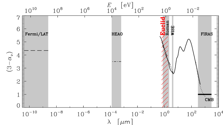
Figure 24: The Compton-Getting dipole amplification, $(3-\alpha_{\nu})$ shown for various wavelength data marked on the horizontal axis. For high-energy data the upper horizontal axis marks the corresponding energy, $E$. From left to right: dashes mark the amplification for the Fermi-LAT data, dashed-dotted line for the HEAO X-ray data, solid line for the mid- and near-IR data, dashed-triple-dotted line for the near-IR IGL at $m_{0}\geq 18$ and the dotted line shows the amplification the far-IR CIB determined from FIRAS. See text for details. The range of wavelengths covered by each line is marked with shadow rectangles. Euclid is marked in red being the subject here.