¹¹affiliationtext: Complex Human Behavior Lab, Fondazione Bruno Kessler, Trento, Italy²²affiliationtext: MLG, Université Libre de Bruxelles, Brussels, Belgium

Drift Diffusion Model to understand (mis)information sharing dynamic in complex networks

Lucila G. Alvarez-Zuzek lalvarezzuzek@fbk.eu Jelena Grujić Riccardo Gallotti rgallotti@fbk.eu

Abstract

Sharing misinformation threatens societies as misleading news shapes the risk perception of individuals. We witnessed this during the COVID-19 pandemic, where misinformation undermined the effectiveness of stay-at-home orders, posing an additional obstacle in the fight against the virus. In this research, we study misinformation spreading, reanalyzing behavioral data on online sharing, and analyzing decision-making mechanisms using the Drift Diffusion Model (DDM). We find that subjects display an increased instinctive inclination towards sharing misleading news, but rational thinking significantly curbs this reaction, especially for more cautious and older individuals. Using an agent-based model, we expand this individual knowledge to a social network where individuals are exposed to misinformation through friends and share (or not) content with probabilities driven by DDM. The natural shape of the Twitter network provides a fertile ground for any news to rapidly become viral, yet we found that limiting users’ followers proves to be an appropriate and feasible containment strategy.

Introduction

As individuals, we understand the world by constantly acquiring new information. The advent of the Internet has released numerous opportunities for information to spread faster and more expansive, reaching more people than ever before. However, the amount of information at our fingertips seems overwhelming, exposing us to a considerable amount of untrustworthy information [1]. This may lead to dangerous behaviors that for instance, may burden the acceptance of vaccines [2], produce a negative effect on the public image of a political candidate through false narratives [3, 4], etc. The term misinformation refers to information that is false but not created with the intention of causing harm [5, 6, 7], for instance, individuals sharing online pieces of information without knowing that it is false and intending to be helpful. False information may have the capability of changing our perception of reality [8] and its diffusion in a society may have serious consequences, such as compromising our ability to address hence fight the climate crisis [9], enhance public health systems [10, 11, 12], or maintain a stable democracy [13, 4]. But why do people share false or unreliable information on social media? The scientific community has been studying this topic for decades. In [14], the authors found that analytic thinking plays an important role when it comes to false political information. People tend to share it because they fail to think. Moreover, they suggested that susceptibility to fake news is driven more by lazy thinking rather than by partisan bias. On the contrary, in [15] Ceylan, $et.al.$ found that the structure of online sharing in the platform is more important than critical reasoning or partisan bias. That is to say, users tend to form habits of sharing misinformation and react automatically to familiar platform cues (in their case of study Facebook). Habitual sharers do not take into consideration the informational consequences of what they share. Altogether, these pieces of research may suggest that the decision-making process of sharing false information is made rapidly and at a low cognitive level.

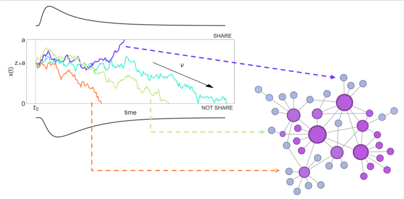
Daily life activities involve the process of decision-making, whether to cross or not a street, which candidate to vote for, or when to take holidays. Some decisions are more important and require a deeper analysis. While others are made rapidly (almost instantaneously) and with less cognitive effort. Mathematically, cognitive processes that involve simple and rapid two-choice decisions can be seen as the noisy accumulation of evidence from a stimulus and can appropriately be described by Drift Diffusion Models (DDM) [16]. These sequential sampling models have been extensively studied for decades, building a bridge between neuroscience and human behavior, taking advantage of collected data [17]. Starting with the model proposed and developed by Ratcliff in [18], the DDM assumes a one-dimensional random walk representing the accumulation in our brain of noisy evidence in favor of one of the two alternative options. More in detail (see Fig.1), the process is represented as the temporal evolution of a random variable $x(t)$ from a point $z$ named the bias. At each time step, as information is randomly collected in favor of one of the two choices, this accumulation is represented as increases or decreases in $x(t)$ up until a decision is made when one of the boundaries is reached $x=a$ or $x=0$ (being $a$ the boundary separation). The information accumulation rate is called the drift rate $\nu$ (see Methods for a more detailed mathematical description of the model). From a neuroscience perspective, these free parameters of the mathematical model have the following interpretation: (i) The bias ( $z$ ): is related to the prior inclination (the pre-existing ideas) the individual has about the options, (ii) The threshold or length of the barrier ( $a$ ): psychologically quantifies cautiousness in response, (iii) The drift rate ( $\nu$ ): the value of this quantity is related to the quality and velocity of the information extracted from the stimulus, also related to the task complexity. For tasks “easy” to understand, the drift rate has a high absolute value, and responses are fast and accurate on average. Conversely, when subjects find the tasks “difficult”, the drift rate values are closer to zero, and responses are slower and less accurate on average. The accuracy of this model is measured with the response times (RTs) and response times distributions (PDF). By evaluating the predictions of the model with the shape of the response time data, we can obtain the free parameters and test the performance of the model. Previous studies have shown that decisions with smaller response times are more intuitive and less accurate, while longer decisions are more deliberate [19]; it is important to understand whether a person responds as quickly as possible or as accurately as possible. Hence, researchers generally focused on how response time probabilities change across experiment conditions (variations may appear among ages, genders, political orientations, etc.). Many variations to this model have been explored, such as adding non-decision time [20], across-trials variability of the rate of accumulation of information [21] and the starting point [19], speed-accuracy optimality [22, 23] and more [24]. Additionally, more sophisticated models have been developed, mainly physiologically motivated by cases that involve more than two-option decisions [25]. For instance, the race model uses separate accumulators for each of the options, integrating evidence independently.

The universality of the Drift Diffusion Model allowed scientists to use it in a wide spectrum of different topics. In game theory, previous research used the model to describe and explore human cooperation-defection [26]. Finding that, in this context, individuals initially tend to cooperate, but rational deliberation quickly becomes dominant. And depending on the interaction with the environment a positive or negative experience will be translated into a cooperative or defective answer. DDM models have also been used to describe human behavior in the context of altruism [27], food choices [28], moral judgments [29], and more. In the context of online sharing misinformation, Lin. $et.al$ [30] investigate accuracy and deliberation when sharing misinformation. They found that accuracy prompts increased sharing discernment by shifting peoples’ attention to accuracy while deciding what to share rather than increasing the amount of deliberation; this is interesting because they show that people can think better even without thinking more. However, not much is known about this topic, and there is still much more to understand. For instance, can we take advantage of drift-diffusion model to describe the decision-making process of sharing online misinformation? Is it a suitable model for this kind of cognitive response? How well is the model’s performance, and how does it vary across experimental conditions, such as age and other factors? In this research, our first aim is to explore and understand these addressed issues.

At the moment, diffusion models link cognitive and behavioral decision-making processes at an individual level, providing a solid theoretical framework. But we know that social interactions play a fundamental role in human behavior, and interesting and unexpected outcomes can emerge from collective phenomena. Widespread misinformation can lead to macroscopic clusters of people sharing misperceptions and biased collective opinions [13], for instance, leading pools of vaccine-hesitant individuals susceptible to a new epidemic outbreak [31, 32]. Further, it is well known that when certain features are present in the social patterns —namely homophily [33], polarization [34], echo chambers characteristics [35, 36, 37]— they have a strong impact providing a fertile ground for the spread of misinformation [38]. Thence, our next step here, is to expand these micro-level concepts to a macro-level. How can we link these neurocognitive mechanisms of decision-making taking place inside the brain of each individual (micro-level) to misleading content spreading and going viral on an online platform (macro-level), such as Twitter?

The present research explores the decision-making process of sharing misleading information online with two-fold goals. As a first step, we took advantage of the universality of the Drift Diffusion Model to describe and analyze data collected by G. Pennycook & D. G. Rand in [14]. In this study, misleading and reliable content was presented to participants to then ask how prone they were to share it with response option yes, maybe or not (three-option process). To be able to apply DDM, we reduce the dimension of the problem by combining the positive options and analyzing the performance of the model. Data is disaggregated by content, content veracity —misleading and reliable— and age, and variation in the free parameters of the model are present across the different experiment conditions. As a second step, we aim to expand this individual-level mechanism to a population level; a broader perspective in which we explore how the social contact patterns impact the outcomes of the collective behavior. We consider a social network with similar structure characteristics as the Twitter network described in [39]. Then, to mimic the propagation of information, we propose to use an agent-based model in which individuals are divided into two compartments: Sharers ( $S$ ) or Non-Sharers ( $NS$ ). Every time an $S$ individual shares content will activate the decision-making process in their $NS$ neighbors. That is to say, a single DDM process runs, giving an answer (share or not) to the stimulus. Finally, we use the previous mathematical framework in [40] to build a bridge between the micro and macro levels and obtain the critical conditions the free parameters should satisfy in order for (mis)information to become viral; this leads us to propose as an intervention strategy to limit the number of accounts that can follow a user.

Refer to caption — Figure 1: Information spreading in a society considering the neurocognitive mechanisms driving each individual response. On the right side is the social network on top of which the spreading process occurs, $i.e.$ , information diffuses in the social media platform where users interact. Every time an $S$ individual shares content (violet), its $NS$ neighbors will see it, and a single decision-making process is activated (for each of them) to decide whether to share or not the content (on the left side).

Results

What motivates individuals to share or not share content? What are the neurocognitive mechanisms driving the decision-making process? Do these mechanisms vary with the nature of the content? Does information spread vary with individuals’ characteristics? In this Section, we explore if and how the Drift Diffusion Model can model the decision-making dynamic of sharing misleading and reliable content. We use the open access dataset presented in [14], where authors carried out a large-scale experiment in which participants discerned the veracity of news headlines and expressed how prone they were to share them. Data was collected from a total of $N=2644$ participants with an age range from $16$ to $88$ . Each experiment consisted of presenting to participants $12$ reliable and $12$ misleading content. All misleading news headlines were originally taken from Snopes.com; while reliable headlines were selected from mainstream news sources (e.g., NPR, The Washington Post). All content was contemporary (see Methods for more details). Additionally, we explore how contact patterns affect the possibility of viral content and the role played by the free parameters of the DDM.

Drift Diffusion model is capable of capturing decision-making process of sharing information

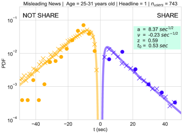
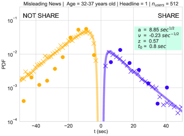
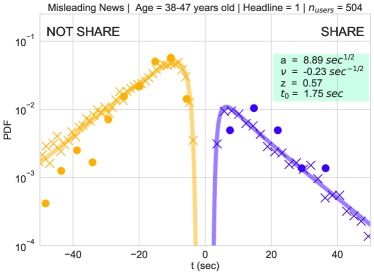
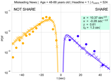
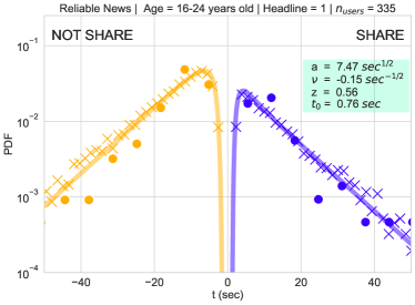
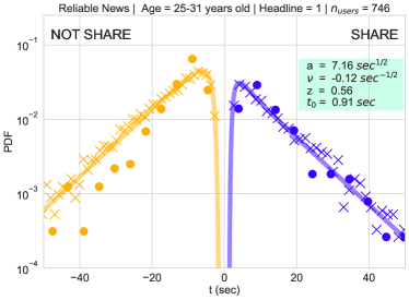
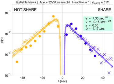
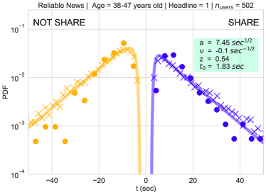
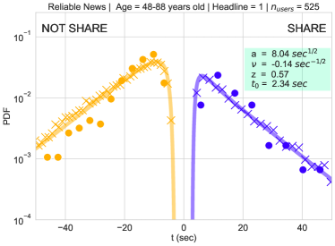
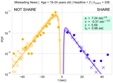
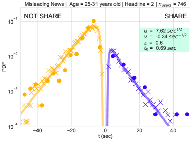
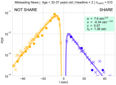
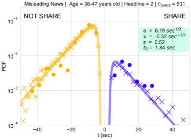
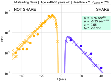
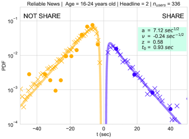
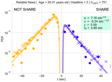
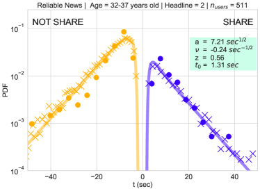
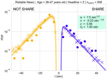
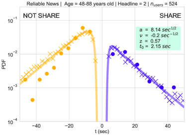
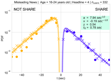
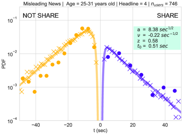
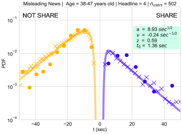
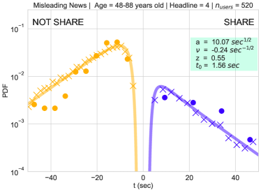
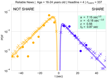
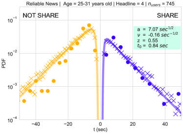
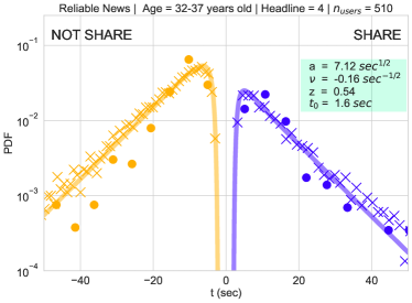
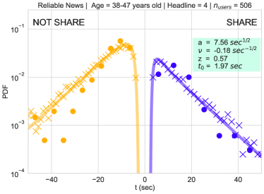
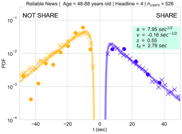
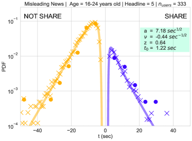
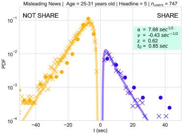
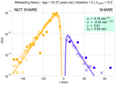
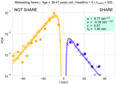
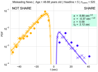
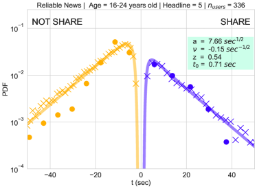
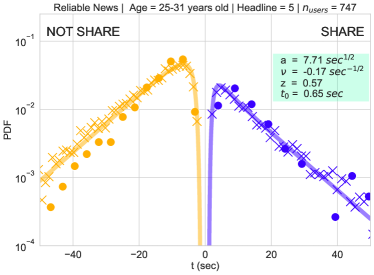
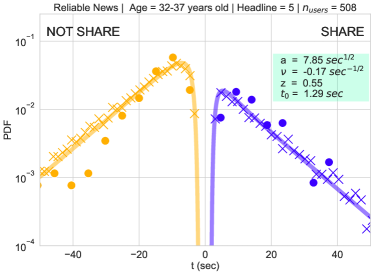
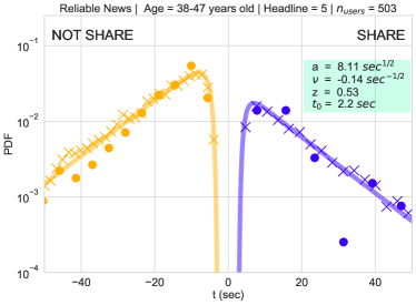
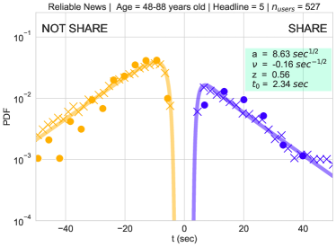
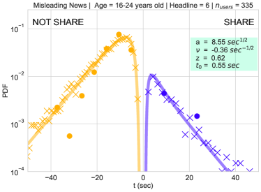
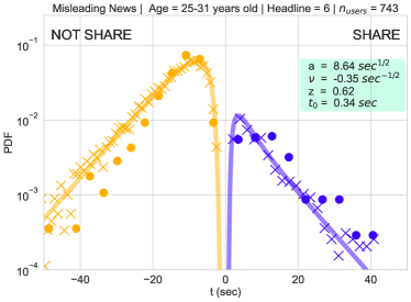
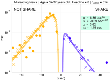
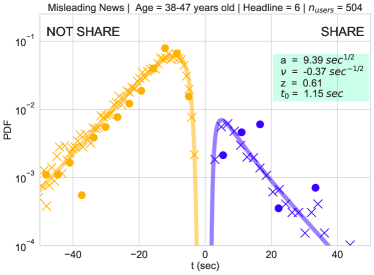
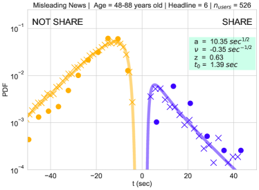
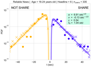
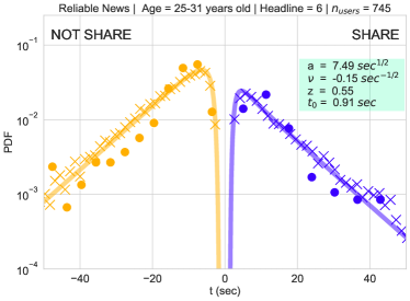
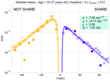
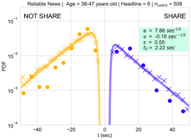
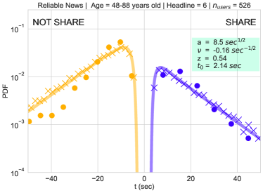
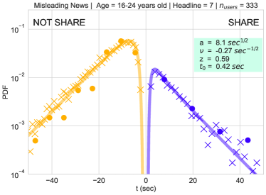
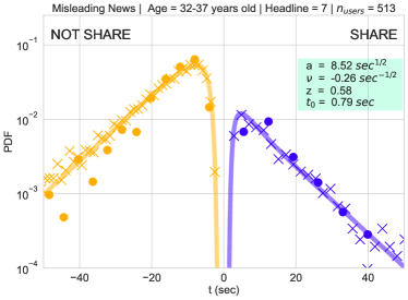
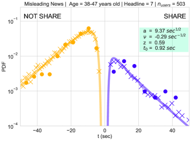
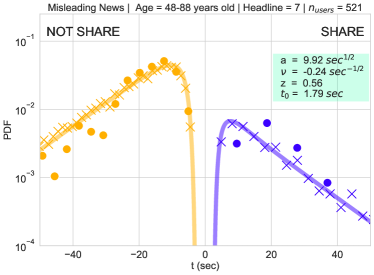
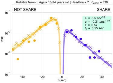
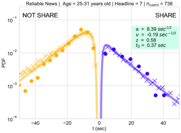
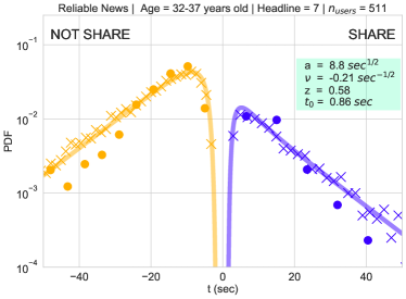
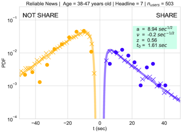
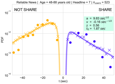
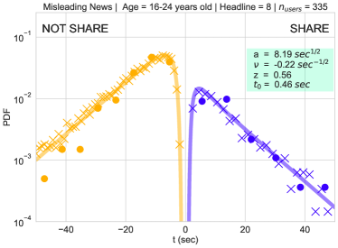
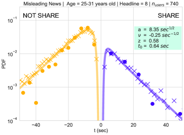
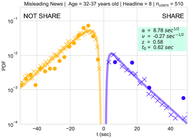
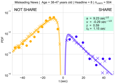
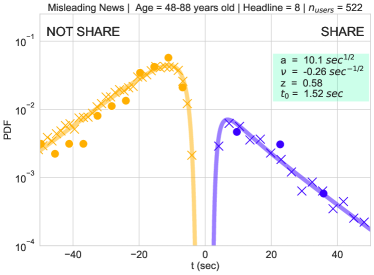
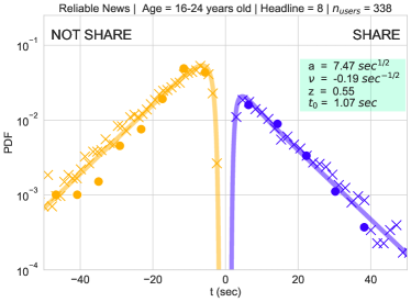
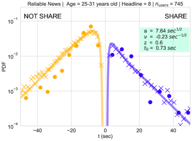
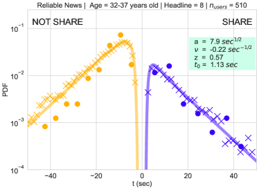
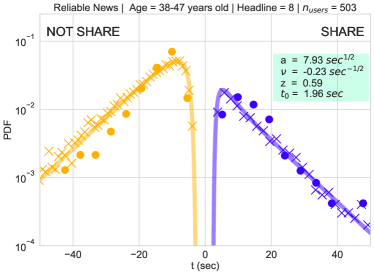
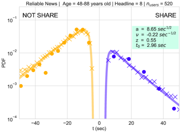
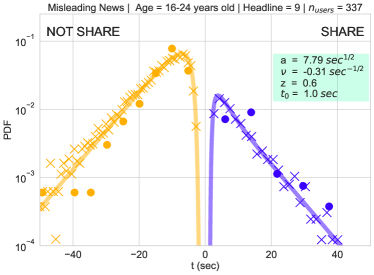
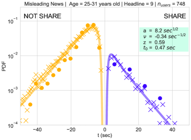
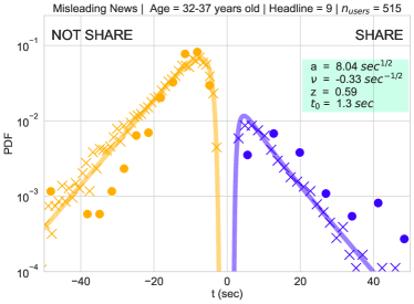
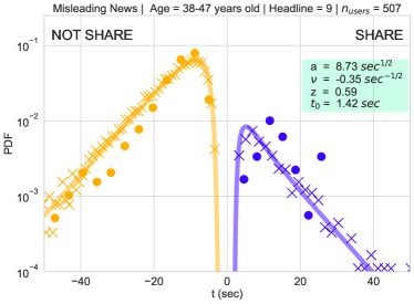
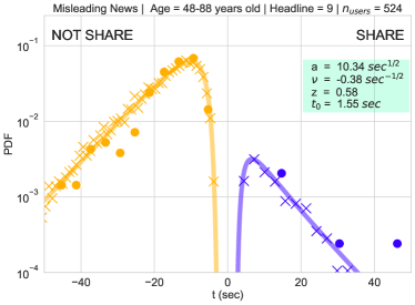
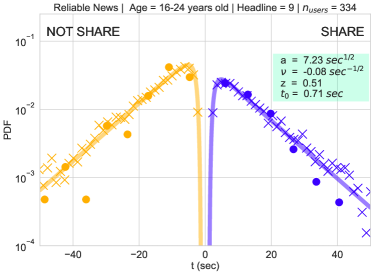
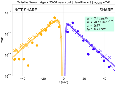
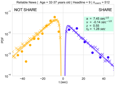
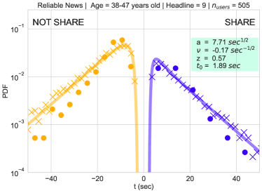
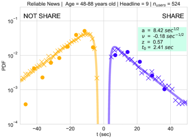
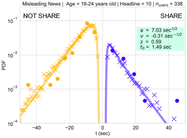
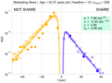
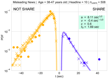
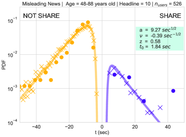
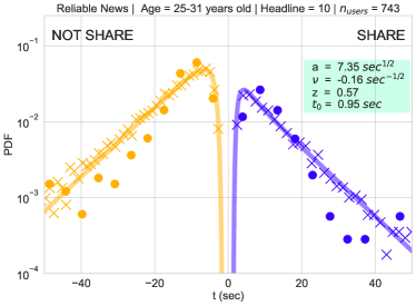
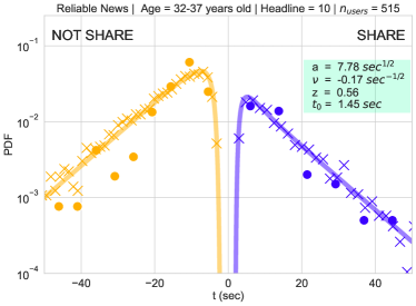
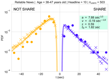
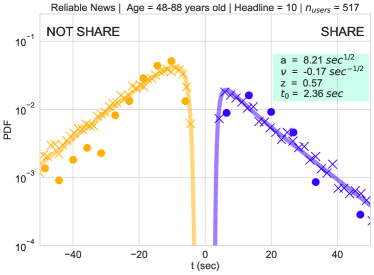
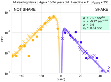
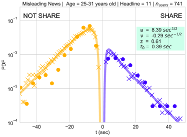
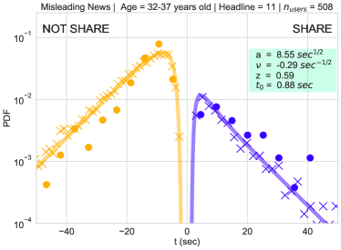
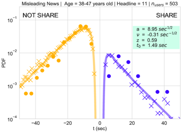
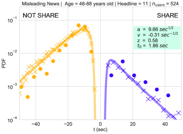
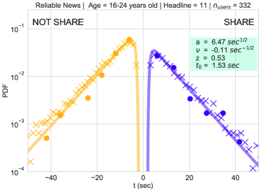
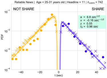
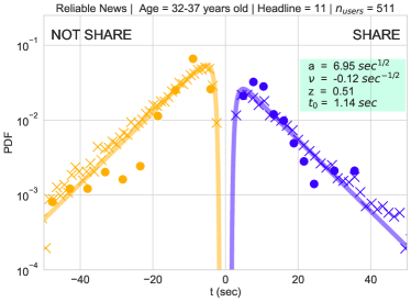
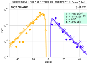
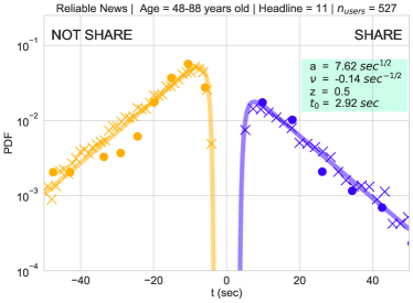
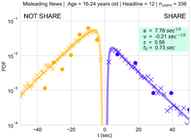
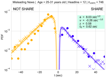
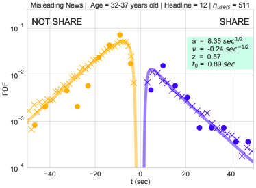
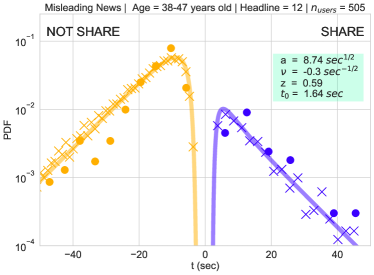
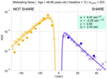
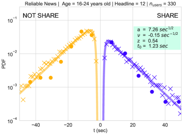
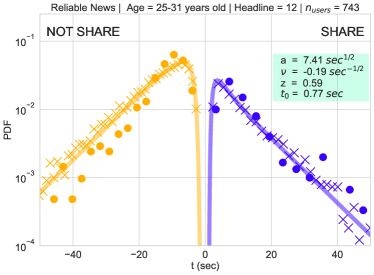
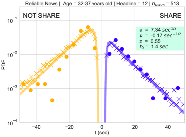
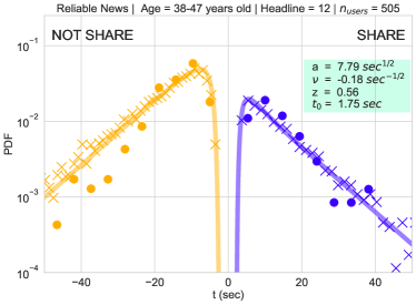
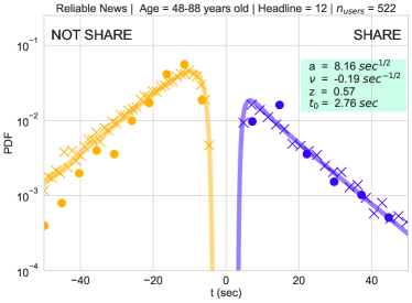
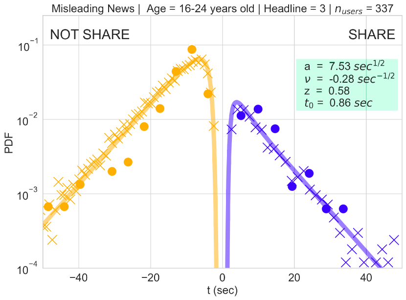
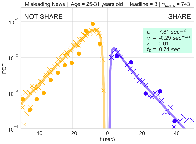
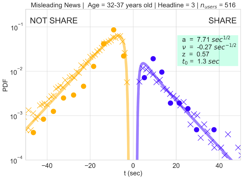
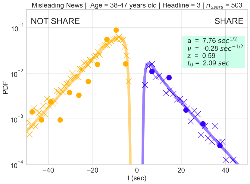
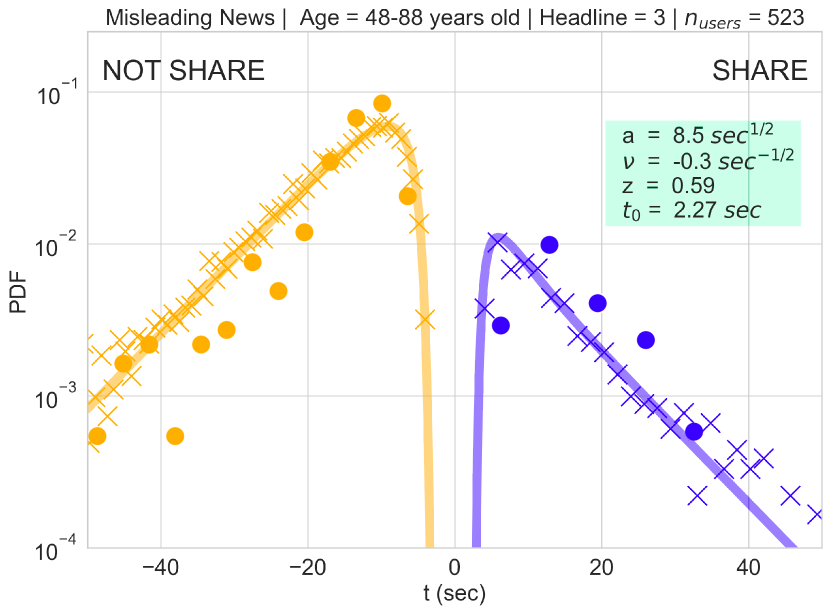
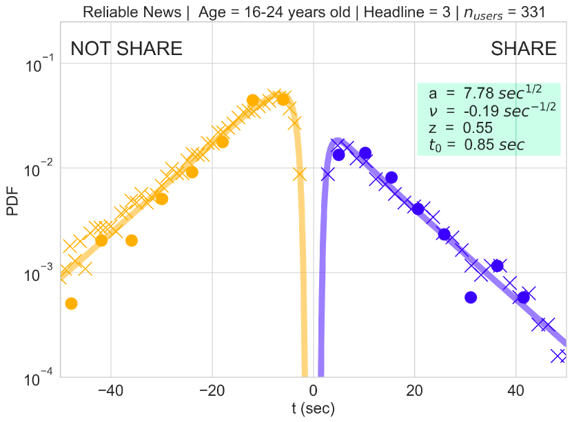
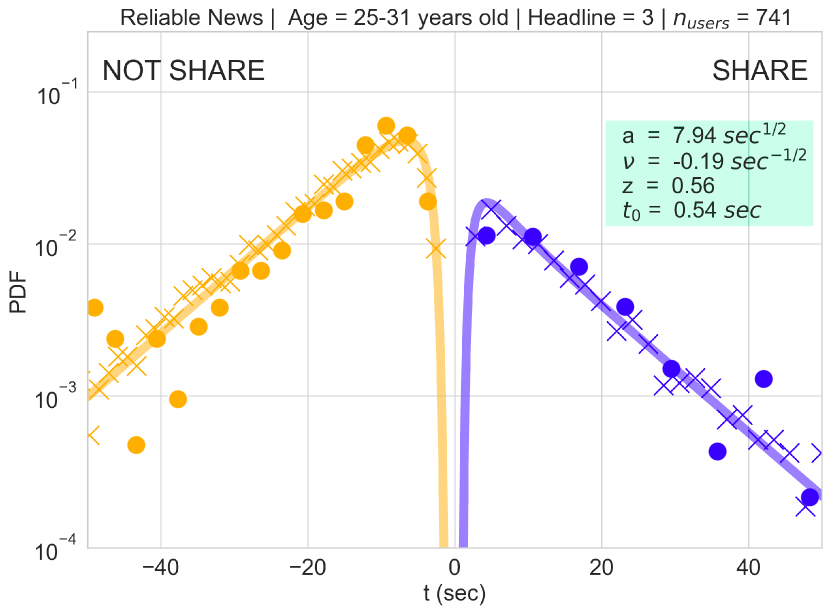
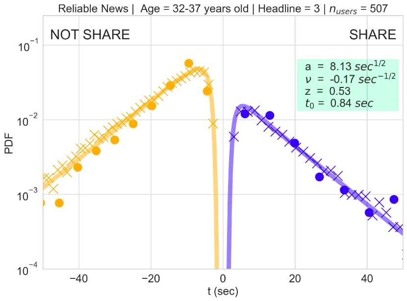
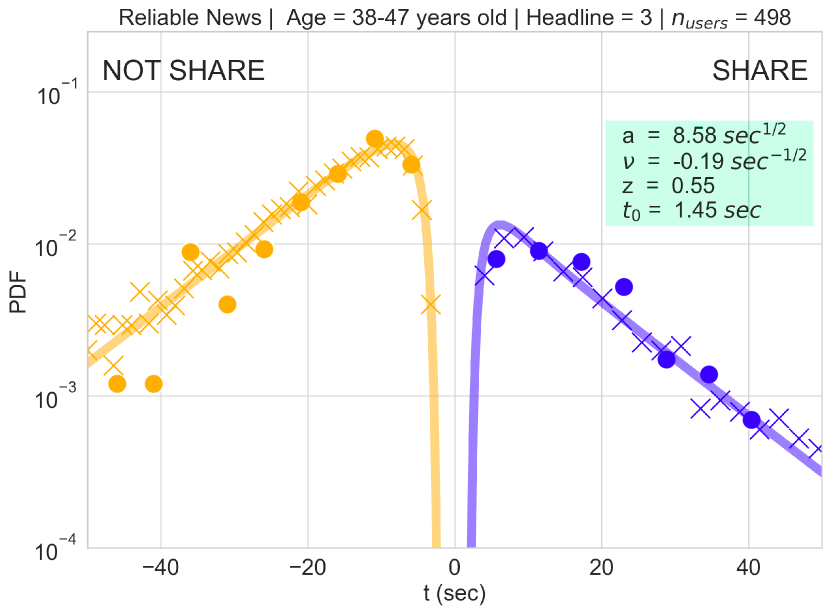
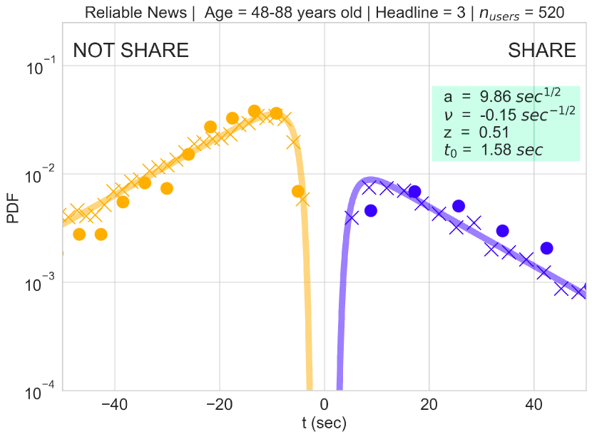
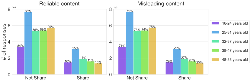
A decision-making process with two options as possible answers can be well-modeled by the Drift Diffusion Model [24] (see Methods). However, this is not the case for three or more responses. Typically, this kind of scenario can not be well described with a one-dimensional dynamic, and there are more suitable models, such as the race model [25], in which accumulators for each alternative integrate evidence independently. To be able to use DDM to describe the dynamic, we reduce our problem to two dimensions. We assume that “no” responses are the only representative of not sharing (individuals here are determined not to share the content), and the rest of the answers, “yes” and “maybe”, are in an undecided grey area, mostly prone to share the content. As described in the Methods Section, we applied the Hierarchical Drift Diffusion Model [41] to obtain the set of parameters that better represent the data. Following, we display the probability density functions (PDF) of the response times (RTs) for the case of misleading in Fig. 2 and reliable content in Fig. 3. A good agreement is obtained between empirical data (dots) and theoretical results (solid lines), which are derived by Eq.(1) and using the set of parameters in the legend (legend box, and see methods for further details on the dimension of the free parameters). We disaggregated our data by age range: $16-24$ , $25-31$ , $38-47$ , and $48-88$ years old, and headlines: $12$ misleading and $12$ reliable; and we consider answers with $RTs<100$ seconds (see the sensitivity analysis in Supplementary Fig. 1. Besides, we classify the RTs according to individuals’ responses, with a positive orientation for the case of sharing (orange left side) and a negative orientation for the case of not sharing (violet left side). For simplicity, we only display headline number $3$ , but all headlines can be found in the Supplementary Information. In addition, Fig.4 displays the bar charts of the number of responses when sharing and not sharing for reliable and misleading content. Note that these results have already been analyzed in [14]. From Figs. 2-4, we can see that the decision not to share is more trendy than the decision to share, and this is consistent among all ages and independent of the content. Besides, as already observed in [14], deciding not to share in general takes more time, $i.e.$ , higher RTs have a higher probability for the not sharing scenario. And in a misleading scenario (Fig. 2), this difference is more noticeable. An explanation for this could be that individuals prone to sharing may do it as a reflection or a habit, as suggested in [15]; they do not take much time to think about the decision and do it automatically. While the decision not to share requires more analysis, longer times have more probability, meaning that individuals need to gather more evidence (probably) to discern the content’s veracity and if they are prone to share it. Finally, in a reliable scenario (Fig. 3), we can see that longer RTs now have a higher probability in both cases.

Neurocognitive mechanisms differ among ages and veracity of the content

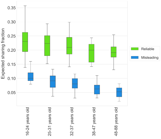
In this Section, we estimate the free parameters of the DDM. The fit of the parameters has been performed using the HDDM Python-based toolbox [41], which uses the Hierarchical Bayesian Estimation to simultaneously fit the distribution of response times for both options -share and not share-. In Fig. 5, we show the results for the cases of (a) misleading news headlines and (b) reliable news headlines, where plots correspond to a different parameter, and each box plot shows the distribution of each range averaging over the $12$ headlines. Notice that even though the nature of both headlines differs, we can see similar trends in both cases -misleading and reliable-.

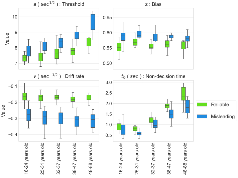
Threshold ( $a$ ): This parameter is also known as the “criterion” or the “decision boundary” and is related to the amount of evidence required to trigger a decision response. Speed-accuracy trade-off is modeled by this parameter. If accuracy is emphasized, boundary values tend to be higher and far from the starting point; in this way response times are slow, and accuracy is high. Conversely, when speed is emphasized, boundary values tend to be lower and closer to the starting point; in this way, individuals respond faster, leading to lowered accuracy due to the fact that processes that would have reached the correct boundary now are more likely to reach the wrong one by mistake [19]. From Fig. 5, we see a tendency in age to become more cautious when sharing any information independently of their nature. However, in the case of misleading content, the increase in cautiousness over age is considerably larger. From Fig. 4, we can see that both -younger and older people- are more prone not to share this type of content. This may imply that the parameter is greater for older generations because they take more time to discern the content’s veracity.

Bias towards sharing ( $z$ ): The bias parameter indicates the starting point for the decision-making process, and it is related to the initial inclinations of the individuals; that is to say, the pre-existing ideas individuals have about the topic. In our case study, if initially subjects are more toward sharing, the starting point will be closer to the corresponding boundary $a=1$ . Otherwise, it will be closer to $0$ (not sharing). From Fig. 5, we can see that, in principle, individuals tend to be slightly biased toward sharing both types of content since $z\geq 0.55$ and have, therefore, an instinctive inclination to share content. The bias for reliable headlines, in particular, remains almost constant across ages and appears systematically larger for misleading headlines. This suggests that subjects may have an amplified intuitive inclination to share misleading news.

Drift rate ( $\nu$ ): This parameter is related to the information acquisition, and it measures the subjects’ ability to gather evidence of the stimulus related to the task complexity. The module $|\nu|$ specifically indicates the rate at which individuals process the information given by the content to understand if they are willing to share it or not. From Fig. 5, we can see that the values tend to be closer to zero, implying that the stimuli are “difficult” to understand and the information gathering is slow, particularly regarding reliable information. For misleading content, the task seems easier. On the other hand, the negative sign of the drift suggests individuals’s rational thinking leads more toward not sharing information in general, independently of the veracity of the content and ages. Lastly, we can see that there is not much difference among ages; for younger people, it is slightly less challenging to understand the content, but the difference is not significant enough to draw strong conclusions.

Non-decision time ( $t_{0}$ ): This parameter corresponds to the time before the decision process begins, is the component of RT that is not due to evidence accumulation, and is more related to the physiological components of the experiment. For instance, it could be related to the time individuals take to prepare themselves to start reading the headline (before they realize that the new round started) or the time used to press the bottom of the mouse. As expected, we can see almost no difference between the two types of content. Yet, there is a noticeable difference among ages: young people tend to be faster, while older people tend to be a bit slower and take more time to start with the task.

In an unbiased scenario ( $z=0.5$ ), when $\nu$ reaches high values, faster and more precise decisions are taken. In addition, high values of the $a$ reduce the role of noise, producing slower yet more accurate responses. Consequently, we can explore the speed/accuracy trade-off in our cases of study in a hypothetical absence of bias. In this context, we conclude that older generations tend to be better thinkers, especially in the case of misleading content. Their trade-off is superior to younger generations due to higher values of $a$ and $\nu$ ; they are faster towards not sharing and more accurate. Besides, we can also see in Supplementary Fig. 2 that the expected fraction of individuals towards sharing is higher for younger people who appear to be more reckless or lazy thinkers. This raised point offers an alternative but aligned interpretation of the results obtained by [14] on this same dataset.

Contact patterns matters on going viral

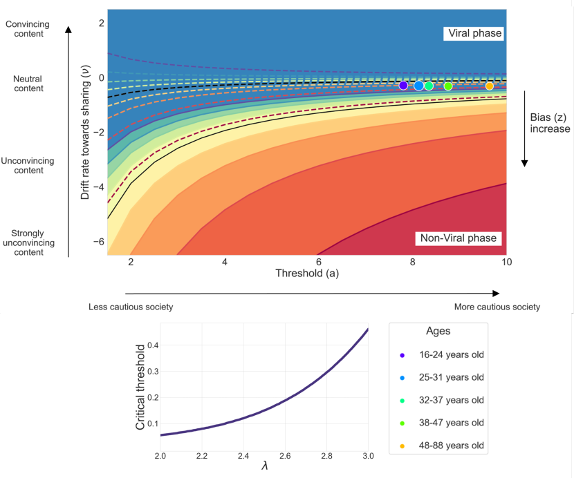
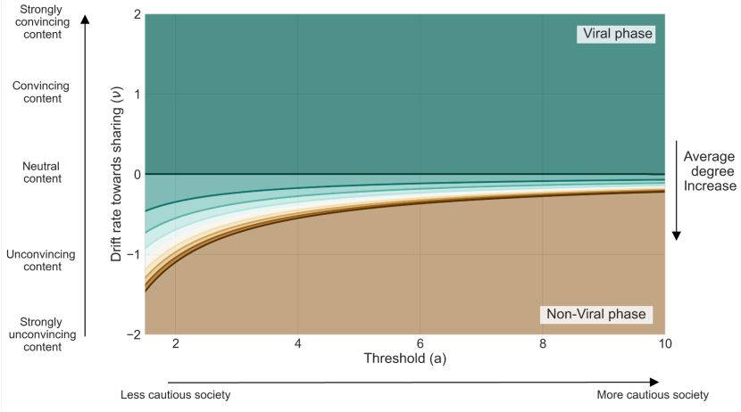
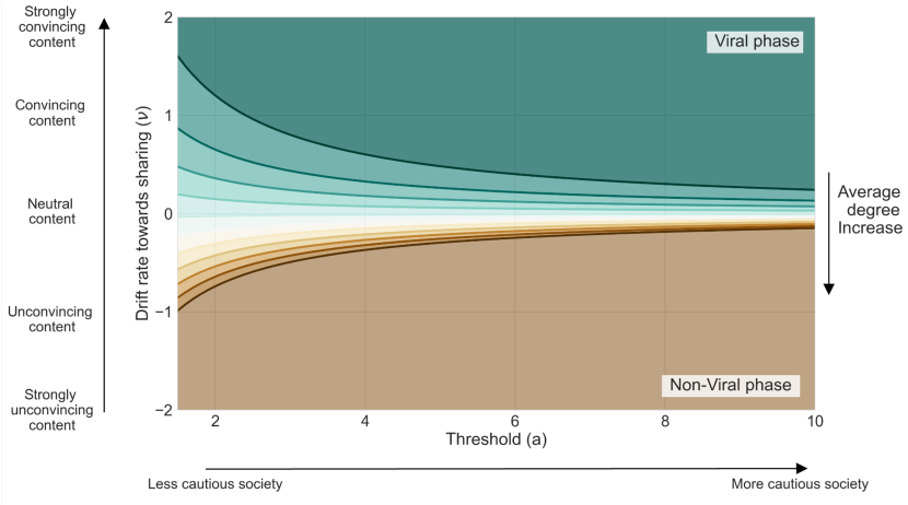
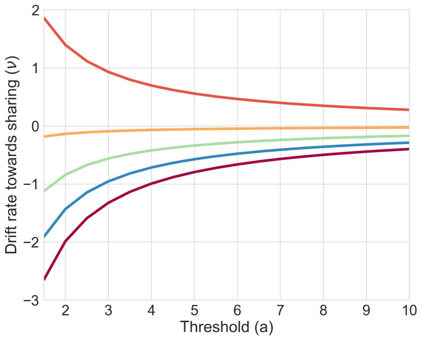
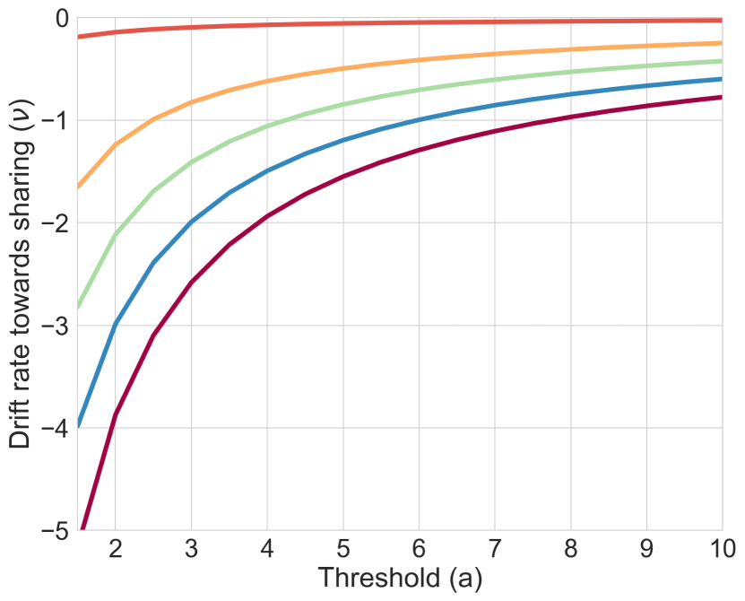
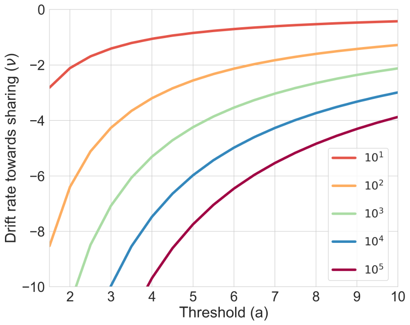
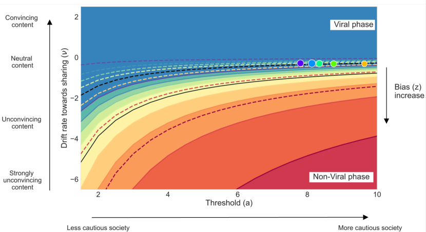
How should the neurocognitive characteristics of society be to provide fertile ground for content to become viral? Do the storytelling and the nature of the content play an important role? As a final step to answer these questions in this Section, we build a bridge between the individual-level concepts presented before and the collective behavior of the population (see Methods for details). We assume all individuals of the society to be identical and following a DDM. The condition for virality in this society is given by the expression given of Eq. (3) for critical threshold values of the free parameters of DDM: threshold $a_{c}$ , drift $\nu_{c}$ , and bias $z_{c}$ . Notice that the non-decision times do not influence the mechanics behind the binary choice. In Fig. 6, we display the transition diagram for the critical values of the free parameters of the DDM that divides two phases: the Viral content and the Non-Viral content phase. Meaning that all the possible combinations of parameters above the curves correspond to those scenarios in which the content becomes viral in that society. Conversely, in all cases below the curves, the content fades off. For the social contact network, we mainly focused our study on a network with similar characteristics as Twitter [39], a Power Law with $P(k)\sim k^{-\gamma}\;exp(-k/\kappa)$ with $\gamma=2.2$ and $\kappa\approx 10^{5}$ (solid lines), and we also explore an extreme intervention scenario with $\kappa=20$ proposed by [40] (dashed lines). See Supplementary Fig. 4 for more details on the cutoff dependency. Notice that here we are not considering the competition between news; in our case study, there is only one type of news spreading, and its viralization only depends on the characteristics of the population, the network structure, and the nature of the content.

In the x-axis of Fig. 6, we can see a clear division of societies in two: a less cautious one with low values of $a$ hence response times are shorter on average, and individuals tend to make faster decisions being more reckless (left); a cautious one with high values of $a$ , where response times are slow, subjects take time to gather evidence and thinking more before making a decision (right). On the other hand, the y-axis corresponds to the characteristics of the content, the storytelling.

For high positive values of the drift (green-blue area), the gathering of information is fast due to the stimuli being easy for the individuals; this means that the content is clear and strongly convincing; thus, subjects are more prone towards sharing independently on the veracity of the headline. Instead, for intermediate values when $\nu\approx 0$ , the stimuli are difficult. Individuals find themselves undecided whether to share or not the content, and this is due to its neutral nature (yellow area). Lastly, for high negative values of the drift (orange-red area), the gathering of information is fast, and the stimuli are easy. However, this is due to the content being strongly unconvincing; thus, subjects are more prone to not sharing. Jointly, lines are incorporated by varying the bias $z$ , from $0.1$ (top), where individuals tend to be a prior more prone not to share content, increasing to $0.9$ (bottom) with $\Delta z=0.1$ , where individuals tend to be a prior highly towards sharing information.

In general, in less cautious societies, we can see that the bias plays a crucial role in the viralization of the content. If individuals are a priori towards not sharing content, the story should be compelling in order to become viral. On the contrary, for a less biased society, even challenging to understand may become viral. In this scenario, individuals tend to be reckless and may give a response more out of habit than reasoning. A different outcome emerges for more cautious societies; individuals need to gather more information before making a decision, and the role of the bias slowly vanishes. Here, the nature of the content becomes relevant if its convincing will become viral, and even neutral content may be enough.

Additionally, we incorporate the set of values of the parameters obtained from the empirical data (colored dots). Each dot corresponds to a different age range, and the size corresponds to the value of $z$ , being close to $\approx 0.55$ for all the cases. This bias value corresponds to a neutral content situation (yellowish area) from the theory. As we can see in Fig. 5, for the case of misleading content $\nu_{empirical}\approx 0.3$ , for all age ranges. The values of $a$ , $\nu$ , and $z$ extracted from the experiment are, therefore, below the critical threshold (yellowish area) needed to become viral. Although, in principle, the population does not provide an appropriate ground to viralize the content, it is lightly close, $i.e.$ small changes in the parameter(s) are necessary to go viral.

Modifying the structure of a network could be challenging, particularly in topologies as large and complex as Twitter. Yet, intervention strategies, such as limiting the number of accounts that can follow an individual seem to be a realistic scenario to implement. Thus, we explore how reducing the maximum degree of users impacts the viralization of news. To do that, we describe in Fig. 6 with dash lines the same network structure as before $P(k)\sim k^{-\gamma}\;exp(-k/\kappa)$ with $\gamma=2.2$ , with an extremely reduced cutoff $\kappa=20$ (inspired by [40]). As we can see, the reliability of the content becomes more relevant, bringing up a significant reduction in the viral phase areas included in the diagram. For the unbiased scenario (black dashed lines) unreliable content cannot become viral. The network structure still favors viralization, yet not enough for any type of content to spread. Interestingly, for the cases of populations biased toward not sharing ( $z<0.5$ ), only convincing content will become viral. And, for populations biased toward sharing, no major changes appear. Furthermore, we also explore a more realistic scenario with a cutoff $\kappa=150$ , corresponding to Dunbar’s number. In [42], authors analyzed a dataset of Twitter conversations and tested the cognitive limit on the number of stable social relationships (known as Dunbar’s number), finding that users can entertain a maximum of 100–200 stable relationships. In Supplementary Fig. 5, we illustrate this intermediate scenario where the impact of the cutoff is comparable with the cutoff $\kappa=20$ discussed so far. Therefore, a potential containment strategy would be limiting users to reach a number of connections less than the natural Dunbar’s number and, in this way, reduce the leverage provided by social media that empowers few ”influencers” to have almost unlimited reachability. Our real-life scenario shows that this strategy would be effective for both $\kappa=20$ (Fig. 6) and $\kappa=150$ (Supplementary Fig. 5). From Fig. 5, we know that $0.55<z<0.6$ , and this is associated with the yellow area in the diagram. In the conditions we are simulating here, where one piece of news is monopolizing the media, we can see that normally it will become viral, given that it is above the yellow area. However, with the extreme intervention scenario, it is possible to modify the topology enough so that it will not push the condition below the dashed yellow line. Remarkably, in the case, $\kappa=150$ (Dunbar’s number, see Supplementary Fig. 5), seems to lie closely to the critical point where news might become viral (or not) randomly.

Finally, in the bottom part of Fig. 6, we added the dependency of the critical values as a function of the network structure for the standard SIR (left part of Eq.(3)). In the case we are focused on with $\lambda=2.2$ , the critical threshold is $\approx 0.1$ . And, as we can see, as $\lambda$ increases, the structure becomes more homogeneous, and the critical value increases. This means it is harder for the content to diffuse through the entire population. The opposite happens when the structure becomes more heterogeneous; once the content reaches a highly connected subject, it spreads rapidly through the whole population, and the critical threshold is lower.

Additionally, in the Supplementary Information, we explore the dependence of the phase diagram on the network structure. As we can see in Supplementary Fig. 3, a great impact of heterogeneity is reflected in the critical values of the free parameter. These results highlight the importance of the network structure in these processes with a diffusive nature.

Discussion

Not all information is trustworthy and safe to share. Occasionally, false information could be malicious and have the capability to change our perception of reality, creating confusion and compromising our welfare. In this information landscape, we wonder: Why does information successfully spread through an entire society? Which characteristics should the populations have to provide a fertile ground for this phenomenon to emerge? At what level do the neurocognitive mechanisms of each individual affect the spreading, and conversely, at what level do the social contact patterns impact?

In this research, we study the decision-making process of sharing information —misleading and reliable— online. We take advantage of the universality of the Drift Diffusion Model to mathematically describe the response of individuals to share potentially misinformative content. By obtaining a solid accuracy (in the response times) between our model and the data, we analyzed the neurocognitive mechanisms of the process by tracking the free parameters of the DDM. The model is well-known for describing decision-making processes with two-option responses, different from our three-option response problem. Yet, here, we can reduce our problem and find a perfect accuracy between the DDM and the data. Then, we built a bridge between this individual behavior (micro-level) and the collective behavior (macro-level), using a social network approach to describe the social contact patterns. Finally, we develop a mathematical approach that allows us to obtain the phase diagram of the viralization of content, where all the micro and macro information is merged. The diagram is a joint junction of the neurocognitive characteristics of the individuals, the features of the content, and the network structure, from where we may be able to predict if the content will go viral in a particular society. This approach also allowed us to study, as an intervention strategy, the impact of limiting the maximum number of followers a user can have.

Regarding the neurocognitive parameters of the model, there is a difference in all our results, which is related to the content’s veracity. Firstly, individuals tend to be more cautious and hence take more time to decide whether to share misleading content. And this cautiousness is further accentuated with age. Secondly, individuals of all ages a priori tend to be slightly prone to instinctively share news headlines and more likely to if the content is misleading. This difference may be explained by the fact that misleading content creators are actively attempting to leverage emotions to generate engagement in their readers [43]. Thirdly, in general, when individuals gather information concerning a news headline, the stimuli they receive tend to be directional in favor of not sharing content. And in the case of misleading content, the trend runs deeper.

By differentiating societies in their level of cautiousness when making a decision, our results suggest different and interesting scenarios. For less cautious societies, the bias plays a more important role in the spread of information. In this context, individuals respond faster, being more reckless and directing their answers towards their pre-existing concepts. Conversely, in more cautious societies, the effect of the bias fades off (specially for low values), bringing up more importance to the nature of the content and how convincing is the news headline. This behavior runs much deeper when there is a limit on the number of users an individual can be connected to. In the context of intervention strategies, such as in predicting the effects of pre-bunking [44] or automated debunking interventions [45], our results suggest that it is of utmost importance to detect the features of the targeting population. Both the average age of individuals and the structural characteristics of the social networks play crucial roles in determining the spreading dynamics. Younger and less cautious societies tend to be a more fertile ground for misinformation spreading. At the same time, even strongly unconvincing content may become viral if the network structures, where a smaller number of influencers dominate the spreading process, provide that individuals are biased toward sharing content. Unfortunately, our result suggests that the natural shape of the Twitter network provides fertile ground for rapid viralization. Modifying the network strategy with, for instance, re-wiring/deleting connections could be challenging. For this reason, we propose to impose a limit on the number of followers an individual can have. We find that an extremely reduced maximum in-degree should be imposed in order to enhance the importance of the characteristics of the population (measured by the bias and the barrier) and the nature of the content (measured by the drift). Notice that, in our case study, we are considering experimental conditions representing a monopolization of the media, where there is only one piece of information propagating in a society.

Our work has some limitations. On one hand, our aggregation in the data considers that all individuals are a replica of the same “average subject” of a specific age range, independently of gender, or political orientation, for instance. Our choice is motivated by the need to propose a method that can be scaled to what is commonly done in decision-making theory and cognitive neuroscience, where experiments are usually done in a controlled environment, and data is challenging to gather. Another aspect is related to the neurocognitive mechanisms; when we scale the individual to the collective behavior, we consider a homogeneous population with the same values of the free parameters for all individuals. We know this is a limiting assumption, yet our research is motivated by how information spreads on online platforms such as Twitter, and we expect to have a specific average age range as the most prominent one among all the users. Lastly, we recognize the need for a real-world network structure. In general, a real topology has a strong clustering presence along with the appearance of communities and homophily. All of them are important features for information diffusion. Motivated by these open questions, we would like to explore them more in detail in future studies, jointly with intervention strategies to diminish viralization.

Understanding the mechanisms driving sharing content online is challenging but crucial to win the battle against misinformation. We hope that the methods and our findings are a step forward toward understanding the role of the characteristics of individuals in the propagation of information in a society from a theoretical and empirical perspective. The threat that the misinformation crisis imposes has socioeconomic and political consequences, and we advocate for continued progress in the mathematical modeling of this phenomenon.

Methods

Drift Diffusion Model to describe human decision-making

In the context of neurocognitive science, a vast number of theoretical models describing the human decision-making process have been developed [16, 25]. Yet, among all these models, the statistical Drift Diffusion model (DDM) is one of the most prominent ones, especially due to its simplicity and accuracy. The model assumes a one-dimensional random walk behavior that represents the accumulation of noisy evidence -mimicking the accumulation of information- in our brain in favor of two alternative options [24]. The process begins from a starting point $x(0)=z\;.\;a$ , where $z$ is the bias, and $a$ is the threshold (length of the barrier), see Fig. 1 in Introduction Section. At each time step, the individual gathers and processes information until one of the two boundaries is reached, $x=0$ or $x=a$ , and we say a decision is made. The continuous integration of evidence is described by $x(t)$ and is given by the equation $dx\;=\;\nu\;dt\;+\;\sqrt{D}\;\xi(t)$ ; a one-dimensional Brownian motion with a drift term with parameter $\nu$ , and diffusive term with parameter $\sqrt{D}$ as the diffusion coefficient plus white Gaussian noise $\xi$ . The probability distribution of the response times (RTs), $i.e.$ , the times at which the process reaches one of the boundaries, is given by

\begin{split}P(t;\nu,a,z)&=\frac{\pi}{a^{2}}\;exp\left(-\nu\;z\;a-\frac{\nu^{2}t}{2}\right)\\ &\times\sum^{\infty}_{k=1}\;exp\left(-\frac{k^{2}\pi^{2}t}{2a^{2}}\right)\;sin(k\;z\;\pi)\end{split}

(1)

and is known as the Fürth formula for first passages. Notice Eq. 1 is a reduced expression obtained by taking $D=1$ [25, 26]. For simplicity, this is a common practice in order to use the remaining three parameters ( $a$ , $z$ , and $\nu$ ) independently to fit the data with the curve. By imposing $D=1$ with $[D]=[t^{-1}]=sec^{-1}$ we have, for dimensional reasons that $[a]=[t^{1/2}]=sec^{1/2}$ and $[\nu]=[t^{-1/2}]=sec^{-1/2}$ .

In our context, we say the decision not to share the content is made when the boundary $x=0$ is reached; otherwise, if $x=a$ is reached, the decision is to share. The free parameters $z$ , $a$ , and $\nu$ played an important role in the process. The $z$ describes the biases that an individual has initially. If it is greater than $0.5$ , this means that it is towards sharing the content, below towards not sharing, and an unbiased scenario is given when $z=0.5$ . Then, the drift is related to the information gathering and can be analyzed in two parts: on one hand, the module of the drift $|\nu|$ is the signal-to-noise ratio representing the amount of evidence supporting the two alternative options, the lower the $|\nu|$ , the more difficult the task; and on the other hand, the sign of $\nu$ is related to the direction supporting one of the two options, when $\nu>0$ (positive), the gathered of information is tendentiously in favor of sharing, while when $\nu<0$ (negative) the evidence gathered is mostly supporting not sharing. Hence, the probability distribution in Eq.(1) describes the decision-making process where the ultimate decision is to share. Conversely, the probability distribution associated with not sharing will be given under the conditions $P(t,\;-\nu,\;a,\;1-z)$ .

Data

The data used for this paper was collected, described, and analyzed by G. Pennycook & D. G. Rand in [14]. In this study, the authors aim to understand whether analytic thinking supports or undermines misleading political content susceptibility. For the data collection, authors reported a total of 5 replicas of the same experiment, with a total sample of $N=2644$ participants with an age range from $16$ to $88$ (average of $36.9$ ) and an almost equal balance between females and males genders. Each experiment consisted of presenting to participants 24 headlines, 12 of them reliable and 12 of them misleading, in random order. All misleading news headlines were originally taken from Snopes.com, a well-known fact-checking website. On the other hand, reliable news headlines were selected from mainstream news sources (e.g., NPR, The Washington Post) and were contemporary with the misleading news headlines. Participants were asked the following questions: 1) ”To the best of your knowledge, how accurate is the claim in the above headline” with response options: not at all accurate, not very accurate, somewhat accurate, or very accurate; and 2) ”Would you consider sharing this story online (for example, through Facebook or Twitter)?” with response option: yes, maybe or not. Since we are interested in the cognitive mechanisms behind sharing context online, we focused on the second question. As we can see, participants were asked to give one option over three. This is a three-option decision-making process that differs from the one the DDM allows to describe. However, we take the assumption to combine decisions maybe, and yes into the share option, keeping only no for the not share option, and in this way also test the accuracy of the DDM for more complex cases. In this way, we reduce a complex problem and use a simple theoretical approach to describe it.

Model fitting

The data was fitted using a Python-based toolbox called Hierarchical Drift Diffusion Model (HDDM) [41] version= $0.6.0$ . The library uses hierarchical Bayesian estimation for the free parameters of the DDM ( $a$ , $b$ , $\nu$ , and $t_{0}$ ), which are the ones that we use afterward in the analysis jointly with Eq.1. Response and decision times were disaggregated by age range ( $16-24$ , $25-31$ , $38-47$ , and $48-88$ years old), headlines ( $24$ in total), and the veracity of the content ( $12$ false headlines and $12$ reliable headlines). Then, we assume that all the participants are copies of an average subject by aggregating across participants.

Misinformation in a population

As explained before, the DDM model has been well studied on a micro-level, in which single individual decisions are taken and described. However, we know that interesting and unexpected outcomes can emerge from collective behavior. And, furthermore, these outcomes can be shaped according to the social contact patterns when they are considered. Thus, it seems natural for us to explore what happens if we extend this individual decision-making process to a population in which individuals are socially connected. In other words, how the cognitive processes will affect the decision made by an individual, which at the same time influences the decision of their neighbors. In this context, individuals are deciding whether to share or not misleading content after they see it online when shared by a neighbor. Hence, we have two processes taking place at the same time: on one side, there is the diffusion process of the content among the neighbors in the network structure; and on the other side, there is the final individual decision-making process of sharing the content driven by the cognitive mechanisms of each individual.

Network structure

The complexity of social-human interactions plays a fundamental role in the study of this kind of phenomena. The network structure on top of which the process takes place could shape differently the resulting outcomes. Online platforms, such as Facebook or Twitter, provide a perfect space for malicious information to spread and become viral, in part due to the anonymity that users can acquire. Inspired by [39], we mainly focused our study on a network with similar characteristics as Twitter, a Power Law with $P(k)\sim k^{-\gamma}\;exp(-k/\kappa)$ with $\gamma=2.2$ and natural cutoff $\kappa=10^{5}$ , and as intervention strategies (i) $\kappa=20$ [40] and (ii) $\kappa=150$ [42] (Dunbar’s number). For simplicity and as a first approach, we consider an undirected network. Additionally, in the Supplementary Information, we also explore the impact of heterogeneity in degree by taking a sample of locally tree-like networks: i) with more homogeneous structures: Erdős–Rényi with $P(k)=\frac{\langle k\rangle^{k}\;e^{-\langle k\rangle}}{k!}$ [46], and ii) with more heterogeneous structure: Power Law [47, 48] with $2\leq\gamma\leq 3$ .

Spreading information process

We took a modified version of the Susceptible-Infected-Recover(SIR) [49, 50] model to describe the advanced misleading information in the population. In the classic SIR model, individuals can be in one of three compartments: susceptible as an initial condition until they get in contact with an infected neighbor and become infected with probability $\beta$ ; and after $t_{r}$ time steps, infected individuals become recover and immune, $e.i$ cannot be re-infected. Here, we say an individual is “infected” once they see misleading content shared by a neighbor and decide to share it with probability $\beta$ . As observed in the Twitter dataset in [39], once a user tweets about a specific topic (in their case, the Higgs Boson), most probably in the near future, the user will not retweet about it; meaning $t_{r}=1$ for our dynamic. At each time step, individuals are divided into two compartments:

•

Non-Sharers: if they have not shared the content yet (either because they have not seen it yet or decided not to do it).
•

Sharers: if they have seen the content from a neighbor and, with probability $\beta$ , decided to share it and will not do it again.

Individual Decision-making process

Every time an individual visualizes misleading content -shared by a connection online- deals with the decision to share the content or not. And this process is driven by the cognitive mechanisms inside the brain which can be modeled by DDM. From the DDM theoretical framework, we obtain in Eq.(1) the expression for the probability distribution associated with sharing $P(t,-\nu,a,1-z)$ , and the area under the curve corresponds to the fraction of individuals sharing content,

\begin{split}C_{SHARE}(\nu,a,z)&=\int_{0}^{\infty}dt\;P(t;-\nu,a,1-z)\\ &=\frac{\pi}{a^{2}}\int_{0}^{\infty}dt\;exp{\left[\nu(1-z)a-\frac{\nu^{2}t}{2}\right]}\times\sum_{k=1}^{\infty}\exp{\left[\frac{-k^{2}\pi^{2}t}{2a^{2}}\right]}sin(k\pi(1-z)),\end{split}

(2)

Here, $C_{SHARE}$ represents the probability of sharing content, which varies depending on the free parameters’ values. Hence, for non-sharer individuals, every time a neighbor in the network shares the content with probability $C_{SHARE}$ , they will decide whether to share or not the news, $e.i.$ , $C_{SHARE}=\beta$ . From contact network epidemiology [51, 40], we know how the SIR model behaves in the presence of contact patterns, how to characterize the disease in a population through the basic reproductive number $R_{0}=\frac{\langle k\rangle}{\langle k^{2}\rangle-\langle k\rangle}\times(1-(1-\beta)^{t_{r}})$ , and under which conditions will prevail in the population $R_{0}\geq 1$ (Supplementary Fig. 6). See subsection Agent-based SIR model in Supplementary Information for details. By extrapolating this concept into our problem, considering that $C_{SHARE}=\beta$ , $t_{r}=1$ and Eq.(2), we obtain the condition under which the misleading content goes viral in a population,

1=\left[\frac{\langle k\rangle}{\langle k^{2}\rangle-\langle k\rangle}\right]\times\frac{\pi}{a_{c}^{2}}\int_{0}^{\infty}dt\;exp{\left[\nu(1-z_{c})a_{c}-\frac{\nu_{c}^{2}t}{2}\right]}\times\sum_{k=1}^{\infty}\exp{\left[\frac{-k^{2}\pi^{2}t}{2a_{c}^{2}}\right]}sin(k\pi(1-z_{c})),

(3)

where $a_{c},\nu_{c},z_{c}$ are the critical values for the free parameters. Notice that the first term considers the network structure of the population; different social contact patterns will result in different sets of critical values that satisfy the condition.

Scenario without bias

As a final step, we study the particular scenario of an unbiased society. This means that individuals have no a priori inclinations or opinions; thus, they are not towards sharing or not sharing. This manifests in DDM when $z=0.5$ , and the fraction of individuals sharing content takes the shape $C_{SHARE}(\nu,a,z=0.5)=\frac{1}{1+exp(-a\nu)}$ [26]. Then, the condition under which the misleading content goes viral is reduced to,

\centering a_{c}\times\nu_{c}=ln\left(\frac{\langle k\rangle}{\langle k^{2}\rangle-2\langle k\rangle}\right).\@add@centering

(4)

On the left side, we have the contribution from the cognitive mechanisms, the social characteristics of the individuals in terms of cautiousness ( $a$ ), and the ability to gather information ( $\nu$ ). While on the right side, we have the contribution from the network structure, related to how the social contact patterns are distributed. Altogether, this expression gives us the critical minimum condition the population should have in order to favor the virtualization of the content. In the Supplementary Information, the phase diagrams for the cases of ER and SF networks are displayed. As we can see, a similar trend as Fig. 6 emerges.

Acknowledgements

Research reported in this publication was supported by the AI-TN project funded by the Autonomous Province of Trento. RG acknowledges the financial support received from the European Union’s Horizon Europe research and innovation program under grant agreement 101070190.

References

[1] David MJ Lazer, Matthew A Baum, Yochai Benkler, Adam J Berinsky, Kelly M Greenhill, Filippo Menczer, Miriam J Metzger, Brendan Nyhan, Gordon Pennycook, David Rothschild, et al. The science of fake news. Science, 359(6380):1094–1096, 2018.
[2] Eve Dubé, Caroline Laberge, Maryse Guay, Paul Bramadat, Réal Roy, and Julie A Bettinger. Vaccine hesitancy: an overview. Human vaccines & immunotherapeutics, 9(8):1763–1773, 2013.
[3] Daniel J Flynn, Brendan Nyhan, and Jason Reifler. The nature and origins of misperceptions: Understanding false and unsupported beliefs about politics. Political Psychology, 38:127–150, 2017.
[4] Jennifer Jerit and Yangzi Zhao. Political misinformation. Annual Review of Political Science, 23:77–94, 2020.
[5] Claire Wardle and Hossein Derakhshan. Information disorder: Toward an interdisciplinary framework for research and policymaking, volume 27. Council of Europe Strasbourg, 2017.
[6] Jevin D West and Carl T Bergstrom. Misinformation in and about science. Proceedings of the National Academy of Sciences, 118(15):e1912444117, 2021.
[7] Claire Wardle et al. Information disorder: The essential glossary. Harvard, MA: Shorenstein Center on Media, Politics, and Public Policy, Harvard Kennedy School, 2018.
[8] Report on foreign interference in all democratic processes in the european union, including disinformation. https://www.europarl.europa.eu/doceo/document/A-9-2023-0187_EN.html. A9-0187/2023.
[9] Kathie M d’I Treen, Hywel TP Williams, and Saffron J O’Neill. Online misinformation about climate change. Wiley Interdisciplinary Reviews: Climate Change, 11(5):e665, 2020.
[10] Victor Suarez-Lledo and Javier Alvarez-Galvez. Prevalence of health misinformation on social media: systematic review. Journal of medical Internet research, 23(1):e17187, 2021.
[11] Briony Swire-Thompson, David Lazer, et al. Public health and online misinformation: challenges and recommendations. Annu Rev Public Health, 41(1):433–451, 2020.
[12] Kai Ruggeri, Friederike Stock, S Alexander Haslam, Valerio Capraro, Paulo Boggio, Naomi Ellemers, Aleksandra Cichocka, Karen M Douglas, David G Rand, Sander van der Linden, et al. A synthesis of evidence for policy from behavioural science during covid-19. Nature, pages 1–14, 2023.
[13] James H Kuklinski, Paul J Quirk, Jennifer Jerit, David Schwieder, and Robert F Rich. Misinformation and the currency of democratic citizenship. The Journal of Politics, 62(3):790–816, 2000.
[14] Gordon Pennycook and David G Rand. Lazy, not biased: Susceptibility to partisan fake news is better explained by lack of reasoning than by motivated reasoning. Cognition, 188:39–50, 2019.
[15] Gizem Ceylan, Ian A Anderson, and Wendy Wood. Sharing of misinformation is habitual, not just lazy or biased. Proceedings of the National Academy of Sciences, 120(4):e2216614120, 2023.
[16] Roger Ratcliff, Philip L Smith, Scott D Brown, and Gail McKoon. Diffusion decision model: Current issues and history. Trends in cognitive sciences, 20(4):260–281, 2016.
[17] Birte U Forstmann, Roger Ratcliff, and E-J Wagenmakers. Sequential sampling models in cognitive neuroscience: Advantages, applications, and extensions. Annual review of psychology, 67:641–666, 2016.
[18] Roger Ratcliff. A theory of memory retrieval. Psychological review, 85(2):59, 1978.
[19] Roger Ratcliff and Jeffrey N Rouder. Modeling response times for two-choice decisions. Psychological science, 9(5):347–356, 1998.
[20] Roger Ratcliff, Trisha Van Zandt, and Gail McKoon. Connectionist and diffusion models of reaction time. Psychological review, 106(2):261, 1999.
[21] Roger Ratcliff. A note on modeling accumulation of information when the rate of accumulation changes over time. Journal of Mathematical Psychology, 1980.
[22] Rani Moran. Optimal decision making in heterogeneous and biased environments. Psychonomic bulletin & review, 22:38–53, 2015.
[23] Ward Edwards. Optimal strategies for seeking information: Models for statistics, choice reaction times, and human information processing. Journal of Mathematical Psychology, 2(2):312–329, 1965.
[24] Roger Ratcliff and Gail McKoon. The diffusion decision model: theory and data for two-choice decision tasks. Neural computation, 20(4):873–922, 2008.
[25] Rafal Bogacz, Eric Brown, Jeff Moehlis, Philip Holmes, and Jonathan D Cohen. The physics of optimal decision making: a formal analysis of models of performance in two-alternative forced-choice tasks. Psychological review, 113(4):700, 2006.
[26] Riccardo Gallotti and Jelena Grujić. A quantitative description of the transition between intuitive altruism and rational deliberation in iterated prisoner’s dilemma experiments. Scientific reports, 9(1):17046, 2019.
[27] Cendri A Hutcherson, Benjamin Bushong, and Antonio Rangel. A neurocomputational model of altruistic choice and its implications. Neuron, 87(2):451–462, 2015.
[28] Ian Krajbich, Todd Hare, Björn Bartling, Yosuke Morishima, and Ernst Fehr. A common mechanism underlying food choice and social decisions. PLoS computational biology, 11(10):e1004371, 2015.
[29] Milan Andrejević, Joshua P White, Daniel Feuerriegel, Simon Laham, and Stefan Bode. Response time modelling reveals evidence for multiple, distinct sources of moral decision caution. Cognition, 223:105026, 2022.
[30] Hause Lin, Gordon Pennycook, and David G Rand. Thinking more or thinking differently? using drift-diffusion modeling to illuminate why accuracy prompts decrease misinformation sharing. Cognition, 230:105312, 2023.
[31] Lucila G Alvarez-Zuzek, Casey M Zipfel, and Shweta Bansal. Spatial clustering in vaccination hesitancy: The role of social influence and social selection. PLoS Computational Biology, 18(10):e1010437, 2022.
[32] Andrew Tiu, Zachary Susswein, Alexes Merritt, and Shweta Bansal. Characterizing the spatiotemporal heterogeneity of the covid-19 vaccination landscape. American Journal of Epidemiology, 191(10):1792–1802, 2022.
[33] Miller McPherson, Lynn Smith-Lovin, and James M Cook. Birds of a feather: Homophily in social networks. Annual review of sociology, 27(1):415–444, 2001.
[34] Alessandro Bessi, Fabio Petroni, Michela Del Vicario, Fabiana Zollo, Aris Anagnostopoulos, Antonio Scala, Guido Caldarelli, and Walter Quattrociocchi. Homophily and polarization in the age of misinformation. The European Physical Journal Special Topics, 225:2047–2059, 2016.
[35] Michela Del Vicario, Alessandro Bessi, Fabiana Zollo, Fabio Petroni, Antonio Scala, Guido Caldarelli, H Eugene Stanley, and Walter Quattrociocchi. The spreading of misinformation online. Proceedings of the national academy of Sciences, 113(3):554–559, 2016.
[36] Andrei Boutyline and Robb Willer. The social structure of political echo chambers: Variation in ideological homophily in online networks. Political psychology, 38(3):551–569, 2017.
[37] Walter Quattrociocchi, Antonio Scala, and Cass R Sunstein. Echo chambers on facebook. Available at SSRN 2795110, 2016.
[38] Francesco Pierri, Carlo Piccardi, and Stefano Ceri. Topology comparison of twitter diffusion networks effectively reveals misleading information. Scientific reports, 10(1):1372, 2020.
[39] Manlio De Domenico, Antonio Lima, Paul Mougel, and Mirco Musolesi. The anatomy of a scientific rumor. Scientific reports, 3(1):1–9, 2013.
[40] Mark EJ Newman. Spread of epidemic disease on networks. Physical Review E, 66(1):016128, 2002.
[41] Thomas V Wiecki, Imri Sofer, and Michael J Frank. Hddm: Hierarchical bayesian estimation of the drift-diffusion model in python. Frontiers in neuroinformatics, page 14, 2013.
[42] Bruno Gonçalves, Nicola Perra, and Alessandro Vespignani. Modeling users’ activity on twitter networks: Validation of dunbar’s number. PloS one, 6(8):e22656, 2011.
[43] Vian Bakir and Andrew McStay. Fake news and the economy of emotions: Problems, causes, solutions. Digital journalism, 6(2):154–175, 2018.
[44] Stephan Lewandowsky and Sander Van Der Linden. Countering misinformation and fake news through inoculation and prebunking. European Review of Social Psychology, 32(2):348–384, 2021.
[45] Daniel Russo, Shane Peter Kaszefski-Yaschuk, Jacopo Staiano, and Marco Guerini. Countering misinformation via emotional response generation. arXiv preprint arXiv:2311.10587, 2023.
[46] Paul Erdős, Alfréd Rényi, et al. On the evolution of random graphs. Publ. math. inst. hung. acad. sci, 5(1):17–60, 1960.
[47] Albert-László Barabási and Réka Albert. Emergence of scaling in random networks. science, 286(5439):509–512, 1999.
[48] Albert-László Barabási. Network science. Philosophical Transactions of the Royal Society A: Mathematical, Physical and Engineering Sciences, 371(1987):20120375, 2013.
[49] Norman TJ Bailey et al. The mathematical theory of infectious diseases and its applications. Charles Griffin & Company Ltd, 5a Crendon Street, High Wycombe, Bucks HP13 6LE., 1975.
[50] Romualdo Pastor-Satorras, Claudio Castellano, Piet Van Mieghem, and Alessandro Vespignani. Epidemic processes in complex networks. Reviews of modern physics, 87(3):925, 2015.
[51] Lauren Ancel Meyers, Babak Pourbohloul, Mark EJ Newman, Danuta M Skowronski, and Robert C Brunham. Network theory and sars: predicting outbreak diversity. Journal of theoretical biology, 232(1):71–81, 2005.
[52] Marián Boguná, Romualdo Pastor-Satorras, and Alessandro Vespignani. Absence of epidemic threshold in scale-free networks with degree correlations. Physical review letters, 90(2):028701, 2003.

Supplementary Information

Sensitivity analysis of the Response Times

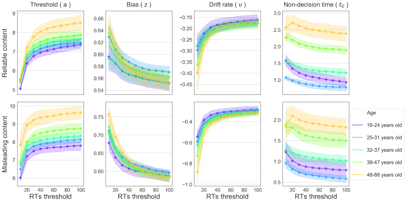
Here, we analyzed how the free parameters of the DDM vary as a function of the response time (RTs). For each threshold value, we consider those empirical responses corresponding to RTs lower than the threshold to then obtain the free parameters that better represent that pool of responses. As we can see, in both cases, misleading and reliable content, the values stabilized after $RTs=100$ . Each curve corresponds to a different age range, and for the sake of simplicity, we average among headlines.

Unbiased case of study

In this subsection, we explore the results of spreading (mis)information in a simple unbiased case. Within this context, individuals do not have a priori inclination. First, we obtain the expected fraction of individuals towards sharing information online $C_{SHARE}$ (See Methods) obtained with the estimated parameters (Fig. 5) for each age range and differentiating in the veracity of the content. As we can see from Fig. 2, people because more accurate with age, particularly for misleading content.

Second, we analyzed the theoretical phase diagram without bias exploring changes in the network structure. Fig. 3(a) corresponds to an Erdõs–Rényi (more homogeneous in degree), and Fig. 3(b) corresponds to a Power Law (more heterogeneous in degree).

From Fig. 3(b), we can see how the role of heterogeneity favors the virtualization of news headlines with “low quality” or unconvincing, having a wide spectrum depending on the $\gamma$ exponent. Yet, the role of the topology is not as impactful as the bias, for instance. Even for very heterogeneous networks, where heavily connected hubs are present and diffuse information rapidly through the entire network, results show that not every news headline will become viral. On the other hand, for more homogeneous networks Fig. 3(a), the topology does not play a crucial role; by increasing the average degree from $2$ to $10$ , the variance in the quality of the content in order to become viral does not change much.

Sensitivity analysis of the exponential cutoff on degree

Previous research [40, 52] has shown the absence of an epidemic threshold when pure power-law degree distributions with $2<\lambda<3$ are considered. For our purposes, this is a trivial case of study. Hence, we incorporate an exponential cutoff around the maximum degree $\kappa=10^{5}$ obtained in [39]. Additionally, here, we do a sensitivity analysis of the cutoff. As we can see in Fig. 4, low values of cutoff have a bigger impact on the free-parameters critical values, and as the cutoff increases, a steady behavior remains. This is due to the fact that the greater the cutoff, the closer the distribution is to the pure power-law behavior.

As a final step, we explore the case of Dunbar’s number $\kappa=150$ , suggested in [42] by analyzing Twitter data. We display the phase diagram in Supplementary Fig. 5, where the topology corresponds to Power Law network $P(k)\sim k^{-\gamma}\;exp(-k/\kappa)$ with $\gamma=2.2$ , cutoff on the degree of $\kappa=10^{5}$ (solid lines) and $\kappa=150$ (dashed lines).

Agent-based SIR model

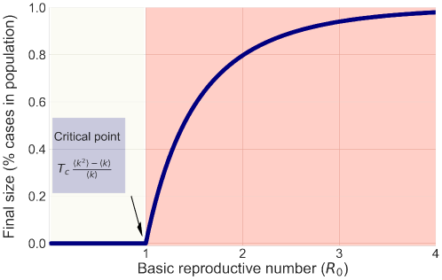
In this subsection, we display the final size of the population reached by the diseases as a function of $R_{0}$ in an epidemiological context; if we consider a misinformation context, it is the percentage of individuals that shared the content. The basic reproductive number $R_{0}$ is the expected number of cases originated by the first case (zero patient) in a population where all individuals are susceptible. Notice this assumes that no other individuals are infected or immunized. As we can see, for $R_{0}<1$ , the diseases vanishes. However, for $R_{0}>1$ , a macroscopic size of the population is reached by the diseases causing an epidemic scenario. From previous work [40, 51], we know the mathematical relationship in the critical point $R_{0}=1$ (Eq. within Fig. 6) between the contact patterns of a society (right side) and the characteristics of a disease (left side), $i.e.$ , we can determine if a specific emerging infectious disease will become an epidemic in a specific population.

Sensitivity analysis desegregating by headlines

Here, we display the probability distribution of response times for the empirical, theoretical, and simulated data. Each set of plots corresponds to a different headline and each plot to a different range of age.