Rainbow Hamiltonicity and the spectral radius

Abstract

Let $\mathcal{G}=\{G_{1},\ldots,G_{n}\}$ be a family of graphs of order $n$ with the same vertex set. A rainbow Hamiltonian cycle in $\mathcal{G}$ is a cycle that visits each vertex precisely once such that any two edges belong to different graphs of $\mathcal{G}$. We obtain a rainbow version of Ore’s size condition of Hamiltonicity, and pose a related problem. Towards a solution of that problem, we give a sufficient condition for the existence of a rainbow Hamiltonian cycle in terms of the spectral radii of the graphs in $\mathcal{G}$ and completely characterize the corresponding extremal graphs.

Keywords: Hamiltonicity, rainbow, spectral radius

AMS subject classification 2020: 05C50

1 Introduction

A graph $G$ is called Hamiltonian if it contains a cycle that visits each vertex of $G$ exactly once. Determining Hamiltonicity of graphs is an old and classic problem in graph theory, which is known to be NP-hard [18, pp. 85–103]. In 1952, Dirac [12] gave a sufficient condition in terms of the minimum degree, i.e., every graph $G$ with minimum degree at least $\tfrac{|V(G)|}{2}$ contains a Hamiltonian cycle. In 1960, Ore [23] extended Dirac’s condition and proved that every graph $G$ with $\sigma_{2}(G)\geq|V(G)|$ is Hamiltonian, where $\sigma_{2}(G)$ is the minimum degree sum among all pairs of nonadjacent vertices of $G$. These two conditions are respectively called Dirac-type condition and Ore-type condition. In 1961, Ore [24] showed another well-known condition in terms of the size (the number of edges $e(G)$ of $G$).

Theorem 1.1.

[24, Theorem 4.3] Let $G$ be a graph of order $n$. If $e(G)>\binom{n-1}{2}+1$, then $G$ is Hamiltonian.

Denote by $\vee$ and $\cup$ the join and union of two graphs, respectively. Ore [24] noted that his result is best possible in that $K_{1}\vee(K_{n-2}\cup K_{1})$ and $K_{2}\vee 3K_{1}$ are non-Hamiltonian and have exactly $\binom{n-1}{2}+1$ edges. Bondy [6] showed that these are the only extremal exceptional graphs.

Theorem 1.2.

[6, Theorem 1] Let $G$ be a graph of order $n$. If $e(G)\geq\binom{n-1}{2}+1$, then $G$ is Hamiltonian, unless $G\cong K_{1}\vee(K_{n-2}\cup K_{1})$ or $K_{2}\vee 3K_{1}$.

The adjacency matrix of $G$ with vertex set $V(G)$ and edge set $E(G)$ is defined as the matrix $A(G)=(a_{u,v})_{u,v\in V(G)}$ with $a_{u,v}=1$ if $uv\in E(G)$, and $a_{u,v}=0$ otherwise. The largest eigenvalue of $A(G)$, denoted by $\rho(G)$, is called the spectral radius of $G$. In 2010, Fiedler and Nikiforov [13] gave a sufficient condition for Hamiltonicity from a spectral perspective:

Theorem 1.3.

[13, Theorem 2] Let $G$ be a graph of order $n$. If $\rho(G)>n-2,$ then $G$ is Hamiltonian unless $G\cong K_{1}\vee(K_{n-2}\cup K_{1}).$

We note though that this result is weaker than Theorem 1.2, for it follows using Stanley’s inequality $e(G)\geq\rho(G)(\rho(G)+1)/2$ [25]. Let $\mathcal{G}=\{G_{1},\ldots,G_{n}\}$ be a family of graphs with the same vertex set $V$. Informally, we think of $G_{i}$ as a graph with edges that have color $i$. Now a graph $H$ is called rainbow in $\mathcal{G}$ if any two edges of $H$ belong to different graphs of $\mathcal{G}$; informally, any two edges have a different color.

For many famous results, rainbow versions have been considered, which led to beautiful results, such as rainbow versions for Carathéodory’s theorem [4], the Erdős–Ko–Rado theorem [3], Mantel’s theorem [1], and more [5, 11, 15, 17]. Also rainbow matchings have been considered. In particular, Guo et al. [14] obtained conditions in terms of the spectral radii for the existence of a rainbow matching.

In this paper, we let $H$ be a Hamiltonian cycle, and say that $\mathcal{G}$ is rainbow Hamiltonian if it admits such a rainbow Hamiltonian cycle. Here we assume that there are $n$ graphs in $\mathcal{G}$, each on the same vertex set of size $n$. Chen, Wang, and Zhao [7] obtained a rainbow version of Dirac’s theorem and showed that if each of the graphs $G_{i}\in\mathcal{G}$ has smallest degree are least $(1/2+o(1))n$, then $\mathcal{G}$ admits a rainbow Hamiltonian cycle. Joos and Kim [16] strengthened this result to smallest degree at least $n/2$. Li, Li, and Li [20] investigated the existence of a rainbow Hamiltonian path under an Ore-type condition: if $\sigma_{2}(G_{i})>n-2$ for all $i$, then $\mathcal{G}$ admits a rainbow Hamiltonian path [20, Theorem 1.3]. For other interesting results on rainbow Hamiltonian cycles and related problems we refer the reader to [2, 21, 22, 26].

In this paper, we consider rainbow versions of Theorems 1.1,1.2, and 1.3. We first obtain a rainbow version of Ore’s result in Theorem 3.1, thus obtaining a sufficient condition on the sizes of the graphs for the existence of a rainbow Hamiltonian cycle. We then pose the corresponding characterization of the extremal family of graphs (in terms of sizes) not admitting a rainbow Hamiltonian cycle as Problem 1. In order to work towards solving this problem, we obtain a sufficient condition on the spectral radii of the graphs for the existence of a rainbow Hamiltonian cycle, and characterize the extremal family of graphs in Theorem 4.3.

Our paper is further organized as follows: In Section 2, we describe the so-called Kelmans transformation, which is a well-known technique in extremal graph theory, and show that if a graph family is rainbow Hamiltonian after a Kelmans transformation, then it must be rainbow Hamiltonian itself (Lemma 2.4). In Section 3, we focus on conditions on the size of graphs, obtain a rainbow version of Theorem 3.1, and pose a rainbow version of Theorem 1.2 as a problem.

In Section 4, we obtain conditions on the spectral radii of graphs for the existence of a rainbow Hamiltonian cycle, and characterize the extremal graphs, thus obtaining a rainbow version of Theorem 1.3.

In the final section, we obtain a similar result in terms of the signless Laplacian spectral radii.

2 The Kelmans transformation

In extremal graph theory, one of the most important and widely used tools is the Kelmans transformation, as it controls efficiently many graph parameters. In this section we will state and prove some results about this transformation that are relevant to obtain our main results. For more about the Kelmans transformation, we refer the reader to [9, 19]. Let $x,y\in V(G)$, and let $N_{G}(x)$ and $N_{G}(y)$ denote the neighborhoods in $G$ of vertices $x$ and $y$, respectively.

Definition 2.1.

[19, Kelmans transformation] The Kelmans transformation on $G$ from $x$ to $y$ produces a new graph $\mathcal{K}_{xy}(G)$ by erasing all edges between $y$ and $N_{G}(y)\backslash(N_{G}(x)\cup\{x\})$ and adding all edges between $x$ and $N_{G}(y)\backslash(N_{G}(x)\cup\{x\})$.

Thus, the Kelmans transformation does not change the number of edges. However, it does affect the spectral radius $\rho(G)$.

Lemma 2.2.

[8, Theorem 2.1] Let $G$ be a graph and $x,y\in V(G)$. Then $\rho(\mathcal{K}_{xy}(G))\geq\rho(G)$.

Note that $\mathcal{K}_{xy}(G)\cong\mathcal{K}_{yx}(G)$, where we denote $G_{1}\cong G_{2}$ if $G_{1}$ and $G_{2}$ are isomorphic. We write $G_{1}=G_{2}$ if $V(G_{1})=V(G_{2})$ and $E(G_{1})=E(G_{2})$.

For a positive integer $n$, we use $[n]$ to denote the set $\{1,2,\ldots,n\}$. Let $G$ be a graph with vertex set $[n]$. Iterating the Kelmans transformation on $G$ for all vertex pairs $(x,y)$ satisfying $x<y$ will eventually produce a graph, denoted by $\mathcal{K}(G)$. Note that $N_{\mathcal{K}(G)}(y)\backslash\{x\}\subseteq N_{\mathcal{K}(G)}(x)\backslash\{y\}$ for each $x<y$. We will use this property mostly as follows.

Lemma 2.3.

Let $x<y$ and $z\neq x,y$. If $xz\notin E(\mathcal{K}(G))$, then $yz\notin E(\mathcal{K}(G))$.

Given a family $\mathcal{G}$, we let $\mathcal{K}_{xy}(\mathcal{G})=\{\mathcal{K}_{xy}({G}):G\in\mathcal{G}\}$ and $\mathcal{K}(\mathcal{G})=\{\mathcal{K}({G}):G\in\mathcal{G}\}.$ The next result shows that if the Kelmans transformed graph family $\mathcal{K}(\mathcal{G})$ is rainbow Hamiltonian then so is $\mathcal{G}$.

Lemma 2.4.

Let $\mathcal{G}=\{G_{1},G_{2},\ldots,G_{n}\}$ be a family of graphs on vertex set $[n]$. If $\mathcal{K}(\mathcal{G})$ admits a rainbow Hamiltonian cycle, then so does $\mathcal{G}$.

Proof.

It suffices to prove that for arbitrary vertices $x,y\in V(G)$, if $\mathcal{K}_{xy}(\mathcal{G})$ admits a rainbow Hamiltonian cycle, then so does $\mathcal{G}$. Let $C^{R}$ be a rainbow Hamiltonian cycle of $\mathcal{K}_{xy}(\mathcal{G})$ where $E(C^{R})=\{e_{i}:e_{i}\in\mathcal{K}_{xy}(G_{i}),1\leq i\leq n\}$.

Case 1.

$xy\in E(C^{R})$.

Suppose that $e_{i}=ux$ and $e_{j}=yv$ are two other edges in $C^{R}$. Because $v$ is a neighor of $y$ in ${K}_{xy}(G_{j})$, $v$ must be a common neighbor of $x$ and $y$ in both $\mathcal{K}_{xy}(G_{j})$ and $G_{j}$. Thus, $e_{j}=yv\in E(G_{j})$ and $xv\in E(G_{j})$. If $uy\in E(G_{i})$, then we find a rainbow Hamiltonian cycle of $\mathcal{G}$ by replacing $e_{i}$ and $e_{j}$ by $uy$ and $xv$ (see Fig. 1). If $uy\notin E(G_{i})$, then $ux\in E(G_{i})$ (otherwise, $u\notin N_{G_{i}}(x)$ and $u\notin N_{G_{i}}(y)$ and then $e_{i}=ux\notin E(\mathcal{K}_{xy}(G_{i}))$, a contradiction), so $C^{R}$ is also a rainbow Hamiltonian cycle of $\mathcal{G}$.

Case 2.

$xy\notin E(C^{R})$.

Let $e_{i}=a_{1}x$, $e_{i+1}=xa_{2}$, $e_{j}=b_{1}y$, and $e_{j+1}=yb_{2}$ be edges in $C^{R}$ (where $a_{1},a_{2},b_{1},$ and $b_{2}$ are not all necessarily distinct). Similar as in the above case, it follows that $b_{1}$ is a common neighbor of $x$ and $y$ in both $\mathcal{K}_{xy}(G_{j})$ and $G_{j}$, so that $b_{1}x,b_{1}y\in E(G_{j})$. Similarly, we have $xb_{2},yb_{2}\in E(G_{j+1})$.

Subcase 2.1.

$ya_{1}\notin E(G_{i})$.

If $ya_{1}\notin E(G_{i})$, then $a_{1}x\in E(G_{i})$ (otherwise $e_{i}=a_{1}x\notin E(\mathcal{K}_{xy}(G_{i}))$, a contradiction). (i) If $xa_{2}\in E(G_{i+1})$, then $C^{R}$ is a rainbow Hamiltonian cycle of $\mathcal{G}$; (ii) If $xa_{2}\notin E(G_{i+1})$, then $ya_{2}\in E(G_{i+1})$ (otherwise $e_{i+1}=xa_{2}\notin E(\mathcal{K}_{xy}(G_{i+1}))$, a contradiction), and we obtain a rainbow Hamiltonian cycle by replacing $e_{i+1}$ by $ya_{2}$ and $e_{j}$ by $b_{1}x$ (see Fig. 1).

Subcase 2.2.

$ya_{1}\in E(G_{i})$.

If $ya_{1}\in E(G_{i})$, then we first replace $e_{i}$ by $ya_{1}$ and $e_{j+1}$ by $xb_{2}$. (i) If $xa_{2}\in E(G_{i+1})$, then this gives a rainbow Hamiltonian cycle of $\mathcal{G}$ (see Fig. 1); (ii) If $xa_{2}\notin E(G_{i+1})$, then $ya_{2}\in E(G_{i+1})$ (as before) and we also replace $e_{i+1}$ by $ya_{2}$ and $e_{j}$ by $b_{1}x$ (see Fig. 1) to obtain also in this final case a rainbow Hamiltonian cycle of $\mathcal{G}$. ∎

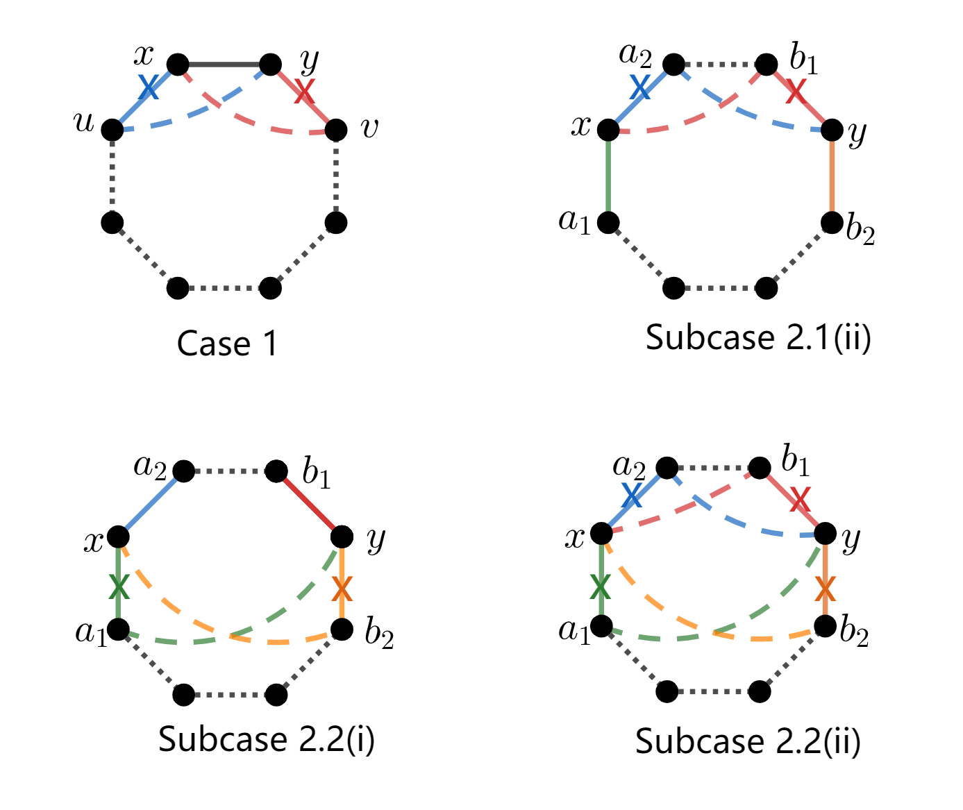
Figure 1: Switches in Lemma 2.4

We observe that the reverse of Lemma 2.4 does not necessarily hold. For example, the family of graphs $G_{1}=\cdots=G_{4}\cong C_{4}$ has a rainbow Hamiltonian cycle, but $\mathcal{K}(G_{1})=\cdots=\mathcal{K}(G_{4})\cong K_{1}\vee(K_{2}\cup K_{1})$ does not admit a rainbow Hamiltonian cycle.

3 Size conditions for rainbow Hamiltonicity

We are now ready to obtain our first main result, which is a sufficient condition in terms of the size for rainbow Hamiltonicity of a graph family; a rainbow version of Ore’s size condition (Theorem 1.1).

Theorem 3.1.

Let $n\geq 4$ and $\mathcal{G}=\{G_{1},G_{2},\ldots,G_{n}\}$ be a family of graphs on the same vertex set $[n]$, with

$$e(G_{i})>\binom{n-1}{2}+1,\mbox{\ for\ $i=1,2,\ldots,n.$}$$

Then $\mathcal{G}$ admits a rainbow Hamiltonian cycle.

Proof.

Assume (for a proof by contradiction) that $\mathcal{G}=\{G_{1},G_{2},\ldots,G_{n}\}$ does not admit a rainbow Hamiltonian cycle. Then by Lemma 2.4, the family $\mathcal{K}(\mathcal{G})$ does not admit a rainbow Hamiltonian cycle either, and

$$e(\mathcal{K}(G_{i}))=e(G_{i})>\binom{n-1}{2}+1\ \mbox{for $i=1,2,\ldots,n.$}$$

Let $e_{j}=\{j,n+2-j\}$ for $2\leq j\leq\lceil\tfrac{n}{2}\rceil$.

Claim 1.

$\{e_{3},\ldots,e_{\lceil\tfrac{n}{2}\rceil}\}\subseteq E(\mathcal{K}(G_{i}))$ for $i=1,2,\ldots,n$ (for $n\geq 5$).

Suppose that this claim does not hold, say $e_{j}\notin E(\mathcal{K}(G_{i}))$ for some $i,j$ with $3\leq j\leq\lceil\tfrac{n}{2}\rceil$ and $1\leq i\leq n$. Then it follows from Lemma 2.3 that if $z\geq j$ and $w\geq n+2-j$, then $\{z,w\}\notin E(\mathcal{K}(G_{i}))$. Thus $e(\mathcal{K}(G_{i}))\leq\binom{n}{2}-(n+2-2j)(j-1)-\binom{j-1}{2}\leq\binom{n-1}{2}+1$ (because $j\geq 3$ and $n\geq 5$), a contradiction. Thus, Claim 1 holds.

Let $e_{j}^{\prime}=\{j,n+1-j\}$ for $1\leq j\leq\lfloor\tfrac{n}{2}\rfloor$.

Claim 2.

$\{e_{1}^{\prime},\ldots,e_{\lfloor\tfrac{n}{2}\rfloor}^{\prime}\}\subseteq E(\mathcal{K}(G_{i}))$ for $i=1,2,\ldots,n.$

Indeed, it follows from Claim 1 and Lemma 2.3 that $e_{j}^{\prime}\in E(\mathcal{K}(G_{i}))$ for $j\geq 3$. In a similar way as in Claim 1, it can be shown that also $e_{1}^{\prime},e_{2}^{\prime}\in E(\mathcal{K}(G_{i}))$.

Claim 3.

$e_{2}\notin E(\mathcal{K}(G_{i}))$ for $i=1,2,\ldots,n.$

In order to prove this claim by contradiction, we assume that $e_{2}\in E(\mathcal{K}(G_{i}))$. Now it is relatively easy to construct a rainbow Hamiltonian cycle using this edge (with color $i$) and the edges $e_{j}$ $(3\leq j\leq\lceil\tfrac{n}{2}\rceil)$ and $e_{j}^{\prime}$ $(1\leq j\leq\lfloor\tfrac{n}{2}\rfloor)$ (all of which we can color as we wish because of Claims 1 and 2). In addition, we use an edge $\{j,1\}$ (which are edges in all $\mathcal{K}(G_{i})$ because $e_{1}^{\prime}$ is so). For $n$ even, the cycle (indicated by its edges for clarity) is

$$e_{2}\rightarrow e_{2}^{\prime}\rightarrow e_{3}\rightarrow e_{3}^{\prime}\rightarrow\cdots\rightarrow e_{\lceil\tfrac{n}{2}\rceil}\rightarrow e_{\lfloor\tfrac{n}{2}\rfloor}^{\prime}\rightarrow\{n+1-\lfloor\tfrac{n}{2}\rfloor,1\}\rightarrow e_{1}^{\prime}(\rightarrow e_{2}).$$

For $n$ odd, the cycle is

$$e_{2}\rightarrow e_{2}^{\prime}\rightarrow e_{3}\rightarrow e_{3}^{\prime}\rightarrow\cdots\rightarrow e_{\lceil\tfrac{n}{2}\rceil}\rightarrow\{\lceil\tfrac{n}{2}\rceil,1\}\rightarrow e_{1}^{\prime}(\rightarrow e_{2}).$$

Thus, we have a contradiction, and the claim is proven.

Now it follows from this last claim that vertex $n$ can only be adjacent to vertex $1$ in $\mathcal{K}(G_{i})$. Thus, the latter graph has at most $\binom{n-1}{2}+1$ edges, which is our final contradiction. ∎

Next, we would like to strengthen this result, and obtain a rainbow version of Theorem 1.2, by allowing $e(G_{i})\geq\binom{n-1}{2}+1$. For each $n\geq 6$, there is one exceptional graph, $K_{1}\vee(K_{n-2}\cup K_{1})$, that is not Hamiltonian, and hence the graph family $\mathcal{G}=\{G_{1},G_{2},\ldots,G_{n}\}$ with $G_{1}=\cdots=G_{n}\cong K_{1}\vee(K_{n-2}\cup K_{1})$ (see Fig 2) does not admit a rainbow Hamiltonian cycle.

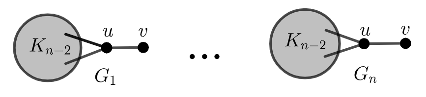
Figure 2: Graph family with $G_{1}=G_{2}=\cdots=G_{n}\cong K_{1}\vee(K_{n-2}\cup K_{1})$ that is not rainbow Hamiltonian.

Fortunately, any other graph family with graphs isomorphic to $K_{1}\vee(K_{n-2}\cup K_{1})$ is rainbow Hamiltonian, as we shall show next.

Lemma 3.2.

Let $n\geq 5$ and $\mathcal{G}=\{G_{1},G_{2},\ldots,G_{n}\}$ be a family of graphs of order $n$ on the same vertex set, where $G_{i}\cong K_{1}\vee(K_{n-2}\cup K_{1})$ for each $1\leq i\leq n$. Then $\mathcal{G}$ admits a rainbow Hamiltonian cycle unless $G_{1}=G_{2}=\cdots=G_{n}$.

Proof.

As remarked, if $G_{1}=G_{2}=\cdots=G_{n}$ then $\mathcal{G}$ is not rainbow Hamiltonian since $K_{1}\vee(K_{n-2}\cup K_{1})$ is not Hamiltonian. We assume now that the graphs in $\mathcal{G}$ are not equal and prove that $\mathcal{G}$ admits a rainbow Hamiltonian cycle. Let us denote the vertex degree of vertex $v$ in $G_{i}$ by $d_{i}(v)$. Suppose that $G_{1},\ldots,G_{n}$ have $k$ distinct vertices with degree $1$, and denote these $k$ distinct vertices by $v_{1},\ldots,v_{k}$. We distinguish the cases $k=1$ and $k\geq 2$.

We first give the proof for the case $k=1$. Then all graphs in $\mathcal{G}$ have $v_{1}$ with degree $1$. Without loss of generality, we assume that $G_{1}$ and $G_{2}$ are different. In this case, this means that the vertex that is adjacent to $v_{1}$ in $G_{1}$, $u_{1}$ say, and the one that is adjacent in $G_{2}$, $u_{2}$ say, are different. Since the graph induced on $V\backslash\{v_{1}\}$ in $G_{i}$ is the same $K_{n-1}$ for each $1\leq i\leq n$, it is clear that by using edges $v_{1}u_{1}$ in $G_{1}$ and $v_{1}u_{2}$ in $G_{2}$, we can make a rainbow Hamiltonian cycle in $\mathcal{G}$.

Next, we consider the case $k\geq 2$. Recall that $v_{1},\ldots,v_{k}$ are the $k$ distinct vertices with degree $1$ in $G_{1},\ldots,G_{n}$. Let

$$\mathcal{M}_{j}=\{G_{i}:d_{i}(v_{j})=1\}$$

and $m_{j}=|\mathcal{M}_{j}|$ for $1\leq j\leq k$. We let $m_{1}\leq m_{2}\leq\cdots\leq m_{k}$ by reordering vertices $v_{1},\ldots,v_{k}$ if necessary. Further, without loss of generality, we may assume that $\mathcal{M}_{1}=\{G_{1},\ldots,G_{m_{1}}\},$ $\mathcal{M}_{2}=\{G_{m_{1}+1},\ldots,G_{m_{1}+m_{2}}\},\ldots,$ $\mathcal{M}_{k}=\{G_{m-m_{k}+1},\ldots,G_{n}\}.$

Now we let $e_{i}=v_{i+1}v_{i+2}$, then it follows that $e_{i}\in E(G_{i})$ for each $1\leq i\leq n-2$, and hence these edges form a rainbow path $P_{n-2}^{R}$ (from $v_{2}$ to $v_{n}$) in $\{G_{1},\ldots,G_{n-2}\}$. We aim to construct a rainbow Hamiltonian cycle from this path by adding $v_{1}$ (on two edges, in $G_{n-1}$ and $G_{n}$) and replacing some edges. We will use that $d_{i}(v_{n})\neq 1$ for $1\leq i\leq n-1$ and $d_{n}(v_{1})\neq 1$ since $k\geq 2$.

We first claim that $v_{1}v_{n}\in E(G_{n-1})$, otherwise, we have $d_{n-1}(v_{1})=1$ because $d_{n-1}(v_{n})\neq 1$, which implies that $m_{1}=n-1$ and $m_{2}=1$, a contraction to $m_{1}\leq m_{2}$.

If $v_{1}v_{2}\in E(G_{n})$, then adding $e_{n-1}=v_{1}v_{n}$ and $e_{n}=v_{1}v_{2}$ to $P_{n-2}^{R}$ results in a rainbow Hamiltonian cycle in $\mathcal{G}$. Otherwise, we get $v_{1}v_{2}\notin E(G_{n})$, which implies that $d_{n}(v_{2})=1$, since $k\geq 2$. Therefore, $k=2$ and $m_{1}+m_{2}=n$. Because $m_{1}\leq m_{2}$, this implies that $m_{1}<n-1$. Note that $d_{m_{1}}(v_{1})=1$. Then $v_{2}v_{m_{1}+2}\in E(G_{m_{1}})$. Thus, except for the case $m_{1}=1$, we have $v_{1}v_{m_{1}+1}\in E(G_{n})$ since $d_{n}(v_{2})=1$. Adding $e_{n-1}=v_{1}v_{n}$ and $e_{n}=v_{1}v_{m_{1}+1}$, replacing $e_{m_{1}}=v_{m_{1}+1}v_{m_{1}+2}$ by $e_{m_{1}}^{\prime}=v_{2}v_{m_{1}+2}$ and leaving all other edges in $P_{n-2}^{R}$ results in a rainbow Hamiltonian cycle in $\mathcal{G}$ (see Fig. 3 (a)). For the remaining case ($m_{1}=1$ and $v_{1}v_{2}\notin E(G_{n})$), suppose that $v_{2}v_{j}\in E(G_{n})$ where $j\neq 1,2$. Adding $e_{n-1}=v_{1}v_{n}$ and $e_{n}=v_{2}v_{j}$, and replacing $e_{j-2}=v_{j-1}v_{j}$ by $e_{j-2}^{\prime}=v_{1}v_{j-1}$ and leaving all other edges in $P_{n-2}^{R}$ results in a rainbow Hamiltonian cycle in $\mathcal{G}$ (see Fig. 3 (b)). ∎

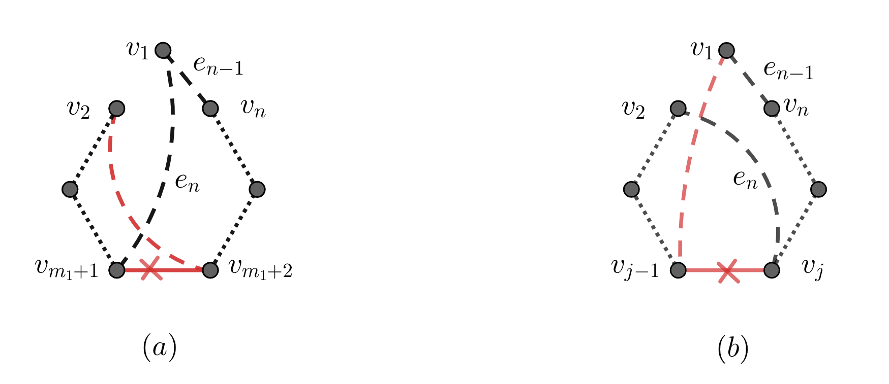
Figure 3: Rainbow Hamiltonian cycles in Lemma 3.2

We obtained a size condition of the rainbow Hamiltonicity of a graph family in Theorem 3.1 but did not characterize the extremal graphs. The reason is that the Kelmans transformation does not change the sizes of graphs, and we are not able to trace back the original graphs in $\mathcal{G}$ from $\mathcal{K}(G)$ by our approach. However, by Lemma 3.2, we have that $G_{1}=G_{2}=\cdots=G_{n}\cong K_{1}\vee(K_{n-2}\cup K_{1})$ gives an extremal graph family. Thus, we pose the following problem based on Theorems 1.2 and 3.1:

Problem 1.

Let $n\geq 6$ and $\mathcal{G}=\{G_{1},G_{2},\ldots,G_{n}\}$ be a family of graphs on the same vertex set $[n]$, with

$$e(G_{i})\geq\binom{n-1}{2}+1,\mbox{\ for\ $i=1,2,\ldots,n.$}$$

Does $\mathcal{G}$ admit a rainbow Hamiltonian cycle unless $G_{1}=G_{2}=\cdots=G_{n}\cong K_{1}\vee(K_{n-2}\cup K_{1})$ ?

One should remark that for $n=5$, the family $G_{1}=G_{2}=\cdots=G_{5}\cong K_{2}\vee 3K_{1}$ is clearly also not rainbow Hamiltonian.

4 Spectral radius conditions for rainbow Hamiltonicity

A possible step towards solving Problem 1 is to replace the size condition by a spectral condition and to obtain a rainbow version of the result by Fiedler and Nikiforov (Theorem 1.3). Indeed, recall from the introduction that if $\rho(G)>n-2$, then $e(G)\geq\binom{n-1}{2}+1$ by Stanley’s inequality. We note that the spectral radius of $K_{1}\vee(K_{n-2}\cup K_{1})$ is (just slightly) larger than $n-2$, because it has $K_{n-1}$ as a proper subgraph (and it is connected) [10, Prop. 1.3.10].

In order to obtain our main result of this section, we need the following lemmas.

Lemma 4.1.

Let $j\geq 3$ and $n\geq 2j-1$. Let $H_{j}\cong K_{j-1}\vee(K_{n+2-2j}\cup(j-1)K_{1})$. Then $\rho(H_{j})\leq n-2$ with equality only for $(n,j)=(5,3)$.

Proof.

The adjacency matrix of $H_{j}$ has an obvious equitable partition with three parts with corresponding quotient matrix

$$Q=\begin{bmatrix}j-2&n+2-2j&j-1\cr j-1&n+1-2j&0\cr j-1&0&0\cr\end{bmatrix}.$$

Let $\phi_{j}$ be the characteristic (cubic) polynomial of $Q$. Then $\phi_{j}(n-2)=\det((n-2)I-Q)=(n-2)(n-1)(j-2)-(2j-3)(j-1)^{2}\geq(2j-3)(j-1)(j-3)\geq 0$, with equality only for $(n,j)=(5,3)$. Unless $Q$ has two eigenvalues that are larger than $n-2$, this proves the statement. But the trace of $Q$ equals $n-1-j$, so two eigenvalues larger than $n-2$ would imply that the remaining eigenvalue, which is also an eigenvalue of $H_{j}$, is less than $-n$, which is impossible. ∎

We note that for $(n,j)=(5,3)$, the graph $H_{3}$ is the same as the exceptional non-Hamiltonian graph $K_{2}\vee 3K_{1}$ of Theorem 1.2.

Lemma 4.2.

Let $n\geq 4$ and $G^{*}\cong K_{1}\vee(K_{n-2}\cup K_{1})$. Then $\rho(G)\leq n-2$ for every proper subgraph $G$ of $G^{*}$, with equality only if $G\cong K_{n-1}$ or $G\cong K_{n-1}\cup K_{1}$.

Proof.

To show the bound, it suffices to show that it hold for graphs $G$ that are obtained from $G^{*}$ by deleting one edge. If this edge is incident with the vertex in $G^{*}$ that has degree $n-1$, then the maximum degree in $G$ is $n-2$, and hence it follows that $\rho(G)\leq n-2$, with equality only if $G$ has a regular component of degree $n-2$; in our case, if $G\cong K_{n-1}\cup K_{1}$. Further, it is clear that the only other subgraph of this graph with spectral radius $n-2$ is $K_{n-1}$. In any other case, deleting an edge from $G^{*}$ results in a graph that admits an equitable partition into four parts with quotient matrix

$$Q=\small{\begin{bmatrix}0&1&0&0\\ 1&0&2&n-4\\ 0&1&0&n-4\\ 0&1&2&n-5\end{bmatrix}},$$

that is, for $n\geq 5$ (the case $n=4$ gives $K_{1,3}$, with spectral radius $\sqrt{3}$). It is straightforward to check that if $\psi_{n}$ is the characteristic polynomial of $Q$, then $\psi_{n}(n-2)>0$ and $\psi_{n}(n-3)<0$. Because $\psi_{n}$ cannot have three roots larger than $n-3$ (similar as the argument in Lemma 4.1), this shows that $\rho(G)<n-2$. ∎

Now we have all the tools to extend the proof of Theorem 3.1 and show the following.

Theorem 4.3.

Let $n\geq 4$ and $\mathcal{G}=\{G_{1},G_{2},\ldots,G_{n}\}$ be a family of graphs on the same vertex set $[n]$, with

$$\rho(G_{i})>n-2,\mbox{\ for\ $i=1,2,\ldots,n.$}$$

Then $\mathcal{G}$ admits a rainbow Hamiltonian cycle unless $G_{1}=G_{2}=\cdots=G_{n}\cong K_{1}\vee(K_{n-2}\cup K_{1}).$

Proof.

We again write $G^{*}\cong K_{1}\vee(K_{n-2}\cup K_{1})$, and note that if $G_{1}=G_{2}=\cdots=G_{n}\cong G^{*}$, then $\mathcal{G}$ is not rainbow Hamiltonian.

Next, suppose that $\mathcal{G}$ is not rainbow Hamiltonian with $\rho(G_{i})>n-2$. We then aim to prove that $G_{1}=G_{2}=\cdots=G_{n}\cong G^{*}$. Indeed, by Lemma 2.4, $\mathcal{K}(\mathcal{G})$ does not admit a rainbow Hamiltonian cycle either and by Lemma 2.2, we have $\rho(\mathcal{K}(G_{i}))\geq\rho(G_{i})>n-2$ for each $i$. As before, we now let $e_{j}=\{j,n+2-j\}$ for $2\leq j\leq\lceil\tfrac{n}{2}\rceil$ and $e_{j}^{\prime}=\{j,n+1-j\}$ for $1\leq j\leq\lfloor\tfrac{n}{2}\rfloor$.

Claim 1.

$\{e_{3},\ldots,e_{\lceil\tfrac{n}{2}\rceil}\}\subseteq E(\mathcal{K}(G_{i}))$ for $i=1,2,\ldots,n$.

Indeed, if $e_{j}\notin E(\mathcal{K}(G_{i}))$ for some $i,j$ with $3\leq j\leq\lceil\tfrac{n}{2}\rceil$ and $1\leq i\leq n$, then it follows from Lemma 2.3 that if $z\geq j$ and $w\geq n+2-j$, then $\{z,w\}\notin E(\mathcal{K}(G_{i}))$, and hence $\mathcal{K}(G_{i})$ is a subgraph of $K_{j-1}\vee(K_{n+2-2j}\cup(j-1)K_{1})$. But then $\rho(\mathcal{K}(G_{i}))\leq\rho(K_{j-1}\vee(K_{n+2-2j}\cup(j-1)K_{1}))\leq n-2$, by Lemma 4.1, which is a contradiction. Thus, Claim 1 holds.

Claim 2.

$\{e_{1}^{\prime},\ldots,e_{\lfloor\tfrac{n}{2}\rfloor}^{\prime}\}\subseteq E(\mathcal{K}(G_{i}))$ for $i=1,2,\ldots,n$.

Indeed, it follows from Claim 1 and Lemma 2.3 that $e_{j}^{\prime}\in E(\mathcal{K}(G_{i}))$ for $j\geq 3$. If $e_{1}^{\prime}=\{1,n\}\notin E(\mathcal{K}(G_{i}))$, then $n$ is an isolated vertex, and hence $\mathcal{K}(G_{i})$ is a subgraph of $K_{n-1}\cup K_{1}$, which has spectral radius $n-2$, a contradiction. If $e_{2}^{\prime}=\{2,n-1\}\notin E(\mathcal{K}(G_{i}))$, then it follows that $\mathcal{K}(G_{i})$ is a subgraph of $K_{1}\vee(K_{n-3}\cup 2K_{1})$, which has spectral radius smaller than $n-2$ (which can be shown in a similar way as Lemma 4.1), again a contradiction. Thus, also Claim 2 holds.

Claim 3.

$e_{2}\notin E(\mathcal{K}(G_{i}))$ for $i=1,2,\ldots,n$.

The proof of this claim is exactly the same as in the proof of Theorem 3.1, and as before, it follows that vertex $n$ can only be adjacent to vertex $1$ in $\mathcal{K}(G_{i})$. Thus, $\mathcal{K}(G_{i})$ is a subgraph of $G^{*}\cong K_{1}\vee(K_{n-2}\cup K_{2})$. Because $\rho(\mathcal{K}(G_{i}))>n-2$, it then follows from Lemma 4.2 that $\mathcal{K}(G_{i})\cong G^{*}$, for each $i$. Finally, by Lemma 3.2, we then have that $G_{1}=\cdots=G_{n}\cong G^{*}.$ ∎

5 The signless Laplacian spectral radius

The signless Laplacian matrix of $G$ is defined as $S(G)=D(G)+A(G)$, where $D(G)$ is the diagonal matrix of vertex degrees of $G$. The largest eigenvalue of $S(G)$, denoted by $\rho_{S}(G)$, is called the signless Laplacian spectral radius of $G$. Note that $S(G)=2A(G)+L(G)$, where $L(G)$ is the usual Laplacian matrix, which is positive semidefinite. Hence $\rho_{S}(G)\geq 2\rho(G)$.

Yu and Fan [27] observed that Theorem 1.3 has a (slightly stronger) analogue in terms of the signless Laplacian spectral radius. They showed that $\rho_{S}(G)>2n-4$ implies that $e>\binom{n-1}{2}$, and hence they obtained the following from Theorem 1.2.

Theorem 5.1.

[27, Theorem 4.1] Let $n\geq 6$ and $G$ be a graph of order $n$. If $\rho_{S}(G)>2n-4,$ then $G$ is Hamiltonian unless $G\cong K_{1}\vee(K_{n-2}\cup K_{1}).$

We note that $n=5$ is again excluded, because the non-Hamiltonian graph $K_{2}\vee 3K_{1}$ has signless spectral radius larger than 6.

A rainbow version of this result is now easily obtained by adjusting our proof of Theorem 4.3 (and the underlying lemmas) to the signless spectral radius.

Theorem 5.2.

Let $n\geq 6$ and $\mathcal{G}=\{G_{1},G_{2},\ldots,G_{n}\}$ be a family of graphs on the same vertex set $[n]$ with

$$\rho_{S}(G_{i})>2n-4,\mbox{\ for\ $i=1,2,\ldots,n.$}$$

Then $\mathcal{G}$ admits a rainbow Hamiltonian cycle unless $G_{1}=G_{2}=\cdots=G_{n}\cong K_{1}\vee(K_{n-2}\cup K_{1}).$

References

- [1] R. Aharoni, M. DeVos, S. G. H. de la Maza, A. Montejano, and R. Šámal. A rainbow version of Mantel’s theorem. Advances in Combinatorics, 2:12pp, 2020.
- [2] R. Aharoni, R. Holzman, and Z. Jiang. Rainbow fractional matchings. Combinatorica, 39(6):1191–1202, 2019.
- [3] R. Aharoni and D. Howard. A rainbow -partite version of the Erdős–Ko–Rado theorem. Combinatorics, Probability and Computing, 26(3):321–337, 2017.
- [4] I. Bárány. A generalization of Carathéodory’s theorem. Discrete Mathematics, 40(2-3):141–152, 1982.
- [5] B. Bollobás, P. Keevash, and B. Sudakov. Multicoloured extremal problems. Journal of Combinatorial Theory, Series A, 107(2):295–312, 2004.
- [6] J. A. Bondy. Variations on the hamiltonian theme. Canadian Mathematical Bulletin, 15(1):57–62, 1972.
- [7] Y. Cheng, G. Wang, and Y. Zhao. Rainbow pancyclicity in graph systems. The Electronic Journal of Combinatorics, 28(#P3.24):141–152, 2021.
- [8] P. Csikvári. On a conjecture of V. Nikiforov. Discrete Mathematics, 309(13):4522–4526, 2009.
- [9] P. Csikvári. Applications of the Kelmans transformation: extremality of the threshold graphs. The Electronic Journal of Combinatorics, 18(1):P182, 2011.
- [10] D. Cvetković, P. Rowlinson, and S. Simić. An introduction to the theory of graph spectra. Cambridge University Press, 2009.
- [11] S. Das, C. Lee, and B. Sudakov. Rainbow Turán problem for even cycles. European Journal of Combinatorics, 34(5):905–915, 2013.
- [12] G. A. Dirac. Some theorems on abstract graphs. Proceedings of the London Mathematical Society, 3(1):69–81, 1952.
- [13] M. Fiedler and V. Nikiforov. Spectral radius and Hamiltonicity of graphs. Linear Algebra and Its Applications, 9(432):2170–2173, 2010.
- [14] M. Guo, H. Lu, X. Ma, and X. Ma. Spectral radius and rainbow matchings of graphs. Linear Algebra and its Applications, 679:30–37, 2023.
- [15] A. F. Holmsen, J. Pach, and H. Tverberg. Points surrounding the origin. Combinatorica, 28(6):633–644, 2008.
- [16] F. Joos and J. Kim. On a rainbow version of Dirac’s theorem. Bulletin of the London Mathematical Society, 52(3):498–504, 2020.
- [17] G. Kalai and R. Meshulam. A topological colorful Helly theorem. Advances in Mathematics, 191(2):305–311, 2005.
- [18] R. M. Karp. Reducibility among combinatorial problems. Complexity of Computer Computations. New York: Plenum Press, 1972.
- [19] A. K. Kelmans. On graphs with randomly deleted edges. Acta Mathematica Academiae Scientiarum Hungaricae, 37:77–88, 1981.
- [20] L. Li, P. Li, and X. Li. Rainbow structures in a collection of graphs with degree conditions. Journal of Graph Theory, pages 1–19, 2023.
- [21] H. Lu, X. Yu, and X. Yuan. Rainbow matchings for 3-uniform hypergraphs. Journal of Combinatorial Theory, Series A, 183:105489, 2021.
- [22] R. Montgomery, A. Müyesser, and Y. Pehova. Transversal factors and spanning trees. Advances in Combinatorics, 3:5, 2020.
- [23] O. Ore. A note on hamiltonian circuits. American Mathematical Monthly, 67:55, 1960.
- [24] O. Ore. Arc coverings of graphs. Annali di Matematica Pura ed Applicata, 55(1):315–321, 1961.
- [25] R. P. Stanley. A bound on the spectral radius of graphs with edges. Linear Algebra and Its Applications, 87:267–269, 1987.
- [26] Y. Tang, B. Wang, G. Wang, and G. Yan. Rainbow Hamilton cycle in hypergraph system. arXiv preprint arXiv:2302.00080, 2023.
- [27] G. Yu and Y. Fan. Spectral conditions for a graph to be Hamilton-connected. Applied Mechanics and Materials, 336:2329–2334, 2013.