Privacy-preserving data release leveraging optimal transport
and particle gradient descent

Abstract

We present a novel approach for differentially private data synthesis of protected tabular datasets, a relevant task in highly sensitive domains such as healthcare and government. Current state-of-the-art methods predominantly use marginal-based approaches, where a dataset is generated from private estimates of the marginals. In this paper, we introduce PrivPGD, a new generation method for marginal-based private data synthesis, leveraging tools from optimal transport and particle gradient descent. Our algorithm outperforms existing methods on a large range of datasets while being highly scalable and offering the flexibility to incorporate additional domain-specific constraints.

1 Introduction

Distributing sensitive datasets is crucial for data-driven decision-making and methodological research in many fields, including healthcare and government. For example, epidemiologists and biostatisticians have relied on tools like SAS to analyze personal health data for decades [13, 10]. However, there are significant concerns among patients about the use and disclosure of their information, especially among vulnerable groups [19].

Differential privacy (DP) has gained prominence as a vital approach to mitigate privacy concerns. Its adoption extends well beyond theoretical frameworks, finding practical utility across industries and government organizations [25, 1, 2]. In this paper, we target the problem of differentially private tabular data synthesis, a promising approach for creating high-quality copies of protected tabular datasets that adhere to privacy constraints. Any further task performed on these “private” copies is thus guaranteed to comply with these constraints.

Numerous differential privacy methods have emerged to synthesize tabular datasets with privacy guarantees while preserving relevant statistics from the original dataset [24, 40]. Marginal-based approaches are among the preferred methods, dominant in NIST challenges [35] and consistently top-ranked in benchmarks [40]. These approaches select a set of marginals and perturb them in a DP-compliant manner. Subsequently, a synthetic dataset is generated from these noisy marginals through a generation method.

In this paper, we introduce PrivPGD, a novel DP-data generation method based on particle gradient descent. PrivPGD leverages an optimal transport-based divergence between the privatized and particle marginal distributions (Section 2.2) to effectively integrate marginal information during gradient descent. This divergence can be approximated highly efficiently through parallel GPU processing, which is crucial for handling large datasets. Our approach has several important characteristics:

• State-of-the-Art performance. PrivPGD outperforms state-of-the-art methods in a large benchmark comparison (9 datasets) across a wide range of metrics, including downstream task performance (Section 4).

• Scalability. PrivPGD leverages a highly optimized gradient computation that can be parallelized on GPU, enabling the algorithm to efficiently construct large datasets with over 100,000 data points while accommodating many marginals, e.g., all 2-Way marginals.

• Geometry preservation. Many datasets contain features with inherent geometry, such as continuous features and some categorical features like age, which have rankings that should be retained in the synthetic data. Unlike state-of-the-art methods (see Section 4.2), PrivPGD preserves this geometric structure, aligning more naturally with the nuances of real-world datasets.

• Incorporation of domain-specific constraints. Since PrivPGD is a gradient-based method, we can include any additive penalization term to the loss function. This way, we can explicitly enforce the generation algorithm to respect additional domain-specific constraints and thereby offer a simple and efficient way to incorporate requirements in the synthetic data.

1.1 Related work

We discuss in this section related works on DP-data synthesis for tabular data and refer the reader to Section 4 for an extensive benchmark comparison (for a more comprehensive overview, see the recent survey [24]). We distinguish between marginal and query-based DP-data synthesis algorithms. While the latter receives any general set of queries and releases a tabular dataset that simultaneously answers all queries, the former only considers marginal queries and can thus be viewed as a special case of query-based algorithms, optimized for marginal queries.

Marginal-based algorithms

Marginal-based algorithms are prominent in the literature for private tabular data release, achieving state-of-the-art performance on numerous benchmark tasks [35, 24, 40]. These algorithms comprise two main steps: the selection of marginals [35, 36, 8] and the dataset generation after adding noise to the selected marginals [34, 51, 30]. A common approach in data generation is PGM, used by winning methods in the NIST competitions [35, 36, 8]. However, PGM faces two major limitations: it is highly sensitive to the number of selected marginals, easily resulting in memory and runtime issues, and has limited capability in preserving domain-specific constraints. Other marginal-based generation methods include PrivBayes [51], where a Bayesian Neural Network is trained, and Gradual Update Methods (GUM) [30, 52], which initialize a random dataset and iteratively update it to match the marginals.

Query-based algorithms

In contrast to marginal-based algorithms, which can only preserve marginal-based queries, query-based algorithms can handle a broader range of queries. Some examples include DualQuery [20], FEM [44], RAP [4], GEM [32], RAP++ [45], Private GSD [33], and others [46, 31]. These methods construct a private dataset to efficiently answer a large set of pre-defined queries simultaneously, often relying on gradient descent techniques [4, 32]. While our method, PrivPGD, also uses particle gradient descent, unlike previous approaches, it does not require predefining a set of queries and is optimized for preserving marginal queries.

Other algorithms

Copula-based approaches [21, 29, 3] employ Gaussian and vine copulas to approximate the privatized marginal distributions. However, such approaches suffer from high computational complexity, limiting their applicability. For instance, running a single iteration of Copula-Shirley [21] on the ACS datasets [14] takes over 24 hours on our cluster. Furthermore, while Generative Adversarial Networks (GANs) have been proposed for synthesising private data [26, 41, 48, 43], these methods reportedly fail to preserve basic distributional statistics for tabular datasets [40]. DP-Sinkhorn [9], another optimal transport-based generative method, cannot be easily extended to tabular data synthesis. Finally, projection-based methods struggle to model complex relationships [49, 27].

2 Preliminaries for differentially private data synthesis

In this section, we summarize key concepts and introduce notation related to differentially private data synthesis used in the paper.

In general, we consider our data to lie in a domain $\mathcal{X}=\mathcal{X}_{1}\times\cdots\times\mathcal{X}_{d}$ that is discrete and has dimension $d$. This assumption is not restrictive since the vast majority of DP-data synthesis algorithms for tabular data rely on a discretized version of the data even if it originally lies in a continuous domain. In particular, we can represent every dimension as an integer in the discrete set $\mathcal{X}_{i}=\{1,\cdots,k_{i}\}$ with $k_{i}\in\mathbb{N}_{+}$.

Differential privacy [16] is an algorithmic property that guarantees that individual information in the data is protected in the output of an algorithm; even when assuming that an adversary has access to the information of all other individuals in the dataset. We now provide the formal definition.

Definition 1

An algorithm ${\mathcal{A}}$ is $(\epsilon,\delta)$-DP with $\epsilon>0$ and $\delta>0$ if for any datasets $D,D^{\prime}$ differing in a single entry and any measurable subset $S\subset\mathrm{im}(\mathcal{A})$ of the image of $\mathcal{A}$, we have

$$\mathbb{P}\left(\mathcal{A}\left(D\right)\in S\right)\leq\exp(\epsilon)\mathbb{P}\left(\mathcal{A}\left(D^{\prime}\right)\in S\right)+\delta$$

The goal of differentially private data synthesis is to design a (randomized) algorithm ${\mathcal{A}}$ that, for any dataset $D\in\mathcal{X}^{n}$ of size $n$, generates an output $\mathcal{A}\left(D\right)\in\mathcal{X}^{m}$ that is a differentially private “copy” of $D$, potentially of different size $m\neq n$.

2.1 Marginal-based algorithms for private data synthesis

Our approach falls in the general category of marginal-based methods. They follow Algorithm 1, consisting of three steps: marginal selection, privatization, and generation.

Marginal selection

For any subset $S\subset\{1,\cdots,d\}$ of the dimensions, we denote with $D_{S}\in\mathcal{X}_{S}^{n}$ the dataset containing only the dimensions in $S$. For each subset $S$ we can define a corresponding marginal.

Definition 2

We denote by $\nu_{S}[D]\in\mathcal{P}(\mathcal{X}_{S})$ the $S$-marginal of a dataset $D$, defined as the empirical measure of $D_{S}$ over the domain $\mathcal{X}_{S}$.

In the first step of the algorithm, a set $\mathcal{S}$ of such subsets $S$ is selected, and equivalently a set of marginals. The problem of selecting marginals in a DP-way is an interesting problem on its own and has led to a significant amount of proposed methods [8, 35, 36, 52]. In an extension of Algorithm 1, sketched in Algorithm 2, the marginals are not all selected in the beginning, but sequentially chosen from a pre-defined pool of subsets $\mathcal{S}_{W}$ of $[d]$ (often referred to as the workload). More specifically, in every iteration $t$, we select the marginals with the largest total variation distance $\text{TV}\left(\nu_{S}[D_{\text{DP}}^{(t-1)}],\nu_{S}[D]\right)$, where $D_{\text{DP}}^{(t-1)}$ is the DP-dataset from the previous iteration $t-1$. This is done in a DP-way using the exponential mechanism [37]. Such approaches fall under the general MWEM [23, 32] framework, which is the backbone of many DP synthesis methods. To control the overall privacy budget, the framework from Algorithm 2 uses advanced compositional theorems (see e.g., [18]).

Algorithm 1 Standard data synthesis framework

1:Dataset $D$, privacy parameters $\epsilon$ and $\delta$

2:select set $\mathcal{S}$ of subsets $S$ of $\{1,\cdots,d\}$

3:privatize marginals $\nu_{S}[D]$ to obtain $(\epsilon,\delta)$-DP “copies” $\hat{\nu}_{S}$

4:generate data from privatized marginals $\hat{\nu}_{S}$

5:return the DP dataset $D_{\text{DP}}$

Algorithm 2 Extension to sequential query selection

1:Dataset $D$, privacy parameters $\epsilon$ and $\delta$, workload $\mathcal{S}_{W}$, rounds $T$

2:for $t=1,\dots,T$ do

3:     select $S_{t}\in\mathcal{S}_{W}$

4:     privatize the marginal $\nu_{S_{t}}[D]$ to obtain the

5:          DP-“copies” $\hat{\nu}_{S_{t}}$

6:     generate data from privatized marginals

7:          $\{\hat{\nu}_{S_{j}}\}_{j\leq t}$ to obtain $D^{(t)}_{DP}$

8:end for

9:return DP dataset $D^{(T)}_{DP}$.

Marginal privatization

After a set of marginals has been selected, both frameworks contain a privatization and generation step. A common choice for privatization is to apply the Gaussian mechanism [37], where we simply add i.i.d. Gaussian noise to the empirical marginal $\nu_{S}[D]$. The variance $\sigma^{2}$ of the Gaussian depends on the privacy parameters $\epsilon$ and $\delta$. As a result, we obtain the signed measures $\hat{\nu}_{S}$:

$$\forall x\in\mathcal{X}_{S}:~{}~{}\hat{\nu}_{S}(\{x\})=\nu_{S}[D](\{x\})+\mathcal{N}(0,\sigma^{2}).$$

Data generation

Finally, in the last step, we generate a dataset from the noisy estimates of the marginals. For this purpose, existing methods typically aim to learn a distribution $\hat{p}$ that minimizes the squared loss:

$$\sum_{S\in\mathcal{S},x\in\mathcal{X}_{S}}\left(\hat{p}_{S}(\{x\})-\hat{\nu}_{S}(\{x\})\right)^{2}$$

and then release the private synthetic data $D_{\text{DP}}$ by sampling from $\hat{p}$. The predominant generation algorithm used by state-of-the-art methods [35, 36, 8] is PGM [34], which learns a graphical model using mirror descent. We refer to Section 1.1 for further discussion.

2.2 Sliced Wasserstein distance

The optimal transport literature offers a set of natural divergence measures that can be used for particle gradient descent, such as the Sinkhorn divergence or the Wasserstein distance. However, the computational complexity of these divergences scales at least quadratically (resp. cubically) with respect to the size of the support of the measures. This clearly defeats the purpose of a computationally efficient generation algorithm that can represent rich datasets with a large number of data points. Instead, a widely used [47, 28, 11, 12], computationally efficient alternative is the squared sliced Wasserstein ($\text{SW}_{2}^{2}$) distance [6]; that is, the averaged squared Euclidean transportation over all $1$-dimensional projections.

Formally, for $\theta\in\mathbb{R}$, let $g^{\theta}(x)=\langle x,\theta\rangle$ and $g^{\theta}_{\#}$ be the pullback measure induced by $g^{\theta}$. Moreover, let $\lambda^{p}$ be the uniform distribution over the sphere $\mathcal{S}^{p-1}$. For any Euclidean subspace $\Omega\subset\mathbb{R}^{p}$ and probability measures $\mu,\nu\in\mathcal{P}(\Omega)$ with support $\Omega$, the $q$-SW distance is defined as follows:

$$\text{SW}_{q}(\mu,\nu)=\left(\int_{\mathcal{S}^{p-1}}W_{q}^{q}(g^{\theta}_{\#}\mu,g^{\theta}_{\#}\nu)d\lambda(\theta)\right)^{1/q},$$ (1)

where $W_{q}^{q}$ is the $q$-th power of the $q$-Wasserstein distance for $q\geq 1$. The Wasserstein distance over $1$-dimensional distributions, as it appears in Equation 1, has a well-known closed-form expression:

$$W_{q}(g^{\theta}_{\#}\mu,g^{\theta}_{\#}\nu)=\left(\int_{u}|F^{-1}_{g^{\theta}_{\#}\mu}(u)-F^{-1}_{g^{\theta}_{\#}\nu}(u)|^{q}du\right)^{1/q},$$ (2)

where $F_{g^{\theta}_{\#}\mu}(u)$ (resp. $F_{g^{\theta}_{\#}\nu}(u)$) represents the cumulative function and $F^{-1}$ its inverse. Finally, in the special case of $q=1$, we have the following identity for the $1$-Wasserstein distance by Vallender [42], which we will later leverage in our algorithm:

$$W_{1}(g^{\theta}_{\#}\mu,g^{\theta}_{\#}\nu)=\|F_{g^{\theta}_{\#}\mu}(u)-F_{g^{\theta}_{\#}\nu}(u)\|_{L_{1}(\mathbb{R})}.$$ (3)

Importantly, this identity allows us to naturally extend the definition of the (sliced) $1$-Wasserstein distance to signed measures, as demonstrated by Boedihardjo et al. [5].

3 PrivPGD: a particle gradient descent-based generation method

We introduce PrivPGD (Algorithm 3), a novel approach for solving the generation step in marginal-based tabular data synthesis (Algorithm 1). Unlike other marginal-based methods [51, 34], PrivPGD does not construct a dataset by sampling from a learned distribution. Instead, it directly propagates particles in an embedding space to minimize the sliced Wasserstein distance. A distinct advantage is that, through particle gradient descent, we can easily enforce domain-specific constraints by adding a penalization term $\hat{\mathcal{R}}$ to the loss. A similar approach for incorporating domain-specific constraints has recently been proposed for GAN-based data synthesis algorithms [43], where the authors provide various examples of such losses.

In summary, our data generation method returns a DP-dataset $D_{\text{DP}}$ given the following inputs:

1. A set of differentially private finite signed measures $\{\hat{\nu}_{S}\}_{S\in\mathcal{S}}$ constructed as in Algorithm 1.

2. A differentially private regularization loss $\hat{\mathcal{R}}$ incorporating domain-specific constraints.

3.1 Preliminaries: Embedding

PrivPGD crucially relies on an embedding ${\text{Emb}:\mathcal{X}\to\Omega}$ of the (discretized) domain $\mathcal{X}$ into a compact Euclidean product space $\Omega=\Omega_{1}\times\cdots\times\Omega_{d}$. We simply choose $\Omega=[0,1]^{d}$ and map every $x\in\mathcal{X}$ to equally-spaced centers

$$\text{Emb}(x)_{i}=\frac{2x_{i}-1}{2k_{i}}\in[0,1].$$ (4)

This choice of embedding preserves the order in $\mathcal{X}$, which is essential for variables such as age or any discretized continuous variables. In line with common practices in the literature [35, 40], we discretize continuous data using equally spaced bins. This method ensures that the embedding accurately represents the scaled distances between the centers.

We acknowledge that for features like race, where imposing an ordering might be inappropriate, these could be embedded into the space $[0,1]^{2}$ in a way that ensures the centers are equidistant. Similarly, when embedding categorical variables representing locations, an embedding that preserves geographical distances might be preferable. While it would be interesting to explore other embeddings, we leave it to future work.

Particles

PrivPGD aims to construct $m$ data points in the embedding space, ensuring their empirical distribution closely approximates the projection of the privatized signed measure $\hat{\nu}_{S}$. For any set of points $Z\in\Omega^{m}$, which we also refer to as the $m$ particles, we define $Z_{S}\in\Omega_{S}^{m}$ as the projection of these particles onto the embedding $\Omega_{S}$ of $\mathcal{X}_{S}$. Moreover, we define $S$-marginals over $\Omega$ as:

Definition 3

We denote by $\mu_{S}[Z]\in\mathcal{P}(\Omega_{S})$ the $S$-marginal of the particles $Z$, defined as the empirical measure of $Z_{S}$ over the domain $\Omega_{S}$.

Algorithm 3 Private Particle Gradient Descent

1:DP marginals $\{\hat{\nu}_{S}\}_{S\in\mathcal{S}}$, regularizer $\hat{\mathcal{R}}$ , number of particles $m$

2:projection: $\forall S\in\mathcal{S}$, construct the empirical measures $\hat{\mu}_{S}$ from $\hat{\nu}_{S}$

3:optimization: randomly initialize $Z^{(0)}\in\Omega^{m}$

4:for $t=1,\cdots,T$ do

5:     select batch $\mathcal{S}_{\text{batch}}\subset\mathcal{S}$

6:     compute the gradient at $Z^{(t-1)}$ of $\sum_{S\in\mathcal{S}_{\text{batch}}}\text{SW}_{2}^{2}(\mu_{S}[Z],\hat{\mu}_{S})+\lambda\hat{\mathcal{R}}(Z)$

7:     update $Z^{(t)}$ using any first order optimizer

8:end for

9:finalization step: construct $D_{\text{DP}}$ from $Z^{(T)}$

10:return $D_{\text{DP}}$

3.2 Projection step

The preliminary embedding step allows us to define the particles $Z$ within a convenient domain $\Omega$, which we choose to be the hypercube with a fixed grid. In the projection step, the goal is to transform the privatized signed measure $\hat{\nu}_{S}$ into a proper probability measure $\hat{\mu}_{S}$ that can be “plugged into” the Wasserstein distance. Further, since we aim to find particles whose empirical distribution closely approximates the signed measure, we quantize $\hat{\mu}_{S}$ using the same number of particles, $m$.

Projection

First, note that the embedding Emb from Equation 4 defines corresponding finite signed measures $\hat{\omega}_{S}$ over $\text{Emb}(\mathcal{X})_{S}\subset\Omega_{S}$ for each privatized signed measure $\hat{\nu}_{S}$. By default, the sliced Wasserstein distance that we minimize in the optimization step (Section 3.3) is defined for probability measures. For $q=1$ we can extend the sliced 1-Wasserstein distance from Equation 3 to signed measures and obtain a probability measure. Inspired by Boedihardjo et al. [5] (see also [15]), we transform by solving

$$\hat{\omega}_{S,\mathbb{P}}=\arg\min_{w\in\mathcal{P}(\text{Emb}(\mathcal{X})_{S})}\text{SW}_{1}(w,\hat{\omega}_{S}).$$ (5)

We approximate this convex optimization problem using gradient descent. We also approximate the integral in $\text{SW}_{1}$ using Monte Carlo samples. Importantly, minimizing the objective in Equation 5 allows for preserving the geometry from the signed measures in the probability measures.

Quantization

We further quantize the finite probability measures $\hat{\omega}_{S,\mathbb{P}}$ using $m$ particles $\hat{Z}_{S}\in\Omega^{m}_{S}$, i.e.,

$$\hat{\mu}_{S}=\frac{1}{m}\sum_{i=1}^{m}\delta[\hat{Z}_{S}^{i}],$$ (6)

such that $\hat{\mu}_{S}\approx\hat{\omega}_{S,\mathbb{P}}$. This can be achieved by using any standard quantization technique with a negligible error for a sufficiently large number of particles. We apply the quantization in Equation 6 with $m$ particles, thus ensuring that both $\mu_{S}[Z]$ and $\hat{\mu}_{S}$ are empirical measures over the same number of particles.

3.3 Optimization and finalization step

In the optimization step, we aim to generate a dataset by finding particles $Z\in\Omega^{m}$ that are close to the differentially private measure $\hat{\mu}_{S}$ constructed in the projection step. In particular, the final particles should minimize the squared sliced Wasserstein distance $\text{SW}_{2}^{2}$ (Equation 1) between the empirical marginal distributions of the particles $\mu_{S}[Z]$ and $\hat{\mu}_{S}$. We additionally incorporate domain-specific constraints via a DP differentiable penalty term $\hat{\mathcal{R}}:\Omega^{m}\to\mathbb{R}$. Formally, for a regularization strength $\lambda$, we run mini-batch particle gradient descent on

$$\mathcal{L}_{\mathcal{S}}(Z):=\sum_{S\in\mathcal{S}}\text{SW}_{2}^{2}(\mu_{S}[Z],\hat{\mu}_{S})+\lambda\hat{\mathcal{R}}(Z),$$ (7)

where $\text{SW}_{2}^{2}$ is the squared sliced Wasserstein distance.

Computing the gradient of the $\text{SW}_{2}^{2}$ distance

For computing the gradient, we leverage the fact that the 1-dimensional $2$-Wasserstein distance between $g^{\theta}_{\#}\mu_{S}[Z]=\frac{1}{m}\sum_{i}\delta(y_{i})$ and $g^{\theta}_{\#}\hat{\mu}_{S}=\frac{1}{m}\sum_{i}\delta(y^{\prime}_{i})$ with $y_{i},y^{\prime}_{i}\in\mathbb{R}$ has a closed-form expression

$$W_{2}^{2}(g^{\theta}_{\#}\mu_{S}[Z],g^{\theta}_{\#}\hat{\mu}_{S})=\frac{1}{m}\sum_{i}(y_{[i]}-y^{\prime}_{[i]})^{2},$$ (8)

where $y_{[i]}$ (resp. $y^{\prime}_{[i]}$) denotes the $i$-th largest element. Equation 8 and its gradient can be computed efficiently by running a sorting algorithm, which is parallelizable on modern GPU architectures. We then approximate the $\text{SW}_{2}^{2}$ using $N_{\text{MC}}$ Monte Carlo samples for $\theta$. Consequently, we achieve a runtime complexity of $O(|\mathcal{S}|\cdot N_{\text{MC}}\cdot m\log m)$ for obtaining the gradient of the first term in Equation 7.

Finalization step

Finally, after running particle gradient descent for $T$ iterations, we obtain the dataset $D_{\text{DP}}\in\mathcal{X}^{m}$ by mapping every final particle in $Z^{(T)}$ to the closest point in $\text{Emb}(\mathcal{X})\subset\Omega$. We note that, assuming that both inputs $\{\hat{\nu}_{S}\}_{S\in\mathcal{S}}$ and $\hat{\mathcal{R}}$ together are $(\epsilon,\delta)$-differentially private, the output dataset $D_{\text{DP}}$ is also $(\epsilon,\delta)$-differentially private.

4 Experiments

In this section, we present a systematic large-scale experimental evaluation of our algorithm.

4.1 Experimental setting

Dataset

We use $9$ real-world datasets from various sources, detailed in Appendix A. Each dataset contains no fewer than $50,000$ data points, ranges from $3$ to $22$ dimensions and is linked to a binary classification or regression task, which we use to evaluate the downstream error. For these evaluations, we allocate $80\%$ of the data as private data $D$ and use the remaining $20\%$ for test data $D_{test}$. We discretize every dimension containing real values or integer values exceeding a range of $32$ into $32$ equally-sized bins.

Privacy Budget

We use $\epsilon=2.5$ and $\delta=10^{-5}$ as default choices. According to the National Institute of Standards and Technology (NIST), $\epsilon$ values below $5$ can be considered as strong privacy protection and real-world applications commonly use values above $2.5$ [38].

Metrics

We evaluate the statistical and downstream task performance of our algorithm with the following standard metrics for DP data synthesis:

• downstream error: The classification/regression test error, i.e., the $0$-$1$ (resp. mean squared) error, of gradient boosting trained on the synthesized data $D_{\text{DP}}$ and evaluated on the (non-privatized) test dataset $D_{test}$.

• covariance error: The Frobenius norm of the differences of the centered covariance matrices of $\text{Emb}(D)$ and $\text{Emb}(D_{\text{DP}})$ divided by the Frobenius norm of the centered covariance matrix of $\text{Emb}(D_{\text{DP}})$. Since the embedding just rescales the (discretized) variables, this is equivalent to computing the covariance matrix error of the normalized data, up to a constant.

Moreover, we use the relative average over $J=200$ query differences between $D_{\text{DP}}$ and $D$

$$\frac{\frac{1}{J}\sum_{j}|\text{query}_{j}(D_{\text{DP}})-\text{query}_{j}(D)|}{\frac{1}{J}\sum_{j}\text{query}_{j}(D)}.$$ (9)

We instantiate the query difference for two commonly used queries (see e.g., [45]):

• count. queries: $3$-sparse counting queries with $\text{query}_{j}(D)=\text{count}_{j}(D)=\frac{1}{n}\sum_{i}\mathbbm{1}[x_{i}\in\mathcal{A}_{j}]$ with $A_{j}$ the full hypercube $\forall l:A_{j}^{l}={1,\dots,k_{l}}$ except for $3$ random dimensions where the $A_{j}^{l}$ is an interval with uniformly drawn lower bound and subsequently drawn upper bound. We use rejection sampling to ensure that at least 5% and at most 95% of the samples of the original dataset fall in this interval for every $j$.

• thresh. queries: $3$-sparse linear thresholding queries with $\text{query}_{j}(D)=\text{thrs}_{j}(D)=\frac{1}{n}\sum_{i}\mathbbm{1}_{\langle x_{i},\theta\rangle+b_{j}>0}$; $\theta$ is a random $3$-sparse direction and $b_{j}$ is uniformly drawn from the interval $[\min_{x\in D}\langle x,\theta\rangle,\max_{x\in D}\langle x,\theta\rangle]$.

Finally, we compute the average sliced Wasserstein distance and the total variation distance. The former is approximately minimized by PrivPGD while the latter by existing marginal-based approaches (e.g., [36, 35]):

• average $\text{SW}_{1}$ dist.: The average $\text{SW}_{1}$ distance over all $2$-Way marginals between the embedded empirical probability measures of the original dataset $D$ and the DP dataset $D_{\text{DP}}$; $\mu_{S}[D],\mu_{S}[D_{\text{DP}}]\in\mathcal{P}(\text{Emb}(\mathcal{X})_{S})$:

  $${d\choose 2}^{-1}\sum_{S\subset[d];|S|=2}\text{SW}_{1}\left(\mu_{S}[D],\mu_{S}[D_{\text{DP}}]\right)$$ (10)

• average TV dist.: The average total variation distance TV over all $2$-Way marginals between the original dataset $D$ and the DP dataset $D_{\text{DP}}$

  $${d\choose 2}^{-1}\sum_{S\subset[d];|S|=2}\text{TV}\left(\nu_{S}[D],\nu_{S}[D_{\text{DP}}]\right)$$ (11)

Implementation of PrivPGD

We implement PrivPGD using PyTorch on a GPU and use the same hyperparameters for all experiments. We select all $2$-Way marginals and use the Gaussian mechanism to construct DP-copies of them (step 2 in Algorithm 1). We then generate a dataset by running PrivPGD (Algorithm 3) with $100k$ particles.

For the projection step (Section 3.2), we use $200$ MC random projections to approximate the $\text{SW}_{1}$ distance. We construct the finite measure $\hat{\omega}_{S,\mathbb{P}}$ by running gradient descent for $1750$ iterations using Adam with an initial learning rate of $0.1$ and a linear learning rate scheduler with step size $100$ and multiplicative factor $0.8$. As initialization, we use the probability measure obtained when setting all negative weights of $\hat{\omega}_{S}$ to zero and subsequently normalize the positive finite measure.

In the optimization step (Section 3.3), we approximate the $\text{SW}^{2}_{2}$ using $N_{\text{MC}}=10$ projections. We minimize the objective in Equation 7 by running gradient descent for $1000$ epochs (where in every epoch every marginal is seen exactly once) using an initial learning rate of $0.1$ and a linear learning rate scheduler with step size $50$ and multiplicative factor $0.75$. We divide $\mathcal{S}$ into mini-batches of size $5$ and randomly set $80\%$ of the gradient entries to zero. We use Sparse Adam from the PyTorch package.

Implementation of the metrics

We use the implementation from scikit-learn [7] for Gradient Boosting using the standard hyperparameters. Since discretization is a separate problem on its own, we use the discretized dataset in all experiments.

4.2 Algorithms for benchmarking

We benchmark PrivPGD against a number of baselines including representative PGM-based and query-based methods. The PGM-based methods include MST [35] and AIM [36]. For AIM, we choose all $2$-Way marginals as workload. The following query-based algorithms include Private GSD [33], RAP [4] and GEM [32], where we choose all 2-Way marginals as queries.

Implementation of AIM and MST. We implement MST and AIM using the code provided by the authors. We choose the initial learning rate to be $1.0$ and run mirror descent for $3000$ iterations. We fix the hyperparameters for all experiments. Moreover, we slightly modify the code for MST and AIM by increasing the sensitivity used in the Gaussian [18] and exponential mechanisms [37] to give accurate privacy guarantees for the differential privacy model from Definition 1. We refer to [36] for an overview of both mechanisms in the context of DP data release.

Implementation of query-based algorithms. We use the one-shot version of Private GSD from the paper with an elite size of 2 and early stopping, and tune the number of generations $G\in\{200k,500k\}$, the mutation and crossover populations $P_{mut}=P_{cross}\in\{50,100,150,200,500\}$, and the number of synthesized data points $m\in\{2k,100k\}$. For GEM, we keep the default hyperparameters, tuning the number of iterations $T\in\{3,10,30,50,100,150,200\}$ and the model architecture $layers_{MLP}\in\{[512,512,1024],[128,256]\}$. For RAP, we also keep the default hyperparameters and tune $T\in\{3,10,30,50,100,150,200\}$, the learning rate $lr\in\{0.0001,0.001,0.03\}$ and $m\in\{2k,500k\}$. This hyperparameter optimization includes the configurations considered by Liu et al. [33]. All methods are implemented using their official versions, with hyperparameters fine-tuned for each dataset. GEM and RAP could not be run for the ACS Employment dataset due to exceeding our memory constraint of 20 GB.

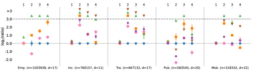
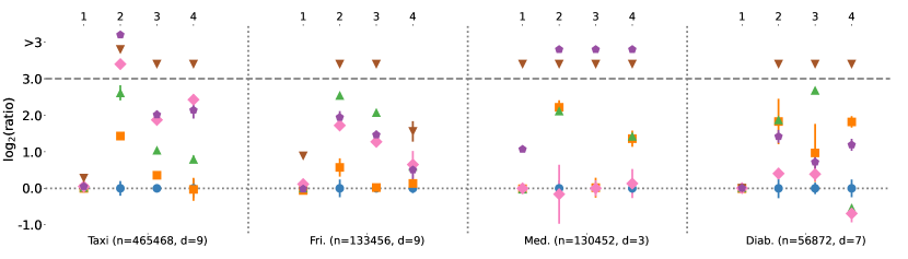
Figure 1: Comparison of PrivPGD with all $2$-Way marginals against state-of-the-art methods based on metrics from Section 4.1: 1) downstream error, 2) covariance error, 3) count. queries error, and 4) thresh. queries error, across 9 tabular datasets. For each method, we plot the $\log_{2}$ ratio of the errors, using PrivPGD’s average error as the denominator, and report the mean and standard deviation over 5 runs. We cut at a log ratio of $y=3$ (dashed line) and list all methods exceeding this threshold above this line in order. We set $\epsilon=2.5$ and $\delta=10^{-5}$.

4.3 Comparison with baselines

We now present how the performance of PrivPGD compares against the state-of-the-art algorithms for DP data synthesis. Figure 1 illustrates the relative performance of PrivPGD compared to other methods, using metrics from Section 4.1. PrivPGD consistently ranks as either the best or the second-best in most metrics and datasets, with a few exceptions such as the covariance error in the ACS Public Coverage dataset.

Comparison with PGM

PrivPGD systematically outperforms both variants of PGM, which are the state-of-the-art for marginal-based tabular data synthesis, often by a significant margin. Specifically, it is better than PGM+MST in covariance and query errors across datasets, except for thresholding query errors in the Diabetes dataset, and performs at least as well as PGM+AIM, usually surpassing it, with the notable exception of thresholding query errors in the ACS Mobility dataset. For downstream tasks, PrivPGD performs comparably to PGM+AIM and consistently better than PGM+MST.

Comparison with query-based algorithms

Furthermore, PrivPGD is also the preferred method in most scenarios when compared to query-based approaches, especially against GEM and RAP. While Private GSD provides competitive performance and occasionally surpasses PrivPGD – for instance, in the ACS Public Coverage dataset – PrivPGD usually emerges as the best-performing method. On many datasets it significantly outperforms Private GSD in all metrics, as exemplified by the Taxi, Black Friday, and ACS Traveltime datasets.

$\text{SW}_{1}$ and TV distance

Finally, Figure 2 illustrates a noticeable performance gap between PrivPGD and other methods when comparing the average sliced Wasserstein distance and the total variation distance. PrivPGD effectively minimizes the former, while state-of-the-art methods like PGM primarily target the latter. Our experiments demonstrate the advantage of minimizing a geometry-aware loss function like the sliced Wasserstein distance over the total variation distance.

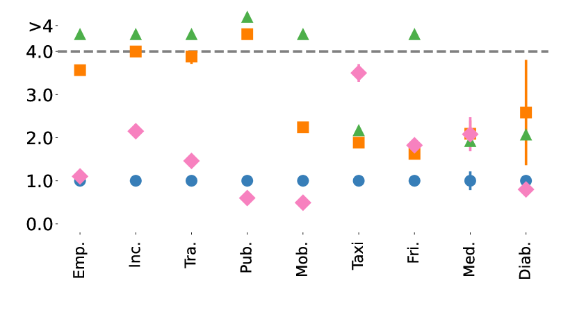
Figure 2: Comparison of average $\text{SW}_{1}$ distance (left) and average TV distance (right) for PrivPGD against state-of-the-art methods across 9 tabular datasets. Similar to Figure 1, we report the mean and standard deviation (5 runs) of the $\log_{2}$ ratio of errors. We set $\epsilon=2.5$ and $\delta=10^{-5}$.

4.4 Enforcing additional domain-specific constraints

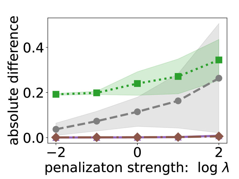
(a) ACS Income

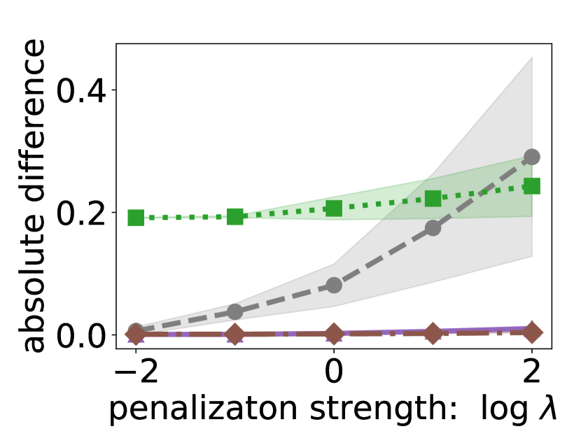
(b) ACS Employment

Figure 3: The absolute error of the domain-specific query (larger is better), the downstream classification error (smaller is better), and the absolute error over counting and thresholding queries (smaller is better), i.e., only the numerator in  Equation 9, as a function of the log regularization strength $\lambda$. We plot the curves for (a) the Income and (b) the Employment dataset.

Section 4.3 shows that PrivPGD constructs a private dataset that successfully preserves the relevant statistics of the original dataset. However, while differential privacy protects individual information, many applications require the protection of specific population-level statistics, i.e., one would like specific statistics from the DP-dataset $D_{\text{DP}}$ to have a large mismatch with statistics from the original dataset $D$. This goal is in contrast to the utility loss that tries to match certain statistics of the original dataset. One example is census data, where it might be desirable to hide religious or sexual orientations at the subpopulation level to prevent potential discriminatory misuse of the data. Another example is the publication of rental and house sale prices, where exposing certain correlations could lead to speculative abuses in specific locales.

We now demonstrate how PrivPGD, while constructing a high-quality dataset, also allows the protection of statistics on a population level. As an example, we consider maximizing the distance of a single linear (non-sparse) thresholding query $\text{thrs}_{\text{Emb}}(Z)=\frac{1}{m}\sum_{i}\mathbbm{1}_{\langle Z_{i},\theta\rangle+b>0}$ defined directly in the embedding space. We approximate this query using a differentiable sigmoid approximation and define $\hat{\mathcal{R}}(Z)=\frac{1}{c+(\triangle(Z))^{2}}$ where $\triangle(Z)$ is the difference to a DP-estimate of the original data. We refer to the Appendix B for implementation details.

We plot in Figure 3 the absolute thresholding error as a function of the regularization strength $\lambda$. While the query is well approximated if no (or only little) regularization is used, we see how increasing the regularization strength increasingly protects these statistics, as the domain-specific counting query on $D_{\text{DP}}$ deviates strongly from the one on the original data $D$. We further plot the downstream error and the absolute errors over random counting and thresholding queries (only the numerator in Equation 9). We observe that, even for larger regularization penalties, these statistics are still preserved, comparable to the unregularized case.

5 Conclusion and future work

We introduced PrivPGD, a novel generation method for marginal-based private data synthesis. Our approach leverages particle gradient descent, combined with techniques from optimal transport, resulting in improved performance in a large number of settings, enhanced scalability for handling numerous marginals and larger datasets, and increased flexibility for accommodating domain-specific constraints compared to existing methods.

Future work could develop regularization penalties that promote an inductive bias in PrivPGD towards more favorable solutions, similar to the maximum entropy bias in PGM. Additionally, exploring the design of domain-specific differentiable constraints and applying our method in practical scenarios presents an exciting avenue for future research.

6 Acknowledgements

KD was supported by the ETH AI Center and the ETH Foundations of Data Science. JA was supported by the ETH AI Center. We thank Aram Alexandre Pooladin and Guillaume Wang for insightful discussions.

Appendix A Extended Experimental Details

Datasets

We use a diverse range of real-world datasets, each with associated classification or regression tasks. Notably, our data sources include the American Community Survey (ACS) and various datasets from [22].

• ACS Income classification dataset (Inc.)  [14]. The dataset focuses on predicting whether an individual earns more than 50,000 dollars annually. It is derived from the ACS PUMS data sample, with specific filters applied: only individuals aged above 16, those who reported working for at least 1 hour weekly in the past year, and those with a reported income exceeding 100 dollars were included. We take the data from California over a 5-year horizon and survey year 2018, with $d=11$ dimension and $n=760,157$ data points.

• ACS Employment classification dataset (Emp.) [14]. The dataset is designed to predict an individual’s employment status. It’s derived from the ACS PUMS data sample but only considers individuals aged between 16 and 90. We take the data from California over a 5-year horizon and survey year 2018, with $d=17$ dimension and $n=1,503,938$ data points.

• ACS Mobility classification dataset (Mob.) [14]. The goal is to determine if an individual retained the same residential address from the previous year using a filtered subset of the ACS PUMS data. This subset exclusively includes individuals aged between 18 and 35. Filtering for this age range heightens the prediction challenge, as over 90% of the broader population typically remains at the same address from one year to the next. We take the data from California over a 5-year horizon and survey year 2018, with $d=22$ dimension and $n=318,332$ data points.

• ACS Traveltime classification dataset (Tra.) [14]. The objective is to predict if an individual’s work commute surpasses 20 minutes using a refined subset of the ACS PUMS data. This subset is limited to those who are employed and are older than 16 years. The 20-minute benchmark was selected based on its status as the median travel time to work for the US population in the 2018 ACS PUMS data release. We take the data from California over a 5-year horizon and survey year 2018, with $d=17$ dimension and $n=667,132$ data points.

• ACS Public Coverage classification dataset (Pub.) [14]. The task is to predict if an individual is enrolled in public health insurance using a specific subset of the ACS PUMS data. This subset is narrowed down to individuals younger than 65 and with an income below 30,000 dollars. By focusing on this group, the prediction centers on low-income individuals who don’t qualify for Medicare. We take the data from California over a 5-year horizon and survey year 2018, with $d=20$ dimension and $n=583,545$ data points.

• Medical charges regression dataset (Med.) [22]. The dataset from the tabular benchmark, part of the “regression on numerical features” benchmark, details inpatient discharges under the Medicare fee-for-service scheme. Known as the Inpatient Utilization and Payment Public Use File (Inpatient PUF), it provides insights into utilization, total and Medicare-specific payments, and hospital-specific charges. The dataset encompasses data from over 3,000 U.S. hospitals under the Medicare Inpatient Prospective Payment System (IPPS) framework. Organized by hospitals and the Medicare Severity Diagnosis Related Group (MS-DRG), this dataset spans from Fiscal Year 2011 to 2016. In total, it contains $n=130,452$ data point with $d=3$ features.

• Black Friday regression dataset (Fri.) [22]. This dataset contains purchases from $n=133,456$ buyers on black Friday. Each point is described by $d=9$ features, including gender, age, occupation and marital status.

• NYC Taxi Green December 2016 regression dataset (Taxi) [22]. The dataset, utilized in the “regression on numerical features” benchmark from the tabular data benchmark, originates from the New York City Taxi and Limousine Commission’s (TLC) trip records for the green line in December 2016. In this processed version, string datetime details have been converted to numeric columns. The goal is to predict the “tip amount”. Records exclusively from credit card payments were retained. The dataset contains $n=465,468$ points with $d=9$ features.

• Diabetes 130-US dataset classification dataset (Diab.) [39]. The dataset encapsulates a decade (1999-2008) of $n=56,872$ clinical observations from 130 US hospitals and integrated delivery systems, comprising over $d=7$ features denoting patient and hospital results. The data was curated based on specific criteria: the record must be of an inpatient hospital admission, be associated with a diabetes diagnosis, have a stay duration ranging from 1 to 14 days, include laboratory tests, and involve medication administration.

Appendix B Additional Details for Section 4.4

We now give additional descriptions for the experiments in Section 4.4. We approximate the thresholding function $\text{thrs}_{\text{Emb}}(Z)=\frac{1}{m}\sum_{i}\mathbbm{1}_{\langle Z_{i},\theta\rangle+b>0}$ using the smooth sigmoid approximation $\text{s-thrsh}_{\text{Emb}}(Z)=\frac{1}{m}\sum_{i}\left(1+\exp(-\sigma(\langle\theta,Z_{i}\rangle-b))\right)^{-1}$ with $\sigma=5.0$. We then split the privacy budget into two parts; the first part $\epsilon=0.5$ and $\delta=2\times 10^{-6}$ is used for obtaining a DP estimate of $\text{s-thrsh}_{\text{Emb}}(\text{Emb}(D))$ using the Gaussian mechanim, which we denote by $\widehat{\text{s-thrsh}}_{\text{Emb}}$. Moreover, we use the remaining privacy budget $\epsilon=2.0$ and $\delta=8\times 10^{-6}$ to privatize all $2$-Way marginals using the Gaussian mechanism as in Algorithm 1. As a result, using the simple composition theorem (see e.g., [17]), the overall algorithm is then DP for $\epsilon=2.5$ and $\delta=10^{-5}$.

Finally, we generate the differentially private dataset $D_{\text{DP}}$ by running Algorithm 3 with all privatized 2-Way marginals as inputs as well as the DP regularization loss

$$\hat{\mathcal{R}}(Z)=\frac{0.01}{0.0001+(\text{s-thrsh}_{\text{Emb}}(Z)-\widehat{\text{s-thrsh}}_{\text{Emb}})^{2}}.$$ (12)

and regularization strength $\lambda$ reaching from $10^{-2}$ to $10$, as depicted in Figure 3.

Appendix C Extended Results for Section 4.3

We replicate Figure 1 with $\epsilon=1.0$ (see Figure 4) and $\epsilon=0.2$ (see Figure 5). At smaller values of $\epsilon$, PrivPGD is more frequently outperformed by PGM, especially in combination with AIM, and also with MST at $\epsilon=0.2$, as well as more often by Private GSD. PGM-based methods benefit from a strong inductive bias towards maximum entropy solutions, which becomes particularly advantageous when noise levels are high. Nevertheless, PrivPGD still maintains highly competitive performance, especially in larger datasets and with fewer features. A similar trend is observed in the total variation and Wasserstein distance, as shown in Figures 6 and 7. These results underscore that PrivPGD’s performance edge diminishes as $\epsilon$ decreases.

Finally, Tables 1 to 6 provide the detailed metrics for all our results.

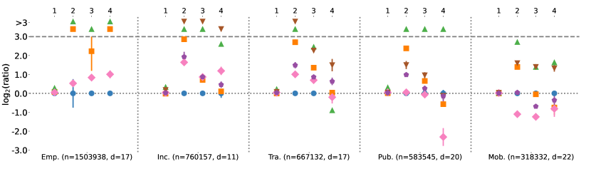
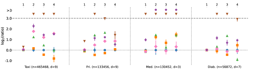
Figure 4: Comparison of PrivPGD with all $2$-way marginals against state-of-the-art methods based on metrics from Section 4.1: 1) downstream error, 2) covariance error, 3) count. queries error, and 4) thresh. queries error, across 9 tabular datasets. For each method, we plot the $\log_{2}$ ratio of the errors, using PrivPGD’s average error as the denominator, and report the mean and standard deviation over 5 runs. We cut at a log ratio of $y=3$ (dashed line) and list all methods exceeding this threshold above this line in order. We set $\epsilon=1.0$ and $\delta=10^{-5}$.

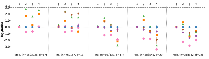
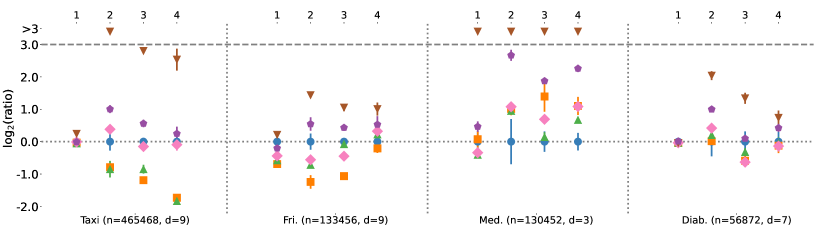
Figure 5: Comparison of PrivPGD with all $2$-way marginals against state-of-the-art methods based on metrics from Section 4.1: 1) downstream error, 2) covariance error, 3) count. queries error, and 4) thresh. queries error, across 9 tabular datasets. For each method, we plot the $\log_{2}$ ratio of the errors, using PrivPGD’s average error as the denominator, and report the mean and standard deviation over 5 runs. We cut at a log ratio of $y=3$ (dashed line) and list all methods exceeding this threshold above this line in order. We set $\epsilon=0.2$ and $\delta=10^{-5}$.

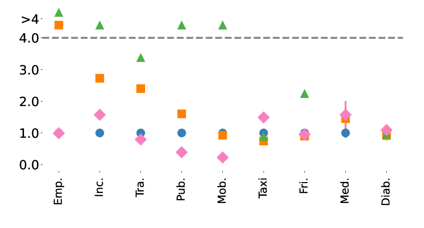
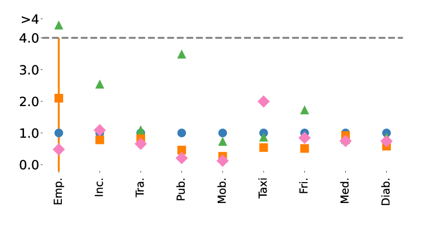
Figure 6: Comparison of average $\text{SW}_{1}$ distance (left) and average TV distance (right) for PrivPGD against state-of-the-art methods across 9 tabular datasets. Similar to Figure 1, we report the mean and standard deviation (5 runs) of the $\log_{2}$ ratio of errors. We set $\epsilon=1.0$ and $\delta=10^{-5}$.

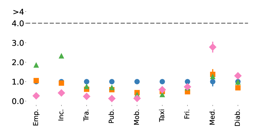
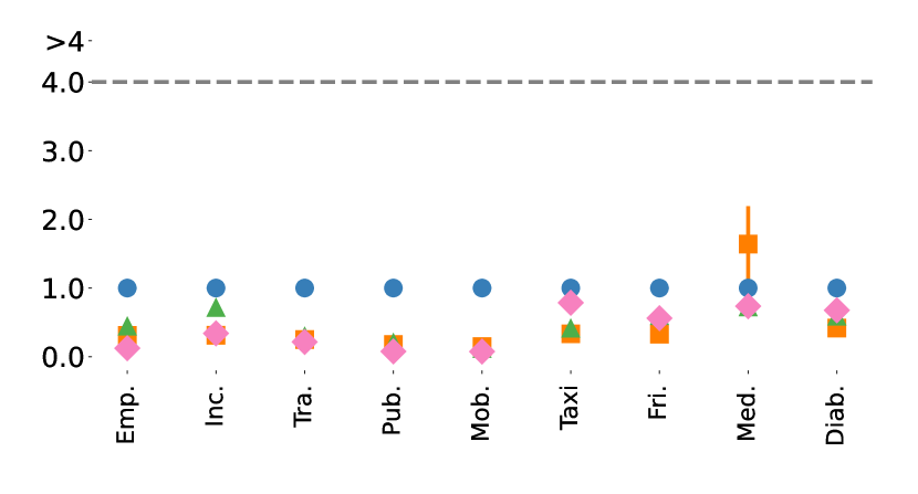
Figure 7: Comparison of average $\text{SW}_{1}$ distance (left) and average TV distance (right) for PrivPGD against state-of-the-art methods across 9 tabular datasets. Similar to Figure 1, we report the mean and standard deviation (5 runs) of the $\log_{2}$ ratio of errors. We set $\epsilon=0.2$ and $\delta=10^{-5}$.

dataset	inference	downstream	covariance	counting query	thresholding query	$\text{SW}_{1}$ distance	TV distance
Emp.	PrivPGD	0.19/0.19	0.02	0.00087	0.00043	0.00054	0.021
	PGM+AIM	0.19/0.19	0.04	0.0025	0.0026	0.0019	0.026
	PGM+MST	0.33/0.19	0.27	0.012	0.0075	0.0087	0.1
	Private GSD	0.2/0.19	0.0083	0.0013	0.00073	0.00059	0.013
Inc.	PrivPGD	0.19/0.19	0.001	0.00078	0.00031	0.00043	0.028
	PGM+AIM	0.19/0.19	0.014	0.0017	0.00034	0.0017	0.034
	PGM+MST	0.24/0.19	0.051	0.0077	0.0024	0.0054	0.11
	Private GSD	0.2/0.19	0.0049	0.0017	0.00083	0.00093	0.045
	GEM	0.22/0.19	0.047	0.01	0.0038	0.0099	0.17
	RAP	0.2/0.19	0.0078	0.0017	0.00056	0.0011	0.037
Tra.	PrivPGD	0.37/0.34	0.0026	0.00065	0.00014	0.00049	0.027
	PGM+AIM	0.37/0.34	0.037	0.0023	0.00031	0.0019	0.035
	PGM+MST	0.46/0.34	0.091	0.0058	0.00032	0.0038	0.061
	Private GSD	0.38/0.34	0.011	0.0017	0.00037	0.00072	0.033
	GEM	0.4/0.34	0.048	0.0052	0.0011	0.0041	0.076
	RAP	0.38/0.34	0.015	0.0019	0.00047	0.0014	0.036
Pub.	PrivPGD	0.28/0.27	0.06	0.00097	0.00033	0.00094	0.037
	PGM+AIM	0.32/0.27	0.1	0.0051	0.0012	0.0042	0.048
	PGM+MST	0.35/0.27	0.41	0.01	0.00074	0.0088	0.092
	Private GSD	0.3/0.27	0.012	0.0016	0.00015	0.00057	0.013
	GEM	0.29/0.27	0.035	0.0031	0.00042	0.0019	0.029
	RAP	0.29/0.27	0.02	0.0015	0.00054	0.0012	0.02
Mob.	PrivPGD	0.23/0.22	0.0091	0.0014	0.00051	0.0011	0.056
	PGM+AIM	0.23/0.22	0.05	0.0029	0.00036	0.0025	0.035
	PGM+MST	0.24/0.22	0.29	0.0088	0.005	0.0095	0.096
	Private GSD	0.24/0.22	0.0092	0.0013	0.00068	0.00055	0.015
	GEM	0.24/0.22	0.063	0.0074	0.0022	0.006	0.082
	RAP	0.23/0.22	0.016	0.0014	0.00066	0.0013	0.022

Table 1: The mean of the errors from Section 4.1 averaged over 5 runs. For the downstream error, we additionally show the test error when training on the original private dataset. We choose $\epsilon=2.5$ and $\delta=10^{-5}$.

dataset	inference	downstream	covariance	counting query	thresholding query	$\text{SW}_{1}$ distance	TV distance
Taxi	PrivPGD	2.3/2.2	0.00048	0.00051	0.00011	0.00027	0.02
	PGM+AIM	2.3/2.2	0.0013	0.00066	0.00011	0.0005	0.016
	PGM+MST	2.3/2.2	0.0029	0.0011	0.0002	0.00058	0.028
	Private GSD	2.3/2.2	0.004	0.0019	0.00061	0.00093	0.064
	GEM	2.7/2.2	0.079	0.016	0.0037	0.018	0.36
	RAP	2.3/2.2	0.0065	0.0021	0.0005	0.0013	0.078
Fri.	PrivPGD	1.5/1.4	0.00097	0.00064	0.00053	0.00033	0.015
	PGM+AIM	1.5/1.4	0.0014	0.00064	0.00058	0.00054	0.011
	PGM+MST	1.5/1.4	0.0057	0.0027	0.0008	0.0014	0.047
	Private GSD	1.7/1.4	0.0032	0.0015	0.00083	0.0006	0.021
	GEM	2.8/1.4	0.031	0.0066	0.0016	0.009	0.16
	RAP	1.5/1.4	0.0038	0.0018	0.00075	0.0011	0.034
Med.	PrivPGD	2.2/2.1	0.00014	0.0012	0.00013	0.00036	0.023
	PGM+AIM	2.1/2.1	0.00066	0.0012	0.00034	0.00076	0.013
	PGM+MST	2.1/2.1	0.00061	0.0012	0.00035	0.0007	0.017
	Private GSD	2.2/2.1	0.00013	0.0012	0.00014	0.00076	0.02
	GEM	75/2.1	0.11	0.1	0.054	0.22	1.4
	RAP	4.5/2.1	0.0048	0.013	0.0023	0.007	0.062
Diab.	PrivPGD	0.4/0.4	0.0013	0.0013	0.00042	0.00084	0.028
	PGM+AIM	0.4/0.4	0.0045	0.0025	0.0015	0.0022	0.028
	PGM+MST	0.41/0.4	0.0047	0.0083	0.00029	0.0017	0.045
	Private GSD	0.41/0.4	0.0017	0.0017	0.00026	0.00067	0.026
	GEM	0.41/0.4	0.042	0.032	0.0084	0.032	0.23
	RAP	0.41/0.4	0.0034	0.0021	0.00097	0.0025	0.041

Table 2: The mean of the errors from Section 4.1 averaged over 5 runs. For the downstream error, we additionally show the test error when training on the original private dataset. We choose $\epsilon=2.5$ and $\delta=10^{-5}$.

dataset	inference	downstream	covariance	counting query	thresholding query	$\text{SW}_{1}$ distance	TV distance
Emp.	PrivPGD	0.19/0.19	0.0056	0.00077	0.00038	0.0006	0.027
	PGM+AIM	0.2/0.19	0.063	0.0036	0.004	0.0042	0.057
	PGM+MST	0.23/0.19	0.48	0.098	0.081	0.14	0.7
	Private GSD	0.2/0.19	0.008	0.0014	0.00076	0.00059	0.013
Inc.	PrivPGD	0.19/0.19	0.0019	0.00092	0.00039	0.0006	0.042
	PGM+AIM	0.19/0.19	0.014	0.0015	0.00042	0.0016	0.033
	PGM+MST	0.24/0.19	0.052	0.0077	0.0024	0.0054	0.11
	Private GSD	0.2/0.19	0.0061	0.0017	0.00089	0.00095	0.046
	GEM	0.22/0.19	0.047	0.01	0.0037	0.0098	0.16
	RAP	0.19/0.19	0.0074	0.0017	0.00054	0.001	0.041
Tra.	PrivPGD	0.37/0.34	0.0055	0.0011	0.00032	0.00091	0.05
	PGM+AIM	0.37/0.34	0.036	0.0027	0.00033	0.0022	0.042
	PGM+MST	0.44/0.34	0.073	0.0058	0.00017	0.0031	0.055
	Private GSD	0.38/0.34	0.011	0.0017	0.00028	0.00072	0.033
	GEM	0.4/0.34	0.048	0.0051	0.00091	0.004	0.074
	RAP	0.38/0.34	0.016	0.0019	0.0005	0.0016	0.041
Pub.	PrivPGD	0.28/0.27	0.011	0.0015	0.00061	0.0014	0.061
	PGM+AIM	0.28/0.27	0.058	0.0024	0.00041	0.0023	0.028
	PGM+MST	0.35/0.27	0.29	0.024	0.0092	0.04	0.21
	Private GSD	0.29/0.27	0.012	0.0014	0.00012	0.00055	0.013
	GEM	0.29/0.27	0.031	0.0029	0.00056	0.0017	0.025
	RAP	0.29/0.27	0.022	0.0018	0.00055	0.0014	0.023
Mob.	PrivPGD	0.23/0.22	0.021	0.0029	0.00085	0.0026	0.13
	PGM+AIM	0.23/0.22	0.054	0.0028	0.00051	0.0024	0.034
	PGM+MST	0.24/0.22	0.13	0.0077	0.0027	0.013	0.093
	Private GSD	0.24/0.22	0.0096	0.0012	0.00049	0.0006	0.016
	GEM	0.24/0.22	0.062	0.0077	0.0021	0.0062	0.083
	RAP	0.23/0.22	0.021	0.0018	0.00066	0.0017	0.031

Table 3: The mean of the errors from Section 4.1 averaged over 5 runs. For the downstream error, we additionally show the test error when training on the original private dataset. We choose $\epsilon=1.0$ and $\delta=10^{-5}$.

dataset	inference	downstream	covariance	counting query	thresholding query	$\text{SW}_{1}$ distance	TV distance
Taxi	PrivPGD	2.3/2.2	0.0013	0.00077	0.00018	0.00062	0.033
	PGM+AIM	2.3/2.2	0.0014	0.00057	0.00011	0.00046	0.018
	PGM+MST	2.3/2.2	0.003	0.0011	0.00018	0.00055	0.029
	Private GSD	2.4/2.2	0.0043	0.0018	0.00055	0.00092	0.066
	GEM	2.8/2.2	0.081	0.017	0.0045	0.021	0.36
	RAP	2.3/2.2	0.0061	0.0021	0.00052	0.0014	0.08
Fri.	PrivPGD	1.6/1.4	0.0022	0.00086	0.00053	0.00068	0.028
	PGM+AIM	1.5/1.4	0.0016	0.00071	0.00056	0.00061	0.014
	PGM+MST	1.5/1.4	0.0058	0.0027	0.00081	0.0015	0.049
	Private GSD	1.6/1.4	0.0031	0.0015	0.00096	0.00065	0.024
	GEM	2.8/1.4	0.031	0.0068	0.0014	0.0092	0.16
	RAP	1.6/1.4	0.0048	0.002	0.00078	0.0016	0.046
Med.	PrivPGD	2.4/2.1	0.00032	0.0015	0.00019	0.00061	0.03
	PGM+AIM	2.3/2.1	0.00076	0.0024	0.00053	0.00088	0.027
	PGM+MST	2.1/2.1	0.00088	0.0018	0.00051	0.001	0.023
	Private GSD	2.2/2.1	0.00041	0.0014	0.00024	0.00095	0.022
	GEM	75/2.1	0.11	0.1	0.054	0.22	1.4
	RAP	4.7/2.1	0.0051	0.013	0.0024	0.007	0.066
Diab.	PrivPGD	0.4/0.4	0.0033	0.0026	0.001	0.002	0.052
	PGM+AIM	0.4/0.4	0.0031	0.0019	0.0014	0.0019	0.03
	PGM+MST	0.41/0.4	0.0042	0.0067	0.00056	0.0019	0.045
	Private GSD	0.41/0.4	0.0036	0.0024	0.00096	0.0022	0.039
	GEM	0.41/0.4	0.04	0.031	0.0078	0.03	0.22
	RAP	0.41/0.4	0.0073	0.0043	0.002	0.0054	0.071

Table 4: The mean of the errors from Section 4.1 averaged over 5 runs. For the downstream error, we additionally show the test error when training on the original private dataset. We choose $\epsilon=1.0$ and $\delta=10^{-5}$.

dataset	inference	downstream	covariance	counting query	thresholding query	$\text{SW}_{1}$ distance	TV distance
Emp.	PrivPGD	0.19/0.19	0.015	0.0022	0.00078	0.0023	0.11
	PGM+AIM	0.19/0.19	0.049	0.0027	0.0031	0.0024	0.035
	PGM+MST	0.23/0.19	0.1	0.0067	0.0047	0.0043	0.05
	Private GSD	0.2/0.19	0.0088	0.0014	0.00083	0.00063	0.014
Inc.	PrivPGD	0.19/0.19	0.0098	0.0027	0.00086	0.0024	0.15
	PGM+AIM	0.19/0.19	0.019	0.0025	0.00053	0.0022	0.048
	PGM+MST	0.24/0.19	0.052	0.0077	0.0024	0.0056	0.11
	Private GSD	0.2/0.19	0.0058	0.0018	0.0008	0.001	0.052
	GEM	0.22/0.19	0.046	0.0099	0.0035	0.0096	0.16
	RAP	0.2/0.19	0.011	0.0024	0.001	0.0019	0.072
Tra.	PrivPGD	0.38/0.34	0.027	0.0043	0.0012	0.004	0.19
	PGM+AIM	0.37/0.34	0.05	0.0028	0.00027	0.0024	0.048
	PGM+MST	0.44/0.34	0.07	0.0058	0.00018	0.003	0.057
	Private GSD	0.38/0.34	0.012	0.0019	0.00033	0.00097	0.041
	GEM	0.4/0.34	0.048	0.0051	0.00093	0.004	0.073
	RAP	0.39/0.34	0.026	0.003	0.00093	0.0033	0.074
Pub.	PrivPGD	0.29/0.27	0.048	0.0058	0.0021	0.0064	0.24
	PGM+AIM	0.29/0.27	0.1	0.0039	0.00093	0.0037	0.043
	PGM+MST	0.31/0.27	0.16	0.0062	0.00031	0.0045	0.05
	Private GSD	0.29/0.27	0.014	0.0017	0.0002	0.00085	0.019
	GEM	0.29/0.27	0.044	0.0039	0.00053	0.0025	0.035
	RAP	0.29/0.27	0.037	0.0033	0.0013	0.003	0.049
Mob.	PrivPGD	0.24/0.22	0.085	0.014	0.003	0.011	0.46
	PGM+AIM	0.23/0.22	0.14	0.0052	0.0019	0.0049	0.068
	PGM+MST	0.24/0.22	0.12	0.006	0.0019	0.0037	0.054
	Private GSD	0.24/0.22	0.018	0.0019	0.00076	0.0016	0.035
	GEM	0.24/0.22	0.062	0.0076	0.0018	0.0058	0.078
	RAP	0.24/0.22	0.048	0.0043	0.0012	0.0048	0.08

Table 5: The mean of the errors from Section 4.1 averaged over 5 runs. For the downstream error, we additionally show the test error when training on the original private dataset. We choose $\epsilon=0.2$ and $\delta=10^{-5}$.

dataset	inference	downstream	covariance	counting query	thresholding query	$\text{SW}_{1}$ distance	TV distance
Taxi	PrivPGD	2.4/2.2	0.0055	0.0025	0.00072	0.0026	0.11
	PGM+AIM	2.3/2.2	0.0032	0.0011	0.00022	0.0013	0.037
	PGM+MST	2.3/2.2	0.003	0.0014	0.0002	0.00087	0.046
	Private GSD	2.4/2.2	0.0071	0.0022	0.00068	0.0015	0.087
	GEM	2.8/2.2	0.082	0.017	0.0042	0.02	0.36
	RAP	2.4/2.2	0.011	0.0036	0.00086	0.0036	0.17
Fri.	PrivPGD	2.5/1.4	0.011	0.0031	0.00071	0.0031	0.11
	PGM+AIM	1.5/1.4	0.0048	0.0015	0.00061	0.0015	0.036
	PGM+MST	1.6/1.4	0.0069	0.003	0.00082	0.0021	0.065
	Private GSD	1.8/1.4	0.0077	0.0023	0.00088	0.0023	0.061
	GEM	2.8/1.4	0.031	0.0065	0.0014	0.0083	0.15
	RAP	2.1/1.4	0.017	0.0042	0.001	0.0055	0.12
Med.	PrivPGD	3/2.1	0.0013	0.0048	0.00082	0.0024	0.076
	PGM+AIM	3.1/2.1	0.0027	0.013	0.0018	0.0033	0.12
	PGM+MST	2.2/2.1	0.0026	0.0053	0.0013	0.0031	0.055
	Private GSD	2.3/2.1	0.0028	0.0078	0.0017	0.0067	0.056
	GEM	76/2.1	0.11	0.1	0.054	0.21	1.4
	RAP	4.1/2.1	0.0084	0.018	0.0039	0.01	0.1
Diab.	PrivPGD	0.42/0.4	0.01	0.013	0.0045	0.0082	0.17
	PGM+AIM	0.41/0.4	0.011	0.0085	0.0042	0.0056	0.071
	PGM+MST	0.41/0.4	0.012	0.01	0.0044	0.008	0.1
	Private GSD	0.41/0.4	0.014	0.0083	0.0041	0.011	0.12
	GEM	0.41/0.4	0.043	0.033	0.0076	0.032	0.23
	RAP	0.42/0.4	0.021	0.014	0.0061	0.018	0.19

Table 6: The mean of the errors from Section 4.1 averaged over 5 runs. For the downstream error, we additionally show the test error when training on the original private dataset. We choose $\epsilon=0.2$ and $\delta=10^{-5}$.

References

- Abowd [2018] John M Abowd. The US Census Bureau adopts differential privacy. In Proceedings of the 24th ACM SIGKDD international conference on knowledge discovery & data mining, pages 2867–2867, 2018.
- Aktay et al. [2020] Ahmet Aktay, Shailesh Bavadekar, Gwen Cossoul, John Davis, Damien Desfontaines, Alex Fabrikant, Evgeniy Gabrilovich, Krishna Gadepalli, Bryant Gipson, Miguel Guevara, et al. Google COVID-19 community mobility reports: anonymization process description (version 1.1). arXiv preprint arXiv:2004.04145, 2020.
- Asghar et al. [2019] Hassan Jameel Asghar, Ming Ding, Thierry Rakotoarivelo, Sirine Mrabet, and Mohamed Ali Kaafar. Differentially private release of high-dimensional datasets using the Gaussian copula. arXiv preprint arXiv:1902.01499, 2019.
- Aydore et al. [2021] Sergul Aydore, William Brown, Michael Kearns, Krishnaram Kenthapadi, Luca Melis, Aaron Roth, and Ankit A Siva. Differentially private query release through adaptive projection. In Proceedings of the International Conference on Machine Learning, pages 457–467, 2021.
- Boedihardjo et al. [2022] March Boedihardjo, Thomas Strohmer, and Roman Vershynin. Private measures, random walks, and synthetic data. arXiv preprint arXiv:2204.09167, 2022.
- Bonneel et al. [2015] Nicolas Bonneel, Julien Rabin, Gabriel Peyré, and Hanspeter Pfister. Sliced and Radon Wasserstein barycenters of measures. Journal of Mathematical Imaging and Vision, 51:22–45, 2015.
- Buitinck et al. [2013] Lars Buitinck, Gilles Louppe, Mathieu Blondel, Fabian Pedregosa, Andreas Mueller, Olivier Grisel, Vlad Niculae, Peter Prettenhofer, Alexandre Gramfort, Jaques Grobler, Robert Layton, Jake VanderPlas, Arnaud Joly, Brian Holt, and Gaël Varoquaux. API design for machine learning software: experiences from the scikit-learn project. In ECML PKDD Workshop: Languages for Data Mining and Machine Learning, pages 108–122, 2013.
- Cai et al. [2021] Kuntai Cai, Xiaoyu Lei, Jianxin Wei, and Xiaokui Xiao. Data synthesis via differentially private Markov random fields. Proceedings of the VLDB Endowment, 14(11):2190–2202, 2021.
- Cao et al. [2021] Tianshi Cao, Alex Bie, Arash Vahdat, Sanja Fidler, and Karsten Kreis. Don’t generate me: Training differentially private generative models with sinkhorn divergence. Advances in Neural Information Processing Systems, 34:12480–12492, 2021.
- Dankar and El Emam [2012] Fida Kamal Dankar and Khaled El Emam. The application of differential privacy to health data. In Proceedings of the 2012 Joint EDBT/ICDT Workshops, pages 158–166, 2012.
- Deshpande et al. [2018] Ishan Deshpande, Ziyu Zhang, and Alexander G Schwing. Generative modeling using the sliced Wasserstein distance. In Proceedings of the IEEE conference on computer vision and pattern recognition, pages 3483–3491, 2018.
- Deshpande et al. [2019] Ishan Deshpande, Yuan-Ting Hu, Ruoyu Sun, Ayis Pyrros, Nasir Siddiqui, Sanmi Koyejo, Zhizhen Zhao, David Forsyth, and Alexander G Schwing. Max-sliced Wasserstein distance and its use for GANs. In Proceedings of the IEEE/CVF Conference on Computer Vision and Pattern Recognition, pages 10648–10656, 2019.
- DiMaggio [2013] Charles DiMaggio. SAS for epidemiologists: applications and methods. Springer, 2013.
- Ding et al. [2021] Frances Ding, Moritz Hardt, John Miller, and Ludwig Schmidt. Retiring Adult: New datasets for fair machine learning. Advances in Neural Information Processing Systems, 34, 2021.
- Donhauser et al. [2023] Konstantin Donhauser, Johan Lokna, Amartya Sanyal, March Boedihardjo, Robert Hönig, and Fanny Yang. Sample-efficient private data release for lipschitz functions under sparsity assumptions. arXiv preprint arXiv:2302.09680, 2023.
- Dwork [2006] Cynthia Dwork. Differential privacy. In Automata, Languages and Programming, pages 1–12, 2006.
- Dwork and Nissim [2004] Cynthia Dwork and Kobbi Nissim. Privacy-preserving datamining on vertically partitioned databases. In Advances in Cryptology–CRYPTO 2004: International Cryptology Conference, pages 528–544, 2004.
- Dwork and Roth [2014] Cynthia Dwork and Aaron Roth. The algorithmic foundations of differential privacy. Foundations and Trends in Theoretical Computer Science, 9(3–4):211–407, 2014.
- El Emam [2011] Khaled El Emam. The case for de-identifying personal health information. SSRN Electronic Journal, 2011.
- Gaboardi et al. [2014] Marco Gaboardi, Emilio Jesus Gallego Arias, Justin Hsu, Aaron Roth, and Zhiwei Steven Wu. Dual Query: Practical private query release for high dimensional data. In Proceedings of the International Conference on Machine Learning, volume 32, pages 1170–1178, 22–24 Jun 2014.
- Gambs et al. [2021] Sébastien Gambs, Frédéric Ladouceur, Antoine Laurent, and Alexandre Roy-Gaumond. Growing synthetic data through differentially-private vine copulas. Proc. Priv. Enhancing Technol., 2021(3):122–141, 2021.
- Grinsztajn et al. [2022] Léo Grinsztajn, Edouard Oyallon, and Gaël Varoquaux. Why do tree-based models still outperform deep learning on typical tabular data? Advances in Neural Information Processing Systems, 35:507–520, 2022.
- Hardt et al. [2012] Moritz Hardt, Katrina Ligett, and Frank Mcsherry. A simple and practical algorithm for differentially private data release. In Advances in Neural Information Processing Systems, volume 25, 2012.
- Hu et al. [2024] Yuzheng Hu, Fan Wu, Qinbin Li, Yunhui Long, Gonzalo Munilla Garrido, Chang Ge, Bolin Ding, David Forsyth, Bo Li, and Dawn Song. SoK: Privacy-preserving data synthesis. In 2024 IEEE Symposium on Security and Privacy (SP). IEEE Computer Society, may 2024. doi: 10.1109/SP54263.2024.00002.
- Johnson et al. [2018] Noah Johnson, Joseph P Near, and Dawn Song. Towards practical differential privacy for SQL queries. Proceedings of the VLDB Endowment, 11(5):526–539, 2018.
- Jordon et al. [2019] James Jordon, Jinsung Yoon, and Mihaela Van Der Schaar. PATE-GAN: Generating synthetic data with differential privacy guarantees. In Proceedings of the International conference on learning representations, 2019.
- Kenthapadi et al. [2012] Krishnaram Kenthapadi, Aleksandra Korolova, Ilya Mironov, and Nina Mishra. Privacy via the Johnson-Lindenstrauss transform. J. Priv. Confidentiality, 5, 2012.
- Kolouri et al. [2018] Soheil Kolouri, Gustavo K Rohde, and Heiko Hoffmann. Sliced Wasserstein distance for learning gaussian mixture models. In Proceedings of the IEEE Conference on Computer Vision and Pattern Recognition, pages 3427–3436, 2018.
- Li et al. [2014] Haoran Li, Li Xiong, and Xiaoqian Jiang. Differentially private synthesization of multi-dimensional data using copula functions. In Advances in database technology: proceedings. International conference on extending database technology, volume 2014, page 475. NIH Public Access, 2014.
- Li et al. [2021] Ninghui Li, Zhikun Zhang, and Tianhao Wang. DPSyn: Experiences in the NIST differential privacy data synthesis challenges. Journal of Privacy and Confidentiality, 11, 2021.
- Liu et al. [2021a] Terrance Liu, Giuseppe Vietri, Thomas Steinke, Jonathan Ullman, and Steven Wu. Leveraging public data for practical private query release. In Proceedings of the International Conference on Machine Learning, pages 6968–6977, 2021a.
- Liu et al. [2021b] Terrance Liu, Giuseppe Vietri, and Steven Z Wu. Iterative methods for private synthetic data: Unifying framework and new methods. Advances in Neural Information Processing Systems, 34:690–702, 2021b.
- Liu et al. [2023] Terrance Liu, Jingwu Tang, Giuseppe Vietri, and Steven Wu. Generating private synthetic data with genetic algorithms. In Proceedings of the 40th International Conference on Machine Learning, volume 202 of Proceedings of Machine Learning Research, pages 22009–22027, 23–29 Jul 2023.
- McKenna et al. [2019] Ryan McKenna, Daniel Sheldon, and Gerome Miklau. Graphical-model based estimation and inference for differential privacy. In International Conference on Machine Learning, pages 4435–4444. PMLR, 2019.
- McKenna et al. [2021] Ryan McKenna, Gerome Miklau, and Daniel Sheldon. Winning the NIST contest: A scalable and general approach to differentially private synthetic data. Journal of Privacy and Confidenciality, 2021.
- McKenna et al. [2022] Ryan McKenna, Brett Mullins, Daniel Sheldon, and Gerome Miklau. AIM: An adaptive and iterative mechanism for differentially private synthetic data. Proc. VLDB Endow., 15(11):2599–2612, jul 2022. ISSN 2150-8097. doi: 10.14778/3551793.3551817.
- McSherry and Talwar [2007] Frank McSherry and Kunal Talwar. Mechanism design via differential privacy. In IEEE Symposium on Foundations of Computer Science, pages 94–103, 2007.
- Near and Darais [2022] Joseph Near and David Darais. Differential privacy: Future work & open challenges, 2022. Accessed on 11th October 2023.
- Strack et al. [2014] Beata Strack, Jonathan P DeShazo, Chris Gennings, Juan L Olmo, Sebastian Ventura, Krzysztof J Cios, John N Clore, et al. Impact of HbA1c measurement on hospital readmission rates: analysis of 70,000 clinical database patient records. BioMed research international, 2014, 2014.
- Tao et al. [2021] Yuchao Tao, Ryan McKenna, Michael Hay, Ashwin Machanavajjhala, and Gerome Miklau. Benchmarking differentially private synthetic data generation algorithms. arXiv preprint arXiv:2112.09238, 2021.
- Torkzadehmahani et al. [2019] Reihaneh Torkzadehmahani, Peter Kairouz, and Benedict Paten. DP-CGAN: Differentially private synthetic data and label generation. In Proceedings of the IEEE/CVF Conference on Computer Vision and Pattern Recognition Workshops, 2019.
- Vallender [1974] S. S. Vallender. Calculation of the Wasserstein distance between probability distributions on the line. Theory of Probability & Its Applications, 18(4):784–786, 1974.
- Vero et al. [2023] Mark Vero, Mislav Balunović, and Martin Vechev. Programmable synthetic tabular data generation. arXiv preprint arXiv:2307.03577, 2023.
- Vietri et al. [2020] Giuseppe Vietri, Grace Tian, Mark Bun, Thomas Steinke, and Steven Wu. New oracle-efficient algorithms for private synthetic data release. In Proceedings of the International Conference on Machine Learning, pages 9765–9774, 2020.
- Vietri et al. [2022] Giuseppe Vietri, Cedric Archambeau, Sergul Aydore, William Brown, Michael Kearns, Aaron Roth, Ankit Siva, Shuai Tang, and Steven Z Wu. Private synthetic data for multitask learning and marginal queries. Advances in Neural Information Processing Systems, 35:18282–18295, 2022.
- Wang et al. [2016] Ziteng Wang, Chi Jin, Kai Fan, Jiaqi Zhang, Junliang Huang, Yiqiao Zhong, and Liwei Wang. Differentially private data releasing for smooth queries. The Journal of Machine Learning Research, 17(1):1779–1820, 2016.
- Wu et al. [2019] Jiqing Wu, Zhiwu Huang, Dinesh Acharya, Wen Li, Janine Thoma, Danda Pani Paudel, and Luc Van Gool. Sliced Wasserstein generative models. In Proceedings of the IEEE/CVF Conference on Computer Vision and Pattern Recognition, pages 3713–3722, 2019.
- Xie et al. [2018] Liyang Xie, Kaixiang Lin, Shu Wang, Fei Wang, and Jiayu Zhou. Differentially private generative adversarial network. arXiv preprint arXiv:1802.06739, 2018.
- Xu et al. [2017] Chugui Xu, Ju Ren, Yaoxue Zhang, Zhan Qin, and Kui Ren. DPPro: Differentially private high-dimensional data release via random projection. IEEE Transactions on Information Forensics and Security, 12(12):3081–3093, 2017.
- Zhang et al. [2016] Jun Zhang, Xiaokui Xiao, and Xing Xie. PrivTree: A differentially private algorithm for hierarchical decompositions. In Proceedings of the international conference on management of data, pages 155–170, 2016.
- Zhang et al. [2017] Jun Zhang, Graham Cormode, Cecilia M Procopiuc, Divesh Srivastava, and Xiaokui Xiao. PrivBayes: Private data release via Bayesian networks. ACM Transactions on Database Systems (TODS), 42(4):1–41, 2017.
- Zhang et al. [2021] Zhikun Zhang, Tianhao Wang, Ninghui Li, Jean Honorio, Michael Backes, Shibo He, Jiming Chen, and Yang Zhang. PrivSyn: Differentially private data synthesis. In 30th USENIX Security Symposium (USENIX Security 21), pages 929–946, 2021.