Similarity and Comparison Complexity

Abstract

Some choice options are more difficult to compare than others. This paper develops a theory of what makes a comparison complex, and how comparison complexity generates systematic mistakes in choice. In our model, options are easier to compare when they 1) share similar features, holding fixed their value difference, and 2) are closer to dominance. We show how these two postulates yield tractable measures of comparison complexity in the domains of multiattribute, lottery, and intertemporal choice. Using experimental data on binary choices, we demonstrate that our complexity measures predict choice errors, choice inconsistency, and cognitive uncertainty across all three domains. We then show how canonical anomalies in choice and valuation, such as context effects, preference reversals, and apparent probability weighting and present bias in the valuation of risky and intertemporal prospects, can be understood as responses to comparison complexity.

Keywords: Complexity, multi-attribute choice, choice under risk, intertemporal choice, cognitive uncertainty, experiments

1 Introduction

Some choice options are hard to compare, and this difficulty leads to errors in decision-making. Individuals choose health insurance plans, savings vehicles, and cell phone plans that are in reality financially dominated. Even in settings where objective choice errors cannot be identified, introspection reveals that we often face difficult comparisons: how should one choose between job offers that differ in salary and equity compensation, mortgages with different repayment schedules, or housecats of varying size and temperament? We worry or even agonize over choosing incorrectly in such contexts, and these mistakes not only have private welfare costs for market participants, but may also shape how markets function.

While a growing economic literature on complexity considers what makes choices difficult, most theories of complexity operate at the option level — that is, they tell us what makes a choice option difficult to value (e.g., Enke and Graeber,, 2023; Enke et al.,, 2023; Puri,, 2023; Khaw et al.,, 2021). While this difficulty may shape behavior in certain contexts, people often choose by comparing options directly rather than by producing absolute valuations, and there are important differences between what makes options hard to compare vs. hard to value. For instance, two lotteries may be difficult to value in the sense of having many states, yet easy to compare if one lottery transparently dominates the other.

In this paper, we seek to answer two questions. First, what makes choice options hard to compare? We develop a theory of comparison complexity applicable to the domains of multiattribute, lottery, and intertemporal choice, which formalizes the intuition that options are harder to compare when they require the decision-maker to aggregate trade-offs across option features. We then test our theory using rich experimental data on binary choices across all three domains, and demonstrate its predictive power relative to benchmark models. Second, what are the behavioral consequences of comparison complexity? We embed our theory of comparison complexity into a stochastic choice model in which the decision-maker chooses based on noisy signals of how options compare, the precision of which are governed by our theory of comparison complexity. We use our choice model to shed light on various systematic anomalies in choice and valuation, including context effects, preference reversals, and apparent probability weighting and hyperbolic discounting in the valuation of risky and intertemporal prospects. Through the lens of our model, these phenomena can all be understood as a response to the cognitive difficulty of making comparisons.

Theory of comparison complexity. We develop a theory of comparison complexity, which we formalize as the difficulty of identifying one’s preferred option from a binary menu. We consider a decision-maker who is uncertain about the values of two options $x$ and $y$, and chooses based on a noisy signal of how the values compare. The precision of this signal, $\tau_{xy}$, captures the ease of comparison between $x$ and $y$, and governs the decision-maker’s likelihood of choosing the higher value option. We propose a theory of how $\tau_{xy}$ depends on the features of choice options, applicable to the domains of multiattribute, lottery, and intertemporal choice.

(a) Multiattribute

$\begin{array}[]{ll}x:&\text{\$11/month, \$3.35/GB}\\ x^{\prime}:&\text{\$32/month, \$1.6/GB}\\ y:&\text{\$10.5/month, \$4.45/GB}\end{array}$

(b) Lottery

$\begin{array}[]{ll}x:&\text{\$27 w.p. 25\%, \$3 w.p. 75\%}\\ x^{\prime}:&\text{\$9 for sure}\\ y:&\text{\$20 w.p. 20\%, \$3.2 w.p. 80\%}\\ \end{array}$

(c) Intertemporal

$\begin{array}[]{ll}x:&\text{\$60 in 61 days}\\ x^{\prime}:&\text{\$100 in 3 years}\\ y:&\text{\$40 in 60 days}\end{array}$

Figure 1: Choice Domains. Comparisons between a) phone plans characterized by a monthly and data use fee, b) monetary lotteries, and c) payoff flows. Note that $x\sim x^{\prime}$ for a) a known monthly data usage rate of 12 GB, b) a risk-neutral agent, and c) a monthly discount rate of $\delta=0.95$.

Much previous work argues that complexity arises when decision-makers must aggregate different problem features to reach a conclusion. Our theory is motivated by the simple observation that comparisons involve aggregating trade-offs across option features, and that not all comparisons require the same degree of aggregation. To illustrate, consider the three choice environments in Figure 1. Notice that across these domains, the comparison between $x$ and $y$ is easy — there is little need to make trade-offs across option features to see that $x$ is in fact better than $y$. On the other hand, the comparison between $x^{\prime}$ and $y$ is less obvious, as the DM now must engage with non-trivial trade-offs across different option features: 1a) involves a trade-off between the monthly fee vs. usage fee, 1b) involves trading off a higher maximum payout against a lower payout probability, and 1c) involves a trade-off between payout amount and delay.

Our theory is built on two formal principles that capture this notion of trade-off complexity: similarity and dominance. First, we posit that holding fixed their value difference, options are easier to compare if they are more similar — that is, that the ease of comparison is an increasing transformation $H$ of the value-dissimilarity ratio:

$$\tau_{xy}=H\left(\frac{|U(x)-U(y)|}{d(x,y)}\right),$$

where the numerator contains the value difference between the two options and the denominator is a distance metric measuring their dissimilarity. Intuitively, similar options require less aggregation of trade-offs to compare, as the DM can divert attention from features that are similar across options and so more easily assess their differences. This intuition echoes work in psychology (Tversky and Edward Russo,, 1969) and in economics (Rubinstein,, 1988; He and Natenzon,, 2023) which has stressed the role of similarity in governing the ease of comparison.

Domain	Representation for $\boldsymbol{\tau_{xy}}$	Distance Metric
Multiattribute $U(x)=\sum_{k}\beta_{k}x_{k}$	$\tau_{xy}=H\left(\dfrac{|U(x)-U(y)|}{d_{L1}(x,y)}\right)$	$d_{L1}(x,y)=\displaystyle\sum_{k}|\beta_{k}(x_{k}-y_{k})|$
Lottery $EU(x)=\sum_{w}u(w)f_{x}(w)$	$\tau_{xy}=H\left(\dfrac{|EU(x)-EU(y)|}{d_{CDF}(x,y)}\right)$	$d_{CDF}(x,y)=\displaystyle\int_{0}^{1}|u(F^{-1}_{x}(q))-u(F^{-1}_{y}(q))|\,dq$
Intertemporal $PV(x)=\sum_{t}\delta^{t}x_{t}$	$\tau_{xy}=H\left(\dfrac{|PV(x)-PV(y)|}{d_{CPF}(x,y)}\right)$	$d_{CPF}(x,y)=\ln(1/\delta)\displaystyle\int_{0}^{\infty}|M_{x}(t)-M_{y}(t)|\delta^{t}\,dt$

Table 1: Complexity Measures. $F_{x}^{-1}(q)=\inf\{w\in\mathbb{R}:q\leq F_{x}(w)\}$ denotes the quantile function of a lottery $x$.
$M_{x}(t)=\sum_{t^{\prime}<t}x_{t^{\prime}}$ denotes the cumulative payoff function of a payoff flow $x$.

To pin down the specific dissimilarity measure, we appeal to our second principle: that options are maximally easy to compare in the presence of dominance. Dominance eliminates the need to aggregate trade-offs across features, and to the extent decision-makers find this aggregation difficult, comparisons involving dominance relationships should be more accurate than comparisons that do not. The relevant dominance notions in each of our domains — attribute-wise dominance in multiattribute choice, first-order stochastic dominance in lottery choice, and temporal dominance in intertemporal choice — give rise to the appropriate dissimilarity measure in each domain, summarized in Table 1; for each of these measures, options are maximally easy to compare when they share a dominance relationship.

The postulates of similarity and dominance are not only satisfied by our representations, but also are key in characterizing them; we show that axioms on binary choice behavior corresponding to the postulates of similarity and dominance, in tandem with other easily understood axioms, characterize our representations of $\tau_{xy}$ in each domain.

Tests of complexity measures. Our theory predicts that in binary choice, the prevalence of 1) choice errors, 2) within-individual choice inconsistency, and 3) subjective uncertainty over choices should be decreasing in the value-dissimilarity ratio. Using three experimental datasets on binary choices corresponding to our three domains of interest, we show that the value-dissimilarity ratio is strongly predictive of each of these behavioral indicators of choice complexity. We collect datasets on multiattribute and intertemporal choice ourselves and draw lottery choice data from Peterson et al., (2021) and Enke and Shubatt, (2023). In each set of experiments, subjects face a sequence of binary choice problems: in total we study 662 choice problems between multiattribute goods with induced values; 10,923 lottery choice problems; and 1100 choice problems between time-dated payoff streams. All three datasets contain repeat instances of the same choice problem for a given subject, allowing for the estimation of choice inconsistency rates, as well as a measure of subjects’ cognitive uncertainty — their subjective probability of choosing the lower-value option.

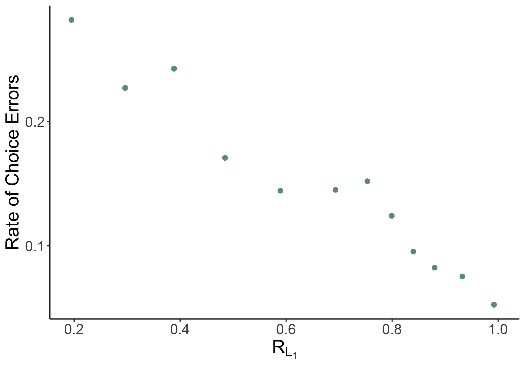
(a) Multiattribute

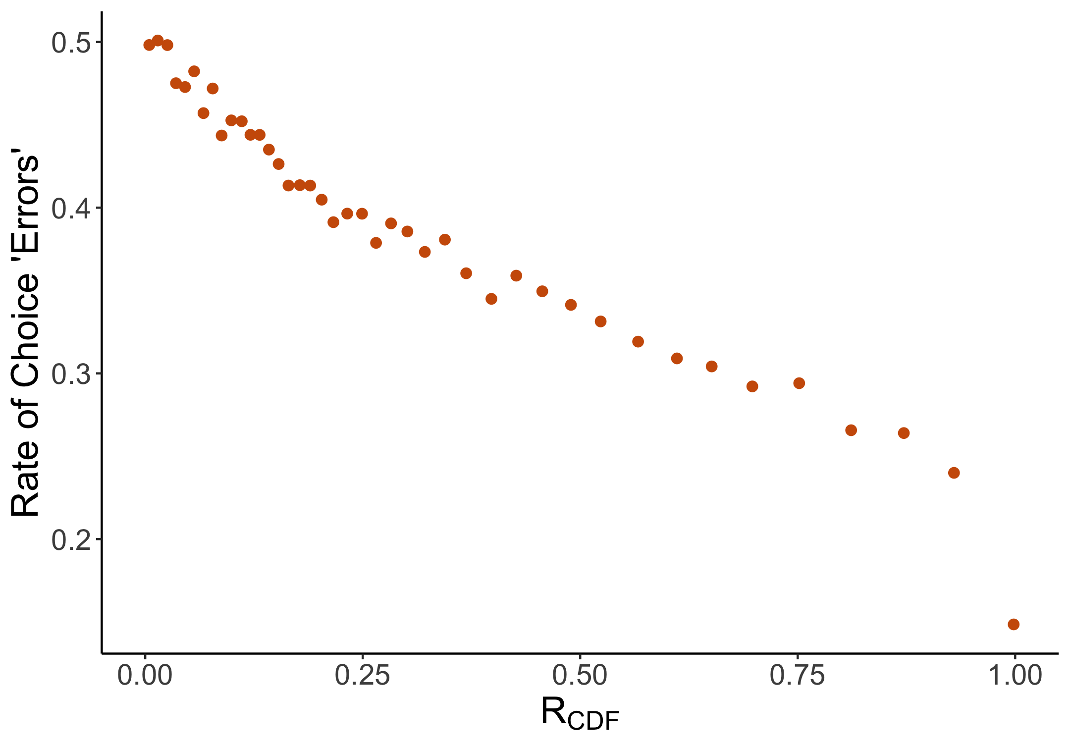
(b) Lottery

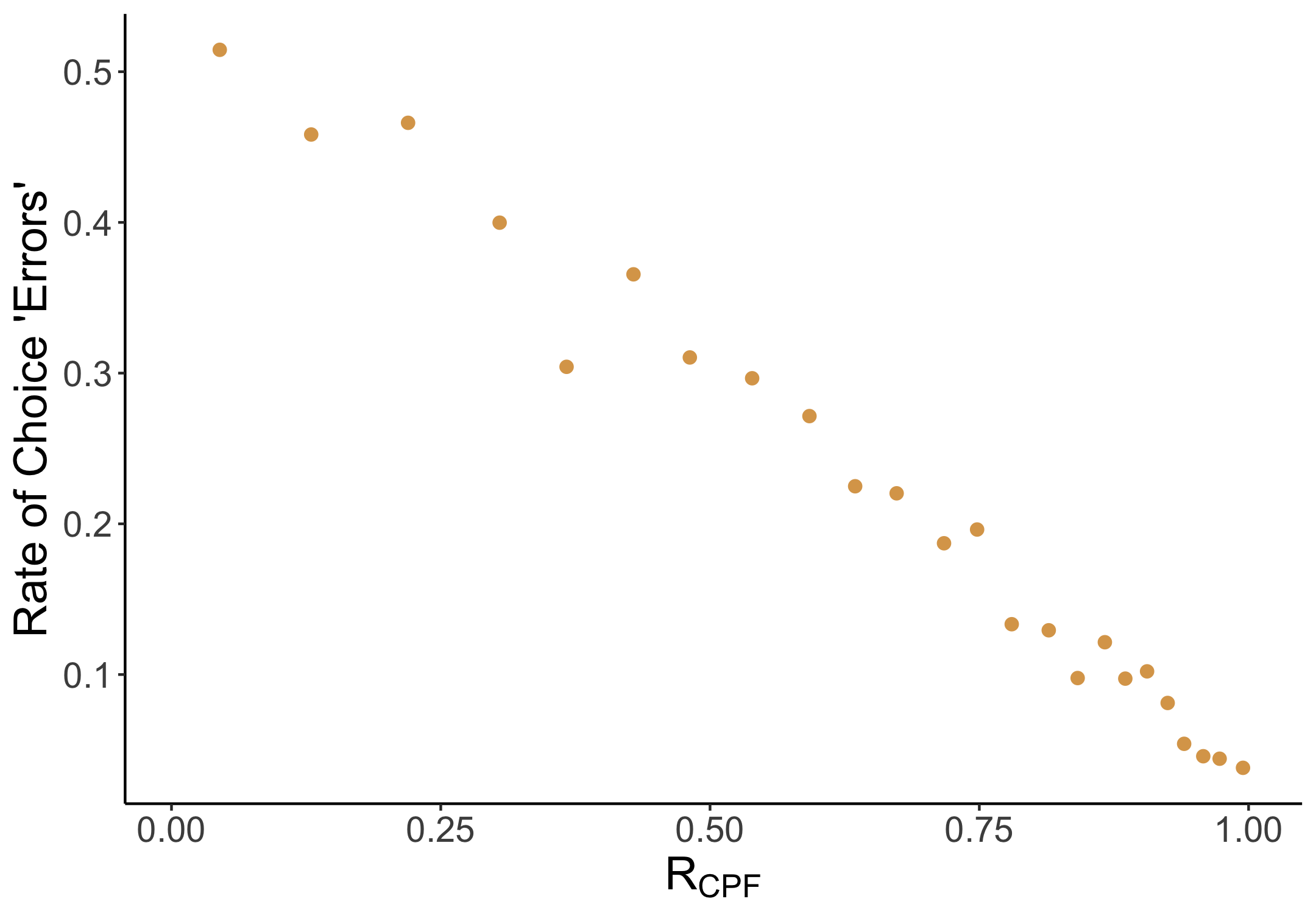
(c) Intertemporal

Figure 2: Binary Choice Rates vs. Complexity Measures. a) Plots the rate of choosing the lower valued option against our multiattribute complexity measure. b) Plots the rate of choosing the less-preferred option according to the best-fit expected utility model against our lottery complexity measure. c) Plots the rate of choosing the option with lower present value against our intertemporal complexity measure, where we use the best-fit discount factor to compute present value.

We find that the value-dissimilarity ratio is strongly predictive of choice “error" rates in all three domains, where we define an error as a) choosing the lower-value option in multiattribute choice and b) choosing the less-preferred option according to a best-fit model of risk and time preferences in lottery and intertemporal choice, respectively. This relationship is quantitatively large — in multiattribute choice, for instance, error rates range from 5% for choice problems with the highest value-dissimilarity ratio to more than 30% for choice problems with the lowest ratio. As we see in Figure 2, similarly pronounced relationships hold in intertemporal and lottery choice.

We also find that within-subject choice inconsistency is decreasing in the value-dissimilarity ratio across all three domains. In multi-attribute choice, inconsistency rates range from less than 5% for choice problems with the highest value-dissimilarity ratio to over 20% for choice problems with the lowest ratio, and we find similar relationships in lottery and intertemporal choice. Finally, we document that the value-dissimilarity ratio predicts not only comparison complexity revealed in choice behavior, but also captures subjective complexity, i.e., how hard comparisons actually feel to subjects. We find a strong decreasing relationship between cognitive uncertainty and the value-dissimilarity ratio.

Benchmarking predictive power. Using our experimental choice data, we benchmark the predictive power of our theory against existing models in all three domains. We structurally estimate a choice model in which choice rates depend only on the value-dissimilarity ratio. In multiattribute choice, our model delivers predictive power comparable to that of leading behavioral choice models while using fewer free parameters, and importantly explains a substantial amount of variation in choice that is not captured by existing models. In lottery and intertemporal choice, our model substantially outperforms leading behavioral choice models. In these domains, our model explains 10-28% more variation than the best alternative models without using any additional parameters (and in the case of lottery choice, actually using fewer parameters).

Multinomial choice model and behavioral implications. Having developed and tested our theory of comparison complexity, we embed the theory in a multinomial choice model to study its behavioral implications beyond binary choice. In our choice model, the decision-maker faces a menu of options, and chooses based on noisy signals on how each pair of options in the menu compares. In particular, for each comparison $(x,y)$ in the menu, the decision-maker generates a signal on the value comparison between the two options with precision $\tau_{xy}$, where $\tau_{xy}$ is governed by the value-dissimilarity ratio; the DM then chooses the option with the highest posterior expected value according to these signals.

Our choice model straightforwardly accounts for documented context effects in multinomial choice, such as the decoy and asymmetric dominance effects. Furthermore, we show that in lottery and intertemporal choice, our model rationalizes documented instabilities and biases in valuations, where here we formalize valuations within our choice model as a set of comparisons between an option and different amounts of money in a multiple price list. The core insight is that some risky or intertemporal prospects are easier to compare to money than others, which leads to systematic biases in valuations. Through this mechanism, our model predicts apparent probability weighting and hyperbolic discounting in valuations even in the absence of such distortions in direct choice, rationalizing documented preference reversals. The model also makes the novel testable prediction that one can reverse the direction of these biases by changing the numeraire in valuation: asking subjects to value lotteries using probability-equivalents, and intertemporal payments using time-equivalents.

Contribution and relation to prior work.

Our paper builds upon a growing literature on complexity and cognitive uncertainty in choice. These papers have documented how complexity can lead to noisy choice and/or systematically biased valuations (Enke and Shubatt,, 2023; Puri,, 2023, etc.), but typically focus on a single choice domain. Our unifying measure of complexity can be computed across several choice domains and experimental settings, offering a framework to tie together these disparate findings.

We also formalize insights from a more conceptual Psychology and Economics literature on similarity in choice. These papers (Rubinstein,, 1988; Tversky and Edward Russo,, 1969) use illustrative examples to argue that when agents choose between dissimilar objects, we may expect more violations of standard choice axioms. We both introduce an explicit similarity measure and formally model how similarity affects choice.

Finally, we bring cognitive insights and empirical evidence to a recently developing literature on stochastic choice. Our model belongs to a general class of moderate utility models axiomatized in He and Natenzon, (2023), wherein binary choice probabilities are a function of the value difference between two options normalized by their distance according to a metric. We make three contributions to this literature. First, we propose specific distance metrics in the domains of multiattribute, lottery, and intertemporal choice, motivated by the idea that the need to aggregate tradeoffs across option features governs the difficulty of comparison. Second, we provide a series of experimental tests of the model’s predictions, quantifying the tight relationship between the complexity measure and cognitive uncertainty, choice inconsistency, and choice errors. Third, we provide a novel and flexible framework for extending this class of binary choice models to multinomial choice.

Section 2 lays out the binary choice model and discusses the psychological motivation for the complexity measure. Section 3 describes the binary choice experiment design and results. Section 4 introduces the extension to multinomial choice, and applies the model to study context effects and valuations. Section 5 concludes. Proofs of all formal results are relegated to Appendix C.

2 Theory of Comparison Complexity

2.1 Binary Choice Framework

Let $X$ denote the set of options, and let $v_{x}$ denote the value of each $x\in X$. We consider a decision-maker (DM) who is uncertain over the value of each option in $X$, and when faced with a binary choice $\{x,y\}$, chooses based on a noisy signal on how $v_{x}$ and $v_{y}$ compare.

In particular, the DM has continuous, i.i.d. priors over $v_{x}$ for all $x\in X$ distributed according to a symmetric distribution $Q$, and observes a signal $s_{xy}$ on the ordinal value comparison between $x$ and $y$, given by

$$s_{xy} =\text{sgn}(v_{x}-v_{y})+\frac{1}{\sqrt{\tau_{xy}}}\epsilon_{xy},$$

$$\epsilon_{xy}\sim N(0,1)$$

and chooses the option with the highest posterior expected value. Here, the precision parameter $\tau_{xy}$ governs the ease of comparison between $x$ and $y$. Letting $\rho(x,y)$ denote the likelihood of choosing $x$ over $y$, this signal structure implies that $\rho(x,y)=P(\text{sgn}(v_{x}-v_{y})\tau_{xy})$, for some $P$ continuous, strictly increasing, with $P(t)=1-P(-t)$. That is, the decision-maker’s likelihood of correctly choosing the higher-valued option is increasing in the ease of comparison $\tau_{xy}$. In what follows, we propose a theory of how $\tau_{xy}$ depends on the structure of choice options in the domains of multiattribute, lottery, and intertemporal choice.

2.2 Comparison Complexity: General Principles

Our theory of $\tau_{xy}$ formalizes the intuition that the difficulty of a comparison is governed by the degree to which it requires the DM to aggregate tradeoffs. The theory is grounded in two principles that capture this intuition: similarity and dominance.

First, we posit holding fixed the value difference, options are easier to compare when they are more similar. Echoing previous work in psychology (Tversky and Edward Russo,, 1969) and in economics (Rubinstein,, 1988; He and Natenzon,, 2023), this property reflects the intuition that if options are more similar, the DM can divert attention from the features that are similar across the options and so more easily assess the differences between them, thereby reducing the need to aggregate tradeoffs. As such, we propose a representation of the ease of comparison $\tau_{xy}$ that is an increasing transformation $H$ of the value-dissimilarity ratio:

$$\tau_{xy}=H\left(\frac{|U(x)-U(y)|}{d(x,y)}\right),$$

where the numerator contains the value difference between the two options and the denominator is a distance metric measuring their dissimilarity.

Second, we posit options are maximally easy to compare when there is a dominance relationship between them. In the presence of dominance, the DM does not need to engage with trade-offs to see which option is better, and so we should expect comparisons that involve dominance to be easier those that do not. As formalized in the sections below, this principle gives rise to a specific distance metric in each domain, depending on the domain-relevant notion of dominance.

2.3 Multiattribute Choice

Consider the domain of multiattribute choice, where each option $x\in X_{1}\times...\times X_{n}$ is defined on $n$ real-valued attributes, where $X_{i}\in\mathbb{R}$. Utility is linear in attributes, where the value of each option $x$ is given by $v_{x}=U(x)=\sum_{k}\beta_{k}x_{k}$ for attribute weights $\beta\in\mathbb{R}^{n}$. We propose that the ease of comparison in this domain is governed by the following representation:

Definition 1.

Say that $\tau_{xy}$ has an $L_{1}$-complexity representation, denoted $\tau^{L1}_{xy}$, if there exists $\beta\in\mathbb{R}^{n}$, $\beta_{k}\neq 0$ for all $k$, such that

$$\tau_{xy}=H\left(\frac{|U(x)-U(y)|}{d_{L1}(x,y)}\right)$$

for $H$ continuous, strictly increasing with $H(0)=0$, where $d_{L1}(x,y)=\sum_{k}|\beta_{k}(x_{k}-y_{k})|$ is the $L_{1}$ distance between $x$ and $y$ in value-transformed attribute space.

In words, under the $L_{1}$-complexity representation, the ease of comparison between two options is governed by their value-dissimilarity ratio: their integrated value difference, normalized by a distance metric equal to their feature-by-feature value difference.

Note that our proposed complexity representation satisfies the properties of similarity and dominance. Holding fixed the value difference between two options, the ease of comparison is increasing in the similarity between $x$ and $y$, as measured by a distance metric on the space of alternatives. Moreover, if there is an attribute-by-attribute dominance relationship between $x$ and $y$; i.e. $\beta_{k}x_{k}\geq\beta_{k}y_{k}$ for all $k$, the ease of comparison $\tau_{xy}$ takes on its maximal value of $H(1)$.

$L_{1}$-complexity also satisfies a simplification property, wherein reducing the number of active attributes — that is, attributes along which there is a value difference — increases the ease of comparison. To take an example, suppose $n=3$, $\beta=(1,1,1)$, and consider the following comparisons:

$$\begin{array}[]{ll}&(x,y)\\ x&=(10,7,9)\\ y&=(3,15,5)\end{array}\qquad\begin{array}[]{ll}&(x^{\prime},y)\\ x^{\prime}&=(3,14,9)\\ y&=(3,15,5)\end{array}$$

Note that $(x^{\prime},y)$ is formed by eliminating the value difference along the first attribute and redistributing that value to the second attribute. Our complexity representation predicts that the DM finds $(x^{\prime},y)$ easier to compare than $(x,y)$, i.e. $\tau_{x^{\prime}y}>\tau_{xy}$. More generally, our model predicts that eliminating a value difference along some attribute $i$ and redistributing it to another attribute $j$ makes options easier to compare. This property again reflects tradeoff complexity: if individuals find it difficult to aggregate tradeoffs across features, we should expect that a simplification operation of the kind above, where some of that aggregation is done for the decision-maker, makes the comparison easier.

2.3.1 Axiomatic Foundations

The above properties are not only satisfied by our complexity representation, but are also key properties in its characterization. Our representation for $\tau_{xy}$ is characterized by axioms on binary choice behavior corresponding to the properties of similarity, dominance, and attribute simplification, along with three other easily understood axioms.

Let $\mathcal{D}=\{(x,y)\in\mathbb{R}^{n}\times\mathbb{R}^{n}:x\neq y\}$ denote the set of all pairs of distinct options. Consider a binary choice rule $\rho:\mathcal{D}\to[0,1]$ satisfying $\rho(x,y)=1-\rho(y,x)$ for all $x,y$; here, $\rho(x,y)$ denotes the likelihood of choosing $x$ over $y$. In our binary choice framework, $\tau_{xy}$ has an $L_{1}$-Complexity representation if and only if binary choice probabilities take the form below.

Definition 2.

Say that a binary choice rule $\rho$ has an $L_{1}$-Complexity Representation if there exists $\beta\in\mathbb{R}^{n}$, $\beta\neq 0$, such that

$$\rho(x,y)=G\left(\frac{U(x)-U(y)}{d_{L1}(x,y)}\right)$$

for some $G$ continuous, strictly increasing.

That is, under our representation for $\tau_{xy}$, the likelihood of choosing $x$ over $y$ is an increasing function of the signed value difference between the two options, normalized by their $L_{1}$ distance.

We now characterize our representation. Let $x_{\{k\}}y$ denote the option obtained by replacing the $k$th attribute of $y$ with $x_{k}$. Say that $x$ dominates $y$, written $x>_{D}y$, if $\rho(x_{\{k\}}y,y)\geq 1/2$ for all $k$ with a strict inequality for at least one $k$. Say that attribute $k$ is null if $\rho(x_{\{k\}}z,y_{\{k\}}z)=1/2$ for all $x,y,z\in X$. Consider the following axioms:

1. Continuity: $\rho(x,y)$ is continuous on its domain.

2. Linearity: $\rho(x,y)=\rho(\alpha x+(1-\alpha)z,\alpha y+(1-\alpha)z)$.

3. Moderate Transitivity: If $\rho(x,y)\geq 1/2$, $\rho(y,z)\geq 1/2$, then either $\rho(x,z)>\min\{\rho(x,y),\rho(y,z)\}$ or $\rho(x,z)=\rho(x,y)=\rho(y,z)$.

4. Dominance: If $x>_{D}y$, then $\rho(x,y)\geq\rho(w,z)$ for any $w,z\in X$, where the inequality is strict if $w\not>_{D}z$.

5. Simplification: For any $x,x^{\prime},y\in X$, satisfying for $i\neq j$

   $$x^{\prime}_{k}=\begin{cases}y_{i}&k=i\\ x^{\prime}_{j}&k=j\\ x_{k}&\text{ otherwise}\end{cases}$$

   for some $x^{\prime}_{j}\in X_{j}$: if $\rho(x,y)\geq 1/2$ and $\rho(x^{\prime},x)=1/2$, then $\rho(x^{\prime},y)\geq\rho(x,y)$.

Continuity and Linearity are standard axioms, and the latter reflects the fact that both preferences and the $L_{1}$ distance in our model are linear in attributes. Moderate Transitivity is a transitivity condition on binary choice that allows for choice probabilities to depend on features of choice options other than their value difference – and specifically allows for choice probabilities to depend on a notion of similarity between choice probabilities.

Dominance and Simplification are the exact counterparts of the properties of $\tau^{L1}_{xy}$ discussed earlier, stated in terms of choice probabilities. Dominance says that if $x$ is revealed better than $y$ on every attribute, then the likelihood of correctly choosing $x$ takes on its maximal value. Simplification says that if we eliminate the value difference between $x$ and $y$ along some attribute and redistribute that value to another attribute of $x$, the likelihood of correctly choosing $x$ increases.

The following theorem says that when there are 3 or more attributes, M1–M5 characterize the behavioral implications of our representation for binary choice data, and that the parameters $(G,\beta)$ of our representation can be identified from binary choice data.

Theorem 1.

Suppose that all attributes are non-null and $n>2$. $\rho(x,y)$ has a $L_{1}$-complexity representation $(G,\beta)$ if and only if it satisfies M1–M5. Moreover, if $\rho(x,y)$ also has a $L_{1}$-complexity representation $(G^{\prime},\beta^{\prime})$, then $G^{\prime}=G$ and $\beta^{\prime}=C\beta$ for $C>0$.

2.4 Risky and Intertemporal Choice

2.4.1 Lotteries

Consider the lottery domain, where each option $x$ is a finite-support lottery over $\mathbb{R}$; that is each $x$ is described by the mass function $f_{x}:\mathbb{R}\to[0,1]$ where $f_{x}(w)>0$ for finitely many $w$. Let $F_{x}$ and $F_{x}^{-1}$ denote the CDF and quantile function of $x$. Preferences are given by expected utility, with $v_{x}=EU(x)=\sum_{w}u(w)f_{x}(w)$ for $u$ strictly increasing.

Definition 3.

$\tau_{xy}$ has an CDF-complexity representation, denoted $\tau^{CDF}_{xy}$, if for $u$ strictly increasing,

$$\tau_{xy}=H\left(\frac{|EU(x)-EU(y)|}{d_{CDF}(x,y)}\right)$$

for $H$ continuous, strictly increasing with $H(0)=0$, where the CDF distance $d_{CDF}$ is given by

$$d_{CDF}(x,y)=\int_{0}^{1}|u(F^{-1}_{x}(q))-u(F^{-1}_{y}(q))|\,dq$$

As with the $L_{1}$-complexity representation, the ease of comparison between two options under the CDF-complexity representation is governed by their value-dissimilarity ratio — that is, the value difference between the two options normalized by a measure of their dissimilarity. The specific dissimilarity measure in our representation, $d_{CDF}(x,y)$, is a metric equal to the area between the utility-valued CDFs of $x$ and $y$, and so captures how similarly the payoffs in $x$ and $y$ are distributed.

This measure provides a formal foundation for existing empirical work which documents a tight connection between the CDF distance and choice rates. In particular, both Enke and Shubatt, (2023) and Erev et al., (2002) show that the performance of stochastic choice models over lotteries dramatically improves when decision noise is allowed to vary with the a special case of the CDF distance, with $u(x)=x$.

2.4.2 Intertemporal Payoff Flows

Now consider the intertemporal domain, where each option $x$ is a finite stream of time-dated payoffs; each $x$ is described by the payoff function $m_{x}:[0,\infty)\to\mathbb{R}$ where $m_{x}(t)\neq 0$ for finitely many $t$; $m_{x}(t)$ describes how much $x$ pays off at time $t$. Let $M_{x}(t)=\sum_{t^{\prime}\leq t}m_{x}(t^{\prime})$ denote the cumulative payoff function of $x$, which describes how much money $x$ pays in total up until time $t$. Preferences are given by exponential discounting, with $v_{x}=PV(x)=\sum_{t}\delta^{t}m_{x}(t)$, for $\delta<1$.

Definition 4.

$\tau_{xy}$ has an CPF-complexity representation, denoted $\tau^{CPF}_{x,y}$, if there exists $\delta<1$ such that

$$\tau_{xy}=H\left(\frac{|PV(x)-PV(y)|}{d_{CPF}(x,y)}\right)$$

for $H$ continuous, strictly increasing with $H(0)=0$, where the CPF distance $d_{CPF}$ is given by

$$d_{CPF}(x,y)=\ln(1/\delta)\int_{0}^{\infty}|M_{x}(t)-M_{y}(t)|\cdot\delta^{t}\,dt.$$

As with our previous complexity measures, the ease of comparison between two options under the CPF-complexity representation is governed by their value-dissimilarity ratio, where the dissimilarity measure $d_{CPF}(x,y)$ is a metric that is proportional to the present value of the difference between the cumulative payoff functions of $x$ and $y$, and captures how similarly $x$ and $y$ distribute their payoffs across time.

2.4.3 Shared Properties

Like our multiattribute complexity measure, $\tau^{CDF}_{xy}$ and $\tau^{CPF}_{xy}$ satisfy our core properties of similarity and dominance. Holding fixed the value difference, $\tau^{CDF}_{xy}$ and $\tau^{CPF}_{xy}$ are increasing in the similarity between $x$ and $y$, as measured by a distance metric on the space of alternatives, where this distance metric is chosen to so that $\tau_{xy}$ takes on its maximal value when there is a dominance relationship between $x$ and $y$. In particular, say that a lottery $x$ first-order stochastically dominates $y$ when $F_{x}(w)\leq F_{y}(w)$ for all $w$, and say that a payoff flow $x$ temporally dominates $y$ if if $M_{x}(t)\geq M_{y}(t)$ for all $t$ — that is, if $x$ will have paid out more in total than $y$ at any point in time. Notice that $\tau^{CDF}_{xy}$ takes on its maximal value of $H(1)$ when there is a first-order stochastic dominance relationship between lotteries $x$ and $y$, and $\tau^{CPF}_{xy}$ takes on their maximal value of $H(1)$ when there is a temporal dominance relationship between payoff flows $x$ and $y$.

$\tau^{CDF}_{xy}$ and $\tau^{CPF}_{xy}$ also satisfy analogs of the simplification property for $\tau^{L1}_{xy}$, which says that aggregating value differences across different features into the same feature makes options easier to compare. As formally stated in Appendix B.1, concentrating value differences from different percentile regions in the distribution of two lotteries $x$,$y$ into the same region increases the ease of comparison according to $\tau^{CDF}_{xy}$, and concentrating value differences from different time periods of two payoff flows $x,y$ into the same time period increases the ease of comparison according to $\tau^{CPF}_{xy}$.

2.4.4 Axiomatic Foundations

The binary choice behavior implied by $\tau^{CDF}_{xy}$ and $\tau^{CPF}_{xy}$ can be characterized using axioms analogous to M1—M5. In Appendix B.1, we show how the binary choice rules corresponding to $\tau^{CDF}_{xy}$ and $\tau^{CPF}_{xy}$ are characterized by five axioms: direct translations of Continuity, Linearity, Moderate Transitivity, and Dominance, and an analog of Simplification.

2.4.5 Connection to $L_{1}$ Complexity

Our complexity measures for risk and time not only share the same properties of our multiattribute measure, but can also be interpreted as extensions of $L_{1}$ complexity. We relegate discussion of the connection between CPF and $L_{1}$ complexity to the appendix, and discuss the connection between CDF and $L_{1}$ complexity below. CDF complexity is equivalent to $L_{1}$ complexity when applied to a common attribute representation of lotteries — specifically, the attribute representation that maximizes the ease of comparison according to $L_{1}$ complexity.

Consider the set of possible couplings of lotteries $x,y$ — that is, the set $\Gamma(x,y)$ of joint distributions $g(w_{x},w_{y})$ over payoffs such that $\sum_{w_{y}}g(w,w_{y})=f_{x}(w)$ and $\sum_{w_{x}}g(w_{x},w)=f_{y}(w)$ for all $w$. Note that each coupling $g$ induces an attribute representation of $x$ and $y$, in which the attributes are given by the set of joint utility-transformed payoff realizations in the support of $g$, weighted by the likelihoods of those payoff realizations under $g$.

To take an example, consider a lottery $x$ which pays $18 w.p. $20\%$, and $y$ which pays $12 w.p. $25\%$, and consider the attribute structures induced by two different couplings:

$$\begin{array}[]{l|l l l l}&60\%&20\%&5\%&15\%\\ \hline\cr x&u(0)&u(0)&u(18)&u(18)\\ y&u(0)&u(12)&u(12)&u(0)\end{array}\qquad\qquad\begin{array}[]{l|l l l l}&75\%&5\%&20\%\\ \hline\cr x&u(0)&u(0)&u(18)\\ y&u(0)&u(12)&u(12)\end{array}$$

The attribute structure on the left corresponds to a coupling in which the lotteries are uncorrelated, and the attribute structure on the right corresponds to a coupling that imposes positive correlation between the lotteries. For each attribute structure induced by $g$, we can compute the ease of comparison under $L_{1}$ complexity, given by

$$\tau^{L1}_{xy}(g)\equiv H\left(\frac{|\sum_{w_{x},w_{y}}g(w_{x},w_{y})(u(w_{x})-u(w_{y}))|}{\sum_{w_{x},w_{y}}|g(w_{x},w_{y})(u(w_{x})-u(w_{y}))|}\right)=H\left(\frac{|EU(x)-EU(y)|}{\sum_{w_{x},w_{y}}|g(w_{x},w_{y})(u(w_{x})-u(w_{y}))|}\right).$$

Proposition 1 says that the attribute structure $g$ that maximizes the ease of comparison according to $\tau^{L1}_{xy}(g)$ gives rise to exactly the CDF complexity representation.

Proposition 1.

$\underset{g\in\Gamma(x,y)}{\max}\tau_{xy}^{L1}(g)=H\left(\frac{EU(x)-EU(y)}{d_{CDF}(x,y)}\right)$.

Proposition 1 points to the following two-stage cognitive interpretation of our CDF complexity measure: in a “representation stage", the DM first represents the lotteries using a common set of attributes, and then compares the lotteries along these attributes in an “evaluation stage". In particular, Proposition 1 says that if the DM represents the lotteries using an attribute structure that maximizes their comparability in the evaluation stage, where this ease of comparison is governed by $L_{1}$-complexity, the overall ease of comparison will be given by CDF complexity.

As with our lottery complexity measure, CPF complexity can be seen as an extension of $L_{1}$ complexity to intertemporal choice. In Appendix B.2, we show how the CPF complexity representation can be similarly derived as the $L_{1}$ complexity for the common attribute representation of intertemporal payoff flows that maximizes their ease of comparison.

2.5 Parameterizing the Model

In each of our domains, our model predicts that the the probability of choosing option $x$ over $y$ is given by

$$\rho(x,y) =G\left(\frac{U(x)-U(y)}{d(x,y)}\right),$$

where the signed value-dissimilarity ratio $\frac{U(x)-U(y)}{d(x,y)}$ is specified in each domain according to Definitions 1,3, and 4, and $G$ is a strictly increasing transformation that is symmetric around $0$, with $G(r)=1-G(-r)$. To obtain quantitative predictions, the analyst needs to specify the preference parameters that enter the value-dissimilarity ratio — the attribute weights $\beta$ in multiattribute choice, the Bernoulli utility function $u$ in lottery choice, and the discount factor $\delta$ in intertemporal choice — as well as the transformation $G$. In each domain, these objects can identified from binary choice data, as demonstrated in Theorem 1 for multiattribute choice, and in Appendix B.1 for our other two domains.

When fitting our model to data, as in Section 3, our preferred specification of $G$ is given by the two-parameter functional form

$$G(r)=\begin{dcases}(1-\kappa)-(0.5-\kappa)(1-r)^{\gamma}&r\geq 0\\ \kappa+(0.5-\kappa)(1+r)^{\gamma}&r<0\end{dcases}$$ (1)

Here $\kappa$ is a tremble parameter that governs the DM’s error rate at dominance, and $\gamma$ governs the curvature in the relationship between choice probabilities and the value-dissimilarity ratio. Note that for $\gamma<1$, error rates will be concave in $|r|$, which captures the possibility that the difficulty of a comparison may be steeply increasing away from dominance.

Note that $\gamma<1$ also implies that choice rates will be relatively insensitive to the value-dissimilarity ratio at indifference (i.e. at $r=0$) whereas psychometric evidence typically finds that accuracy rates are $S$-shaped in the difference between stimuli in unidimensional stimulus comparison tasks, and are therefore most sensitive to the differences between stimuli when they are close to equality (Woodrow,, 1933; Gescheider,, 2013). As such, we will also consider a three parameter functional form,

$$G(r)=\begin{dcases}(1-\kappa)-(0.5-\kappa)\frac{(1-r)^{\gamma}}{(r^{\psi}+(1-r)^{\psi})^{1/\psi}}&r\geq 0\\ \kappa+(0.5-\kappa)\frac{((1+r)^{\gamma}}{r^{\psi}+(1-r)^{\psi})^{1/\psi}}&r<0\end{dcases}$$ (2)

where the additional parameter $\psi$ governs the sensitivity of choice rates to $r$ around indifference. Note that when $\psi=1$, (2) reduces to (1).

3 Experimental Tests

We test our proposed representations of comparison complexity against data from three analogous binary choice experiments in multiattribute, intertemporal, and lottery choice. We first provide an overview of the goals and design features shared across the three experiments, and then present domain-specific details along with results.

3.1 Overview

The goals of these experiments are two-fold. First, we want to show that our proposed complexity ratios capture the difficulty of comparisons. In particular, our theory predicts that (1) choice errors, (2) choice inconsistency, and (3) subjective uncertainty, three natural indicators of choice complexity, should all be decreasing in the value-dissimilarity ratio. We show that our ratios are highly predictive of all three. Second, we want to show that even in relatively simple decision contexts, our model captures quantitatively important features of choice that are missed by standard models. We show that despite having a comparable number of or in some cases far fewer free parameters, our structurally estimated choice model is able to explain observed choice rates 20-30% better than leading behavioral models in the domains of lottery and intertemporal choice, and predicts variation in choice not captured by the best-fit behavioral model in multiattribute choice.

We address these questions in three parallel experimental datasets. We run new experiments in multi-attribute and intertemporal choice and compile existing data from Enke and Shubatt, (2023) and Peterson et al., (2021) to study risky choice. In our experiments, we recruit participants through an online survey platform to make 50 incentivized binary choice problems. For each problem, we elicit participants’ subjective certainty in their response. In order to measure choice consistency, 10 of these problems are randomly repeated throughout the survey. We collect an average of 37 choices for each of 662 multi-attribute choice problems and 1,100 intertemporal problems – a total of more than 66,000 individual decisions. Our compiled risk dataset includes nearly 10,000 problems (over 1 million decisions) and includes similar measures of cognitive uncertainty and consistency.

3.2 Multiattribute Choice

We ask participants to identify the cheaper of two hypothetical phone plans characterized by either two, three, or four attributes. These attributes include a device cost, a monthly flat fee, a data usage fee, and a quarterly wi-fi fee. Participants learn about a fictional consumer with a fixed budget and are asked to choose the plan that will save the consumer the most money over one year. The consumer’s data usage is known, and so each problem has an objectively payoff-maximizing answer, allowing us to perfectly observe choice errors. For three-attribute problems, the budget is $700 and the average plan costs $621. We fix the plans’ value difference at one of two values ($46 or $69) so that variation in the $L_{1}$ ratio mostly reflects variation in option similarity. If a participant is selected to earn a bonus (1 in 2 chance), we select one of their choices at random and pay them 1/12 of the money they saved. These payments range between $4 and $9. For more detail on the design and pre-registration, see Appendix D.

Figure 3 shows binned scatter plots relating the ratio (x-axis) to choice errors, cognitive uncertainty, and inconsistency. We see that all three are strongly decreasing in the ratio. The average error rate, only around 5% for problems near-dominance, increases five-fold for problems with the lowest values of the $L_{1}$ ratio ($R^{2}=0.32$). We take this as strong evidence that (1) the ratio indeed captures cognitive complexity, and (2) decision-makers respond to this complexity by making more random choices.

(a) Errors

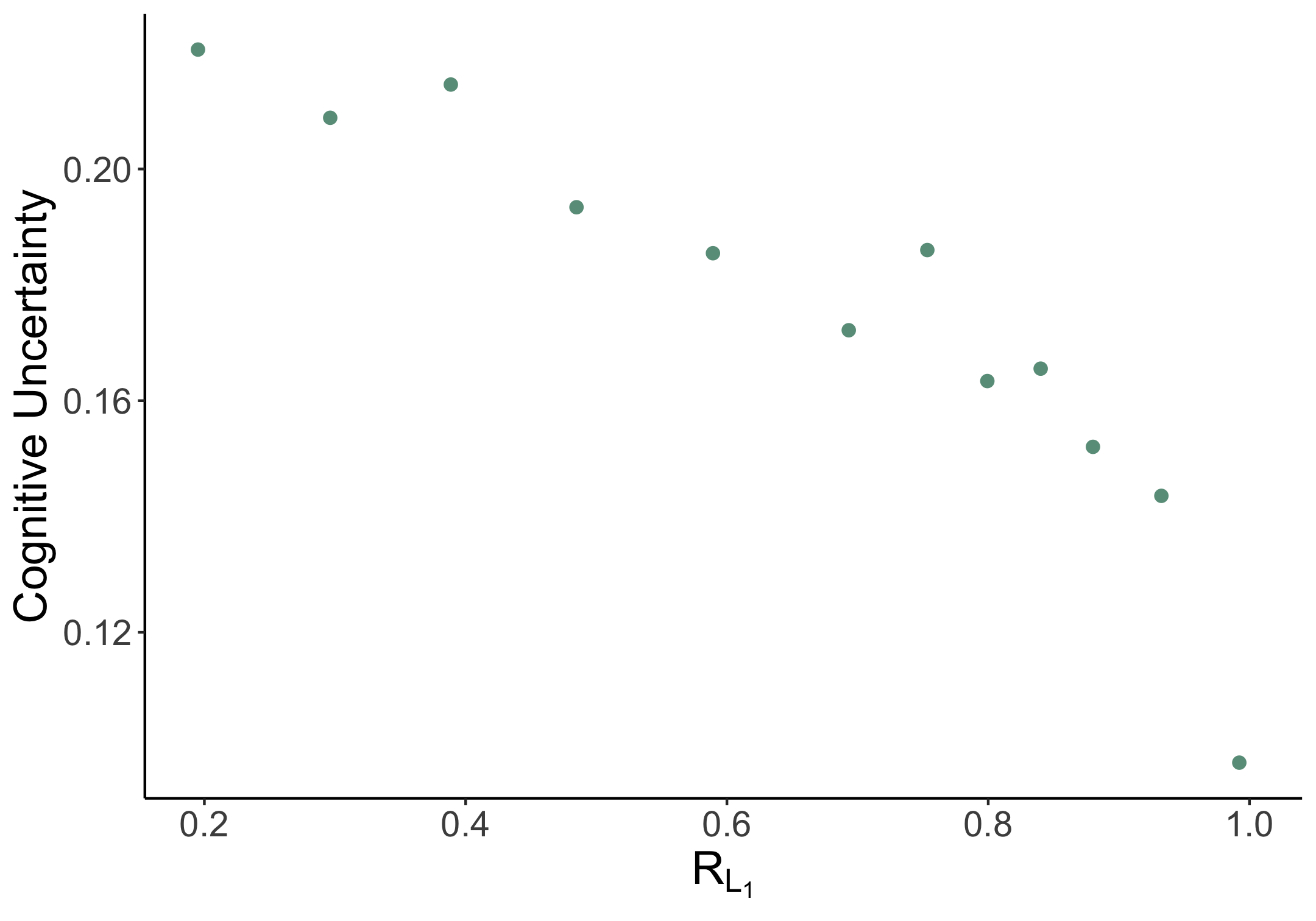
(b) Uncertainty

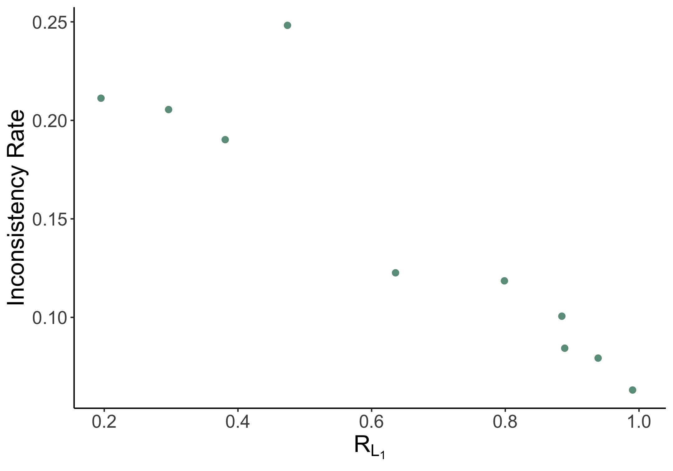
(c) Inconsistency

Figure 3: Error rates, cognitive uncertainty, and choice inconsistency in multi-attribute choice. Each of the 12 points summarizes approximately 48 problems.

Importantly, these relationships are not driven by variation in the value difference alone, but instead by variation in the $L_{1}$ ratio, which we varied independently of the value difference when constructing the choice problems. The regression evidence in Appendix Table 2 shows that the relationships above are unchanged when including controls for the value difference.

3.2.1 Benchmarking Performance

To study whether our theory explains variation in choice patterns that are not captured by existing behavioral models of multiattribute choice, we conduct a benchmarking exercise in which we structurally estimate our choice model, using the parameter specifications in (1) and (2), and compare its performance to leading behavioral multiattribute choice models, which we also structurally estimate on our data. We estimate three such models, each of which deliver accounts of how various biases lead to under- or overweighting of attributes in choice: salience-weighting (Bordalo et al.,, 2013), focusing (Kőszegi and Szeidl,, 2013), and relative thinking (Bushong et al.,, 2021), each with logit errors (see Appendix E.1 for details on the structural models).

Appendix Table 4 summarizes the estimation results. In predicting choice rates at the problem level, the fitted salience, focusing, and relative thinking models achieve $R^{2}$ values of .001, .001, and 0.35, respectively. Despite having one fewer free parameter than the relative thinking model, the two-parameter version of our choice model delivers a comparable $R^{2}$ of 0.29. Importantly, our model explains a substantial amount of variation in choice data not captured by the relative thinking model; as Appendix Table 5 documents, when regressing actual choice rates vs. fitted choice rates under the relative thinking model, including the fitted choice rates under our choice model as an additional predictor results in an increase in $R^{2}$ from 0.35 to 0.41, a 19% increase in variance explained.

3.3 Intertemporal Choice

We ask participants to choose which of two time-dated payoff streams they would prefer to receive. Each option has one or two payoffs, ranging between $1 and $40, to be received at delays ranging between the present and 2 years in the future. If the subject wins a bonus (1 in 5 chance), they will actually receive one of the payment streams they selected on the specified dates. For more details on the design and pre-registration, see Appendix D.

Unlike in multi-attribute choice, we cannot observe choice errors here – the definition of an “error” depends on the decision-maker’s discount function, which is unknown. The CPF ratio also depends on this discount function, so we proceed by experimentally estimating a representative agent exponential discount factor $\delta$ from the choice data. We estimate the choice model with additive logit errors, which yields a monthly discount factor of 0.93. For details on the specification, see Appendix E.1. In Figure 4, we present the main results from the intertemporal experiment. Here, a choice is coded as an “error” if an individual chooses the option with lower present value according to the estimated discount factor. As in our multiattribute choice data, we find very strong relationships between the CPF ratio and choice “errors,” cognitive uncertainty, and inconsistency. The average "error" rate ranges from around 5% for problems with the highest value of the CPF ratio to 50% for problems with the lowest value of the CPF ratio ($R^{2}=0.6)$. As the regression evidence in Appendix Table 6 documents, these relationships are virtually quantitatively unchanged when controlling for the value difference, which indicates that the ratio between the value difference and our proposed dissimilarity measure — as opposed to the value difference alone — is driving these relationships.

(a) “Errors”

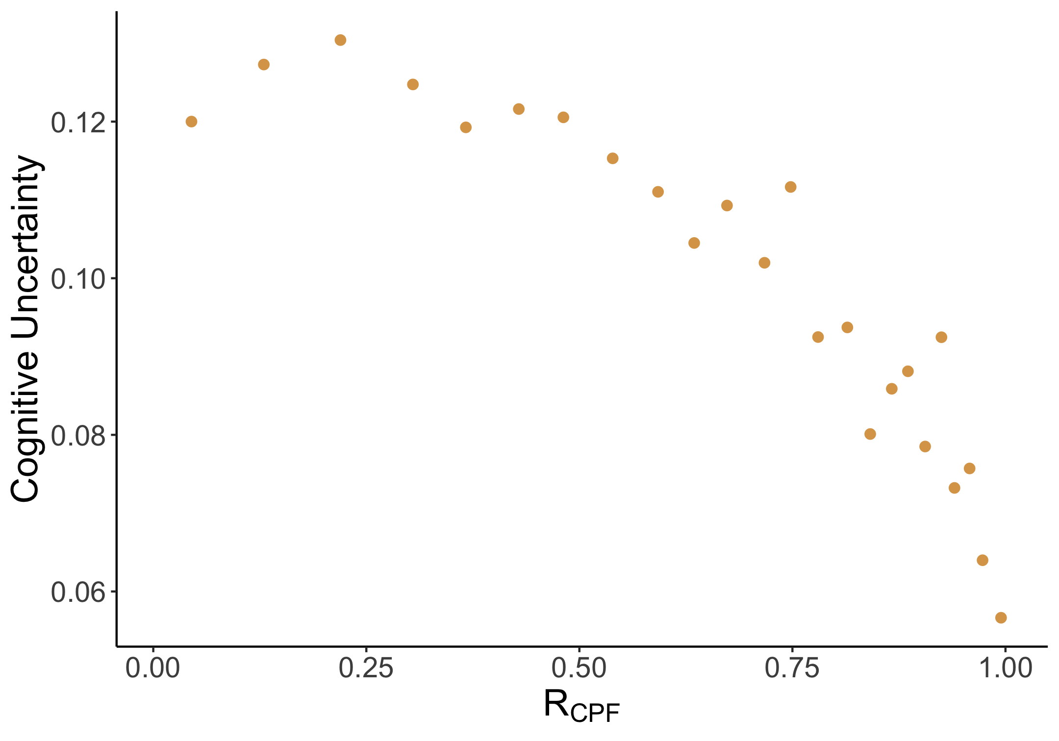
(b) Uncertainty

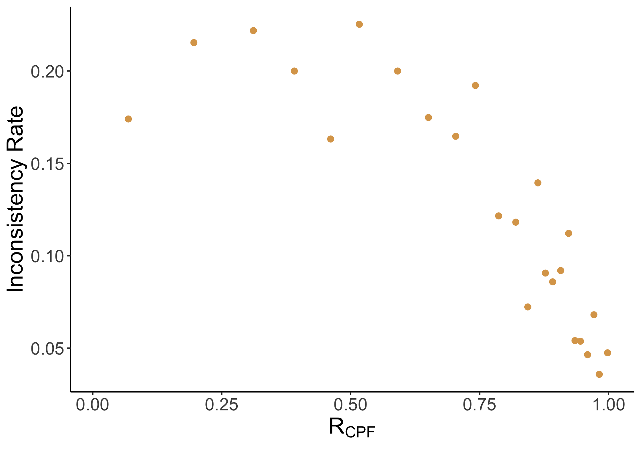
(c) Inconsistency

Figure 4: “Error” rates, cognitive uncertainty, and choice inconsistency in intertemporal choice. Each point summarizes approximately 44 problems.

3.3.1 Heterogeneity

In principle, the “errors” plotted in Figure 4(a) could reflect heterogeneous preferences. The inconsistency and cognitive uncertainty results suggest that this cannot be the entire story, as these measures are all within-subject, and do not depend on estimated preferences. Moreoever, we can perform the error analysis using individual-level discount factors $\delta_{i}$, which we estimate using the 50 choices observed for each subject. Using these individually estimated discount factors, we find a similarly pronounced relationship between the CPF ratio and apparent errors (see Appendix Figure 10 and Table 7).

3.3.2 Benchmarking Performance

While Figure 4 indicates that our model is a good descriptor of choice, but leaves open the question over whether the value-dissimilarity ratio explains meaningful variation in choice behavior that is not captured by other models. To this end, we conduct a benchmarking exercise analogous to that in Section 3.2.1 in which we structurally estimate our choice model, using the parameterization specified in (1), and compare its performance to leading intertemporal choice models. We estimate two such models: standard exponential discounting and hyperbolic discounting, both with logit errors (see Appendix E.2 for details on the structural models). In predicting choice rates at the problem level, these models achieve $R^{2}$ values of 0.75 and 0.78 respectively. In contrast, our model achieves an $R^{2}$ of 0.88 – a 13% improvement in variance explained over hyperbolic discounting, using the same number of parameters. Appendix Table 8 summarizes the estimation results.

3.4 Lottery Choice

In both lottery choice experiments, participants were asked to choose between two lotteries which pay off different amounts with known probabilities. If participants were selected to receive a bonus, the computer would simulate one of their chosen lotteries and actually pay out the simulated value. As in intertemporal choice, both the CDF ratio and our notion of choice “errors” depend on an unknown preference parameter – the Bernoulli utility function. We proceed by estimating a representative-agent model of CRRA utility with additive logit errors (see Appendix E.3 for details), and code “errors” as departures from this estimated model. Figure 5 shows the results. Once again, all three outcomes are strongly decreasing in the ratio; in particular, the CDF ratio achieves an $R^{2}$ of 0.45 in variance explained over error rates. Consistent with our results in our other two domains, these relationships are driven by the value-dissimilarity ratio, as opposed to the value difference alone: as Appendix Table 9 demonstrates, the relationships below are quantitatively similar when including controls for the value difference.

(a) “Errors”

(b) Uncertainty

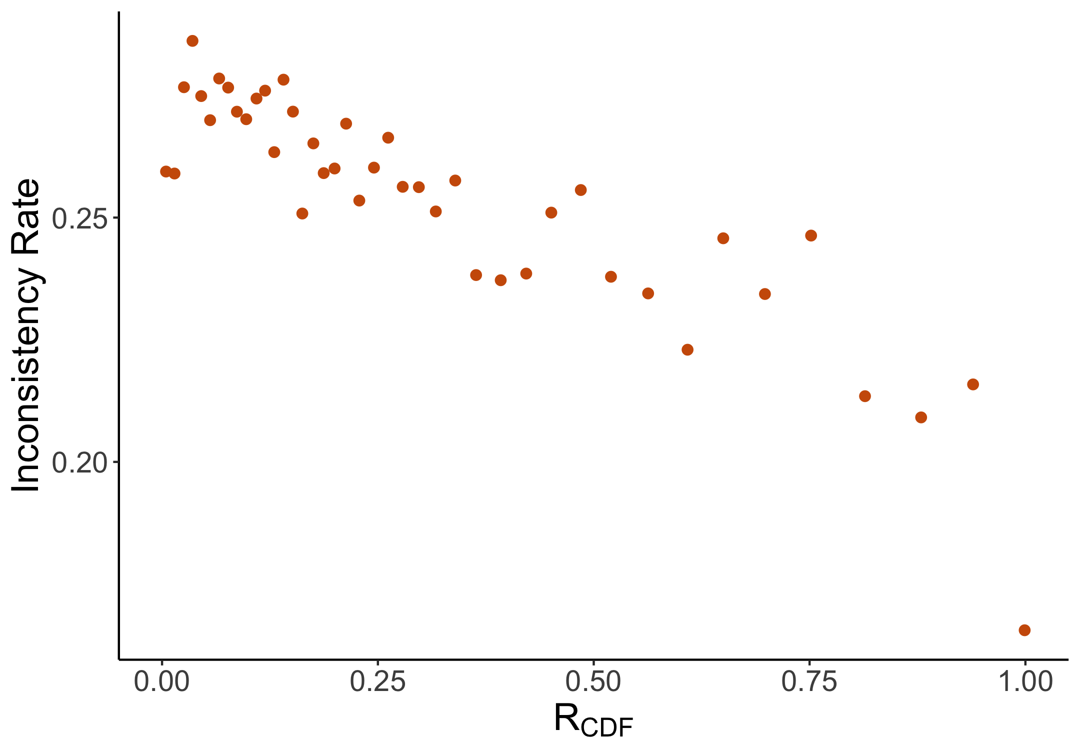
(c) Inconsistency

Figure 5: “Error” rates, cognitive uncertainty, and choice inconsistency in lottery choice.

3.4.1 Heterogeneity

As in intertemporal choice, we can recreate the error analysis using individual-level risk aversion parameters $\alpha_{i}$, which we estimate using the 50 lottery choices observed for each individual in the data collected in Enke and Shubatt, (2023). Using these individually estimated risk aversion parameters, we find if anything a stronger relationship between the CPF ratio and apparent errors (see Appendix Figure 11 and Table 10).

3.4.2 Benchmarking Performance

As with intertemporal choice, our model explains significant variation in choice rates uncaptured by existing rational and behavioral choice models. To benchmark performance, we estimate a standard reference-dependent expected utility model as well as a full prospect theory model with loss aversion (see Appendix E.3 for details). We compare the performance of these models to two versions of our CDF complexity model, both of which use the paramterization of $G$ specified in (1): one that assumes risk neutral preferences, and one that allows for utility curvature, jointly estimated along with the parameters for $G$ (see Appendix E.3 for details).

Appendix Table 11 summarizes the estimation results. In predicting choice rates at the problem level, reference dependent expected utility and prospect theory achieve $R^{2}$ values of 0.56 and 0.59 respectively. Despite having four fewer parameters than prospect theory, the risk-neutral version of our model achieves an $R^{2}$ of 0.66 – a 12% improvement in variance explained over prospect theory. This is in line with results from Enke and Shubatt (2023), who find that allowing complexity to enter the noise term of a logit choice model substantially improves performance over standard models. Adding an additional parameter to capture utility curvature in our model yields an $R^{2}$ of 0.73 – a 24% improvement in variance explained over prospect theory.

4 Multinomial Choice

We have thus far focused on comparison complexity in binary choice. We now extend our model to multinomial choice and show how comparison complexity can rationalize a range of documented anomalies in choice and valuation, such as context effects, preference reversals, and apparent biases in the valuation of risky and intertemporal prospects.

4.1 Multinomial Choice Extension

Consider the same setting as in our binary choice framework. There is a set of options $X$, and the DM has continuous, iid priors over $v_{z}$ for all $z\in X$, distributed according to a symmetric distribution $Q$. Let $\mathcal{M}$ denote the collection of finite subsets of $X$, and let $\mathcal{A}=\{A\in\mathcal{M}:|A|\geq 2\}$ denote the set of finite menus. The DM faces a choice problem $(A,C)\in\mathcal{A}\times\mathcal{M}$, comprised of a menu of options $A$ and a choice context $C$ – a set of options the DM observes but cannot choose, i.e. phantom options. The DM chooses from $A$ based on signals on how each pair of options in $A\cup C$ compare.

In particular, for each pair of distinct options $x,y\in A\cup C$, the DM observes a signal of the form

$$s_{xy} =\text{sgn}(v_{x}-v_{y})+\frac{1}{\sqrt{\tau_{xy}}}\epsilon_{xy},$$

$$\epsilon_{xy}\sim N(0,1)$$

Letting $s$ denote the collection of these signals, the DM chooses the option $x\in A$ with the maximal posterior expected value $E[v_{x}|s]$. We are interested in the resulting choice probabilities in a choice problem, which are given by

$$\rho(x,A|C)=\mathbb{P}(\{s:E[v_{x}|s]>E[v_{y}|s]\,\forall\,y\in A/\{x\}\})$$

Note that the restriction of this choice model to binary choice problems, i.e. $(A,C)$ such that $|A|=2$ and $C=\varnothing$, is exactly the binary choice model studied in Section 2. With some abuse of notation, we will let $\rho(x,y)=\rho(x,\{x,y\}|\varnothing)$ denote binary choice probabilities, and let $\rho(x,y|C)=\rho(x,\{x,y\}|C)$ denote binary choice probabilities given a choice context $C$.

Discussion of model properties. As this model extends our binary choice framework, it delivers the prediction that binary choices are unbiased – that is, the DM always picks the higher-valued option weakly more often in binary choice problems. In choice from larger menus, however, the presence of comparisons to other options in the menu or choice context can lead to systematic distortions in choice.

To illustrate, consider an example where $X=\{x,y,z\}$, with $v_{x}>v_{y}>v_{z}$ and where $\tau_{xy}=\tau_{xz}=0$, $\tau_{yz}=\infty$. That is, the DM has no idea how $x$ compares to $y$ and $z$, but knows that $y$ is better than $z$. Here, the model predicts that $\rho(y,x|\{z\})=0$ – the presence of $z$ in the choice context provides additional information that rules out posterior beliefs over $(v_{x},v_{y},v_{z})$ in which $v_{y}<v_{z}$, thus distorting the the DM’s choice in favor of the inferior option $y$. In Section 4.2, we show how the model can rationalize a number of documented context effects using this logic.

To apply the choice model in a given domain, the analyst needs to specify the ranking of the choice options according to $v_{z}$ as well as the precision parameters $\tau_{xy}$. While these primitives can be identified using binary choice behavior, as we show in Appendix B.4, our approach in the remainder of this section will be to discipline the model using our theory of comparison complexity, which pins down the primitives $v_{x}$ and $\tau_{xy}$ in the domains of multiattribute, lottery, and intertemporal choice.

Relationship to Existing Models. Our model belongs to class of menu-dependent learning models (e.g. Safonov,, 2022; Natenzon,, 2019), in which the DM chooses based on a signal that depends on the menu that she faces. One model in this class that warrants discussion is the Bayesian Probit model in Natenzon, (2019). In this model, the DM has i.i.d. Gaussian priors over $v_{x}$, and chooses based on signals $s_{x}=v_{x}+\frac{1}{p}\epsilon_{x}$ received for each option in the menu, where the $\epsilon_{x}\sim N(0,1)$ are jointly normal across options. The pairwise correlations of $(\epsilon_{x},\epsilon_{y})$ allow the model to capture a notion of the ease of comparability between choice options, where choice options are more easily comparable if $(\epsilon_{x},\epsilon_{y})$ are more highly correlated.

Recall that in our model, the DM only receives information on ordinal value comparisons. In Bayesian Probit, the DM learns about the cardinal value differences between choice options, which rules out certain intuitive choice patterns. For instance, consider the the following choice options in the multiattribute domain:

$$x =(11,0)$$

$$y =(0,10)$$

$$z =(0,0)$$

Since $z$ is dominated by both $x$ and $y$, we might expect that $\rho(x,z)=\rho(y,z)=1$ and also $\rho(x,y)<1$; that is, the DM does not err in the presence of dominance but finds tradeoffs across attributes difficult. Bayesian Probit cannot rationalize this choice data; $\rho(x,z)=\rho(y,z)=1$ implies that $\operatorname{\text{Cor}}(\epsilon_{x},\epsilon_{z})=\operatorname{\text{Cor}}(\epsilon_{y},\epsilon_{z})=1$, which implies $\operatorname{\text{Cor}}(\epsilon_{x},\epsilon_{y})=1$. This yields the counterfactual prediction $\rho(x,y)=1$.

Intuitively, in Bayesian Probit the DM receives information on the cardinal value difference between choice options. As such, when the Bayesian Probit DM perfectly learns the cardinal value differences $v_{x}-v_{z}$ and $v_{y}-v_{z}$, they also learn the value difference $v_{x}-v_{y}$. In our model, on the other hand, the DM only receives information on the ordinal value comparison between choice options, which allows for situations in which the DM perfectly learns that $v_{x}>v_{z}$ and $v_{y}>v_{z}$, yet remains uncertain regarding the ranking between $v_{x}$ and $v_{y}$.

4.2 Context Effects

In our model, the presence of other options in the choice context can generate information that distorts choice, even if these options are never chosen. The following proposition summarizes this prediction.

Proposition 2.

Let $v_{x},v_{y}>v_{z}$. If $\tau_{yz}>\tau_{xz}$, there exists $\epsilon>0$ such that if $\tau_{xy}<\epsilon$, $\rho(y,x|\{z\})>1/2$.

Proposition 2 says that when an inferior option $z$ is easier to compare to $y$ than to $x$, the presence of $z$ in the choice context will distort choice in favor of $y$ if $x$ and $y$ are sufficiently hard to compare. Intuitively, if the DM does not know how $x$ compares to $y$ or $z$, but learns that $y$ is in fact better than $z$, the presence of $z$ can push choice in favor of $y$ – even when $x$ is strictly better than $y$. When combined with our theory of comparison complexity in the multiattribute domain, the above result rationalizes familiar decoy and asymmetric dominance effects.

Corollary 2.1.

Consider options from $X=\mathbb{R}^{n}$, with $v_{x}=\sum\beta_{k}x_{k}$ and let $\tau_{xy}$have an $L_{1}$-complexity representation. Let $v_{x},v_{y}>v_{z}$.

1. If $v_{x}=v_{y}$, then $d_{L1}(x,z)>d_{L1}(y,z)$ implies $\rho(y,x|\{z\})>1/2$.

2. For any value difference $\Delta=|v_{x}-v_{y}|$, there exists $\underline{d}\in\mathbb{R}^{+}$ such that if $d_{L1}(x,y)>\underline{d}$, there exists $z\in X$ with $d_{L1}(x,z)>d_{L1}(y,z)$ such that $\rho(y,x|\{z\})>1/2$.

Part (i) says that if $x$ and $y$ are indifferent, then introducing an inferior phantom option $z$ that is more similar to $y$ than $x$ distorts choice in favor of $y$. Part (ii) says this distortion does not just arise at indifference: if $x$ and $y$ are sufficiently dissimilar relative to their value difference, there exists a decoy $z$ that distorts choice in favor of $y$.

Example 1.

(Classic decoy effects). Consider a setting where options have two attributes, where $\beta=(1,1)$, and where $\tau_{xy}$ has an $L_{1}$ complexity representation. Consider two indifferent choice options $x=(1,2)$, $y=(2,1)$, and consider the effect of including a phantom option on choice shares between $x$ and $y$.

Case 1: $z=(1.8,0.8)$. Since $d_{L1}(x,z)<d_{L1}(y,z)$, we have $\rho(y,x|\{z\})>0.5$. We recover the classic asymmetric dominance effect: the addition of an option that is dominated by the target option $y$ but not by the competitor $x$ distorts choice in favor of $y$.

Case 2: $z^{\prime}=(1.5,1.1)$. We again have $d_{L1}(x,z^{\prime})<d_{L1}(y,z^{\prime})$, we have $\rho(y,x|\{z^{\prime}\})>0.5$. Here, the model predicts a “good deal" effect – $z^{\prime}$ is not dominated by either $x$ or $y$, but its proximity to $y$ makes the target option seem like a “good deal" relative to $z$, whereas its distance to $x$ prevents the DM from drawing the same inference about the competing option.

Case 3: $z^{\prime\prime}=(0.8,0.5)$. Here, $d_{L1}(x,z^{\prime\prime})=d_{L1}(y,z^{\prime\prime})$, and so Corollary 2.1 implies that $\rho(y,x|\{z^{\prime\prime}\})=0.5$. That is, the model predicts that the addition of a mutually dominated option does not affect choice shares.

Comparison to other context-dependence models. Though each of the choice patterns above can be explained by familiar models, our model is distinct in simultaneously explaining all three. The salience (Bordalo et al.,, 2013) and focusing models (Kőszegi and Szeidl,, 2013) cannot rationalize the decoy effects in Cases 1 and 2. The relative thinking model (Bushong et al.,, 2021), in which the DM weighs a given change along an attribute by less when there is a larger range of values along that attribute, can rationalize the decoy effect in Case 1 as a result of option $z$ extending the range of attribute 2 more than attribute 1, but not Case 2, where $z^{\prime}$ has no effect on attribute ranges. The pairwise normalization model (Landry and Webb,, 2021) predicts that $z$ increases the relative of $y$ relative to $x$ whenever $z_{1}/z_{2}$ is closer to $y_{1}/y_{2}$ than it is to $x_{1}/x_{2}$, and so can rationalize the decoy effects in both Cases 1 and 2, but also delivers the counterfactual prediction that the addition of a mutually dominated option $z^{\prime\prime}$ will also distort choice in favor of $x$. Furthermore, all of these models are formulated in multi-attribute choice, which means they cannot easily explain documented decoy effects in lottery choice (Soltani et al.,, 2012) or other domains. Our choice framework straightforwardly applies to lottery and intertemporal choice.

We also make an important conceptual distinction from these existing models. In our model, biased choice does not arise from a behavioral bias, but instead as a rational response to imperfect comparability. We only expect decoy options to distort choice between $x$ and $y$ when their binary comparison is challenging. This is consistent with the fact that the attraction effect is muted when consumers face familiar choice contexts or have clear prior preferences (Huber et al.,, 2014) – an empirical phenomenon that is not well-explained by existing models.

4.3 Biases and Instabilities in Valuation

Consider the classic preference reversal phenomenon in risky choice. Lottery $x$ pays a high amount with a low probability, while $y$ pays a modest sum with a high probability, e.g.

$$x:\quad\$14\text{ with 28\%}$$

$$y:\quad\$4\text{ with 98\%}$$

We consistently see that most subjects choose $y$ over $x$ in direct choice between the two, but state a higher certainty equivalent for $x$ when valuing the two lotteries independently. A number of explanations for these apparent preference reversals have been put forth in the literature, such as intransitive preferences or violations of independence (see Seidl, (2002) for a review). Our model makes two simple predictions which together rationalize preference reversals. First, valuations are systematically biased when options are difficult to compare to money; and second, some options are easier to compare to money than others.

4.3.1 Modeling Valuations

To model valuations, we extend our multinomial choice framework as follows. The DM now faces a finite menu sequence $A^{1},A^{2},...,A^{n}\in\mathcal{A}$ in a choice context $C$, generates a set of signals $s$ for each pairwise comparison in $A^{1}\cup A^{2}\cup...A^{n}\cup C$ and chooses the option from each menu with the highest posterior expected value, yielding the joint choice frequencies

$$\rho((x^{1},...x^{n}),(A^{1},...,A^{n})|C)=\mathbb{P}\left(\bigcap_{i=1}^{n}\{s:E[v_{x^{i}}|s]>E[v_{y}|s]\,\forall\,y\in A^{i}/\{x^{i}\}\}\right)$$

where $\rho((x^{1},...x^{n}),(A^{1},...,A^{n})|C)$ records the frequency of choosing $x^{i}\in A^{i}$ for $i=1,...,n$.

We model valuations within this extended choice framework as follows. There is an option $x\in X$ to be valued, and a price list $Z=\{z^{1},z^{2},..,z^{n}\}\subseteq X$: a set of options for which the ranking $v_{z^{1}}>v_{z^{2}}>...>v_{z^{n}}$ is unambiguous, i.e. $\tau_{z^{i}z^{j}}=\infty$ for all $z^{i},z^{j}\in Z$. The DM faces a valuation task $(x,Z)$: a sequence of binary choices between $x$ and each price in the price list: that is DM faces a menu sequence $(A^{1},...,A^{n})=(\{x,z^{1}\},...,\{x,z^{n}\})$ given the choice context $Z$. Note that this choice procedure corresponds to a multiple price list, a workhorse procedure for eliciting valuations in experimental economics.

Since the DM perfectly learns the ranking of prices, this choice procedure yields a single switching point: that is, for any signal realization there is an index $R\in\{1,...,n,n+1\}$ for which the DM chooses the option $x\in A^{k}$ for all $k\geq R$, and the price $z^{k}\in A^{k}$ for all $k<R$. Just as the switching point in a multiple price list is taken to reveal the subject’s valuation of $x$, this switching point reveals where the DM believes the object $x$ falls within the ranking of prices. We will be interested in the distribution over these switching points induced by $\rho((x^{1},...x^{n}),(A^{1},...,A^{n})|Z)$, which we denote by $R(x,Z)$.

For notational convenience, let $v_{k}=v_{z^{k}}$ and $\tau_{k}=\tau_{xz^{k}}$ denote the value of $z^{k}$ and ease of comparison between $x$ and $z^{k}$, respectively.

Constant comparability. Our model predicts that when $x$ is hard to compare to prices, valuations will exhibit a “pull-to-center” effect – they will in general be systematically biased towards the middle of the price list. To illustrate, consider a case where the ease of comparison between $x$ and prices $\tau_{k}$ is constant in $k$. For ease of exposition, assume that $x$ is not indifferent to any price in $Z$, so that there is a true ranking $R^{*}(x,Z)\in\{1,...,n,n+1\}$ such that $v_{x}>v_{k}$ if $k\geq R^{*}(x,Z)$ and $v_{x}<v_{k}$ otherwise.

Proposition 3.

Given a valuation task $(x,Z)$, where $\tau_{k}=\tau$ and $v_{x}\neq v_{k}$ for all $k=1,...,n$, we have the following:

1. If $\tau=0$, $E[R(x,Z)]=(n+2)/2$.

2. As $\tau\to\infty$, $R(x,Z)$ converges in distribution to $\delta_{R^{*}(x,Z)}$.

Proposition 3 says that i) when $x$ is incomparable to prices, valuations are compressed to the middle of the price list, and that ii) as $x$ becomes increasingly comparable to prices, valuations converge to the truth. Intuitively, if $\tau=0$, the DM receives no information on where $x$ falls within the ranking of prices – her posterior puts equal probability on each possible ranking, and so she values $x$ in the middle of the price list. However, as $\tau$ increases, the DM’s valuation of $x$ becomes increasingly accurate, and eventually converges to the truth. When combined with our theory of comparison complexity, this “pull-to-center” force can rationalize documented preference reversals and apparent biases in valuation.

4.3.2 Classic Preference Reversals

Lottery Choice. Consider the lottery domain, where $v_{x}=\sum_{w}u(w)f_{x}(w)$ for $u$ strictly increasing, and where $\tau_{xy}$ has a CDF-complexity representation $\tau_{xy}^{CDF}=H\left(\frac{EU(x)-EU(y)}{d_{CDF}(x,y)}\right)$ for which $H(1)=\infty$; that is, the DM perfectly learns the ranking between two lotteries that have a dominance relationship. We show how our how our model can rationalize documented preference reversals.

Example 2.

(Classic preference reversals). Suppose the DM is weakly risk-averse, i.e. $u$ is concave, and consider the lotteries

$$x:\quad\$14\text{ with 28\%}$$

$$y:\quad\$4\text{ with 98\%}$$

First, consider a DM tasked with choosing directly between these two lotteries. Since any risk-averse DM weakly prefers $y$ to $x$, our choice model predicts that $\rho(y,x)\geq 1/2$: the DM is more likely to choose $y$ over $x$ in direct choice.

Now consider a DM tasked with producing a certainty equivalent for each lottery. Note that under $\tau_{xy}^{CDF}$, the two lotteries differ in their ease of comparison to money: $x$, which is more dissimilar to a certain payment than $y$, is harder to compare to money than $y$. This differential ease of comparison, in conjunction with the pull-to-center effects described in Proposition 3, result in distortions that can cause $x$ to be valued higher than $y$.

Formally, the DM faces a valuation task $(l,Z)$, where $l=(w_{l},p_{l})$ is a simple lottery that pays out $w_{l}>0$ with probability $p_{l}\in(0,1)$, to be valued against a price list $Z=\{z^{1},...,z^{n}\}$, where each $z^{k}=(w_{k},1)$ is a degenerate simple lottery. We make restrictions on $Z$ that are commonly employed in the experimental literature: call a price list $Z$ adapted to a simple lottery $l$ if $Z$ is composed of composed of equal-sized steps, i.e. $w_{k}-w_{k+1}$ is constant in $k$, and also contains the minimal and maximal support points of $l$, i.e. $w_{n}=0$ and $w_{1}=w_{l}$. Recall that each valuation task $(l,Z)$ produces a distribution of switching points $R(l,Z)$. Let $CE(l,Z)=1/2\left[w_{R(l,Z)-1}+w_{R(l,Z)}\right]$ denote the distribution over the DM’s certainty equivalents obtained from assigning each realized switching point to a valuation at the midpoint of the adjacent prices.

Figure 6 plots the expected certainty equivalents $E[CE(l,Z)]$ for simple lotteries $l$ with the same expected value as $x$ and $y$, simulated from our model with CRRA preferences.

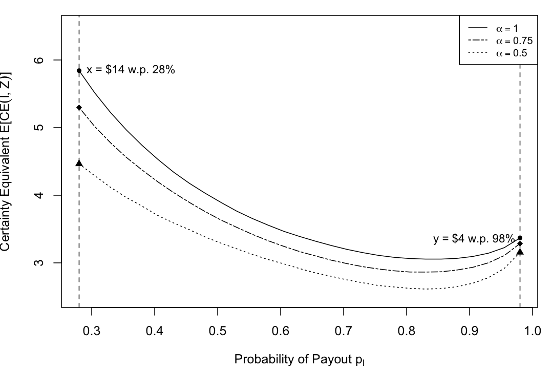
Figure 6: Simulated average certainty equivalents $E[CE(l,Z)]$ for simple lotteries $l=(w_{l},p_{l})$ with expected value equal to that of $x=(14,0.28)$ as a function of $p_{l}$. In these simulations, $Z$ is adapted to $l$, and we set $|Z|=15$. $\tau_{xy}$ has a CDF-complexity representation parameterized by $u(w)=w^{\alpha}$ and $H(r)=(\Phi^{-1}(G(r)))^{2}$, for $G$ given by (1) with $\kappa=0,\gamma=0.75$. Priors are distributed $Q\sim U[0,1]$.

First consider the certainty equivalents of $x$ and $y$, which correspond to the intersection of each curve with the vertical dashed lines in Figure 6: although $y$ is weakly preferred to $x$ since the DM is risk-averse, the model predicts that $x$ is valued higher than $y$ on average. The intuition is as follows: since the low-probability lottery $x$ is dissimilar to and therefore difficult to compare to money, its valuation is pulled to the midpoint of the undominated range of prices $[0,w_{x}]$, and so the valuation of $x$ is inflated. On the other hand, since the high-probability lottery is easier to compare to money its valuation will exhibit a lower level of bias and if anything will be distorted downwards towards the midpoint of undominated prices $[0,w_{y}]$. As such, our model rationalizes preference reversals, where $\rho(y,x)\geq 1/2$ and yet $E[CE(x,Z)]>E[CE(y,Z)]$.

The entirety of the figure traces our model’s predictions for preference reversals in general: for $x^{\prime}$ with a modest payoff probability and $y^{\prime}$ with a high payoff probability, we will have $E[CE(x^{\prime},Z)]>E[CE(y^{\prime},Z)]$ for with a high payoff probability — despite the fact that $y^{\prime}$ is in truth preferred to $x^{\prime}$, and so $\rho(y^{\prime},x^{\prime})\geq 1/2$.

In our model, preference reversals result from the differential ease of comparing lotteries to money. This suggests that one may be able to eliminate or even reverse the direction of these effects by changing the numeraire: the currency against which the lotteries are valued.

Example 3.

(Reversals with probability equivalents). For instance, consider the same lotteries $x$ and $y$ from Example 2, and imagine that instead of valuing $x$ and $y$ in terms of money, the DM is asked to assess the probability-equivalents of the lotteries: the probability $p$ that makes the lottery $z=(\$15,p)$ indifferent to $x$ and $y$.

$$x:\quad\$14\text{ with 28\%}$$

$$y:\quad\$4\text{ with 98\%}$$

Whereas $y$ was easier to compare to money, $x$ is now easier to compare to the new numeraire. Our model predicts that this change in numeraire reverses the distortion in the valuation of $x$ and $y$.

Formally, rather than valuing a simple lottery $l=(w_{l},p_{l})$ against a price list, the decision-maker now values $l$ against a probability list $Z=(z_{1},...,z_{k})$, where each $z^{k}=(15,p_{k})$. Analogous to the restriction made in Example 2, call a probability list $Z$ adapted to $l$ if $p_{k}-p_{k+1}$ is constant in $k$ and $p_{1}=p_{l}$, $p_{n}=0$. Analogous to before, let $PE(l,Z)=1/2[p_{R(l,Z)-1}+p_{R(l,Z)}]$ denote the distribution over the DM’s probability equivalents, obtained from assigning each switching point to a probability equivalent at the midpoint of the adjacent probabilities.

Figure 7 plots the expected probability equivalents $E[PE(l,Z)]$, simulated from our model with CRRA preferences, for the same set of lotteries as in Figure 6: simple lotteries $l$ with the same expected value as $x$ and $y$,

Consider the probability equivalents of $x$ and $y$, given by the intersection of each curve with the vertical dashed lines in Figure 7. Whereas $x$ was valued higher than $y$ on average when valued in terms of certainty equivalents, our model predicts that the distortion in valuations reverses when the lotteries are valued in terms of probability equivalents: we have $E[PE(y,Z)]>E[PE(x,Z)]$. Intuitively, $y$ is hard to compare to the $z_{k}$, so its valuation is compressed upward towards the middle of the range of undominated probabilities $[0,p_{y}]$, whereas $x$ is easy to compare to $z_{k}$, and so its valuation will be close to the truth.

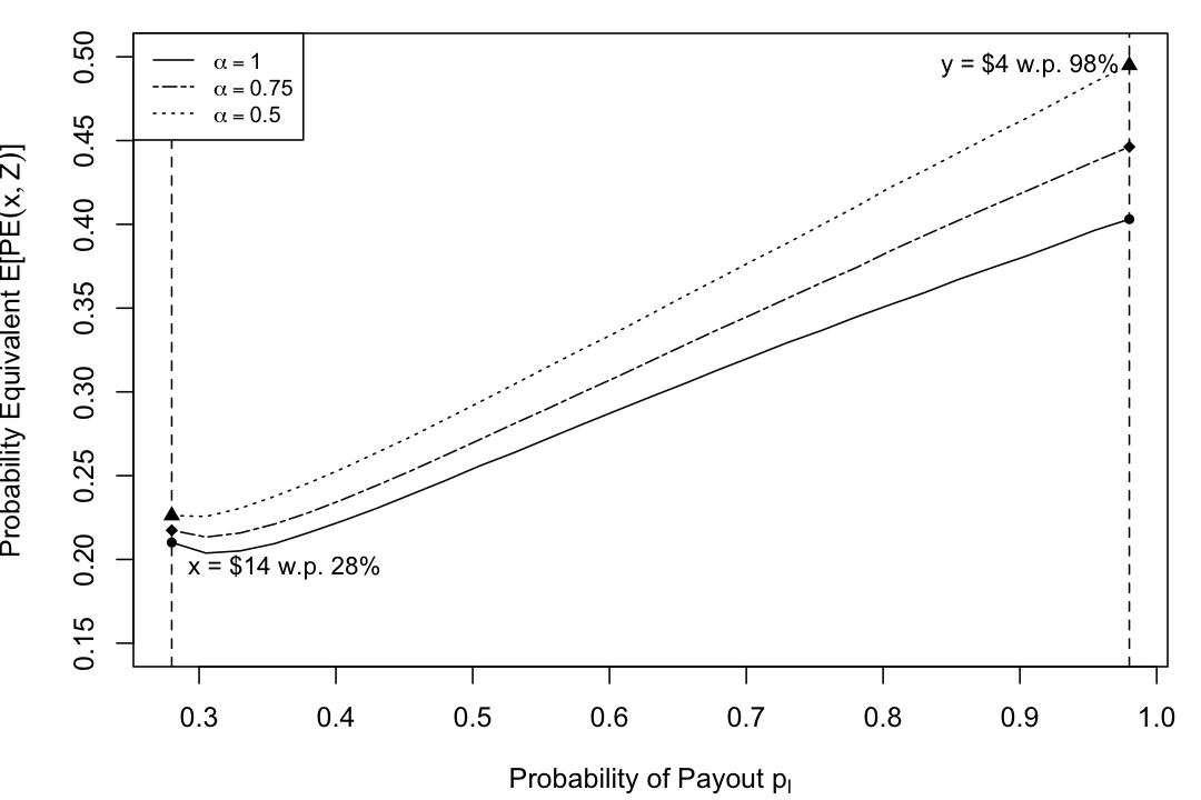
Figure 7: Simulated average probability equivalents $E[PE(l,Z)]$ for simple lotteries $l=(w_{l},p_{l})$ with expected value equal to that of $x=(14,0.28)$ as a function of $p_{l}$. In these simulations, $Z$ is adapted to $l$ and we set $|Z|=15$. $\tau_{xy}$ has a CDF-complexity representation parameterized by $u(w)=w^{\alpha}$ and $H(r)=(\Phi^{-1}(G(r)))^{2}$, for $G$ given by (1) with $\kappa=0,\gamma=0.75$. Priors are distributed $Q\sim U[0,1]$.

Importantly, even though valuation using probability equivalents reverses the distortions responsible for preference reversals in this example, our model does not predict that valuations using probability equivalents are systematically more accurate than certainty equivalents. To see this, focus on the predictions of the model in the case of risk neutral preferences. Here, both methods of valuation are subject to bias: $x$ and $y$ are indifferent in truth, and yet we have $E[CE(x,Z)]>E[CE(y,Z)]$ and $E[PE(x,Z)]<E[PE(y,Z)]$.

Intertemporal Choice. The logic above, which shows the differential ease of comparing options to the numeraire can rationalize preference reversals, is not limited to risky choice.

Consider the following example of a preference reversal in intertemporal choice, documented by Tversky et al., (1990) using choice vignettes:

$$x:\quad\$3550\text{ in 10 years}$$

$$y:\quad\$1600\text{ in 1.5 years}$$

The authors find that in direct choice, a majority of subjects choose the earlier payment $y$, but that when tasked with valuing the options in terms of money today, most subjects value the more delayed payment $x$ higher than $y$.

In Appendix B.5, we show how our model applied to the intertemporal domain rationalizes such preference reversals as the consequence of $y$ being more similar to and therefore easier to compare to money today than $x$.

4.3.3 Biases in Valuation of Risk and Time

The pattern of biased valuation presented in Figure 6 also generates apparent probability-weighting in certainty equivalents. To see why this is true, suppose we have a risk-neutral agent and we elicit certainty equivalents on simple lotteries to measure the agent’s probability weighting function. Previously, we argued that low-probability lotteries will be over-valued and high-probability lotteries will be under-valued. Thus, if we estimated the agent’s probability weighting function based on her valuations, we would conclude the agent is overweighting small probabilities and underweighting large probabilities.

To illustrate this, consider the standard paradigm used to estimate the probability weighting function, in which the DM provides certainty equivalents of simple lotteries $l=(\overline{w},p_{l})$. Figure 8 plots the predicted normalized certainty equivalents $E[CE(l,Z)]/\overline{w}$ as a function of $p_{l}$ for a DM with CRRA preferences. The weights implied by these certainty equivalents reproduce the familiar inverse S-shaped pattern of probability weighting.

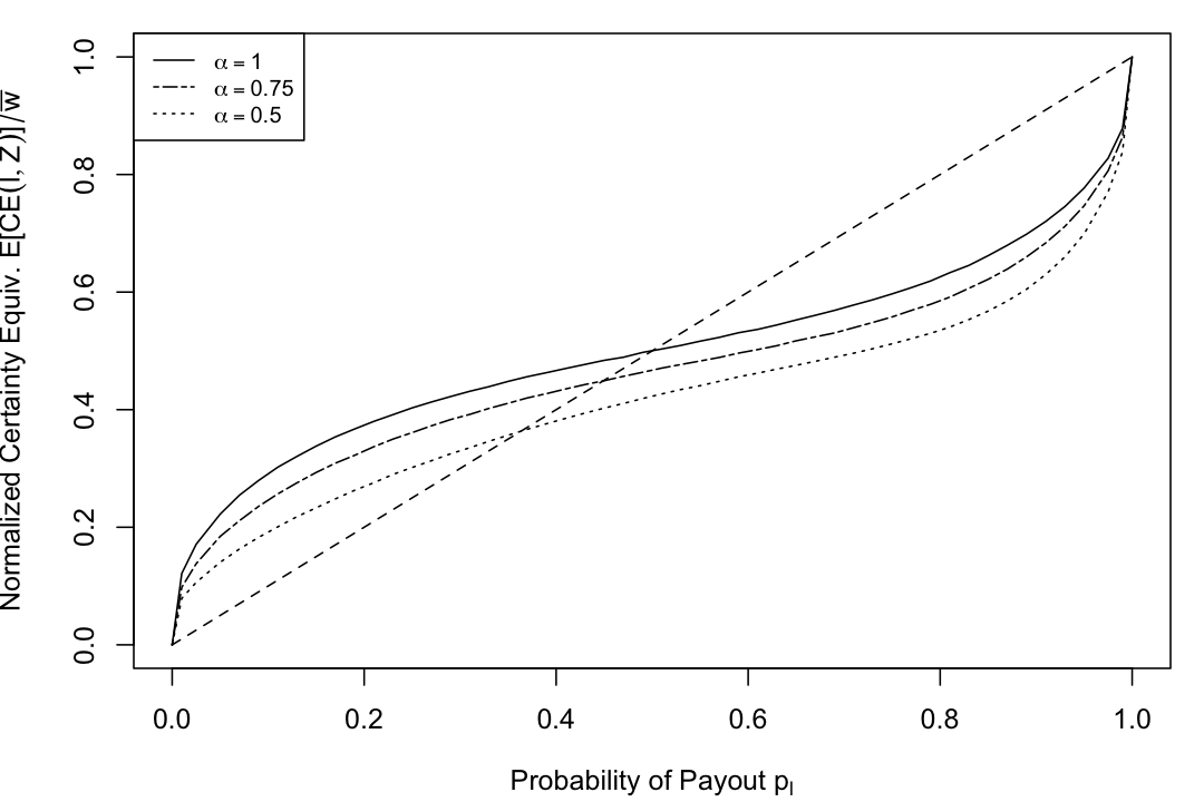
Figure 8: Simulated normalized average certainty equivalents $E[CE(l,Z)]/\overline{w}$ for simple lotteries $l=(\overline{w},p_{l})$ as a function of $p_{l}$. In these simulations, $Z$ is adapted to $l$ and we set $|Z|=15$. $\tau_{xy}$ has a CDF-complexity representation parameterized by $u(w)=w^{\alpha}$ and $H(r)=(\Phi^{-1}(G(r)))^{2}$, for $G$ given by (1) with $\kappa=0,\gamma=0.75$. Priors are distributed $Q\sim U[0,1]$.

In our model, this apparent probability weighting does not reflect a true preference, but instead a bias resulting from the complexity of comparing a lottery to a price list. This is important for two reasons. First, we do not predict probability weighting in binary choice, which is consistent with evidence that the inverse S-shaped probability weighting function is far more prominent in valuation tasks than in direct choice (Harbaugh et al.,, 2010; Bouchouicha et al.,, 2023). Second, we predict that these seeming patterns of probability weighting will be highly sensitive to the units against which the lotteries are valued. In particular, we predict that it is possible to reverse the pattern of apparent probability-weighting with an appropriate choice of price list currency.

Consider an alternative paradigm for estimating the probability weighting function, in which the DM provides probability equivalents of a certain payout: the probability $p$ that makes the lottery $z=(\overline{w},p)$ indifferent to a certain payment $c=(w_{c},1)$. Tracing out the probability equivalents $p$ as a function of the normalized certain payments $w_{c}/\overline{w}$ should — assuming no complexity-driven distortions — recover the same preference information as the certainty equivalents discussed above. Figure 9 plots the predicted relationship between the certain payment amount $w_{c}/\overline{w}$ (y-axis) and the associated probability equivalent $E[PE(c,Z)]$ (x-axis), in which the certain payment $c=(w_{c},1)$ is valued against a probability list $Z=(z^{1},...,z^{k})$, for $z^{k}=(\overline{w},p_{k})$. Here we see a reversal of the inverse S-shaped pattern: the difficulty of comparing sure payments against the numeraire good causes probability equivalents to be compressed towards the middle of the price list, generating apparent underweighting of small probabilities and overweighting over large probabilities. This is an empirical prediction which could be tested experimentally.

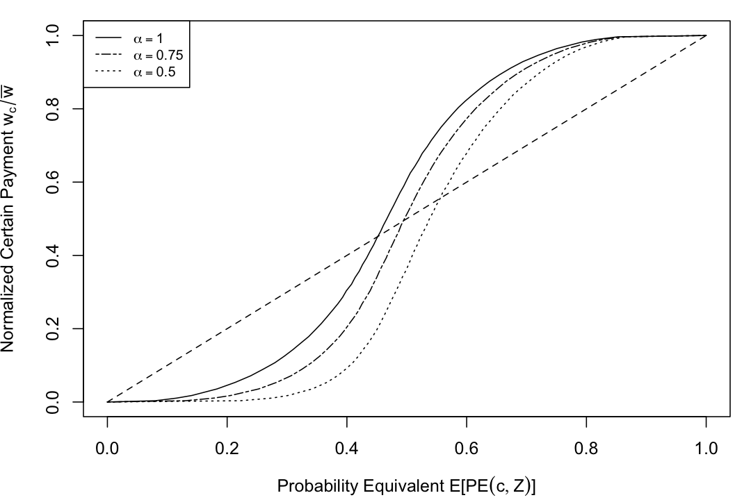
Figure 9: Relationship between simulated average probability equivalents $E[PE(c,Z)]$ for a certain payment $c=(w_{c},p_{l})$ and the normalized payment amount $w_{c}/\overline{w}$. In these simulations, $Z$ is adapted to $l$ and we set $|Z|=15$. $\tau_{xy}$ has a CDF-complexity representation parameterized by $u(w)=w^{\alpha}$ and $H(r)=(\Phi^{-1}(G(r)))^{2}$, for $G$ given by (1) with $\kappa=0,\gamma=0.75$. Priors are distributed $Q\sim U[0,1]$.

Importantly, we do not claim that distorted probability weighting functions do not exist – instead, our model offers a potential explanation for why canonical valuation tasks over simple lotteries may overstate the degree of any true probability weighting.

We can consider a similar exercise in the context of valuing intertemporal payment streams, where we see that complexity-driven noise generates apparent hyperbolic discounting even in the absence of hyperbolicity in preferences. We work out this exercise in full in Appendix B.6, but the logic is much the same as probability-weighting. In traditional price-list elicitations, payments dated close to the present will be undervalued, as valuations are pulled down towards the center of the price list; and payments further in the future will be overvalued, as valuations are pulled up towards the center of the price list. This produces a pattern of complexity-driven hyperbolic discounting, which is consistent with evidence from (Enke et al.,, 2023). We further predict that this pattern persists when front-end delays are incorporated, since the apparent hyperbolicity predicted by our model is not driven by a preference for the present. This is also supported by evidence from (Enke et al.,, 2023).

Importantly, our model predicts that these distortions are not generic, but instead arise specifically from the difficulty of comparing delayed payments to the numeraire good of money today. As with lotteries, our model predicts that we can reverse the pattern of hyperbolic discounting by instead eliciting valuations in time-equivalents rather than money-equivalents, as discussed in B.6. Once again, we do not claim that real present-biased preferences do not exist; rather, our model suggests a mechanism for why canonical valuation tasks may overstate the true degree of hyperbolic discounting.

5 Conclusion

This paper presents a new theory of comparison-based complexity in multiattribute, lottery, and intertemporal choice, in which comparisons are easier when two options are more similar along their features (holding value difference fixed); and easiest when two options have a dominance relationship. We provide experimental evidence that our measures of comparison complexity predict choice errors, choice inconsistency, and cognitive uncertainty. Finally, we show how comparison complexity can generate systematically biased choices and valuations. In particular, our choice model rationalizes familiar context effects like the decoy and asymmetric dominance; classic preference reversals; and probability weighting and hyperbolic discounting in risk and time respectively. Furthermore, our model predicts that it is possible to reverse the standard patterns of probability weighting and hyperbolic discounting, depending on how the researcher chooses the currency against which options are valued.

Appendix A Appendix: Tables and Figures

Table 2: Complexity Responses vs. $L_{1}$ Ratio

	Dependent Variable: Error Rate			Dependent Variable: Inconsistency Rate			Dependent Variable: CU
	(1)	(2)		(3)	(4)		(5)	(6)
$L_{1}$ Ratio	$-0.26^{***}$	$-0.26^{***}$		$-0.19^{***}$	$-0.19^{***}$		$-0.12^{***}$	$-0.12^{***}$
	$(0.02)$	$(0.02)$		$(0.02)$	$(0.02)$		$(0.01)$	$(0.01)$
Global Value Difference		$0.00$			$-0.01$			$-0.00$
		$(0.00)$			$(0.01)$			$(0.00)$
(Intercept)	$0.32^{***}$	$0.32^{***}$		$0.26^{***}$	$0.28^{***}$		$0.25^{***}$	$0.27^{***}$
	$(0.01)$	$(0.02)$		$(0.01)$	$(0.03)$		$(0.00)$	$(0.01)$
R2	$0.32$	$0.32$		$0.03$	$0.03$		$0.30$	$0.31$
Adj. R2	$0.32$	$0.32$		$0.03$	$0.03$		$0.30$	$0.31$
Num. obs.	$662$	$662$		$4880$	$4880$		$662$	$662$
OLS Estimates. Standard errors (in parentheses) are robust. “$L_{1}$ Ratio" and “Global Value Difference" are the $L_{1}$ ratio and the monetary value difference for each choice problem. ${}^{***}p<0.001$; ${}^{**}p<0.01$; ${}^{*}p<0.05$.

Table 3: Complexity Responses vs. $L_{1}$ Ratio, No Calculator Users

	Dependent Variable: Error Rate			Dependent Variable: Inconsistency Rate			Dependent Variable: CU
	(1)	(2)		(3)	(4)		(5)	(6)
$L_{1}$ Ratio	$-0.30^{***}$	$-0.29^{***}$		$-0.20^{***}$	$-0.20^{***}$		$-0.12^{***}$	$-0.12^{***}$
	$(0.02)$	$(0.02)$		$(0.02)$	$(0.02)$		$(0.01)$	$(0.01)$
Global Value Difference		$-0.00$			$-0.01$			$-0.00^{*}$
		$(0.00)$			$(0.01)$			$(0.00)$
(Intercept)	$0.36^{***}$	$0.36^{***}$		$0.28^{***}$	$0.32^{***}$		$0.26^{***}$	$0.28^{***}$
	$(0.01)$	$(0.03)$		$(0.01)$	$(0.03)$		$(0.01)$	$(0.01)$
R2	$0.32$	$0.32$		$0.03$	$0.03$		$0.30$	$0.30$
Adj. R2	$0.32$	$0.32$		$0.03$	$0.03$		$0.30$	$0.30$
Num. obs.	$662$	$662$		$4020$	$4020$		$662$	$662$
OLS Estimates. Standard errors (in parentheses) are robust. “$L_{1}$ Ratio" and “Global Value Difference" are the $L_{1}$ ratio and the monetary value difference for each choice problem. ${}^{***}p<0.001$; ${}^{**}p<0.01$; ${}^{*}p<0.05$.

Table 4: Structural Estimates: Multiattribute Choice

		BGS	Focus	RT	$L_{1}$-C, 2P	$L_{1}$-C, 3P
Parameter Estimates
$\delta$		1
$\theta$			0
$\omega$				0.84
$\xi$				1.62
$\kappa$					0.09	0.04
$\gamma$					2.36	0.86
$\psi$						0.55
$\eta$		0.37	0.37	1.54
$R^{2}$		0.001	0.001	0.345	0.289	0.32
“BGS", “Focus", and “RT" refer to the Salience, Focusing, and Relative Thinking models described in Appendix E.1. “$L_{1}$-C, 2P" and “$L_{1}$-C, 3P" refer to the 2 and 3 parameter $L_{1}$-Complexity models described in Appendix E.1.

Table 5: Predicted vs. Actual Choice Rates, Multiattribute Choice

	Dependent Variable: Choice Rates
	(1)	(2)	(3)	(4)	(5)
BRS Choice Rates	$0.82^{***}$		$0.58^{***}$		$0.54^{***}$
	$(0.05)$		$(0.07)$		$(0.07)$
$L_{1}$ Choice Rates, 2 param.		$0.81^{***}$	$0.41^{***}$
		$(0.06)$	$(0.07)$
$L_{1}$ Choice Rates, 3 param.				$1.00^{***}$	$0.57^{***}$
				$(0.06)$	$(0.07)$
(Intercept)	$0.16^{***}$	$0.17^{**}$	$0.01$	$0.00$	$-0.09$
	$(0.05)$	$(0.05)$	$(0.05)$	$(0.06)$	$(0.05)$
R2	$0.35$	$0.29$	$0.39$	$0.32$	$0.41$
Adj. R2	$0.34$	$0.29$	$0.39$	$0.32$	$0.41$
Num. obs.	$662$	$662$	$662$	$662$	$662$
OLS Estimates. Standard errors (in parentheses) are robust. “BRS Choice Rates", “$L_{1}$ Choice Rates, 2 param.", and “$L_{1}$ Choice Rates, 3 param." refer to the predicted choice rates of the structurally estimated relative thinking model and $L_{1}$ models, respectively. ${}^{***}p<0.001$; ${}^{**}p<0.01$; ${}^{*}p<0.05$.

Table 6: Complexity Responses vs. CPF Ratio

	Dependent Variable: Error Rate			Dependent Variable: Inconsistency Rate			Dependent Variable: CU
	(1)	(2)		(3)	(4)		(5)	(6)
Global CPF Ratio	$-0.51^{***}$	$-0.51^{***}$		$-0.20^{***}$	$-0.17^{***}$		$-0.07^{***}$	$-0.07^{***}$
	$(0.01)$	$(0.01)$		$(0.01)$	$(0.01)$		$(0.00)$	$(0.00)$
Global Value Difference		$-0.00$			$-0.01^{***}$			$-0.00$
		$(0.00)$			$(0.00)$			$(0.00)$
(Intercept)	$0.55^{***}$	$0.55^{***}$		$0.27^{***}$	$0.28^{***}$		$0.15^{***}$	$0.15^{***}$
	$(0.01)$	$(0.01)$		$(0.01)$	$(0.01)$		$(0.00)$	$(0.00)$
R2	$0.60$	$0.60$		$0.02$	$0.03$		$0.22$	$0.23$
Adj. R2	$0.59$	$0.59$		$0.02$	$0.03$		$0.22$	$0.22$
Num. obs.	$1100$	$1100$		$16580$	$16580$		$1100$	$1100$
OLS estimates. Standard errors (in parentheses) are robust. “Global CPF" Ratio" and “Global Value Difference" are the representative-agent CPF ratio and value difference for each choice problem, computed using the value of $\delta$ estimated in the Exponential Discounting model described in Appendix E.2. ${}^{***}p<0.001$; ${}^{**}p<0.01$; ${}^{*}p<0.05$.

Table 7: Individual-Level Error Rates vs. CPF Ratio

	Dependent Variable: Binary Error (Indiv. $\hat{\delta}$)
	(1)	(2)	(3)	(4)
Global CPF Ratio	$-0.18^{***}$	$-0.17^{***}$
	$(0.01)$	$(0.01)$
Indiv. CPF Ratio			$-0.38^{***}$	$-0.34^{***}$
			$(0.01)$	$(0.01)$
Indiv. Value Difference		$-0.01^{***}$		$-0.01^{***}$
		$(0.00)$		$(0.00)$
(Intercept)	$0.25^{***}$	$0.31^{***}$	$0.40^{***}$	$0.40^{***}$
	$(0.00)$	$(0.01)$	$(0.01)$	$(0.01)$
R2	$0.02$	$0.06$	$0.10$	$0.11$
Adj. R2	$0.02$	$0.06$	$0.10$	$0.11$
Num. obs.	$41450$	$41450$	$41450$	$41450$
OLS estimates. Standard errors (in parentheses) are robust. “Global CPF" Ratio" is the representative-agent CPF ratio for each subject-choice problem, computed using the value of $\delta$ estimated in the Exponential Discounting model described in Appendix E.2. “Indiv. CPF" Ratio" and “Indiv. Value Difference" are the individual-level CPF ratio and value difference for each subject-choice problem, computed using the individual-level $\delta_{i}$ estimates under the same model. ${}^{***}p<0.001$; ${}^{**}p<0.01$; ${}^{*}p<0.05$.

Table 8: Structural Estimates: Intertemporal Choice

		EDU	HDU	CPF-C
Parameter Estimates
$\delta$		0.95		0.96
$\upsilon$			0.16
$\zeta$			0.12
$\kappa$				0.03
$\gamma$				0.85
$\eta$		0.35	0.43
$R^{2}$		0.75	0.78	0.88
“EDU", “HDU", and “CPF-C" refer to the Exponential Discounting, Hyperbolic Discounting, and CPF Complexity models described in Appendix E.2. For these estimates, each time period is 24 days.

Table 9: Complexity Responses vs. CDF Ratio

	Dependent Variable: Error Rate			Dependent Variable: Inconsistency Rate			Dependent Variable: CU
	(1)	(2)		(3)	(4)		(5)	(6)
Global CDF Ratio	$-0.32^{***}$	$-0.28^{***}$		$-0.10^{***}$	$-0.11^{***}$		$-0.19^{***}$	$-0.21^{***}$
	$(0.00)$	$(0.00)$		$(0.00)$	$(0.00)$		$(0.01)$	$(0.01)$
Global Value Difference		$-0.01^{***}$			$0.00^{***}$			$0.01^{***}$
		$(0.00)$			$(0.00)$			$(0.00)$
(Intercept)	$0.48^{***}$	$0.51^{***}$		$0.28^{***}$	$0.28^{***}$		$0.25^{***}$	$0.22^{***}$
	$(0.00)$	$(0.00)$		$(0.00)$	$(0.00)$		$(0.01)$	$(0.01)$
R2	$0.45$	$0.47$		$0.10$	$0.11$		$0.31$	$0.35$
Adj. R2	$0.45$	$0.47$		$0.10$	$0.11$		$0.31$	$0.35$
Num. obs.	$10923$	$10923$		$10423$	$10423$		$500$	$500$
OLS estimates. Standard errors (in parentheses) are robust. “Global CDF" Ratio" and “Global Value Difference" are the representative-agent CDF ratio and value difference for each choice problem, computed using the value of $\alpha$ estimated in the Expected Utility model described in Appendix E.3. ${}^{***}p<0.001$; ${}^{**}p<0.01$; ${}^{*}p<0.05$.

Table 10: Individual-Level Error Rates vs. CDF Ratio

	Dependent Variable: Binary Error (Indiv. $\hat{\alpha}$)
	(1)	(2)	(3)	(4)
Global CDF Ratio	$-0.43^{***}$	$-0.40^{***}$
	$(0.01)$	$(0.01)$
Indiv. CDF Ratio			$-0.37^{***}$	$-0.35^{***}$
			$(0.01)$	$(0.01)$
Indiv. Value Difference		$0.00^{***}$		$0.00^{***}$
		$(0.00)$		$(0.00)$
(Intercept)	$0.59^{***}$	$0.53^{***}$	$0.57^{***}$	$0.51^{***}$
	$(0.01)$	$(0.01)$	$(0.01)$	$(0.01)$
R2	$0.08$	$0.09$	$0.06$	$0.08$
Adj. R2	$0.08$	$0.09$	$0.06$	$0.08$
Num. obs.	$12500$	$12500$	$12500$	$12500$
OLS estimates. Standard errors (in parentheses) are robust. “Global CDF" Ratio" is the representative-agent CDF ratio for each subject-choice problem, computed using the value of $\alpha$ estimated in the Expected Utility model described in Appendix E.3. “Indiv. CDF" Ratio" and “Indiv. Value Difference" are the individual-level CPF ratio and value difference for each subject-choice problem, computed using the individual-level $\alpha_{i}$ estimates under the same model. ${}^{***}p<0.001$; ${}^{**}p<0.01$; ${}^{*}p<0.05$.

Table 11: Structural Estimates: Lottery Choice

		EU	RDEU	CPT	EV CDF-C	EU CDF-C
Parameter Estimates
$\alpha$		0.85	0.83	0.75		0.59
$\beta$			0.79	0.78
$\lambda$				0.79
$\chi$				1.06
$\nu$				0.83
$\kappa$					0.15	0.15
$\gamma$					0.77	0.71
$\eta$		0.22	0.24	0.33
$R^{2}$		0.55	0.56	0.59	0.66	0.73
“EU", “RDEU", and “CPT" refer to the Expected Utility, Reference-Dependent Expected Utility, and Cumulative Prospect Theory models described in Appendix E.3. “EV CDF-C" and “EU CDF-C" refer to the risk-neutral and expected utility CDF complexity models described in Appendix E.3.

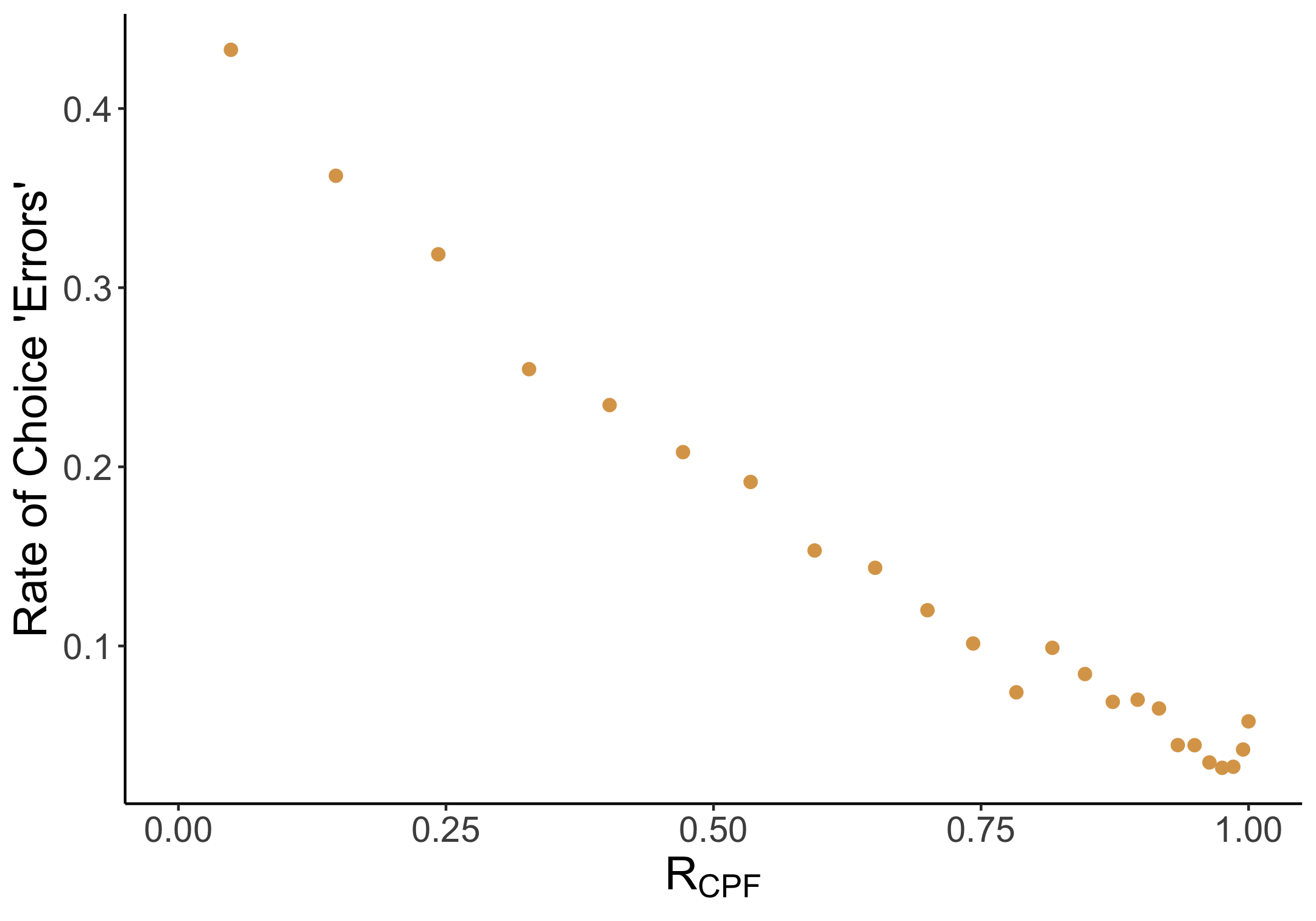
Figure 10: Binscatter of individual-level error dummies against individual-level CPF ratios. A choice is coded as an “error” if the individual chooses the lower-value option, according to the best-fit discount function estimated on their 50 experimental choices. We use the same 2-parameter structural model as in estimating global temporal preferences, which features exponential discounting and logit noise. The estimating equation is provided in Appendix E.2

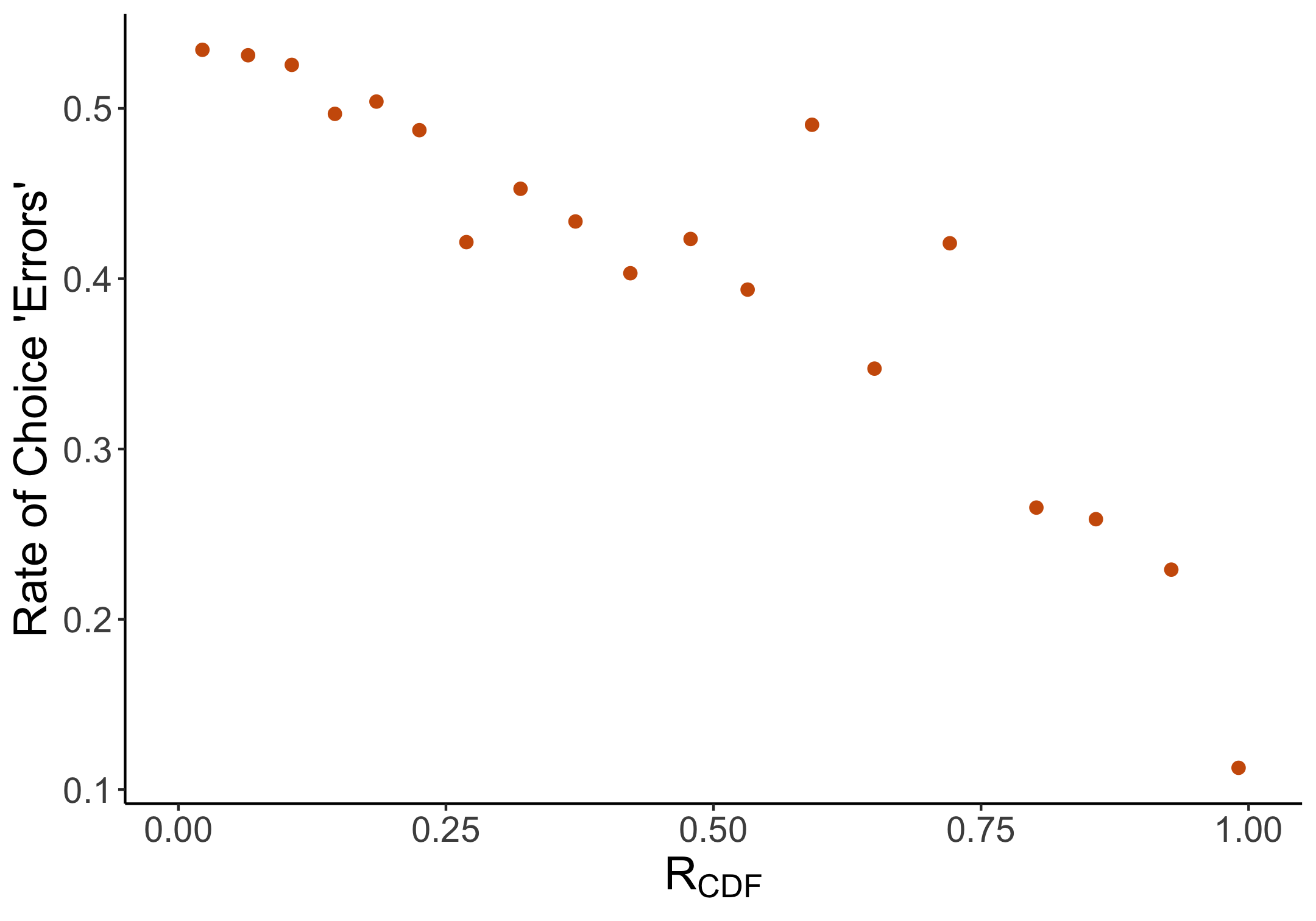
Figure 11: Binscatter of individual-level error dummies against individual-level CDF ratios. Analogously to time, a choice is coded as an “error” if the individual chooses the lower-value option, according to the utility function estimated on their 50 experimental choices. We use a 2-parameter structural model of risk preferences, which features symmetric CRRA utility and logit noise. The estimating equation is provided in Appendix E.3; we employ the parameter restriction $\alpha_{i}\geq 0.35$ in our estimations.

Appendix B Appendix: Additional Theoretical Results

B.1 Axiomatic Characterizations

B.1.1 Linear Multiattribute Choice

We state our characterization theorem in the case where $n\geq 2$. The $n=2$ case requires an additional axiom. Let $x_{\{k\}}=x_{\{k\}}\vec{0}$.

1. Exchangeability: If $\rho(x_{\{i\}},x_{\{j\}}^{\prime})=1/2$ and $\rho(x_{\{j\}},x_{\{i\}}^{\prime})=1/2$, with $x_{k}=x^{\prime}_{k}=0$ for all $k\neq i,j$, then $\rho(x,0)=\rho(x^{\prime},0)$.

Exchangeability states that swapping attribute labels (adjusting for attribute weights) will not affect choice, and arises from the fact in our theory, the similarity in the denominator is defined over the same value-transformed attributes that govern preferences.

Theorem 2.

Suppose that all attributes are non-null. A binary choice rule $\rho$ satisfies M1–M6 iff it has an $L_{1}$-complexity representation $(G,\beta)$. If $n>2$, $\rho$ satisfies M1–M5 iff it has an $L_{1}$ complexity representation $(G,\beta)$. Furthermore, if $\rho$ also has an $L_{1}$-complexity representation $(G^{\prime},\beta^{\prime})$ then $G^{\prime}=G$ and there exists $C>0$ such that $\beta^{\prime}=C\beta$.

B.1.2 Additively Separable Multiattribute Choice

We consider an extended multiattribute domain where each option in $X\equiv X_{1}\times X_{2}\times...\times X_{n}$ is defined on $n$ attribute dimensions, where each $X_{i}$ is a connected and separable topological space. Preferences are additively separable in each attribute, where the value of each $x$ is given by $U(x)=\sum_{k}u_{k}(x_{k})$ for $u_{k}$ continuous. Say that $u_{k}$ is non-trivial if there exist $x_{k},x^{\prime}_{k}\in X_{k}$ such that $u_{k}(x_{k})\neq u_{k}(x^{\prime}_{k})$. We propose that the ease of comparison in this domain is governed by the following representation:

Definition 5.

$\tau_{xy}$ has an additively separable $L_{1}$-complexity representation if there exist continuous, non-trivial $u_{i}:X_{i}\to\mathbb{R}$ such that for $U(x)=\sum_{k}u_{k}(x_{k})$ and $d_{L1}(x,y)=\sum_{k}|u_{k}(x_{k})-u_{k}(y_{k})|$, whenever $d_{L1}(x,y)\neq 0$

$$\tau_{xy}=H\left(\frac{|U(x)-U(y)|}{d_{L1}(x,y)}\right)$$

for $H$ continuous, increasing with $H(0)=0$, and $\tau_{xy}=0$ otherwise. Similarly, a binary choice rule $\rho$ has an additively separable $L_{1}$-complexity representation if there exist continuous, non-trivial $u_{i}:X_{i}\to\mathbb{R}$ such that whenever $d_{L1}(x,y)\neq 0$,

$$\rho(x,y)=G\left(\frac{U(x)-U(y)}{d_{L1}(x,y)}\right).$$

for $G$ continuous, strictly increasing, and $\rho(x,y)=1/2$ otherwise.

Note that this representation for $\tau_{xy}$ satisfies the same principles of similarity, dominance, and simplification as the linear representation introduced in Section 2.1, and the corresponding representation for $\rho(x,y)$ satisfies axioms M1 and M3–M5. We provide an axiomatic characterization for this representation, in which Linearity is relaxed and replaced with two axioms.

First some definitions. For $E\subseteq I$, let $x_{E}y$ denote the option that replaces the value of option $y$ along attributes $k\in E$ with $x_{k}$. Say that comparisons $(x,y),(w,z)\in\mathcal{D}$, are congruent if for all $i\in I$, $\rho(x_{\{i\}}y,y)\geq 1/2$ and $\rho(w_{\{i\}}z,z)\geq 1/2$ or $\rho(x_{\{i\}}y,y)\leq 1/2$ and $\rho(w_{\{i\}}z,z)\leq 1/2$. That is, if $(x,y)$ and $(w,z)$ are congruent, the advantages and disadvantages in the two comparisons are located in the same attributes.

1. Separability: $\rho(x_{E}z,y_{E}z)=\rho(x_{E}z^{\prime},y_{E}z^{\prime})$ for all $x,y,z,z^{\prime}\in X$, $E\subseteq I$.

2. Tradeoff Congruence. Suppose that $(x,y)$ is congruent to $(y,z)$, and $\rho(x,y),\rho(y,z)\geq 1/2$. Then $\rho(x,z)\leq\max\{\rho(x,y),\rho(y,z)\}$.

Separability is the stochastic analog of the familiar coordinate independence axiom in deterministic choice, which says that $x_{E}z\succeq y_{E}z\implies x_{E}z^{\prime}\succeq y_{E}z^{\prime}$ for all $E\subseteq I$, $x,y,z,z^{\prime}\in X$. The interpretation of Tradeoff Congruence is as follows: consider the attribute-wise tradeoffs involved in comparing $z$ to $y$ and $x$ to $y$, where $x$ is in fact better than $y$, and $y$ is better than $z$. If replacing $y$ with $x$ in the first comparison and replacing $y$ with $z$ in the second only increases the magnitude of these tradeoffs – i.e. if $(x,y)$ and $(y,z)$ are congruent – then $(x,z)$ cannot be an easier comparison than both of the intermediate comparisons $(x,y)$ and $(y,z)$. Intuitively, neither of these replacements reduce the size of the tradeoffs the DM must contend with, and so as revealed by choice probabilities, the DM cannot find the comparison $(x,z)$ easier than both $(x,y)$ and $(y,z)$.

The following result states that Continuity, Moderate Transitivity, Dominance, Simplification, Separability, and Tradeoff Congruence characterize the additively separable representation, and that its primitives are identified from choice data.

Theorem 3.

Suppose that $n>2$ and that all attributes are non-null. Then a binary choice rule $\rho$ satisfies M1,M3–M5, M7–M8 if and only if it has an additively separable $L_{1}$-complexity representation. Morever, suppose that at least two attributes are non-null. If $\rho$ has additively separable $L_{1}$ complexity representations $((u_{i})_{i=1}^{n},G)$ and $((u^{\prime}_{i})_{i=1}^{n},G^{\prime})$, then there exists $C>0$, $b_{i}\in\mathbb{R}$ such that $u_{i}^{\prime}=Cu_{i}+b_{i}$ for all $i$, and $G^{\prime}=G$.

B.1.3 Lottery Choice

Consider the lottery choice domain, where $X$ is the set of finite state lotteries over $\mathbb{R}$. Note that the CDF-complexity representation for $\tau_{xy}$ implies the following binary choice representation:

Definition 6.

A binary choice rule $\rho$ has a CDF-Complexity representation if there exists $u:\mathbb{R}\to\mathbb{R}$ strictly increasing such that

$$\rho(x,y)=G\left(\frac{EU(x)-EU(y)}{d_{CDF}(x,y)}\right)$$

for $G$ continuous, strictly increasing.

Let $\geq$ denote the partial order $X$ corresponding to first-order stochastic dominance. Let $S_{x}=\{w\in\mathbb{R}:f_{x}(w)>0\}$ denote the support of lottery $x$. Consider the following axioms:

1. Continuity: $\rho(x,y)$ is continuous on its domain.

2. Independence: $\rho(x,y)=\rho(\lambda x+(1-\lambda)z,\lambda y+(1-\lambda)z)$ for $\lambda\in(0,1)$.

3. Moderate Stochastic Transitivity: If $\rho(x,y)\geq 1/2$, $\rho(y,z)\geq 1/2$, then either $\rho(x,z)>\min\{\rho(x,y),\rho(y,z)\}$ or $\rho(x,z)=\rho(x,y)=\rho(y,z)$.

4. Dominance: $x\geq y$, then $\rho(x,y)\geq\rho(w,z)$ for any $w,z\in L(S)$, where the inequality is strict if $w\not\geq z$.

5. Simplification. For any $x,y\in X$ and $w^{*}\in S_{x}\cup S_{y}$, consider $x^{\prime}$ with support in $S_{x}\cup S_{y}$ satisfying $F_{x^{\prime}}(w^{*})=F_{y}(w^{*})$, and $F_{x^{\prime}}(w)\neq F_{x}(w)$ for at most one $w\in S_{x}\cup S_{y}/\{w^{*}\}$. If $\rho(x,y)\geq 1/2$ and $\rho(x^{\prime},x)=1/2$, then $\rho(x^{\prime},y)\geq\rho(x,y)$.

Axioms L1–L4 are the direct analogs of M1–M4 in the characterization of $L_{1}$ complexity. Axiom L5 says that concentrating value differences between lotteries in the same region of the distribution of the lotteries makes them easier to compare, and is an analog of the Simplification property (Axiom M5) for $L_{1}$ complexity. Axioms L1–L5 exhaust the behavioral content of CDF complexity.

Theorem 4.

A binary choice rule $\rho$ satisfies L1-L5 if and only if it has a CDF-Complexity representation $(G,u)$. Moreover, if $(G^{\prime},u^{\prime})$ also represents $\rho$, then $G^{\prime}=G$ and there exists $C>0,b\in\mathbb{R}$ such that $u^{\prime}=Cu+b$.

B.1.4 Intertemporal Choice

Consider the intertemporal choice domain, where $X$ is the set of finite payoff streams. For a payoff flow $x\in X$, let $T_{x}=\{t:m_{x}(t)\neq 0\}$ denote the support of $x$, and for $x,y\in X$ let $T_{xy}=T_{x}\cup T_{y}\cup\{0,\infty\}$ denote the joint support of $x$ and $y$. We consider the following extension of our CPF complexity measure to general time discounting. Call $d:\mathbb{R}^{+}\cup\{+\infty\}\to\mathbb{R}^{+}$ a discount function if $d$ is strictly decreasing and $d(\infty)=0$. We will consider discounted utility preferences of the form $DU(x)=\sum_{t}d(t)m_{x}(t)$. Note that $d$ need not be continuous, and so our generalization can capture discontinuous time preferences such as quasi-hyperbolic discounting. Recall that $M_{x}(t)=\sum_{t^{\prime}\leq t}m_{x}(t)$ is the cumulative payoff function of a payoff flow $x$.

Definition 7.

$\tau_{xy}$ has a generalized CPF complexity representation if there exists a discount function $d$ such that

$$\rho(x,y)=G\left(\frac{DU(x)-DU(y)}{d_{CPF}(x,y)}\right)$$

for $H$ continuous, strictly increasing with $H(0)=0$, where $d_{CPF}(x,y)=\sum_{k=0}^{n-1}|M_{x}(t_{k})-M_{y}(t_{k})|\cdot(d(t_{k})-d(t_{k+1}))$ for $t_{0}<t_{1}<...<t_{n}$ enumerating $T_{xy}$ is the generalized CPF distance. Similarly, a binary choice rule $\rho$ has a generalized CPF complexity representation if

$$\rho(x,y)=G\left(\frac{DU(x)-DU(y)}{d_{CPF}(x,y)}\right)$$

for some continuous, strictly increasing $G$.

Note that if $d$ is differentiable, $d_{CPF}$ can be more conveniently rewritten as $d_{CPF}(x,y)=\int_{0}^{\infty}|M_{x}(t)-M_{y}(t)|\cdot(-d^{\prime}(t))\,dt$. In the case where $d(t)=\delta^{t}$, generalized CPF complexity reduces to Definition 4. Let $\geq$ denote the partial order $X$ corresponding to temporal dominance (i.e., $x\geq y$ iff at every time $t\in\mathbb{R}^{+}\cup\{+\infty\}$, $M_{x}(t)\geq M_{Y}(t))$. Consider the following axioms:

1. Continuity: $\rho(x,y)$ is continuous on its domain.

2. Linearity: $\rho(x,y)=\rho(\lambda x+(1-\lambda)z,\lambda y+(1-\lambda)z)$ for $\lambda\in(0,1)$.

3. Moderate Stochastic Transitivity: If $\rho(x,y)\geq 1/2$, $\rho(y,z)\geq 1/2$, then either $\rho(x,z)>\min\{\rho(x,y),\rho(y,z)\}$ or $\rho(x,z)=\rho(x,y)=\rho(y,z)$.

4. Dominance: $x\geq y$, then $\rho(x,y)\geq\rho(w,z)$ for any $w,z\in X$, where the inequality is strict if $w\not\geq z$.

5. Simplification. For any $x,y\in X$ and $t^{*}\in T_{x}\cup T_{y}$, consider $x^{\prime}$ with support in $T_{x}\cup T_{y}$ satisfying $M_{x^{\prime}}(t^{*})=M_{y}(t^{*})$, and $M_{x^{\prime}}(t)\neq M_{x}(t)$ for at most one $t\in T_{x}\cup T_{y}/\{t^{*}\}$. If $\rho(x,y)\geq 1/2$ and $\rho(x^{\prime},x)=1/2$, then $\rho(x^{\prime},y)\geq\rho(x,y)$.

Axioms T1–T4 are the direct analogs of M1–M4 in the characterization of $L_{1}$ complexity. Axiom T5 says that concentrating value differences between payoff flows in the same region of time makes them easier to compare, and is an analog of the Simplification property (Axiom M5) for $L_{1}$ complexity. Axioms L1–L5 exhaust the behavioral content of CPF complexity.

Theorem 5.

A binary choice rule $\rho$ satisfies T1 – T5 iff it has a generalized CPF-Complexity Representation $(G,d)$. Moreover, if $\rho$ is also represented by $(G^{\prime},d^{\prime})$, then $G^{\prime}=G$, and there exists $C>0$ such that $d^{\prime}=Cd$.

To characterize CPF complexity with exponential discounting preferences, an additional standard stationarity axiom is needed

1. Stationarity. If $\rho(x,y)>1/2$, then for $x^{\prime},y^{\prime},k>0$ such that $m_{x^{\prime}}(t)=m_{x}(t-k)$, $m_{y^{\prime}}(t)=m_{y}(t-k)$ for all $t\geq k$ and $m_{x^{\prime}}(t)=m_{y^{\prime}}(t)=0$ for all $t<k$, $\rho(x^{\prime},y^{\prime})\geq 1/2$.

B.2 Relationship between CPF and $L_{1}$ Complexity

CPF complexity is equivalent to $L_{1}$ complexity when applied to the common attribute representation of payoff flows that maximizes the ease of comparison according to $L_{1}$ complexity. In what follows, we will restrict attention to positively-valued payoff flows; i.e. $x\in X$ such that $m_{x}\geq 0$.

Consider a common attribute representation of payoff flows $(x,y)$ in which the attributes are the discounted-delays of payoffs in $(x,y)$, weighted by the payoff amount at each delay. Formally, let $B(x,y)$ denote the set of joint payoff functions $b:\mathbb{R}_{+}\cup\{+\infty\}\times\mathbb{R}_{+}\cup\{+\infty\}\to\mathbb{R}$ that map joint delays of $x$ and $y$ into payoff amounts, where $b(\infty,\infty)=0$ and where $m_{x}(t)=\sum_{t_{y}}b(t,t_{y})$ and $m_{y}(t)=\sum_{t_{x}}b(t_{x},t)$ for all $t<\infty$; that is, the marginal payoff functions induced by $b$ agree with the payoff functions of $x$ and $y$. For each attribute representation given by $b\in B(x,y)$, the ease of comparison under $L_{1}$ complexity is given by

$$\tau_{xy}^{L1}(b)\equiv H\left(\dfrac{|\sum_{t_{x},t_{y}}b(t_{x},t_{y})(d(t_{x})-d(t_{y})|}{\sum_{t_{x},t_{y}}|b(t_{x},t_{y})(d(t_{x})-d(t_{y}))|}\right)=H\left(\dfrac{|DU(x)-DU(y)|}{\sum_{t_{x},t_{y}}|b(t_{x},t_{y})(d(t_{x})-d(t_{y}))|}\right).$$

The following proposition states that the attribute structure $g$ that maximizes the ease of comparison according to $\tau_{xy}^{L1}(b)$ gives rise to the CPF complexity representation.

Proposition 4.

For positively-valued payoff flows $x,y$, we have $\underset{b\in B(x,y)}{\max}\tau_{xy}^{L1}(b)=H\left(\frac{DU(x)-DU(y)}{d_{CPF}(x,y)}\right)$, where $d_{CPF}$ is the generalized CPF distance.

B.3 Tiebreaking in Multinomial Choice Extension

Fix any choice problem $(A,C)$. In the event that a signal $s$ induces a tie among options that maximize posterior expected value, we assume a symmetric tiebreaking rule in which the DM randomizes between the maximal options. In particular, for any option $x\in A$ and signal realization $s$, let $\mathcal{N}(x,s)\equiv|\{y\in A:E[v_{y}|s]=E[v_{x}|s]\}|$ denote the number of options in $A$ with the same posterior expected value as $x$, and define the random variable

$$\mathcal{C}(x,s)\equiv\begin{cases}1/\mathcal{N}(x,s)&E[v_{x}|s]\geq E[v_{y}|s]\,\forall\,y\in A\\ 0&\text{otherwise}\end{cases}$$

Choice probabilities are given by

$$\rho(x,A|C)=E[\mathcal{C}(x,s)].$$

We assume the same tiebreaking rule in our extension to menu sequences wherein the DM independently randomizes between the maximal options in each menu. In particular, fix a choice problem $((A^{1},...,A^{n}),C)$. For any option $x\in A^{i}$ and signal realization $s$, let $\mathcal{N}^{i}(x,s)\equiv|\{y\in A^{i}:E[v_{y}|s]=E[v_{x}|s]\}|$ denote the number of options in $A^{i}$ with the same posterior expected value as $x$, and define

$$\mathcal{C}^{i}(x,s)\equiv\begin{cases}1/\mathcal{N}^{i}(x,s)&E[v_{x}|s]\geq E[v_{y}|s]\,\forall\,y\in A^{i}\\ 0&\text{otherwise}\end{cases}$$

Choice probabilities are given by

$$\rho((x^{1},...,x^{n}),(A^{1},...,A^{n})|C)=E\left[\prod_{i=1}^{n}\mathcal{C}^{i}(x^{i},s)\right].$$

B.4 Identification in Multinomial Choice

Call $\rho:X\times\mathcal{A}\times\mathcal{M}\to[0,1]$ a multinomial choice rule if $\sum_{x\in A}\rho(x,A|C)=1$ for all $(A,C)\in\mathcal{A}\times\mathcal{M}$. Our multinomial choice model is parameterized by the prior distribution $Q$, the value function $v:X\to\mathbb{R}$, and the signal precisisons $\tau:\mathcal{D}\to\mathbb{R}^{+}$, where we make the additional assumption that $\tau(x,y)=0$ if $v(x)=v(y)$. The following result states that $v$ is ordinally identified and $\tau$ is exactly identified.

Proposition 5.

Suppose that a multinomial choice rule $\rho$ is represented by $(Q,v,\tau)$ and $(Q^{\prime},v^{\prime},\tau^{\prime})$. Then $\tau^{\prime}=\tau$ and there exists $\phi:\mathbb{R}\to\mathbb{R}$ strictly increasing such that $v^{\prime}=\phi\circ v$.

This identification result relies only on binary choice data, from which the prior distribution $Q$ cannot be identified. We conjecture that $Q$ can be identified using choice data from larger menus.

B.5 Preference Reversals in Intertemporal Valuations

Consider the intertemporal domain, where $v_{x}=\sum_{t}m_{x}(t)\delta^{t}$ for $\delta<1$, and where $\tau_{xy}$ has a CPF-complexity representation $\tau_{xy}^{CPF}=H\left(\frac{PV(x)-PV(y)}{d_{CPF}(x,y)}\right)$ for which $H(1)=\infty$; that is, the DM perfectly learns the ranking between two payoff flows that have a dominance relationship. We show how our how our model can rationalize documented preference reversals in the intertemporal domain.

Example 4.

(Preference reversals in intertemporal choice.) Consider the following delayed payments

$$x:\quad\$3550\text{ in 10 years}$$

$$y:\quad\$1600\text{ in 1.5 years}$$

First consider a DM tasked with choosing directly between these two time-dated payments. For any annual discount factor $\delta\leq 0.91$, the DM prefers the earlier payment $y$ over $x$, and so the model predicts that $\rho(y,x)\geq 1/2$ for $\delta$ in that range.

Now consider a DM tasked with producing a valuation for each delayed payment in terms of dollars today. Note that under $\tau_{xy}^{CPF}$, the two payoff flows differ in their ease of comparison to money today; following the same logic as in Example 2, our model predicts that this results in distortions that cause $x$ to be valued higher than $y$.

Formally, the DM faces a valuation task $(\upsilon,Z)$, where $\upsilon=(m_{\upsilon},t_{\upsilon})$ is a delayed payment that pays out $m_{\upsilon}>0$ at time $t_{\upsilon}>0$, to be valued against a price list $Z=\{z^{1},...,z^{n}\}$, where each $z^{k}=(m_{k},0)$ is an immediate payment. Call $Z$ adapted to a delayed payment $\upsilon$ if $m_{k}-m_{k+1}$ is constant in $k$ and $m_{1}=m_{\upsilon}$, $m_{n}=0$; we restrict attention to adapted price lists. Let $PVE(\upsilon,Z)=1/2[m_{R(\upsilon,Z)-1}+m_{R(\upsilon,Z)}]$ denote the distribution over the DM’s present value equivalents obtained from assigning each switching point to a valuation at the midpoint of the adjacent prices.

Figure 12 plots the average present equivalents $E[PVE(\upsilon,Z)]$ simulated from our model for delayed payments $\upsilon$ with the same present value as $x$ and $y$ for an annual discount factor of $\delta=0.91$. The model predicts that the average valuations of $x$ and $y$, which correspond to the intersection of each curve with the vertical dashed lines in Figure 12, reveal an apparent preference for the more heavily delayed payment $x$: we have $E[CE(x,Z)]>E[CE(y,Z)]$, despite the fact that $\rho(y,x)\geq 1/2$.

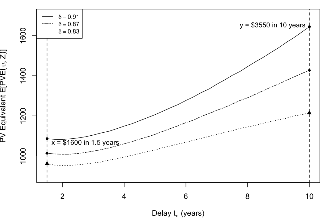
Figure 12: Simulated average present value equivalents $E[PVE(\upsilon,Z)]$ for delayed payments $\nu=(m_{\upsilon},t_{\upsilon})$ with present value equal to that of $x=(1600,1.5)$ for $\delta=0.91$ as a function of $t_{\upsilon}$. In these simulations, $Z$ is adapted to $\upsilon$, and we set $|Z|=15$. $\tau_{xy}$ has a CPF-complexity representation parameterized by $H(r)=(\Phi^{-1}(G(r)))^{2}$, for $G$ given by (1) with $\kappa=0,\gamma=0.75$. Priors are distributed $Q\sim U[0,1]$.

B.6 Apparent Biases in Intertemporal Valuations

We work in the same setting as in Appendix B.5. Consider a standard paradigm used to estimate the discount function: the DM values delayed payments $\upsilon=(\overline{m},t_{\upsilon})$ terms of money today. Figure 13 plots the normalized valuations $E[PVE(\nu,Z)]/\overline{m}$ as a function of the delay $t_{\upsilon}$, where $\upsilon$ is valued against a price list $Z=(z^{1},...,z^{n})$ of immediate payments adapted to $\upsilon$. As the figure shows, the DM’s valuations display apparent hyperbolicity: she undervalues payments close to the present and overvalues payments with longer delays.

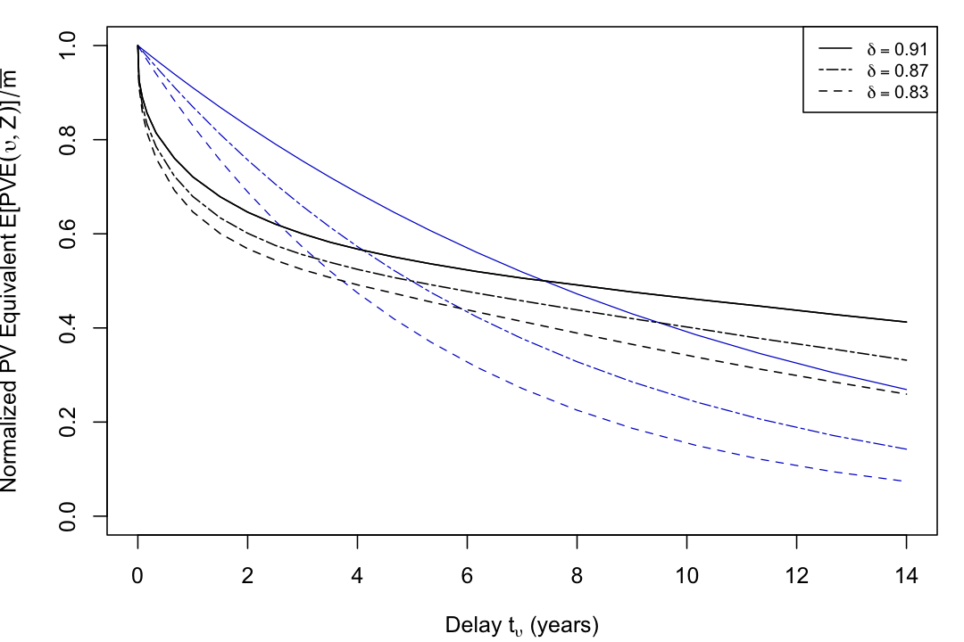
Figure 13: Simulated average present value equivalents $E[PVE(\upsilon,Z)]$ (in black) for delayed payments $\nu=(\overline{m},t_{\upsilon})$ as a function of $t_{\upsilon}$. Blue curves plot distortion-free present values given the true discount rate $\delta$. In these simulations, $Z$ is adapted to $\upsilon$, and we set $|Z|=15$. $\tau_{xy}$ has a CPF-complexity representation parameterized by $H(r)=(\Phi^{-1}(G(r)))^{2}$, for $G$ given by (1) with $\kappa=0,\gamma=0.75$. Priors are distributed $Q\sim U[0,1]$.

Now consider an alternative paradigm that should reveal the same preferences as the paradigm above in the absence of complexity-driven distortions. The DM asses the time equivalents of an immediate payment: the delay $t$ that makes the delayed payment $(\overline{m},t)$ indifferent to the immediate payment $c=(m_{c},0)$.

Formally, the DM values each delayed payment $c=(m_{c},0)$ against a time list $Z=(z^{1},...z^{n})$, where each $z^{k}=(\overline{m},t_{k})$, for $t_{1}<t_{2}<...,t_{n}$. We restrict attention to time lists with $t_{1}=0$. Let

$$TE(c,Z) =\begin{cases}1/2[t_{R(c,Z)-1}+t_{R(c,Z)}]&R(c,Z)<n+1\\ t_{n}+1/2(t_{n}-t_{n-1})&R(x,Z)=n+1\end{cases}$$

denote the distribution over the DM’s time equivalents obtained from assigning each switching point to a valuation at the midpoint of the adjacent delays.

Figure 14 plots the predicted relationship between the immediate payment amount $m_{c}/\overline{m}$ (y-axis) and the associated time equivalents $E[TE(c,Z)]$ (x-axis). Here, the model predicts an apparent reversal of hyperbolic discounting: the difficulty of comparing immediate payments to the numeraire good causes time equivalents to compressed towards the middle of the price list, generating overvaluation of payments close to the present and undervaluation of payments with longer delays.

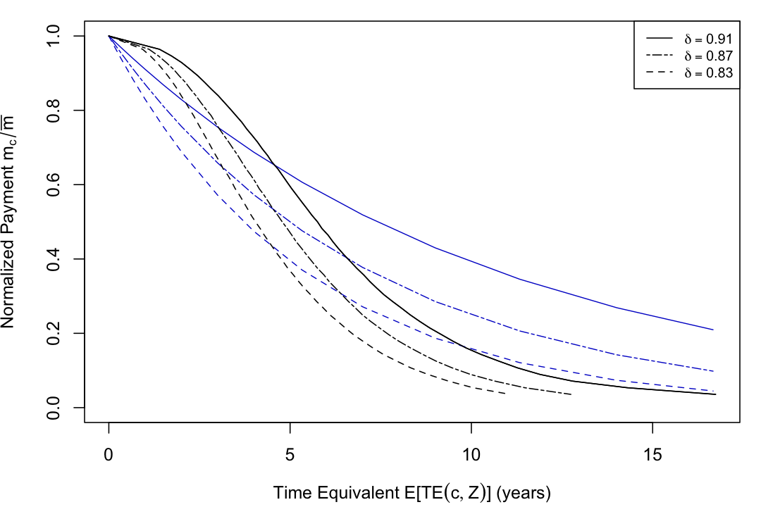
Figure 14: Relationship between simulated average time equivalents $E[TE(c,Z)]$ (in black) for the immediate payment $c=(m_{c},0)$ and the normalized payment amount $m_{c}/\overline{m}$. Blue curves plot distortion-free time equivalents given the true discount rate $\delta$. In these simulations, $Z=(z^{1},...,z^{n})$, where where $z^{k}=(\overline{m},t_{k})$, for $(t_{1},...,t_{n})=(0,2,4,8,12,18,24,36,48,64,84,108,136,168,200)$ months. $\tau_{xy}$ has a CPF-complexity representation parameterized by $H(r)=(\Phi^{-1}(G(r)))^{2}$, for $G$ given by (1) with $\kappa=0,\gamma=0.75$. Priors are distributed $Q\sim U[0,1]$.

Appendix C Appendix: Proofs

C.1 Characterization Results

Begin with some basic definitions and observations. Let $X$ be a space of options, and let $\mathcal{D}=\{(x,y)\in X\times X:x\neq y\}$. Say $\rho:\mathcal{D}\to[0,1]$ is a binary choice rule on $X$ if $\rho(x,y)=1-\rho(y,x)$.

Call a (complete) binary relation $\succeq$ on $X$ the stochastic order induced by a binary choice rule $\rho$ if for all $x\neq y$, $x\succeq y$ if $\rho(x,y)\geq 1/2$, and for all $x\in X$, $x\succeq x$. Say that a binary choice rule $\rho$ satisfies moderate transitivity if for $\rho(x,y),\rho(y,z)\geq 1/2$, then $\rho(x,z)>\min\{\rho(x,y),\rho(y,z)\}$ or $\rho(x,z)=\rho(x,y)=\rho(y,z)$. Say that a binary choice rule $\rho$ satisfies weak transitivity if for $\rho(x,y),\rho(y,z)\geq 1/2$, $\rho(x,y)\geq 1/2$. Consider a partial order $\geq_{X}$ on $X$. Say that a binary choice rule $\rho$ satisfies monotonicity with respect to $\geq_{X}$ if $x^{\prime}\geq_{X}x$ implies $\rho(x^{\prime},y)\geq\rho(x,y)$, where the inequality is strict whenever $x\not\geq_{X}x^{\prime}$, $x\not\geq_{X}y$ and $y\not\geq_{X}x$. Say that $\rho$ satisfies dominance with respect $\geq_{X}$ if whenever $x\geq_{X}y$, we have $\rho(x,y)\geq\rho(w,z)$ for all $w,z\in X$, where the inequality is strict if $w\not\geq_{X}z$.

Lemma 1.

If $\rho$ defined on $X$ satisfies moderate transitivity and dominance with respect to a partial order $\geq_{X}$, then it satisfies monotonicity with respect to $\geq_{X}$.

Proof.

Take any options $x,y$, and suppose $x^{\prime}\geq_{X}x$. If $x\geq_{X}x^{\prime}$, then $x^{\prime}=x$ since $\geq_{X}$ is a partial order and is therefore antisymmetric, and we are done. Now consider the case where $x\not\geq_{X}x^{\prime}$. Note that if $x\geq_{X}y$, since $\geq_{X}$ is transitive we also have $x^{\prime}\geq_{X}y$, and so Dominance implies that $\rho(x^{\prime},y)\geq\rho(x,y)$ and we are done.

Now consider the case where $x\not\geq_{X}y$. Let $\succeq$ denote the stochastic order induced by $\rho$; since $\rho$ satisfies MST, $\succeq$ is complete and transitive. By dominance, we have $\rho(x^{\prime},x)>\rho(x,x^{\prime})\implies\rho(x^{\prime},x)>1/2$ and so $x^{\prime}\succ x$. There are three cases to consider:

Case 1: $x^{\prime}\succeq x\succeq y$. By moderate transitivity, $\rho(x^{\prime},y)>\min\{\rho(x^{\prime},x),\rho(x,y)\}$ or $\rho(x^{\prime},y)=\rho(x^{\prime},x)=\rho(x,y)$. But since $\rho(x^{\prime},x)>\rho(x,y)$ by dominance, it must be the case that $\rho(x^{\prime},y)>\rho(x,y)$.

Case 2: $x^{\prime}\succeq y\succeq x$. By definition of $\succeq$, $\rho(x^{\prime},y)\geq 1/2\geq\rho(x,y)$. Also, since $x^{\prime}\succ x$, we must have one of $x^{\prime}\succ y$ or $y\succ x$, and so by definition of $\succeq$ we must have one of $\rho(x^{\prime},y)>1/2$ or $1/2>\rho(x,y)$, which implies $\rho(x^{\prime},y)>\rho(x,y)$.

Case 3: $y\succeq x^{\prime}\succeq x$. Toward a contradiction, suppose that $\rho(y,x^{\prime})>\rho(y,x)$. By moderate transitivity, we have $\rho(y,x)>\min\{\rho(y,x^{\prime}),\rho(x^{\prime},x)\}$ which implies $\rho(y,x)>\rho(x^{\prime},x)$, which contradicts dominance and so $\rho(y,x^{\prime})\leq\rho(y,x)\implies\rho(x^{\prime},y)\geq\rho(x,y)$.

All that remains is to show that $\rho(x^{\prime},y)>\rho(x,y)$ when $x\not\geq_{X}y$ and $y\not\geq_{X}x$. We have already shown that the inequality is strict in Cases 1 and 2; all that remains is to show that the inequality is strict in Case 3. Suppose $y\succeq x^{\prime}\succeq x$. Toward a contradiction, suppose that $\rho(y,x^{\prime})\geq\rho(y,x)$. Moderate transitivity then implies that either (i) $\rho(y,x)>\min\{\rho(y,x^{\prime}),\rho(x^{\prime},x)\}$ or (ii) $\rho(y,x)=\rho(y,x^{\prime})=\rho(x^{\prime},x)$. As we saw above, it cannot be the case that (i) holds. If (ii) holds, then dominance implies that $y\geq x$, a contradiction. ∎

For the following result, we consider the case where $X$ is a convex set. Say $\rho$ is linear if $\rho(x,y)=\rho(\lambda x+(1-\lambda)z,\lambda y+(1-\lambda)z)$ for all $x,y,z\in X$, $\lambda\in(0,1)$. Say $\rho$ is superadditive if for any $x,y,x^{\prime},y^{\prime}$ with $\rho(x,y),\rho(x^{\prime},y^{\prime})\geq 1/2$, for any $\lambda\in[0,1]$ we have $\rho(\lambda x+(1-\lambda)x^{\prime},\lambda y+(1-\lambda)y^{\prime})\geq\min\{\rho(x,y),\rho(x^{\prime},y^{\prime})\}$.

Lemma 2.

Let $X$ be a vector space. If $\rho$ defined on $X$ satisfies moderate transitivity and linearity, then $\rho$ is superadditive.

Proof.

Since $X$ is a vector space and so contains additive inverses, linearity implies $\rho(x,y)=\rho(Cx,Cy)$ and $\rho(x,y)=\rho(x-z,y-z)$ for any for any $C>0,x,y,z\in X$. Now consider $x,y,x^{\prime},y^{\prime}$ with $\rho(x,y),\rho(x^{\prime},y^{\prime})\geq 1/2$, and $\lambda\in[0,1]$. The above implies that

$$\rho(\lambda(x-y),0) =\rho(x,y)\geq 1/2$$

$$\rho(0,-(1-\lambda)(x^{\prime}-y^{\prime})) =\rho(x^{\prime},y^{\prime})\geq 1/2$$

$$\rho(\lambda x+(1-\lambda)x^{\prime},\lambda y+(1-\lambda)y^{\prime}) =\rho(\lambda(x-y),-(1-\lambda)(x^{\prime}-y^{\prime}))$$

This, in conjunction with moderate transitivity, implies that

$$\rho(\lambda x+(1-\lambda)x^{\prime},\lambda y+(1-\lambda)y^{\prime}) =\rho(\lambda(x-y),-(1-\lambda)(x^{\prime}-y^{\prime}))$$

$$\geq\min\{\rho(\lambda(x-y),0),\rho(0,-(1-\lambda)(x^{\prime}-y^{\prime}))\}$$

$$=\min\{\rho(x,y),\rho(x^{\prime},y^{\prime})\}$$

∎

Proof of Theorem 1.

Necessity of the axioms is immediate from the definition. We now show sufficiency.

Assume that M1–M5 holds. Let $\succeq$ denote the stochastic order on $\mathbb{R}^{n}$ induced by $\rho$. By weak transitivity, $\succeq$ is transitive. Since $\rho$ satisfies Continuity and Linearity, $\succeq$ satisfies axioms D1–D3 of Theorem 9.1 of Gilboa, (2009). Invoking an intermediate step in the proof of this theorem, we conclude that there exists weights $\beta\in\mathbb{R}^{n}$ such that $U(x)=\sum_{k}\beta_{k}x_{k}$ represents $\succeq$. Since all attributes are non-null, we have that $\beta_{k}\neq 0$ for all $k$. For the remainder of the proof, we henceforth identify each option $x$ with its weighted attribute values, so that $U(x)=\sum_{k}x_{k}$. Since $\rho$ satisfies Dominance and MST, Lemma 1 implies that $\rho$ satisfies monotonicity with respect to the component-wise dominance relation on $\mathbb{R}^{n}$.

For $z\in\mathbb{R}^{n}$, Let $d^{+}(z)=\sum_{k:z_{k}\geq 0}z_{k}$ and $d^{-}(x)=\sum_{k:z_{k}<0}|z_{k}|$ denote the summed advantages and disadvantages in the comparison between $z$ and $0$. Say that $z$ has no dominance relationship if $d^{+}(z),d^{-}(z)>0$.

Claim 1. For any $z\in\mathbb{R}^{n}$ satisfying $\sum_{k}z_{k}\geq 0$, $\rho(z,0)=\rho(d^{+}(z)e_{1}-d^{-}(z)e_{2},0)$.

Proof.

For $i,j\in\{1,...,n\}$, $i\neq j$, define $z^{ij}\in\mathbb{R}^{n}$ satisfying

$$z^{ij}_{k}=\begin{cases}d^{+}(z)&k=i\\ -d^{-}(z)&k=j\\ 0&\text{otherwise}\end{cases}$$

Note that because we have normalized utility weights 1, for all $i\neq j$, $l\neq m$, we have $U(z^{ij})=d^{+}(z)-d^{-}(z)=U(z^{lm})$, and so $z^{ij}\sim z^{lm}$. We will first show that $\rho(z^{ij},0)=\rho(z^{lm},0)$ for all $i\neq j,l\neq m$. It is sufficient to show that for all $i,j$ $\rho(z^{ij},0)=\rho(z^{12},0)$. There are two cases to consider:

Case 1: $j>i$. Since $z^{1j}\sim z^{ij}$, and since $z^{1j}_{i}=0$, $z^{1j}_{k}=z^{ij}_{k}$ for all $k\neq i,1$, Simplification implies that $\rho(z^{1j},0)\geq\rho(z^{ij},0)$. Also, since $z^{ij}_{1}=0$, and $z^{ij}_{k}=z^{1j}_{k}$ for all $k\neq 1,i$, Simplification implies $\rho(z^{1j},0)\leq\rho(z^{ij},0)$, and so $\rho(z^{1j},0)=\rho(z^{ij},0)$. A analogous argument yields $\rho(z^{12},0)=\rho(z^{1j},0)$, and so $\rho(z^{ij},0)=\rho(z^{12},0)$.

Case 2: $j<i$. By analogous arguments as above, we have $\rho(z^{ij},0)=\rho(z^{nj},0)$, $\rho(z^{nj},0)=\rho(z^{n2},0)$ and $\rho(z^{n2},0)=\rho(z^{12},0)$, and so $\rho(z^{ij},0)=\rho(z^{12},0)$ as desired.

Let $K^{+}=\{i\in\{1,2,...,n\}:z_{i}\geq 0\}$ and $K^{-}=\{i\in\{1,2,...,n\}:z_{i}<0\}$. Defining $\lambda_{i}=\frac{z_{i}}{\sum_{k\in K^{+}}{z_{k}}}$ for $i\in K^{+}$, and $\gamma_{j}=\frac{z_{j}}{\sum_{k\in K^{-}}z_{k}}$ for $j\in K^{-}$, note that $z=\sum_{i\in K^{+}}\sum_{j\in K^{-}}\lambda_{i}\gamma_{j}z^{ij}$, and so $z$ can be expressed as a mixture of $z^{ij}$’s. Since $\rho$ satisfies superadditivity by Lemma 2, by inductive application of superadditivity, we have $\rho(z,0)\geq\rho(z^{ij},0)$ for all $i\neq j$, which in turn implies $\rho(z,0)\geq\rho(z^{12},0)$.

Note that by repeated application of Simplification, we have $\rho(z,0)\leq\rho(z^{ij},0)$, for some $i$ where $z_{i}\geq 0$, and some $j$ where $z_{j}\leq 0$. Since $\rho(z^{ij},0)=\rho(z^{12},0)$, we have $\rho(z,0)\leq\rho(z^{12},0)$, and so $\rho(z,0)=\rho(z^{12},0)$ as desired. ∎

Claim 2. For $z$ with $\sum_{k}z_{k}\geq 0$, $\rho(z,0)=\tilde{G}\left(\frac{d^{+}(z)-d^{-}(z)}{d^{+}(z)+d^{-}(z)}\right)$ for some strictly increasing, continuous $\tilde{G}:[0,1]\to\mathbb{R}$.

Proof.

Fix any $z$ with $\sum_{k}z_{k}\geq 0$, and consider the case where $z$ has no dominance relationship, that is $d^{+}(z)>0$, $d^{-}(z)>0$. By Claim 1, we have $\rho(z,0)=\rho(d^{+}(z)e_{1}-d^{-}e_{2},0)$. Define $F:[1,\infty)\to[1/2,1)$ by $F(t)=\rho(te_{1}-e_{2},0)$; by monotonicity, of $\rho$, $F$ is strictly increasing. By Linearity, we have $\rho(d^{+}(z)e_{1}-d^{-}e_{2},0)=\rho((d^{+}(z)/d^{-}(z))e_{1}-e_{2},0)=F(d^{+}(z)/d^{-}(z))$.

Let $\varphi(z)=\frac{z-1}{z+1}$; and define $\tilde{G}:[0,1)\to\mathbb{R}$ where $\tilde{G}(z)=F(\varphi^{-1}(z))$; since $\varphi$ and $F$ are strictly increasing, $\tilde{G}$ is strictly increasing. By construction, we have $F(z)=\tilde{G}\left(\frac{z-1}{z+1}\right)$, and so $\rho(z,0)=\rho(d^{+}(z)e_{1}-d^{-}e_{2},0)=\tilde{G}\left(\frac{d^{+}(z)-d^{-}(z)}{d^{+}(z)+d^{-}(z)}\right)$. Since $\rho$ is continuous, $\tilde{G}$ is continuous on its domain $[0,1)$, and in particular is uniformly continuous since it is increasing and bounded. Take the continuous extension of $\tilde{G}$ to $[0,1]$.

Now consider the case where $z$ has a dominance relationship; that is $d^{+}(z)>0$, $d^{-}(z)=0$. By Dominance, $\rho(z,0)=\rho(d^{+}(z)e_{1}-d^{-}e_{2},0)$ takes on some constant value $q$ such that $q>\rho(z^{\prime},0)$ for all $z^{\prime}$ without a dominance relationship, which implies that $q>\tilde{G}(t)$ for all $t\in[0,1)$. Since $\rho$ is continuous, it must be the case that $q=\tilde{G}(1)$. ∎

Now, let $G:[-1,1]\to\mathbb{R}$ be the symmetric extension of $\tilde{G}$ satisfying

$$G(z)=\begin{cases}\tilde{G}(z)&z\geq 0\\ 1-\tilde{G}(-z)&z<0\end{cases}$$

Claim 3. For any $z$, $\rho(z,0)=G\left(\frac{d^{+}(z)-d^{-}(z)}{d^{+}(z)+d^{-}(z)}\right)$.

Proof.

Claim 1 implies that $\rho(z,0)=G\left(\frac{d^{+}(z)-d^{-}(z)}{d^{+}(z)+d^{-}(z)}\right)$ whenever $\sum_{k}z_{k}\geq 0$. Now consider the case where $\sum_{k}z_{k}<0$. Note that

$$\rho(z,0) =1-\rho(-z,0)$$

$$=1-\tilde{G}\left(\frac{d^{-}(z)-d^{+}(z)}{d^{+}(z)+d^{-}(z)}\right)$$

$$=G\left(\frac{d^{+}(z)-d^{-}(z)}{d^{+}(z)+d^{-}(z)}\right)$$

as desired, where the first equality uses symmetry and Linearity of $\rho$ and the second equality uses Claim 2. ∎

Take any $x,y$, and let $z=x-y$. Due to linearity, we have

$$\rho(x,y) =\rho(z,0)$$

$$=G\left(\frac{d^{+}(z)-d^{-}(z)}{d^{+}(z)+d^{-}(z)}\right)$$

$$=G\left(\frac{\sum_{k}z_{k}}{\sum_{k}|z_{k}|}\right)$$

$$=G\left(\frac{U(x)-U(y)}{d_{L1}(x,y)}\right)$$

as desired.

Finally, to show uniqueness, suppose $(G,\beta)$ and $(G^{\prime},\beta^{\prime})$ both represent $\rho$. Define the stochastic preference relation $\succeq$ as before. Since $G$ and $G^{\prime}$ are both strictly increasing and symmetric around 0, $U(x)=\sum_{k}\beta_{k}x_{k}$ and $U^{\prime}(x)=\sum_{k}\beta^{\prime}_{k}x_{k}$ both represent $\succeq$, and so there exists $C>0$ such that $\beta^{\prime}_{k}=C\beta_{k}$. This in turn implies that for all $z\in\mathbb{R}^{n}$, we have

$$G\left(\frac{\sum_{k}\beta_{k}z_{k}}{\sum_{k}|\beta_{k}z_{k}|}\right) =G^{\prime}\left(\frac{\sum_{k}\beta^{\prime}_{k}z_{k}}{\sum_{k}|\beta^{\prime}_{k}z_{k}|}\right)$$

$$=G^{\prime}\left(\frac{\sum_{k}\beta_{k}z_{k}}{\sum_{k}|\beta_{k}z_{k}|}\right)$$

Let $z=\alpha/\beta_{1}e_{1}+\gamma/\beta_{2}e_{2}$. Note that for any $r\in[-1,1]$, there exists $\alpha,\gamma$ such that $\frac{\sum_{k}\beta_{k}z_{k}}{\sum_{k}|\beta_{k}z_{k}|}=\frac{\alpha-\gamma}{|\alpha+\gamma|}=r$, and so $G^{\prime}(r)=G(r)$ for all $r\in[-1,1]$.

$\square$

Proof of Theorem 2.

The proof of necessity is routine. Theorem 1 covers sufficiency for the $n\geq 3$ case. We now show sufficiency in the case where $n=2$; assume that M1–M6 hold. Note that Claim 1 in the proof of Theorem 1 continues to hold in this case; that is, that for any $z\in\mathbb{R}^{n}$ satisfying $\sum_{k}z_{k}\geq 0$, $\rho(z,0)=\rho(d^{+}(z)e_{1}-d^{-}(z)e_{2},0)$. To see this, note that if $z_{1}\geq 0$, $z_{2}\geq 0$, the desired equality follows from Dominance; if not then either i) $z_{1}>0$, $z_{2}<0$ or ii) $z_{1}<0$ and $z_{2}>0$. In case i), the equality is immediate since $z=d^{+}e_{1}+d^{-}e_{2}$, which in conjunction with Exchangeability, implies the desired equality for case ii). Following the steps in Claims 2 and 3 in the proof of Theorem 1 completes the proof of sufficiency. Note that the argument for uniqueness in Theorem 1 holds for $n=2$, and so uniqueness holds as well.

$\square$

Proof of Theorem 3.

The proof of necessity of M1, M4–M5, and M7 are routine. To see that M3 (Moderate Transitivity) is necessary, consider $x,y,z$ with $\rho(x,y)\geq 1/2$ and $\rho(y,z)\geq 1/2$. If $d_{L1}(x,y),d_{L1}(y,z)$, $d_{L1}(x,z)>0$, then the restriction of $\rho$ to $\{x,y,z\}$ belongs to the moderate utility class studied in He and Natenzon, (2023) and so by Theorem 1 of this paper we can conclude that this restriction satisfies Moderate Transitivity. There are four additional cases to consider. Case 1: suppose $d_{L1}(x,y)=0$. We then have $\rho(x,z)=\rho(y,z)$ and $\rho(x,y)=1/2$, so either $\rho(x,z)>\min\{\rho(x,y),\rho(y,z)\}$ or $\rho(x,z)=\rho(y,z)=\rho(x,z)$. Case 2: $d_{L1}(y,z)=0$. We then have $\rho(x,z)=\rho(x,y)$ and $\rho(y,z)=1/2$, and so again either $\rho(x,z)>\min\{\rho(x,y),\rho(y,z)\}$ or $\rho(x,z)=\rho(y,z)=\rho(x,z)$. Case 3: $d_{L1}(x,z)=0$. Here we have $\rho(x,z)=1/2$, and $\rho(x,y)=\rho(z,y)\geq 1/2$ and $\rho(y,z)\geq 1/2$, which implies $\rho(y,z)=\rho(x,y)=1/2$; we therefore have $\rho(x,y)=\rho(y,z)=\rho(x,z)$. Finally, consider $d_{L1}(x,y)=d_{L1}(x,z)=d_{L1}(y,z)=0$; here we have $\rho(x,y)=\rho(y,z)=\rho(x,z)$, and so Moderate Transitivity holds in all cases.

To see that M8 (Tradeoff Congruence) is necessary, take $(x,y),(y,z)\in\mathcal{D}$ congruent such that $\rho(x,y),\rho(y,z)\geq 1/2$. Note that if $d_{L1}(x,z)=0$, then $\rho(x,y)=1/2$ and since $\rho$ satisfies Moderate Transitivity we have $\rho(x,y)=\rho(y,z)=1/2$ and we are done. Now consider the case where $\rho(x,z)\neq 0$. Note that

$$\rho(x,z) =G\left(\frac{\sum_{k}(u_{k}(x_{k})-u_{k}(z_{k}))}{\sum_{k}|u_{k}(x_{k})-u_{k}(z_{k})|}\right)$$

$$=G\left(\frac{\sum_{k}(u_{k}(x_{k})-u_{k}(y_{k})+u_{k}(y_{k})-u_{k}(z_{k}))}{\sum_{k}|u_{k}(x_{k})-u_{k}(y_{k})+u_{k}(y_{k})-u_{k}(z_{k})|}\right)$$

$$=G\left(\frac{U(x)-U(y)+U(y)-U(z)}{d_{L1}(x,y)+d_{L1}(y,z)}\right)$$

Where the final equality holds because congruence implies that $u_{k}(x_{k})-u_{k}(y_{k})$ and $u_{k}(y_{k})-u_{k}(z_{k})$ must either be both positive or negative. This implies that if either $d_{L1}(x,y)=0$ or $d_{L1}(y,z)=0$, we are done. Now consider the case where $d_{L1}(x,y),d_{L1}(y,z)>0$, and suppose $\rho(y,z)\leq\rho(x,y)$; this implies $\frac{U(y)-U(z)}{d_{L1}(y,z)}\leq\frac{U(x)-U(y)}{d_{L1}(x,y)}$. The above implies

$$\rho(x,z) =G\left(\frac{\frac{U(x)-U(y)}{d_{L1}(y,z)}+\frac{U(y)-U(z)}{d_{L1}(y,z)}}{\frac{d_{L1}(x,y)}{d_{L1}(y,z)}+1}\right)$$

$$\leq G\left(\frac{\frac{U(x)-U(y)}{d_{L1}(y,z)}+\frac{U(x)-U(y)}{d_{L1}(x,y)}}{\frac{d_{L1}(x,y)}{d_{L1}(y,z)}+1}\right)$$

$$=\rho(x,y)$$

and so $\rho(x,z)\leq\max\{\rho(x,y),\rho(y,z)\}$ when $\rho(y,z)\leq\rho(x,y)$. The argument for the case where $\rho(y,z)\geq\rho(x,y)$ is analogous.

Now we show sufficency. Let $\succeq$ be the stochastic preference relation induced by $\rho$. $\succeq$ satisfies coordinate independence and inherits continuity from $\rho$, and since we have at least 3 non-null attributes, we invoke Debreu, (1983) to conclude that $\succeq$ has an additively separable representation: there exists $u_{i}:X_{i}\to\mathbb{R}$, continuous, such that

$$x\succeq y\iff\sum_{k}u_{k}(x_{k})\geq\sum_{k}u_{k}(y_{k})$$

Since all attributes are non-null and the $X_{k}$ are connected, each $u_{k}(X_{k})$ is a non-trivial interval of $\mathbb{R}$. Since the representation is unique up to cardinal transformations, we can without loss assume that for each $k\in I$, $u_{k}(X_{k})$ contains $0$, and furthermore, since $u_{k}(X_{k})$ is a non-trivial interval, that $u_{k}(X_{k})$ contains a non-trivial open interval around $0$. For all $k\in I$, let $\overline{u}_{k}=\sup u_{k}(X_{k})$ and $\underline{u}_{k}=\inf u_{k}(X_{k})$, taken with respect to the extended real line, and let $\Delta_{k}=\overline{u}_{k}-\underline{u}_{k}$. For all $x\in X$, define $\tilde{x}=(u_{1}(x_{1}),...,u_{k}(x_{k}))\in\mathbb{R}^{n}$. Begin by noting the following result.

Lemma 3.

For $x,y\in X$ with $\tilde{x}=\tilde{y}$: $\rho(x,z)=\rho(y,z)$ for all $z\in X$.

Proof.

Fix such an $x,y$, and take any $z\in X$. Note that $x\sim y$ by hypothesis. First consider the case where $x\sim y\succeq z$. Since $(x,y)$ and $(y,z)$ are congruent, and likewise $(y,x)$ and $(x,z)$ are congruent, Tradeoff Congruence implies

$$\rho(x,z)\leq\max\{\rho(y,z),\rho(x,y)\}=\rho(y,z)$$

$$\rho(y,z)\leq\max\{\rho(x,z),\rho(y,x)\}=\rho(x,z)$$

and so $\rho(y,z)=\rho(x,z)$. Analogously, consider the case where $z\succeq x\sim y$. Since $(z,x)$ and $(x,y)$ are congruent and likewise $(z,y)$ and $(y,x)$ are congruent, we have

$$\rho(z,x)\leq\max\{\rho(z,y),\rho(y,x)\}=\rho(z,y)$$

$$\rho(z,y)\leq\max\{\rho(z,x),\rho(x,y)\}=\rho(z,x)$$

and so $\rho(z,x)=\rho(z,y)\implies\rho(x,z)=\rho(y,z)$. ∎

Let $\tilde{X}=\{\tilde{x}\in\mathbb{R}^{n}:x\in X\}$. Let $\tilde{\mathcal{D}}=\{(a,b)\in\tilde{X}:a\neq b\}$ and define $\phi:\tilde{\mathcal{D}}\to\mathcal{D}$ satisfying $\phi(a,b)\in\{(x,y)\in\mathcal{D}:\tilde{x}=a,\tilde{y}=b\}$, and define $\tilde{\rho}:\tilde{\mathcal{D}}\to[0,1]$ by $\tilde{\rho}(a,b)=\rho(\phi(a,b))$. Lemma 3 implies that $\tilde{\rho}$ is a binary choice rule on $\tilde{\mathcal{D}}$ and does not depend on the selection made by $\phi$: in particular, we have $\tilde{\rho}(\tilde{x},\tilde{y})=\rho(x,y)$ for all $(x,y)\in\mathcal{D}$. This in turn implies that $\tilde{\rho}$ inherits our axioms M1,M3–M5, M7–M8. Note that if there exists a strictly increasing, continuous function $G$ such that

$$\tilde{\rho(a,b)}=G\left(\frac{\sum_{k}(a_{k}-b_{k})}{\sum_{k}|a_{k}-b_{k}|}\right)$$

for all $(a,b)\in\mathcal{D}$, we are done, as this implies that for any $(x,y)\in\mathcal{D}$ such that $\tilde{x}\neq\tilde{y}\iff\sum_{k}|u_{k}(x_{k})-u_{k}(y_{k})|>0$,

$$\rho(x,y)=\tilde{\rho}(\tilde{x},\tilde{y})=G\left(\frac{\sum_{k}(u_{k}(x_{k})-u_{k}(y_{k}))}{\sum_{k}|u_{k}(x_{k})-u_{k}(y_{k})|}\right)$$

and furthermore for $(x,y)\in\mathcal{D}$ such that $\tilde{x}=\tilde{y}$, we have $x\sim y\implies\rho(x,y)=1/2$, and so $\rho$ has an additively separable $L_{1}$-complexity representation.

In what follows, we will work with $\tilde{\rho}$ defined on $\tilde{X}$ and suppress the $\sim$ in our notation. Say that $\rho$ defined on this domain is

• Translation invariant if for all $x,x^{\prime},y,y^{\prime}\in X,z\in\mathbb{R}^{n}$ such that $x^{\prime}=x+z$, $y^{\prime}=y+z$, $\rho(x^{\prime},y^{\prime})=\rho(x,y)$.

• Scale invariant if for all $x,x^{\prime},y,y^{\prime}\in X$ such that $x^{\prime}=cx,y^{\prime}=cy$ for $c>0$, $\rho(x^{\prime},y^{\prime})=\rho(x,y)$.

• Translation invariant* if for all $x,x^{\prime},y,y^{\prime}\in X,z\in\mathbb{R}^{n}$ such that $x^{\prime}=x+z$, $y^{\prime}=y+z$, and additionally $x_{k}=y_{k}$ for some $k\in I$, $\rho(x^{\prime},y^{\prime})=\rho(x,y)$.

• Scale invariant* if for all $x,x^{\prime},y,y^{\prime}\in X$ such that $x^{\prime}=cx,y^{\prime}=cy$ for $c>0$, and additionally $x_{k}=y_{k}$ for some $k\in I$, $\rho(x^{\prime},y^{\prime})=\rho(x,y)$.

• Translation invariant^† if for all $x,x^{\prime},y,y^{\prime}\in X,z\in\mathbb{R}^{n}$ such that $x^{\prime}=x+z$, $y^{\prime}=y+z$, and additionally $x_{k}=y_{k}$ for some $k\in I$ such that $|x_{i}-y_{i}|<\Delta_{k}$ for all $i\in I$, $\rho(x^{\prime},y^{\prime})=\rho(x,y)$.

• Scale invariant^† if for all $x,x^{\prime},y,y^{\prime}\in X$ such that $x^{\prime}=\lambda x,y^{\prime}=\lambda y$ for $\lambda\in(0,1)$, and additionally $x_{k}=y_{k}$ for some $k\in I$ such that $|x_{i}-y_{i}|<\Delta_{k}$ for all $i\in I$, $\rho(x^{\prime},y^{\prime})=\rho(x,y)$.

First, note that Separability and Simplification imply translation invariance^†.

Lemma 4.

Suppose $\rho$ satisfies Separability and Simplification. Then $\rho$ satisfies translation invariance^†.

Proof.

Begin by noting that for $x^{\prime},y^{\prime},x,y\in X$, $z\in\mathbb{R}^{n}$ with $x^{\prime}=x+z$, $y^{\prime}=y+z$, and $x_{k}=y_{k}$ for some $k\in I$ such that $|x_{i}-y_{i}|<\Delta_{k}$ for all $i\in I$: for any $E\subseteq I$, $x+\sum_{j\in E}z_{\{j\}}$ and $y+\sum_{j\in E}z_{\{j\}}$ will be in our domain, with $\left(x+\sum_{j\in E}z_{\{j\}}\right)_{k}=\left(y+\sum_{j\in E}z_{\{j\}}\right)_{k}$ and with $\left|\left(x+\sum_{j\in E}z_{\{j\}}\right)_{i}-\left(y+\sum_{j\in E}z_{\{j\}}\right)_{i}\right|<\Delta_{k}$ for all $i$. Since we can translate $x$ and $y$ by each component $z_{\{j\}}$ attribute-by-attribute, it suffices to show that for any $x,y\in X$ with $x_{k}=y_{k}$ where $|x_{i}-y_{i}|<\Delta_{k}$ for all $i\in I$, $z\in\mathbb{R}^{n}$, $j\in I$ such that $x+z_{\{j\}}$ and $y+z_{\{j\}}$ belong to our domain, $\rho(x+z_{\{j\}},y+z_{\{j\}})=\rho(x,y)$. Fix such an $x,y\in X$, $z\in\mathbb{R}^{n}$, $k,j\in I$.

Note that if $j=k$, Separability gives us the desired result. Now suppose $j\neq k$. Suppose that $x_{j}\geq y_{j}$ (the argument for $x_{j}<y_{j}$ is analogous). For any $i\in I$, $a\in(\underline{u}_{i},\overline{u}_{i})$, $w\in X$, let $a_{\{i\}}w\in X$ denote the option equal to $a$ for attribute $k=i$ and equal to $w_{k}$ for all other attributes. Since by hypothesis $|x_{i}-y_{i}|<\Delta_{k}$ for all $i$, there exists some $b\in(\underline{u}_{k},\overline{u}_{k})$ such that $|x_{i}-y_{i}|<\overline{u}_{k}-b$ for all $i$. By Separability, we have $\rho(b_{\{k\}}x,b_{\{k\}}y)=\rho(x,y)$. Now consider $x^{\prime}\in\mathbb{R}^{n}$ satisfying

$$x^{\prime}_{i}=\begin{cases}y_{j}&i=j\\ b+(x_{j}-y_{j})&i=k\\ x_{i}&\text{otherwise}\end{cases}$$

By construction, $b+(x_{j}-y_{j})<\overline{u}_{k}$, and so $x^{\prime}\in X$. Applying simplification twice, we have $\rho(x^{\prime},b_{\{k\}}y)=\rho(b_{\{k\}}x,b_{\{k\}}y)$. Since $x^{\prime}_{j}=(b_{\{k\}}y)_{j}$ by construction, Separability in turn implies that $\rho(x^{\prime}+z_{\{j\}},b_{\{k\}}y+z_{\{j\}})=\rho(x^{\prime},b_{\{k\}}y)$. Again applying Simplification twice, we have $\rho(b_{\{k\}}x+z_{\{j\}},b_{\{k\}}y+z_{\{j\}})=\rho(x^{\prime}+z_{\{j\}},b_{\{k\}}y+z_{\{j\}})$. A final application of Separability yields $\rho(x+z_{\{j\}},y+z_{\{j\}})=\rho(b_{\{k\}}x+z_{\{j\}},b_{\{k\}}y+z_{\{j\}})$, and the chain of equalities yields the $\rho(x+z_{\{j\}},y+z_{\{j\}})=\rho(x,y)$ as desired. ∎

The next result says that scale invariance* is implied by translation invariance^† and our other axioms.

Lemma 5.

Suppose $\rho$ satisfies translation invariance^†, Continuity, Moderate Transitivity, and Tradeoff Congruence. Then $\rho$ satisfies scale invariance*.

Proof.

First, show that invariance^† holds for half-mixtures and then extend the result to arbitrary mixtures using continuity. In particular, we want to show that for $x,y\in X$ with $x_{k}=y_{k}$ for some $k$ such that $|x_{i}-y_{i}|<\Delta_{k}$ for all $i$, $\rho(x,y)=\rho(\frac{1}{2}x,\frac{1}{2}y)$. Without loss, suppose that $x\succeq y$. By translation invariance^†, we have $\rho(x,\frac{1}{2}x+\frac{1}{2}y)=\rho(\frac{1}{2}x+\frac{1}{2}y,y)=\rho(\frac{1}{2}x,\frac{1}{2}y)$. Since $(x,\frac{1}{2}x+\frac{1}{2}y)$ and $(\frac{1}{2}x+\frac{1}{2}y,y)$ are congruent and $x\succeq\frac{1}{2}x+\frac{1}{2}y\succeq y$, by Tradeoff Congruence and Moderate Transitivity, we have $\rho(x,y)=\rho(x,\frac{1}{2}x+\frac{1}{2}y)=\rho(\frac{1}{2}x,\frac{1}{2}y)$ as desired.

We now show that for any $x,y\in X$ with $x_{k}=y_{k}$ and $|x_{i}-y_{i}|<\Delta_{k}$ for all $i\in I$, for any $n\in\mathbb{N}$, $\rho(x,y)=\rho(\alpha x,\alpha y)$ for all $\alpha\in\{\frac{1}{2^{n}},\frac{2}{2^{n}},...,\frac{2^{n}}{2^{n}}\}$. Note that if $x\sim y$, then the result holds by definition of $\succeq$ and we are done. Now suppose that $x\not\sim y$, and assume without loss that $x\succ y$. Proceed inductively; given what we have shown above, the statement is true for $n=1$. Now suppose the statement is true for some $n$; we wish to show that for any $m\in\{1,...,2^{n+1}\}$, $\rho(\frac{m}{2^{n+1}}x,\frac{m}{2^{n+1}}y)=\rho(x,y)$. Note that for any $m\leq 2^{n}$ we have $\rho(\frac{m}{2^{n+1}}x,\frac{m}{2^{n+1}}y)=\rho(\frac{m}{2^{n}}x,\frac{m}{2^{n}}y)=\rho(x,y)$ using our result on half-mixtures and by inductive hypothesis.

Now consider $m\in\{2^{n}+1,...,2^{n+1}\}$. Note that by translation invariance^† and by inductive hypothesis, we have $\rho(\frac{m}{2^{n+1}}x,\frac{1}{2}y+\frac{m-2^{n}}{2^{n+1}}x)=\rho(\frac{1}{2}x,\frac{1}{2}y)=\rho(x,y)$. Also, by translation invariance^† and inductive hypothesis, we have $\rho(\frac{1}{2}y+\frac{m-2^{n}}{2^{n+1}}x,\frac{m}{2^{n+1}}y)=\rho(\frac{m-2^{n}}{2^{n+1}}x,\frac{m-2^{n}}{2^{n+1}}y)=\rho(x,y)$. These two equalities and Moderate Transitivity imply that $\rho(\frac{m}{2^{n+1}}x,\frac{m}{2^{n+1}}y)\geq\rho(x,y)$.

Toward a contradiction, suppose $\rho(\frac{m}{2^{n+1}}x,\frac{m}{2^{n+1}}y)>\rho(x,y)$. translation invariance^† then implies $\rho(x,\frac{2^{n+1}-m}{2^{n+1}}x+\frac{m}{2^{n+1}}y)>\rho(x,y)$. By translation invariance^† and the result shown above, we also have $\rho(\frac{2^{n+1}-m}{2^{n+1}}x+\frac{m}{2^{n+1}}y,y)=\rho(\frac{2^{n+1}-m}{2^{n+1}}x,\frac{2^{n+1}-m}{2^{n+1}}y)=\rho(x,y)$. But since Moderate Transitivity implies that $\rho(x,y)>\rho(\frac{2^{n+1-m}}{2^{n+1}}x+\frac{m}{2^{n+1}}y,y)$, we have a contradiction. This proves the statement for $n+1$, and so by induction the statement holds for any $n$. By taking limits and by Continuity of $\rho$, we can then conclude that scale invariance^† holds.

Now we show that scale invariance* holds. Fix any $x,y\in X$ where $x_{k}=y_{k}$ for some $k$. Without loss, assume $x\succeq y$. First, show that $\rho(x,y)=\rho(\lambda x,\lambda y)$ for any $\lambda\in(0,1)$. Note that there exists some $N\in\mathbb{N}$ such that $\frac{1}{N}|x_{i}-y_{i}|<\Delta_{k}$ for all $i$. For $n\in\{0,1,...,N\}$, define $w^{n}\in X$ by $w^{n}=\frac{n}{N}x+\frac{N-n}{N}y$. Now consider the sequence of comparisons $(w^{N},w^{N-1})$, $(w^{N-1},w^{N-2}),...,(w^{1},w^{0})$. Since $w^{n}-w^{n-1}=\frac{1}{N}(x-y)$ for all $n$, we have $w^{n}\succeq w^{n-1}$ for all $n$, and additionally $|w^{n}_{i}-w^{n-1}_{i}|<\Delta_{k}$ for all $i$, and so translation invariance^† implies that for all $n$, $\rho(w^{n},w^{n-1})=\rho(w^{n}-(\frac{N-n}{N}y+\frac{n-1}{N}x),w^{n-1}-(\frac{N-n}{N}y+\frac{n-1}{N}x))=\rho(\frac{1}{N}x,\frac{1}{N}y)$. Sequential applications of Moderate Transitivity and Tradeoff Congruence yield, respectively

$$\rho(x,y)\geq\min\{\rho(w^{N},w^{N-1}),\rho(w^{N-1},w^{N-2}),...,\rho(w^{1},w^{0})\}$$

$$\rho(x,y)\leq\max\{\rho(w^{N},w^{N-1}),\rho(w^{N-1},w^{N-2}),...,\rho(w^{1},w^{0})\}$$

and so we have $\rho(x,y)=\rho(\frac{1}{N}x,\frac{1}{N}y)$. An analogous argument, taking the sequence of comparisons $(\lambda w^{N},\lambda w^{N-1})$, $(\lambda w^{N-1},\lambda w^{N-2}),...,(\lambda w^{1},\lambda w^{0})$, yields $\rho(\lambda x,\lambda y)=\rho(\lambda\frac{1}{N}x,\lambda\frac{1}{N}y)$. By scale invariance^†, noting again that $\frac{1}{N}|x_{i}-y_{i}|<\Delta_{k}$ for all $i$, we have $\rho(\lambda\frac{1}{N}x,\lambda\frac{1}{N}y)=\rho(\frac{1}{N}x,\frac{1}{N}y)$ and so $\rho(x,y)=\rho(\lambda x,\lambda y)$ as desired.

We have therefore shown that for any $x,y\in X$ with $x_{k}=y_{k}$ for some $k$, $\lambda\in(0,1)$, $\rho(x,y)=\rho(\lambda x,\lambda y)$. Finally, fix some $c>0$ and $x,y\in X$ with $x_{k}=y_{k}$ for some $k$ and $cx,cy\in X$; we wish to show that $\rho(x,y)=\rho(cx,cy)$. If $c\leq 1$, we are done by the result established above. If instead $c>1$, the above result implies that $\rho(cx,cy)=\rho(\frac{1}{c}cx,\frac{1}{c}cy)=\rho(x,y)$. ∎

Scale invariance* allows us to strengthen translation invariance^† to translation invariance*.

Lemma 6.

Suppose $\rho$ satisfies translation invariance^† and scale invariance*. Then $\rho$ satisfies translation invariance*.

Proof.

Take $x,y\in X$ with $x_{k}=y_{k}$ for some $k$, and $z\in\mathbb{R}^{n}$ such that $x+z,y+z\in X$. There exists some $\lambda\in(0,1)$ such that $\lambda|x_{i}-y_{i}|<\Delta_{k}$ for all $i$; fix such a $\lambda$. We then have

$$\rho(x,y) =\rho(\lambda x,\lambda y)$$

$$=\rho(\lambda(x+z),\lambda(y+z))$$

$$=\rho(x+z,y+z)$$

where the first and third equalities use scale invariance* and the second equality uses translation invariance^†. ∎

We now show that scale invariance*, translation invariance*, and Tradeoff Congruence imply translation invariance.

Lemma 7.

Suppose $\rho$ satisfies translation invariance*, scale invariance*, Simplification, Tradeoff Congruence, and Moderate Transitivity. Then $\rho$ satisfies translation invariance.

Proof.

Take any $x,y\in X$, $w\in\mathbb{R}^{n}$ such that $x+w,y+w\in X$. We want to show that $\rho(x+w,y+w)=\rho(x,y)$. Without loss, assume that $x\succeq y$. Note that if $x\geq y$, we are done by Dominance, so consider the case where $x\not\geq y$. Let $z=x-y\in\mathbb{R}^{n}$. If $z_{k}=0$ for some $k$, then by translation invariance* we are done, so consider the case where $z_{k}\neq 0$ for all $k$. It must then be the case that there exist distinct indices $i,j\in I$ such that $\text{sgn}(z_{i})=\text{sgn}(z_{j})\neq 0$. Define $z^{i},z^{j}\in\mathbb{R}^{n}$ such that

$$z_{k}^{i}=\begin{cases}z_{i}+z_{j}&k=i\\ 0&k=j\\ z_{k}&\text{otherwise}\end{cases}\qquad z_{k}^{j}=\begin{cases}0&k=i\\ z_{i}+z_{j}&k=j\\ z_{k}&\text{otherwise}\end{cases}$$

Letting $\lambda=\frac{z^{i}}{z^{i}+z_{j}}\in(0,1)$, note that by construction $z=\lambda z^{i}+(1-\lambda)z^{j}$. Now fix any $v\in X$ such that $z+v,v\in X$; note that $z+v\in X\implies(1-\lambda)z^{j}+v\in X$. Since each $u_{k}(X_{k})$ contains a non-trivial open interval around 0, there exists $\gamma\in(0,1)$ such that $\gamma z^{i},\gamma z^{j}\in X$. We then have

$$\rho(z+v,(1-\lambda)z^{j}+v) =\rho(\gamma(z+v),\gamma((1-\lambda)z^{j}+v))$$

$$=\rho(\gamma\lambda z^{i},0)$$

$$=\rho(\gamma z^{i},0)$$

$$=\rho(\gamma z^{j},0)$$

$$=\rho(\gamma(1-\lambda)z^{j},0)$$

$$=\rho(\gamma((1-\lambda)z^{j}+v),\gamma v)$$

$$=\rho((1-\lambda)z^{j}+v,v)$$

Where the first three equalities follow from scale invariance* and translation invariance*, noting that by construction, $(1-\lambda)z^{j}_{j}=z_{j}$, the fourth equality follows from two applications of Simplification, and the final three equalities follow from translation invariance* and scale invariance*, noting that $z^{j}_{i}=0$.

By construction, $(z+v,(1-\lambda)z^{j}+v)$ and $((1-\lambda)z^{j}+v,v)$ are congruent, since $[z+v]-[(1-\lambda)z^{j}+v]=\lambda z^{i}$ and $[(1-\lambda)z^{j}+v]-v=(1-\lambda)z^{j}$, and since for all $k$, either $z^{j}_{k},z^{i}_{k}\geq 0$ or $z^{j}_{k},z^{i}_{k}\leq 0$. Furthermore, since $\sum_{k}z^{i}_{k}=\sum_{k}z^{j}_{k}=\sum_{k}z_{k}\geq 0$, we have $z+v\succeq(1-\lambda)z^{j}+v$ and $(1-\lambda)z^{j}+v\succeq v$. We then have

$$\rho(z+v,v) =\rho(z+v,(1-\lambda)z^{j}+v)$$

$$=\rho(\gamma z^{i},0)$$

Where the first equality follows from Tradeoff Congruence and Moderate Transitivity, and the second equality follows from the chain of equalities above. Since this equality holds for all $v$ such that $z+v,v\in X$, substituting $v=y$ and $v=y+w$ yields $\rho(x,y)=\rho(x+w,y+w)$ as desired. ∎

Lemma 8.

Suppose $\rho$ satisfies translation invariance, Continuity, Moderate Transitivity, and Tradeoff Congruence. Then $\rho$ satisfies scale invariance.

Proof.

Fix any $x,y\in X$, and without loss suppose $x\succeq y$. Note that by translation invariance, we have $\rho(x,\frac{1}{2}x+\frac{1}{2}y)=\rho(\frac{1}{2}x+\frac{1}{2}y,y)=\rho(\frac{1}{2}x,\frac{1}{2}y)$. Since $(x,\frac{1}{2}x+\frac{1}{2}y)$ and $(\frac{1}{2}x+\frac{1}{2}y,y)$ are congruent and $x\succeq\frac{1}{2}x+\frac{1}{2}y\succeq y$, by Tradeoff Congruence and Moderate Transitivity, we have $\rho(x,y)=\rho(x,\frac{1}{2}x+\frac{1}{2}y)=\rho(\frac{1}{2}x,\frac{1}{2}y)$.

The proof for extending the result on half-mixtures to arbitrary mixtures and then to arbitrary rescaling follows an analogous argument as in the proof for Lemma 5, invoking translation invariance whenever translation invariance^† is invoked in that proof. ∎

Using Lemmas 4–8, we conclude that $\rho$ satisfies scale and translation invariance. Linearly extend $\rho$ to $\mathbb{R}^{n}$ as follows. Define $\overline{\mathcal{D}}=\{(x,y)\in\mathbb{R}^{n}\times\mathbb{R}^{n}:x\neq y\}$, and define $\overline{\rho}:\overline{\mathcal{D}}\to[0,1]$ such that for any $(x,y)\in\mathcal{D}$, $\overline{\rho}(x,y)=\rho(x,y)$, and for any $(x,y)\in\overline{\mathcal{D}}\setminus\mathcal{D}$, $\rho(x,y)=\rho(\lambda x,\lambda y)$ for some $\lambda\in(0,1)$ such that $\lambda x,\lambda y\in X$. Since $X$ contains an open a ball around the origin, this extension is well-defined. Furthermore, since $\rho$ satisfies scale and translation invariance, so does $\overline{\rho}$, and so $\overline{\rho}$ satisfies M2 (Linearity). Noting that for any finite collection of options $A\subseteq\mathbb{R}^{n}$, there exists $\lambda\in(0,1)$ such that $\lambda x\in X$ for all $x\in A$, by scale invariance of $\overline{\rho}$ it is straightforward to show that $\overline{\rho}$ is a binary choice rule and satisfies M1, M3–M5. Theorem 1 then implies that there exists $G$ continuous, strictly increasing, such that for all $(x,y)\in\overline{\mathcal{D}}$,

$$\overline{\rho}(x,y)=G\left(\frac{\sum_{k}(x_{k}-y_{k})}{\sum_{k}|x_{k}-y_{k}|}\right)$$

which in turn implies that for all $(x,y)\in\mathcal{D}$,

$$\rho(x,y)=\overline{\rho}(x,y)=G\left(\frac{\sum_{k}(x_{k}-y_{k})}{\sum_{k}|x_{k}-y_{k}|}\right)$$

which yields the desired representation.

Finally, we show uniqueness. Suppose that $\rho$ has additively separable $L_{1}$ complexity representations $((u_{i})_{i=1}^{n},G)$ and $((u^{\prime}_{i})_{i=1}^{n},G^{\prime})$. Let $\succeq$ denote the stochastic order on $X$ induced by $\rho$. Since $G$ and $G^{\prime}$ are strictly increasing and symmetric around 0, we have for all $x,y\in X$

$$x\succeq y\iff\sum_{k}u_{k}(x_{k})\geq\sum_{k}u_{k}(y_{k})\iff\sum_{k}u^{\prime}_{k}(x_{k})\geq\sum_{k}u^{\prime}_{k}(y_{k})$$

and $U$, $U^{\prime}$ both represent $\succeq$, where $U(x)=\sum_{k}u_{k}(x_{k})$ and $U^{\prime}(x)=\sum_{k}u^{\prime}_{k}(x_{k})$. Debreu, (1983) then implies that there exists $C>0$, $b_{k}\in\mathbb{R}$ such that $u_{k}^{\prime}=Cu_{k}+b_{k}$ for all $k$. This implies that for all $x,y\in X$,

$$G\left(\frac{\sum_{k}(u_{k}(x_{k})-u_{k}(y_{k}))}{\sum_{k}|u_{k}(x_{k})-u_{k}(y_{k})|}\right) =G^{\prime}\left(\frac{\sum_{k}(u_{k}(x_{k})-u_{k}(y_{k}))}{\sum_{k}|u_{k}(x_{k})-u_{k}(y_{k})|}\right)$$

By assumption, there exist two non-null indices; without loss, we assume indices 1 and 2 are non-null. Since $u_{1},u_{2}$ are continuous and $X_{1}$ and $X_{2}$ are connected, $u_{1}(X_{1})$ and $u_{2}(X_{2})$ are intervals in $\mathbb{R}^{n}$. Since we have shown that the $u_{k}$ are unique up to affine transformations, we can without loss assume that for all $\mu\in[0,1]$, there exist $x_{1}^{\mu}\in X_{1}$ and $y_{1}^{\mu}\in X_{2}$ such that $u_{1}(x_{1}^{\mu})=u_{2}(x_{2}^{\mu})=\mu$.

Fix some $\overline{x}\in X$. For any $\alpha,\gamma\in[0,1]$, note that for $x,y\in X$ with

$$x_{k}=\begin{cases}x_{1}^{\alpha}&k=1\\ x_{2}^{0}&k=2\\ \overline{x}_{k}&\text{otherwise}\end{cases}\quad y_{k}=\begin{cases}x_{1}^{0}&k=1\\ x_{2}^{\gamma}&k=2\\ \overline{x}_{k}&\text{otherwise}\end{cases}$$

we have

$$\rho(x,y)=G\left(\frac{\alpha-\gamma}{\alpha+\gamma}\right)=G^{\prime}\left(\frac{\alpha-\gamma}{\alpha+\gamma}\right)$$

Since for any $r\in[-1,1]$ there exists $\alpha,\gamma\in[0,1]$ such that $\frac{\alpha-\gamma}{\alpha+\gamma}=r$, we must have $G^{\prime}=G$.

Proof of Theorem 4.

Necessity of the axioms is immediate from the definition; we now show sufficiency.

Let $\succeq$ denote the stochastic order on $X$ induced by $\rho$. By Moderate Transitivity, $\succeq$ is transitive. Since $\rho$ satisfies Continuity and Independence, $\succeq$ satisfies the vNM axioms and so there exists a utility function $u:\mathbb{R}\to\mathbb{R}$ such that $U(x)=\sum_{w}u(w)f_{x}(w)$ represents $\succeq$; Dominance implies that $u$ is strictly increasing.

Fix any four distinct prizes $w_{a},w_{b},w_{c},w_{d}\in\mathbb{R}$ such that $u(w_{a})>u(w_{b})>u(w_{c})>u(w_{d})$. Consider any two lotteries $x,y\in X$. Enumerate $S_{x}\cup S_{y}\cup\{w_{a},w_{b},w_{c},w_{d}\}$ by $w_{1},w_{2},...,w_{n+1}$, where $w_{1}<w_{2}<...<w_{n+1}$, and let $K=\{1,...,n,n+1\}$. Let $X(K)$ denote the set of finite-state lotteries with support on $\{w_{1},w_{2},...,w_{n+1}\}$. With some abuse of notation, we let $a,b,c,d$ denote the indices in $K$ corresponding to prizes $w_{a},w_{b},w_{c},w_{d}$. We have $u(w_{1})<u(w_{2})<...<u(w_{n+1})$. With some abuse of notation, for any $z\in X(K)$, let $F_{z}(k)=\sum_{w\leq w_{k}}f_{z}(w)$ denote the value of the CDF of $z$ at support point $w_{k}$, and let $u(k)=u(w_{k})$.

Identify each lottery $z\in X(K)$ with its utility-weighted CDF vector $\tilde{z}\in\mathbb{R}^{n}$, where

$$\tilde{z}_{k}=-F_{z}(k)(u(k+1)-u(k))$$

for $k=1,2,...,n$. Note that for any $x,y\in X(K)$,

$$\frac{\sum_{k}(\tilde{x}_{k}-\tilde{y}_{k})}{\sum_{k}|\tilde{x}_{k}-\tilde{y}_{k}|}=\frac{U(x)-U(y)}{d_{CDF}(x,y)}$$

We now seek to extend the space of utility-weighted CDF vectors to $\mathbb{R}^{n}$ in order to apply Theorem 1. Let $\mu\in X(K)$ denote the lottery that is uniform over $K$; that is $F_{\mu}(k)=\frac{k}{n+1}$. Consider the set

$$V=\{a\in\mathbb{R}^{n}:a_{k}=\alpha(\tilde{x}_{k}-\tilde{\mu}_{k}):x\in X(K),\alpha>0)\}.$$

Lemma 9.

$V=\mathbb{R}^{n}$.

Proof.

By definition we have $V\subseteq\mathbb{R}^{n}$. To see that $\mathbb{R}^{n}\subseteq V$, take any $a\in\mathbb{R}^{n}$. We will show that $a\in V$. Define

$$\beta =\max_{k\in\{2,3,...,n\}}(n+1)\left[a_{k}/(u(k+1)-u(k))-a_{k-1}/(u(k)-u(k-1))\right]$$

$$\gamma =(n+1)[a_{1}/(u(2)-u(1))]$$

$$\eta =-(n+1)[a_{n}/(u(n+1)-u(n))]$$

and fix any $\alpha>\max\{\beta,\gamma,\eta,0\}$. Define $H:K\to\mathbb{R}$ given by

$$H(k)=\begin{dcases}F_{\mu}(k)-\frac{a_{k}/(u(k+1)-u(k))}{\alpha}&k<n+1\\ 1&k=n+1\end{dcases}$$

Since $\alpha>\beta$, we have $H(k+1)-H(k)\geq 0$ for all $k=1,...,n$, and since $\alpha>\eta$, we have $1=H(n+1)-H(n)\geq 0$, and so $H$ is increasing. Furthermore, since $\alpha>\gamma$, $H(1)\geq 0$, and so $H$ is positive on its domain. Since $H(n+1)=1$, $H$ is the CDF of a lottery in $X(K)$, which we denote by $x$. Note that by construction, for all $k=1,...,n$ we have

$$\alpha(\tilde{x}_{k}-\tilde{\mu}_{k}) =\alpha\left(-F_{\mu}(k)(u(k+1)-u(k))+\frac{a_{k}}{\alpha}+F_{\mu}(k)(u(k+1)-u(k))\right)$$

$$=a_{k}$$

which implies that $a\in V$. ∎

For any $a,b\in V$, let

$$L(a,b)=\{(x,y)\in X(K)\times X(K):a=\alpha(\tilde{x}-\tilde{\mu}),b=\alpha(\tilde{y}-\tilde{\mu}),\,\alpha>0\}.$$

Lemma 10.

Let $W\subseteq V$ finite. Then there exists $\alpha>0$ such that for all $a\in W$, $a=\alpha(\tilde{x}-\tilde{\mu})$ for some $x\in X(K)$.

Proof.

Enumerate the elements of $W$ by $\{a^{1},a^{2},...,a^{l}\}$. For all $m=\{1,2,...,l\}$, there exists $\alpha^{m}>0$, $z^{m}\in X(K)$ such that $a^{m}=\alpha^{m}(\tilde{z}^{m}-\tilde{\mu})$. Let $\alpha=\max_{m}\alpha^{m}$, and for all $m$, define $x^{m}\in X(K)$ satisfying $(\alpha^{m}/\alpha)z^{m}+(1-\alpha^{m}/\alpha)\mu$, and notice that $a^{m}=\alpha(\tilde{x}^{m}-\tilde{\mu})$. ∎

Define some $\phi:V\times V\to X(K)\times X(K)$ that takes an arbitrary selection from $L(a,b)$; Lemma 10 implies $L(a,b)$ is non-empty, $\phi$ is well-defined. For $\hat{\mathcal{D}}=\{(a,b)\in V\times V:a\neq b\}$, define $\hat{\rho}:\hat{\mathcal{D}}\to[0,1]$ by $\hat{\rho}(a,b)=\rho(\phi(a,b))$.

Lemma 11.

$\hat{\rho}$ is uniquely identified by $\rho$. That is, for any $a,b\in V$: for any $(x,y),(x^{\prime},y^{\prime})\in L(a,b)$,. $\rho(x,y)=\rho(x^{\prime},y^{\prime})$ and so $\hat{\rho}$ does not depend on the choice of $\phi$. Also, $\hat{\rho}$ is a binary choice rule, that is, $\hat{\rho}(a,b)=1-\hat{\rho}(b,a)$.

Proof.

Fix some $a,b\in V$, and suppose $(x,y),(x^{\prime},y^{\prime})\in L(a,b)$. It suffices to show that $\rho(x,y)=\rho(x^{\prime},y^{\prime})$. Since $(x,y),(x^{\prime},y^{\prime})\in L(a,b)$, there exists $\alpha,\alpha^{\prime}>0$ such that

$$a =\alpha(\tilde{x}-\tilde{\mu})=\alpha^{\prime}(\tilde{x}^{\prime}-\tilde{\mu})$$

$$b =\alpha(\tilde{y}-\tilde{\mu})=\alpha^{\prime}(\tilde{y}^{\prime}-\tilde{\mu})$$

Without loss, we can take $\alpha^{\prime}>\alpha$. For $\lambda=\frac{\alpha}{\alpha^{\prime}}$, the above inequalities directly imply that

$$x^{\prime}=\lambda x+(1-\lambda)\mu$$

$$y^{\prime}=\lambda y+(1-\lambda)\mu$$

and so by Independence of $\rho$, $\rho(x,y)=\rho(x^{\prime},y^{\prime})$.

Finally to see that $\hat{\rho}$ is a binary choice rule, take any $a,b\in V$. By Lemma 10, there exists $\alpha>0$, $x,y\in X(K)$ such that $a=\alpha(\tilde{x}-\tilde{\mu})$, $b=\alpha(\tilde{y}-\tilde{\mu})$; we have

$$\hat{\rho}(a,b) =\rho(x,y)$$

$$=1-\rho(y,x)$$

$$=1-\hat{\rho}(b,a)$$

as desired. ∎

Lemma 12.

$\hat{\rho}(a,b)\geq 1/2$ $\iff$ $\sum_{k}a_{k}\geq\sum_{k}b_{k}$., and $\hat{\rho}$ satisfies M1–M5.

Proof.

Fix any $a,b,c,a^{\prime},b^{\prime}\in V$. By Lemma 10, there exists $\alpha>0$, $x,y,z,x^{\prime},y^{\prime}\in X(K)$ such that $a=\alpha(\tilde{x}-\tilde{\mu}),b=\alpha(\tilde{y}-\tilde{\mu}),c=\alpha(\tilde{z}-\tilde{\mu}),a^{\prime}=\alpha(\tilde{x}^{\prime}-\tilde{\mu}),b^{\prime}=\alpha(\tilde{y}^{\prime}-\tilde{\mu})$.

To show the first claim, note that $\hat{\rho}(a,b)\geq 1/2\iff\rho(x,y)\geq 1/2\iff U(x)\geq U(y)\iff\sum_{k}\tilde{x}_{k}\geq\sum_{k}\tilde{y}_{k}\iff\sum_{k}a_{k}\geq\sum_{k}b_{k}$.

To see that $\hat{\rho}$ satisfies Continuity, note that $\hat{\rho}$ inherits continuity from $\rho$. To see that $\hat{\rho}$ satisfies Linearity, take any $\lambda\in[0,1]$.Note that by construction, $\lambda a+(1-\lambda)c=\alpha(\lambda\tilde{x}+(1-\lambda)\tilde{z}-\tilde{\mu})$ and $\lambda b+(1-\lambda)c=\alpha(\lambda\tilde{y}+(1-\lambda)\tilde{z}-\tilde{\mu})$, and so

$$\hat{\rho}(\lambda a+(1-\lambda)c,\lambda b+(1-\lambda)c) =\rho(\lambda x+(1-\lambda)z,\lambda y+(1-\lambda)z)$$

$$=\rho(x,y)$$

$$=\hat{\rho}(a,b)$$

where the first and final equalities follow from Lemma 11, and the second equality follows from Independence of $\rho$.

To show that $\hat{\rho}$ satisfies Moderate Transitivity, suppose that $\hat{\rho}(a,b)\geq 1/2$, $\hat{\rho}(b,c)\geq 1/2$. This implies that $\rho(x,y)\geq 1/2$, $\rho(y,z)\geq 1/2$, and so Moderate Transitivity of $\rho$ implies that $\rho(x,z)\geq\min\{\rho(x,y),\rho(y,z)\}$, which in turn implies that $\hat{\rho}(a,c)\geq\min\{\rho(a,b),\rho(b,c)\}$, and so $\hat{\rho}$ satisfies Moderate Transitivity.

To show that $\hat{\rho}$ satisfies Dominance, by Lemma 11, it suffices to show that if $a_{k}\geq b_{k}$ for all $k$, then $x\geq y$. To see this, suppose that $a_{k}\geq b_{k}$ for all $k$; this implies that $\tilde{x}_{k}\geq\tilde{y}_{k}$ for all $k$, which in turn implies that $F_{x}(k)\leq F_{y}(k)$ for all $k$, and so $x\geq y$.

Finally, to see that $\hat{\rho}$ satisfies Simplification, consider $a,b\in V$ with $\rho(a,b)\geq 1/2$ and $a^{\prime}$ satisfying $a^{\prime}_{i}=b_{i}$, $a^{\prime}_{k}\neq b_{k}$ for all $k\neq i,j$ for $i\neq j$, with $\rho(a^{\prime},a)\geq 1/2$.

By Lemma 10, there exists $\alpha>0$, $x,x^{\prime},y\in X(K)$ such that $a=\alpha(\tilde{x}-\tilde{\mu})$, $a^{\prime}=\alpha(\tilde{x}^{\prime}-\tilde{\mu})$, $b=\alpha(\tilde{y}-\tilde{\mu})$, and Lemma 11 implies that $\rho(x,y)\geq 1/2$ and $\rho(x^{\prime},x)\geq 1/2$. Define $\hat{x},\hat{x}^{\prime},\hat{y}$ by $\hat{x}=1/2x+1/2\mu$, $\hat{x}^{\prime}=1/2x^{\prime}+1/2\mu$, and $\hat{y}=1/2y+1/2\mu$. By construction that $S_{\hat{x}}=S_{\hat{x}^{\prime}}=S_{\hat{y}}=\{w_{1},...,w_{n+1}\}$, and so in particular $S_{\hat{x}^{\prime}}\subseteq S_{\hat{x}}\cup S_{\hat{y}}$. Independence implies that $\rho(\hat{x},\hat{y})\geq 1/2$, $\rho(\hat{x}^{\prime},\hat{x})\geq 1/2$. Moreover, since $a^{\prime}_{i}=b_{i}$, we have $F_{\hat{x}^{\prime}}(w_{i})=F_{\hat{y}}(w_{i})$, and since $a^{\prime}_{k}=a_{k}$ for all $k\neq j,i$, we have $F_{\hat{x}^{\prime}}(w)=F_{\hat{x}}(w)$ for all $w\in S_{\hat{x}}\cup S_{\hat{y}}/\{w_{i},w_{j}\}$. Since $\rho$ satisfies Simplification, we have $\rho(\hat{x}^{\prime},\hat{y})\geq\rho(\hat{x},\hat{y})$. Independence then implies $\rho(x^{\prime},y)\geq\rho(x,y)$, and so applying Lemma 11, we have $\hat{\rho}(a^{\prime},b)\geq\hat{\rho}(a,b)$, and so $\hat{\rho}$ satisfies Simplification. ∎

Using Lemma 12, Theorem 1 then implies that there exists a continuous, strictly increasing $G:[-1,1]\to[0,1]$, symmetric around 0, such that for all $a,b\in\mathbb{R}^{n}$ we have

$$\hat{\rho}(a,b) =G\left(\frac{\sum_{k}(a_{k}-b_{k})}{\sum_{k}|a_{k}-b_{k}|}\right)$$

Lemma 11 then implies that for any $x,y\in X(K)$, we have

$$\rho(x,y) =\hat{\rho}(\tilde{x}-\tilde{\mu},\tilde{y}-\tilde{\mu})$$

$$=G\left(\frac{\sum_{k}(\tilde{x}_{k}-\tilde{y}_{k})}{\sum_{k}|\tilde{x}_{k}-\tilde{y}_{k}|}\right)$$

$$=G\left(\frac{U(x)-U(y)}{d_{CDF}(x,y)}\right)$$

Let $\mathcal{K}=\{K\subseteq S:|K|<\infty,\{w_{a},w_{b},w_{c},w_{d}\}\subseteq K\}$. The above implies that for any $K\in\mathcal{K}$, there exists a continuous, strictly increasing $G_{K}:[-1,1]\to[0,1]$ such that for all $x,y\in X(K)$,

$$\rho(x,y) =G_{K}\left(\frac{U(x)-U(y)}{d_{CDF}(x,y)}\right)$$

All that remains is to show that for any $K,K^{\prime}\in\mathcal{K}$, $G_{K}=G_{K^{\prime}}$. To see this, fix any $K,K^{\prime}\in\mathcal{K}$, and for $\alpha\geq 0$, $\gamma\geq 0$, consider $x,y\in X$ with

$$x=\begin{dcases}w_{b}&\text{w.p. }1\\ \end{dcases}\qquad y=\begin{dcases}w_{c}&\text{w.p. }\frac{\alpha/(u(w_{b})-u(w_{c}))}{\alpha/(u(w_{b})-u(w_{c}))+\gamma/(u(w_{a})-u(w_{b}))}\\ w_{a}&\text{w.p. }\frac{\gamma/(u(w_{a})-u(w_{b})}{\alpha/(u(w_{b})-u(w_{c}))+\gamma/(u(w_{a})-u(w_{b}))}\end{dcases}$$

Note that $x,y$ belong to both $K$ and $K^{\prime}$, and so

$$\rho(x,y)=G_{K}\left(\frac{U(x)-U(y)}{d_{CDF}(x,y)}\right)=G_{K^{\prime}}\left(\frac{U(x)-U(y)}{d_{CDF}(x,y)}\right)$$

and since $\frac{U(x)-U(y)}{d_{CDF}(x,y)}=\frac{\alpha-\gamma}{\alpha+\gamma}$, for any $r\in[-1,1]$ we can choose $\alpha,\gamma\geq 0$ such that $\frac{U(x)-U(y)}{d_{CDF}(x,y)}=r$, we must have $G_{K}=G_{K^{\prime}}$.

Finally, to show uniqueness, suppose, $(G,\beta)$ and $(G^{\prime},u^{\prime})$ both represent $\rho$. Define the stochastic preference relation $\succeq$ as before. Since $G$ and $G^{\prime}$ are both increasing and symmetric around 0, $U(x)=\sum_{s}f_{x}(w)u(w)$ and $U^{\prime}(x)=\sum_{s}f_{x}(w)u^{\prime}(w)$ both represent $\succeq$, which satisfies the vNM axioms, we can invoke vNM to conclude that there exists $C>0$, $b\in\mathbb{R}$ such that $u^{\prime}=Cu+b$. This in turn implies that for all $x,y\in X$, we have

$$G\left(\frac{\sum_{s}(f_{x}(w)u(w)-f_{y}(w)u(w))}{\int_{0}^{1}u(F^{-1}_{x}(q))-u(F^{-1}_{y}(q))|\,dq}\right) =G^{\prime}\left(\frac{\sum_{s}(f_{x}(w)u^{\prime}(w)-f_{y}(w)u^{\prime}(w))}{\int_{0}^{1}u^{\prime}(F^{-1}_{x}(q))-u^{\prime}(F^{-1}_{y}(q))|\,dq}\right)$$

$$=G^{\prime}\left(\frac{\sum_{s}(f_{x}(w)u(w)-f_{y}(w)u(w))}{\int_{0}^{1}u(F^{-1}_{x}(q))-u(F^{-1}_{y}(q))|\,dq}\right)$$

Now consider $x,y\in X$ with

$$x=\begin{dcases}w_{b}&\text{w.p. }1\\ \end{dcases}\qquad y=\begin{dcases}w_{c}&\text{w.p. }\frac{\alpha/(u(w_{b})-u(w_{c}))}{\alpha/(u(w_{b})-u(w_{c}))+\gamma/(u(w_{a})-u(w_{b}))}\\ w_{a}&\text{w.p. }\frac{\gamma/(u(w_{a})-u(w_{b})}{\alpha/(u(w_{b})-u(w_{c}))+\gamma/(u(w_{a})-u(w_{b}))}\end{dcases}$$

since $\frac{U(x)-U(y)}{d_{CDF}(x,y)}=\frac{\alpha-\gamma}{\alpha+\gamma}$, for any $r\in[-1,1]$ we can choose $\alpha,\gamma\geq 0$ such that $\frac{U(x)-U(y)}{d_{CDF}(x,y)}=r$, we must have $G^{\prime}=G$.

$\square$

Proof of Theorem 5.

For $x,y\in X$, $a,b\in\mathbb{R}$, define $ax+by\in X$ to be the payoff stream with the payoff function $am_{x}+bm_{y}$. Let $\phi^{\tau}\in X$ be the payoff stream that pays off 1 at time $\tau$ and 0 otherwise. We start by observing a Lemma.

Lemma 13.

Suppose $U:X\to\mathbb{R}$ is linear. Then there exists $d:[0,\infty)\to\mathbb{R}$ such that $U(x)=\sum_{t}d(t)m_{x}(t)$.

Proof.

Let $d:[0,\infty)\to\mathbb{R}$ satisfying $d(t)=U(\phi^{t})$. Take any $x\in X$. Note that $x=\sum_{t\in T_{x}}m_{x}(t)\phi^{t}$, and so inductive application of linearity implies $U(x)=\sum_{t}d(t)m_{x}(t)$ as desired. ∎

Necessity of the axioms is immediate from the definitions; we now show sufficiency. Let $\succeq$ denote the complete binary relation on $X$ induced by $\rho$. By Moderate Transitivity, $\succeq$ is transitive. Since $\rho$ satisfies Continuity and Independence, by Theorem 8 in Herstein and Milnor (1953), $\succeq$ is represented by a linear $U:X\to\mathbb{R}$, and Lemma 13 in turn implies the existence of a $d:[0,\infty)\to\mathbb{R}$ such that $U(x)=\sum_{t}d(t)m_{x}(t)$. Dominance implies that $d(t)$ is positive and strictly decreasing. Extend $d$ to $[0,\infty)\cup\{+\infty\}$ by taking $d(\infty)=0$.

Fix any $t^{a},t^{b},t^{c},t^{d}\in[0,\infty)$, $t^{a}<t^{b}<t^{c}<t^{d}$; we have $d(t^{a})<d(t^{b})<d(t^{c})<d(t^{d})$. Now consider any $x,y\in X$. Let $T=\{0,t^{a},t^{b},t^{c},t^{d}\}\cup T_{x}\cup T_{y}$, and enumerate $T\cup\{\infty\}$ in increasing order by $\{t_{1},t_{2},...,t_{n},t_{n+1}\}$; we have $d(t_{1})<d(t_{2})<...<d(t_{n+1})$. Let $X(T)=\{x\in X:T_{x}\subseteq T\}$ denote the set of payoff flows with support in $T$. Note that all $w\in X(T)$ corresponds to a unique $\tilde{w}\in\mathbb{R}^{n}$ satisfying $\tilde{w}_{k}=M_{x}(t_{k})(d(t_{k})-d(t_{k+1}))$. Denote by $\tilde{\rho}$ the induced preference on $\mathbb{R}^{n}$ satisfying $\tilde{\rho}(\tilde{x},\tilde{y})=\rho(x,y)$.

Claim 1. $\tilde{\rho}(\tilde{x},\tilde{y})\geq 1/2$ iff $\sum_{k}\tilde{x}_{k}\geq\sum_{k}\tilde{y}_{k}$. $\tilde{\rho}$ satisfies M1-M5.

Proof.

Note that since $\sum_{k}\tilde{w}_{k}=\sum_{t}d(t)m_{w}(t)$ for all $w\in X(T)$, we have $\sum_{k}\tilde{x}_{k}\geq\sum_{k}\tilde{y}_{k}\iff\sum_{t}d(t)m_{x}(t)\geq\sum_{t}d(t)m_{y}(t)\iff\rho(x,y)\geq 1/2\iff\tilde{\rho}(\tilde{x},\tilde{y})\geq 1/2$.

It is immediate that $\tilde{\rho}$ inherits Continuity, Linearity, and Moderate Stochastic Transitivity from $\rho$. Dominance follows from the fact that for all $x,y\in X(T)$, $M_{x}(t)\geq M_{y}(t)$ for all $t$ if and only if $\tilde{x}_{k}\geq\tilde{y}_{k}$ for all $k$.

Finally, to see that $\tilde{\rho}$ satisfies Simplification, take any $\tilde{x},\tilde{y}\in\mathbb{R}^{n}$ with $\tilde{\rho}(\tilde{x},\tilde{y})\geq 1/2$ and $i\neq j$, and consider $\tilde{x}^{\prime}$ satisfying $\tilde{x}^{\prime}_{i}=\tilde{y}_{i}$, $\tilde{x}^{\prime}_{k}=\tilde{x}_{k}$ for $k\neq i,j$, and with $\tilde{\rho}(\tilde{x}^{\prime},\tilde{x})=1/2$. By construction, we have $\rho(x,y)\geq 1/2$, $\rho(x^{\prime},x)\geq 1/2$. Since $m_{x}(t),m_{y}(t)\neq 0$ for finitely many $t$, there exists $\eta\in\mathbb{R}$ such that $m_{x}(t)+\eta\neq 0$ and $m_{y}(t)+\eta\neq 0$ for all $t$. Let $z\in X(T)$ denote the payoff flow with $m_{z}(t)=\eta$ for all $t\in T$, and $m_{z}(t)=0$ otherwise. Define $\hat{x},\hat{x}^{\prime},\hat{y}\in X$ by $\hat{x}=x+z$, $\hat{x}^{\prime}=x^{\prime}+z$, $\hat{y}=y+z$. By Linearity of $\rho$, we have $\rho(\hat{x},\hat{y})\geq 1/2$, $\rho(\hat{x}^{\prime},\hat{x})\geq 1/2$. Note that by construction, $T_{\hat{x}}=T_{\hat{x}^{\prime}}=T_{\hat{y}}=\{t_{1},...,t_{n}\}$, and so the support of $\hat{x}^{\prime}$ is contained in $T_{\hat{x}}\cup T_{\hat{y}}$. Furthermore, $\tilde{x}^{\prime}_{i}=\tilde{y}_{i}$ implies $M_{\hat{x}^{\prime}}(t_{i})=M_{\hat{y}}(t_{i})$, and $\tilde{x}^{\prime}_{k}=\tilde{y}_{k}$ for all $k\neq i,j$ implies $M_{\hat{x}^{\prime}}(t)=M_{\hat{x}}(t)$ for all $t\in T_{\hat{x}}\cup T_{\hat{y}}/\{t_{i},t_{j}\}$, and so since $\rho$ satisfies Simplification, we have $\rho(\hat{x}^{\prime},\hat{y})\geq\rho(\hat{x},\hat{y})$. Linearity of $\rho$ then implies that $\rho(x^{\prime},y)\geq\rho(x,y)$, and so by definition of $\tilde{\rho}$ we have $\tilde{\rho}(\tilde{x}^{\prime},\tilde{y})\geq\tilde{\rho}(\tilde{x},\tilde{y})$ as desired. ∎

Using Claim 1, Theorem 1 then implies that there exists a continuous, strictly increasing $G:[-1,1]\to[0,1]$, symmetric around 0, such that for all $x,y\in X(T)$ $\tilde{x},\tilde{y}\in\mathbb{R}^{n}$, we have

$$\rho(x,y) =\tilde{\rho}(\tilde{x},\tilde{y})$$

$$=G\left(\frac{\sum_{k}(\tilde{x}_{k}-\tilde{y}_{k})}{\sum_{k}|\tilde{x}_{k}-\tilde{y}_{k}|}\right)$$

$$=G\left(\frac{U(x)-U(y)}{d_{CPF}(x,y)}\right)$$

Let $\mathcal{T}=\{T\subseteq[0,\infty):|T|<\infty,\{0,t^{a},t^{b},t^{c},t^{d}\}\subseteq T\}$. The above implies that for all $T\in\mathcal{T}$, there exists a continuous, strictly increasing $G_{T}:[-1,1]\to[0,1]$, symmetric around 0 such that for any $x,y\in X(T)$,

$$\rho(x,y) =G_{T}\left(\frac{U(x)-U(y)}{d_{CPF}(x,y)}\right)$$

Since for any $x,y\in X$, there exists some $T\in\mathcal{T}$ such that $x,y\in X(T)$, all that remains to show that All that remains is to show that $G_{T}=G_{T^{\prime}}$ for any $T,T^{\prime}\in\mathcal{T}$. To see this, fix any $T,T^{\prime}\in\mathcal{T}$, and consider $x,y\in X$ with

$$m_{x}(t) =\begin{cases}\alpha/(d(t_{a})-d(t_{b}))&t=t_{a}\\ \gamma/(d(t_{b})-d(t_{c}))&t=t_{c}\\ 0&\text{otherwise}\end{cases}\qquad m_{y}(t)=\begin{cases}\alpha/(d(t_{a})-d(t_{b}))+\gamma/(d(t_{b})-d(t_{c}))&t=t_{b}\\ 0&\text{otherwise}\end{cases}$$

for some $\alpha\geq 0$, $\gamma\geq 0$. Note that $x,y$ belong to both $T$ and $T^{\prime}$, and so we have

$$\rho(x,y)=G_{T}\left(\frac{U(x)-U(y)}{d_{CPF}(x,y)}\right)=G_{T^{\prime}}\left(\frac{U(x)-U(y)}{d_{CPF}(x,y)}\right)$$

and since $\frac{U(x)-U(y)}{d_{CPF}(x,y)}=\frac{\alpha-\gamma}{\alpha+\gamma}$, for any $r\in[-1,1]$ we can choose $\alpha,\gamma\geq 0$ such that $\frac{U(x)-U(y)}{d_{CPF}(x,y)}=r$, we must have $G_{T}=G_{T^{\prime}}$.

Finally, to show uniqueness, suppose $(G,d)$ and $(G^{\prime},d^{\prime})$ both represent $\rho$. Define the stochastic preference relation $\succeq$ as before. Since $G,G^{\prime}$ are both strictly increasing, symmetric around 0, both $U(x)=\sum_{t}d(t)m_{x}(t)$ and $U^{\prime}(x)=\sum_{t}d^{\prime}(t)m_{x}(t)$ both represent $\succeq$. Since $d\geq 0$ and and $d,d^{\prime}$ are both strictly decreasing, we have $d(0),d^{\prime}(0)>0$. Fix any $t\in(0,\infty)$, and let $\lambda_{t}=d(t)/d(0)$. By construction, $U(\phi^{t})=U(\lambda_{t}\phi^{0})$, and so $\phi^{t}\sim\lambda_{t}\phi^{0}$. Since $U^{\prime}$ also represents $\succeq$, we have $U^{\prime}(\phi^{t})=U^{\prime}(\lambda_{t}\phi^{0})\implies d^{\prime}(t)=\lambda_{t}d^{\prime}(0)$, and so $d^{\prime}(t)=Cd(t)$ for all $t\in[0,\infty)$, where $C=d^{\prime}(0)/d(0)>0$. This in turn implies that for all $x,y\in X$, $\{t_{0},t_{1},...,t_{n}\}$ containing $\{0,\infty\}\cup T_{x}\cup T_{y}$,

$$G\left(\frac{U(x)-U(y)}{d_{CPF}(x,y)}\right) =G^{\prime}\left(\frac{\sum_{k}(d^{\prime}(t_{k})m_{x}(t_{k})-d^{\prime}(t_{k})m_{y}(t_{k}))}{\sum_{k}|M_{x}(t_{k})-M_{y}(t_{k})|(d^{\prime}(t_{k})-d^{\prime}(t_{k+1}))}\right)$$

$$=G^{\prime}\left(\frac{\sum_{k}(d(t_{k})m_{x}(t_{k})-d(t_{k})m_{y}(t_{k}))}{\sum_{k}|M_{x}(t_{k})-M_{y}(t_{k})|(d(t_{k})-d(t_{k+1}))}\right)$$

$$=G^{\prime}\left(\frac{U(x)-U(y)}{d_{CPF}(x,y)}\right)$$

Consider $x,y\in X$ with

$$m_{x}(t) =\begin{cases}\alpha/(d(t_{a})-d(t_{b}))&t=t_{a}\\ \gamma/(d(t_{b})-d(t_{c}))&t=t_{c}\\ 0&\text{otherwise}\end{cases}\qquad m_{y}(t)=\begin{cases}\alpha/(d(t_{a})-d(t_{b}))+\gamma/(d(t_{b})-d(t_{c}))&t=t_{b}\\ 0&\text{otherwise}\end{cases}$$

for some $\alpha\geq 0$, $\gamma\geq 0$. Since $\frac{U(x)-U(y)}{d_{CPF}(x,y)}=\frac{\alpha-\gamma}{\alpha+\gamma}$, for any $r\in[-1,1]$ we can choose $\alpha,\gamma\geq 0$ such that $\frac{U(x)-U(y)}{d_{CPF}(x,y)}=r$, we must have $G^{\prime}=G$.

$\square$

C.2 Multinomial Choice Results

We will prove our results for a more general signal structure, where

$$s_{xy}=\text{sgn}(v_{x}-v_{y})+\frac{1}{\sqrt{\tau_{xy}}}e_{xy}$$

where the $e_{xy}$ are distributed according to a continuous distribution with density $g$ that is symmetric around 0 and satisfies the monotone likelihood ratio property: that is $\frac{\partial}{\partial x}\frac{g(x-t)}{g(x)}>0$ for all $t>0$. We begin with the following basic observation:

Lemma 14.

Consider a continuous distribution with density $g$ that is symmetric around $0$ and satisfies the monotone likelihood ratio property. The function $g$ then has the following properties:

1. $g^{\prime}(x-t)g(x)-g(x-t)g^{\prime}(x)>0$ for all $t>0$, $x$

2. $g$ is unimodal; that is $g^{\prime}(x)=-g^{\prime}(-x)\leq 0$ for all $x>0$

3. $g(t-x)>g(-t-x)$ for any $t,x>0$

Proof.

1) follows directly from the definition of MLRP. To see 2), towards a contradiction suppose $g^{\prime}(x)>0$ for some $x>0$. Then for any $t>0$, 1) implies

$$g^{\prime}(x-t)\geq\frac{g(x-t)g^{\prime}(x)}{g(x)}\geq 0$$

So for any $y>x$, $g^{\prime}(y)>0$. Symmetry implies that for any $y<-x$, $g^{\prime}(y)<0$, and so $g$ is not integrable, a contradiction. To see 3), note that by symmetry, $\frac{g(t-x)}{g(-t-x)}=1$ for $x=0$. MLRP of $g$ implies that $\frac{g(t-x)}{g(-t-x)}>1$ for all $x>0$ as desired. ∎

The following observations pertain to finite set of options $A$. Enumerate $A$ by $1,2,...,N$ and let $s=(s_{ij})_{i<j}$ collect all pairwise signals in $A$. Let $X_{(k)}^{N}$ denote the $k$th order statistic among $N$ draws from the prior distribution $q$. Let $V_{(k)}^{N}=E[X_{(N+1-k)}]$, that is, $V_{(k)}^{N}$ gives the expected value of an option if it is ranked $k$th. Let $\pi:A\to A$ denote a permutation function; let $\Pi$ denote the set of permuation functions on $A$. With some abuse of notation, associate each $\pi$ with the event that the $v_{i}$’s are ordered according to $\pi$: that is $\pi(i)=n$ means that option $i$ is ranked $n$th in the ordering. The posterior expected value of an option $i$ given signal $s$ is then given by

$$E[v_{i}|s]=\sum_{n=1}^{N}V_{(n)}^{N}\cdot Pr(\pi(i)=n|s)$$

where

$$Pr(\pi(i)=n|s)\propto\sum_{\pi\in\Pi:\pi(i)=n}\prod_{k=1}^{N}\prod_{j<k}g\left(\sqrt{\tau_{jk}}(s_{jk}-\text{sgn}(\pi(k)-\pi(j))\right)$$

Lemma 15.

Take any permutation $\pi$ satisfying $\pi(i)<\pi(j)$. Then $\frac{\partial}{\partial e_{ij}}Pr(\pi|s)>0$.

Proof.

We have

$$Pr(\pi|s) =\frac{\prod_{k<l}g\left(\sqrt{\tau_{kl}}(s_{kl}-\text{sgn}(\pi(l)-\pi(k)))\right)}{\sum_{\pi^{\prime}\in\Pi}\prod_{k<l}g\left(\sqrt{\tau_{kl}}(s_{kl}-\text{sgn}(\pi(l)-\pi(k)))\right)}$$

$$=\frac{\lambda g\left(\sqrt{\tau_{ij}}s_{ij}-\sqrt{\tau_{ij}}\right)}{\alpha g\left(\sqrt{\tau_{ij}}s_{ij}-\sqrt{\tau_{ij}}\right)+\beta g\left(\sqrt{\tau_{ij}}s_{ij}+\sqrt{\tau_{ij}}\right)}$$

$$=\frac{\lambda g\left(e_{ij}+\eta-\sqrt{\tau_{ij}}\right)}{\alpha g\left(e_{ij}+\eta-\sqrt{\tau_{ij}}\right)+\beta g\left(e_{ij}+\eta+\sqrt{\tau_{ij}}\right)}$$

where the $\lambda,\alpha,\beta,\eta$ are non-negative and do not depend on $e_{ij}$. This implies that

$$\frac{\partial}{\partial e_{ij}}Pr(\pi|s) =\frac{\partial}{\partial e_{ij}}\left(\frac{\lambda}{\alpha+\beta\frac{g\left(e_{ij}+\eta+\sqrt{\tau_{ij}}\right)}{g\left(e_{ij}+\eta-\sqrt{\tau_{ij}}\right)}}\right)>0$$

by MLRP of $g$. ∎

Lemma 16.

$1\{E[v_{i}|s]>E[v_{j}|s]\}$ is increasing in $e_{ij}$.

Proof.

We show the stronger result that $E[v_{i}|s]-E[v_{j}|s]$ is increasing in $s_{ij}$. Note that

$$E[v_{i}|s]-E[v_{j}|s] =\sum_{\pi\in\Pi}\left(V^{N}_{(\pi(i))}-V^{N}_{(\pi(j))}\right)Pr(\pi|s)$$

$$=\sum_{\pi\in\Pi:\pi(i)<pi(j)}\left(V^{N}_{(\pi(i))}-V^{N}_{(\pi(j))}\right)Pr(\pi|s)+\sum_{\pi\in\Pi:\pi(i)>pi(j)}\left(V^{N}_{(\pi(i))}-V^{N}_{(\pi(j))}\right)Pr(\pi|s)$$

Since $V^{N}_{(\pi(i))}-V^{N}_{(\pi(j))}>0$ if $\pi(i)<\pi(k)$ and $V^{N}_{(\pi(i))}-V^{N}_{(\pi(j))}<0$ otherwise, Lemma 15 implies that $\frac{\partial}{\partial e_{ij}}\left[E[v_{i}|s]-E[v_{j}|s]\right]>0$. ∎

We now observe a result that will be useful for the proof of Proposition 2.

Lemma 17.

Consider any two options $x,y$ with $\tau_{xy}=0$. Then, for any $z$ with $v_{z}>\max\{v_{y},v_{x}\}$ $\rho(x,y|\{z\})$ is decreasing in $\tau_{yz}$ and increasing in $\tau_{xz}$. Likewise, if $v_{z}<\min\{v_{y},v_{x}\}$ $\rho(x,y|\{z\})$ is increasing in $\tau_{yz}$ and decreasing in $\tau_{xz}$.

Proof.

Suppose that $v_{z}>\max\{v_{y},v_{x}\}$; the proof for the case where $v_{z}<\max\{v_{y},v_{x}\}$ is identical. For options $i,j,k$ let $\pi_{ijk}$ denote the the permutation that ranks $i$ first, $j$ second, and $k$ last. We have

$$Pr(\pi_{xyz}|s) =g(e_{xz}-2\sqrt{\tau_{xz}})g(e_{yz}-2\sqrt{\tau_{yz}})/Pr(s)$$

$$Pr(\pi_{xzy}|s) =g(e_{xz}-2\sqrt{\tau_{xz}})g(e_{yz})/Pr(s)$$

$$Pr(\pi_{zxy}|s) =g(e_{xz})g(e_{yz})/Pr(s)$$

$$Pr(\pi_{yxz}|s) =g(e_{xz}-2\sqrt{\tau_{xz}})g(e_{yz}-2\sqrt{\tau_{yz}})/Pr(s)$$

$$Pr(\pi_{yzx}|s) =g(e_{xz})g(e_{yz}-2\sqrt{\tau_{yz}})/Pr(s)$$

$$Pr(\pi_{zyx}|s) =g(e_{xz})g(e_{yz})/Pr(s)$$

and so we have

$$E[v_{y}|s]-E[v_{x}|s]=\left(V_{(1)}^{3}-V_{(3)}^{3}\right)(Pr(\pi_{yzx}|s)-Pr(\pi_{xzy}|s))$$

Lemma 15 then implies that $E[v_{y}|s]-E[v_{x}|s]$ is strictly increasing in $e_{yz}$ and decreasing in $e_{xz}$. This implies that for $e^{*}_{yz}(\tau_{xz},e_{xz})$ defined implicitly by

$$g(e_{xz}-2\sqrt{\tau_{xz}})g(e^{*}_{yz}(\tau_{xz},e_{xz}))=g(e_{xz})g(e^{*}_{yz}(\tau_{xz},e_{xz})-2\sqrt{\tau_{yz}})$$

for any realization of $e_{xz}$, we have $E[v_{y}|s]-E[v_{x}|s]=0$ when $e_{yz}=e^{*}_{yz}(\tau_{xz},e_{xz})$, and so $E[v_{y}|s]-E[v_{x}|s]>0$ whenever $e_{yz}>e^{*}_{yz}(\tau_{xz},e_{xz})$, and $E[v_{y}|s]-E[v_{x}|s]\leq 0$ otherwise. Here we note three properties of $e^{*}_{yz}(\tau_{xz},e_{xz})$:

1. $e^{*}_{yz}(\tau_{xz},e_{xz})$ is strictly increasing in $e_{xz}$.

2. $e^{*}_{yz}(\tau_{xz},e_{xz})$ is decreasing in $\tau_{xz}$ whenever $e_{xz}\leq\sqrt{\tau_{xz}}$.

3. $e^{*}_{yz}\left(\tau_{xz},\sqrt{\tau_{xz}}\right)=\sqrt{\tau_{yz}}$, and $e^{*}_{yz}(\tau_{xz},e_{xz})\leq\sqrt{\tau_{yz}}$ whenever $e_{xz}\leq\sqrt{\tau_{xz}}$.

Property follows 1 by implicitly differentiating the equality $\frac{g(e_{xz}-2\sqrt{\tau_{xz}})}{g(e_{xz})}=\frac{g(e^{*}_{yz}(\tau_{xz},e_{xz})-2\sqrt{\tau_{yz}})}{g(e^{*}_{yz}(\tau_{xz},e_{xz}))}$ and MLRP. Property 2 follows from differentiating the same equality, MLRP, and part 2 of Lemma 14. Property 3 follows from symmetry of $g$ and Property 1. We have

$$\rho(y;x|z)= \int_{e_{xz}=-\infty}^{\sqrt{\tau_{xz}}}\int_{e_{yz}=-\infty}^{\infty}1\left\{E[v_{y}|s]-E[v_{x}|s]\geq 0\right\}g(e_{xz})g(e_{yz})\,de_{yz}de_{xz}$$

$$+\int_{e_{xz}=\sqrt{\tau_{xz}}}^{\infty}\int_{e_{yz}=-\infty}^{\infty}1\left\{E[v_{y}|s]-E[v_{x}|s]\geq 0\right\}g(e_{xz})g(e_{yz})\,de_{yz}de_{xz}$$

Note that

$$\int_{e_{xz}=\sqrt{\tau_{xz}}}^{\infty}\int_{e_{yz}=-\infty}^{\infty}1\left\{E[v_{y}|s]-E[v_{x}|s]\geq 0\right\}g(e_{xz})g(e_{yz})\,de_{yz}de_{xz}$$

$$=\int_{e_{xz}=\sqrt{\tau_{xz}}}^{\infty}\int_{e_{yz}=-\infty}^{\infty}1\left\{g(e_{xz}-2\sqrt{\tau_{xz}})g(e_{yz})-g(e_{xz})g(e_{yz}-2\sqrt{\tau_{yz}})\geq 0\right\}g(e_{xz})g(e_{yz})\,de_{yz}de_{xz}$$

$$=\int_{e^{\prime}_{xz}=-\infty}^{\sqrt{\tau_{xz}}}\int_{e^{\prime}_{yz}=-\infty}^{\infty}1\left\{g(e^{\prime}_{xz})g(e^{\prime}_{yz}-2\sqrt{\tau_{yz}})-g(e^{\prime}_{xz}-2\sqrt{\tau_{xz}})g(e^{\prime}_{yz})\geq 0\right\}g(e^{\prime}_{xz}-2\sqrt{\tau_{xz}})g(e^{\prime}_{yz}-2\sqrt{\tau_{yz}})de^{\prime}_{yz}de^{\prime}_{xz}$$

$$=\int_{e^{\prime}_{xz}=-\infty}^{\sqrt{\tau_{xz}}}\int_{e^{\prime}_{yz}=-\infty}^{\infty}1\left\{E[v_{y}|s]-E[v_{x}|s]\leq 0\right\}g(e^{\prime}_{xz}-2\sqrt{\tau_{xz}})g(e^{\prime}_{yz}-2\sqrt{\tau_{yz}})de^{\prime}_{yz}de^{\prime}_{xz}$$

where the third line uses the change of variables $e^{\prime}_{xz}=2\sqrt{\tau_{xz}}-e_{xz}$, $e^{\prime}_{yz}=2\sqrt{\tau_{yz}}-e_{yz}$. This implies that

$$\rho(y;x|z)= \int_{e_{xz}=-\infty}^{\sqrt{\tau_{xz}}}\int_{e_{yz}=e^{*}_{yz}(\tau_{xz},e_{xz})}^{\infty}g(e_{xz})g(e_{yz})\,de_{yz}de_{xz}$$

$$+\int_{e^{\prime}_{xz}=-\infty}^{\sqrt{\tau_{xz}}}\int_{e_{yz}=-\infty}^{e^{*}_{yz}(\tau_{xz},e_{xz})}g(e_{xz}-2\sqrt{\tau_{xz}})g(e_{yz}-2\sqrt{\tau_{yz}})\,de_{yz}de_{xz}$$

$$= \int_{e_{xz}=-\infty}^{\sqrt{\tau_{xz}}}\int_{e_{yz}=e^{*}_{yz}(\tau_{xz},e_{xz})}^{\infty}g(e_{xz})g(e_{yz})\,de_{yz}de_{xz}$$

$$+\int_{e_{xz}=-\infty}^{-\sqrt{\tau_{xz}}}\int_{e_{yz}=-\infty}^{e^{*}_{yz}(\tau_{xz},e_{xz}+2\sqrt{\tau_{xz}})}g(e_{xz})g(e_{yz}-2\sqrt{\tau_{yz}})\,de_{yz}de_{xz}$$

and so

$$\frac{\partial}{\partial\tau_{xz}}\rho(y;x|z)$$

$$=\frac{1}{2\sqrt{\tau_{xz}}}\left[\int_{e_{yz}=e^{*}_{yz}\left(\tau_{xz},\sqrt{\tau_{xz}}\right)}^{\infty}g\left(\sqrt{\tau_{xz}}\right)g(e_{yz})\,de_{yz}-\int_{e_{yz}=-\infty}^{e^{*}_{yz}\left(\tau_{xz},\sqrt{\tau_{xz}}\right)}g\left(-\sqrt{\tau_{xz}}\right)g(e_{yz}-2\sqrt{\tau_{yz}})\,de_{yz}\right]$$

$$\quad+\int_{e_{xz}=-\infty}^{\sqrt{\tau_{xz}}}-\frac{\partial}{\partial\tau_{xz}}e^{*}_{yz}(\tau_{xz},e_{xz})g(e_{xz})g(e^{*}_{yz}(\tau_{xz},e_{xz}))\,de_{xz}$$

$$\quad+\int_{e_{xz}=-\infty}^{-\sqrt{\tau_{xz}}}\left[\frac{\partial}{\partial\tau_{xz}}e^{*}_{yz}(\tau_{xz},e_{xz}+2\sqrt{\tau_{xz}})+\frac{1}{\sqrt{\tau_{xz}}}\frac{\partial}{\partial e_{xz}}e^{*}_{yz}(\tau_{xz},e_{xz}+2\sqrt{\tau_{xz}})\right]g(e_{xz})g(e^{*}_{yz}(\tau_{xz},e_{xz}+2\sqrt{\tau_{xz}})-2\sqrt{\tau_{yz}})\,de_{xz}$$

$$=\frac{g(\sqrt{\tau_{xz}})}{2\sqrt{\tau_{xz}}}\left[G\left(-\sqrt{\tau_{yz}}\right)-G\left(e_{yz}^{*}(\tau_{xz},\sqrt{\tau_{xz}}\right)-2\sqrt{\tau_{yz}})\right]$$

$$\quad+\int_{e_{xz}=-\infty}^{\sqrt{\tau_{xz}}}-\frac{\partial}{\partial\tau_{xz}}e^{*}_{yz}(\tau_{xz},e_{xz})\left[g(e_{xz})g(e^{*}_{yz}(\tau_{xz},e_{xz}))-g(e_{xz}-2\sqrt{\tau_{xz}})g(e^{*}_{yz}(\tau_{xz},e_{xz})-2\sqrt{\tau_{yz}})\right]\,de_{xz}$$

$$\quad+\int_{e_{xz}=-\infty}^{-\sqrt{\tau_{xz}}}\frac{1}{\sqrt{\tau_{xz}}}\frac{\partial}{\partial e_{xz}}e^{*}_{yz}(\tau_{xz},e_{xz})g(e_{xz})g(e^{*}_{yz}(\tau_{xz},e_{xz}+2\sqrt{\tau_{xz}})-2\sqrt{\tau_{yz}})\,de_{xz}$$

The first term is equal to 0 since $e^{*}(\tau_{xz},\sqrt{\tau_{xz}})=\sqrt{\tau_{yx}}$. To see that the second term is non-negative, note that on the domain of integration, $\frac{\partial}{\partial\tau_{xz}}e^{*}_{yz}(\tau_{xz},e_{xz})\leq 0$ (Property 2), and $e^{*}_{yz}(\tau_{xz},e_{xz})\leq\sqrt{\tau_{yz}}$ (Property 3) and so applying part 3) of Lemma 14, $g(e^{*}_{yz}(\tau_{xz},e_{xz}))\geq g(e^{*}_{yz}(\tau_{xz},e_{xz})-2\sqrt{\tau_{yz}})$ and $g(e_{xz})>g(e_{xz}-2\sqrt{\tau_{xz}})$. To see that the third term is strictly positive, note that $\frac{\partial}{\partial e_{xz}}e^{*}_{yz}(\tau_{xz},e_{xz})>0$ (Property 1). We therefore have $\frac{\partial}{\partial\tau_{xz}}\rho(y,x|\{z\})>0$. A symmetric argument shows that $\frac{\partial}{\partial\tau_{yz}}\rho(y,x|\{z\})<0$. ∎

Proof of Proposition 2

Suppose $v_{x},v_{y}>v_{z}$, and $\tau_{yz}>\tau_{xz}$. Lemma 17 implies that if $\tau_{xy}=0$, $\rho(y,z|\{z\})>1/2$. The desired result then follows from the fact that $\rho(y,z|\{z\})$ is continuous in $\tau_{xy}$.

$\square$

Proof of Proposition 3

Let $\pi_{k}$ denote the ordering over $x,z^{1},...,z^{n}$ in which $x$ is ranked $k$th and the $z^{j}$ are ordered correctly, and let $p_{k}(s)$ denote the DM’s posterior belief over $\pi_{k}$ given signal $s$, where $p(s)=(p_{1}(s),...,p_{n+1}(s))$. Note that

$$E[v_{x}|s] =\sum_{k=1}^{n+1}V_{(k)}^{N}p_{k}(s)$$

$$E[v_{j}|s] =\left(\sum_{k=1}^{j}p_{k}(s)\right)V_{(j+1)}^{N}+\left(\sum_{k=j+1}^{n+1}p_{k}(s)\right)V_{(j)}^{N}\quad\forall j=1,...,n$$

where $V_{(k)}^{N}$ is the expectation of the $k$th order statistic from $N=n+1$ draws over the DM’s prior of $Q$.

To show (i), consider the case where $\tau=0$. We have that with probability 1, $p_{k}(s)=1/{n+1}$ for all $k\in\{1,...,n+1\}$. Let $\mu$ denote the expectation of $Q$. By symmetry of $Q$, we have $V^{N}_{(k)}=2\mu-V^{N}_{(N+1-k)}$ for all $k=1,...,N$, and so $E[v_{x}|s]=\mu$ with probability 1.

First consider the case where $n$ is odd, and let $j^{*}=\frac{n+1}{2}$. We have $E[v_{j^{*}}|s]=\frac{1}{2}V^{N}_{j^{*}}+\frac{1}{2}V^{N}_{j^{*}+1}=\mu$ with probability 1, and so $E[v_{x}|s]=E[v_{j^{*}}|s]$ and $E[v_{x}|s]\neq E[v_{k}|s]$ for any $k\neq j^{*}$ with probability 1. This implies that $\mathbb{P}(R(x,Z)=j^{*})=\mathbb{P}(R(x,Z)=j^{*}+1)=1/2$, and so $E[R(x,Z)]=\frac{n+2}{2}$ as desired.

Now consider the case where $n$ is even. Let $j^{*}=n/2$, $k^{*}=n/2+1$. Since $V^{N}_{(k)}=2\mu-V^{N}_{(N+1-k)}$, we have $V_{(j^{*})}^{N}>V_{(j^{*}+1)}^{N}=\mu=V_{(k^{*})}^{N}>V_{(k^{*}+1)}^{N}$. This implies that with probability 1, $E[v_{j^{*}}|s]=\frac{n/2}{n+1}V_{(j^{*})+1}^{N}+\frac{n/2+1}{n+1}V_{(j^{*})}^{n}>\mu$, and $E[v_{k^{*}}|s]=\frac{n/2+1}{n+1}V_{(k^{*})+1}^{N}+\frac{n/2}{n+1}V_{(k^{*})}^{n}<\mu$, which in turn implies that $E[v_{k^{*}}|s]<E[v_{x}|s]<E[v_{j^{*}}|s]$, and so we have $R(x,Z)=k^{*}=\frac{n+2}{2}$ with probability 1. This implies that $E[R(x,Z)]=\frac{n+2}{2}$.

To show (2), Let $R(s)$ denote the DM’s switching point given the signal $s$: that is, $R(s)=R$ if $E[v_{x}|s]>E[v_{k}|s]$ for all $k\geq R$ and $E[v_{x}|s]<E[v_{k}|s]$ for all $k<R$. Note that $R(s)$ is well defined for any $\tau>0$ since ties in posterior expected values occur with probability 0 if $\tau>0$. Note that there exists $\epsilon>0$ such that whenever $p_{k}(s)>1-\epsilon$, $R(s)=k$. Since $p_{R^{*}(x,Z)}(s)\to_{p}1$ as $\tau\to\infty$, $R(s)\to_{p}R^{*}(x,Z)$ as $\tau\to\infty$.

$\square$

C.3 Other Results

Proof of Proposition 1

Note that since $H$ is strictly increasing,

$$\max_{g\in\Gamma(x,y)}\tau_{xy}^{L1}(g) =\max_{g\in\Gamma(x,y)}H\left(\frac{|EU(x)-EU(y)|}{\sum_{w_{x},w_{y}}|g(w_{x},w_{y})(u(w_{x})-u(w_{y}))|}\right)$$

$$=H\left(\frac{|EU(x)-EU(y)|}{\underset{g\in\Gamma(x,y)}{\min}\sum_{w_{x},w_{y}}|g(w_{x},w_{y})(u(w_{x})-u(w_{y}))|}\right)$$

Let $\tilde{x}$ and $\tilde{y}$ denote the utility-valued lotteries induced by $x$ and $y$, defined by the quantile functions defined by $F^{-1}_{\tilde{x}}(q)=u(F^{-1}_{x}(q))$ and $F^{-1}_{\tilde{y}}(q)=u(F^{-1}_{y}(q))$ for all $q\in[0,1]$. Note that

$$\underset{g\in\Gamma(x,y)}{\min}\sum_{w_{x},w_{y}}|g(w_{x},w_{y})(u(w_{x})-u(w_{y}))| =\underset{g\in\Gamma(\tilde{x},\tilde{y})}{\min}\sum_{w_{x},w_{y}}g(w_{x},w_{y})|(w_{x}-w_{y})|$$

$$=\int_{-\infty}^{\infty}|F_{\tilde{x}}(w)-F_{\tilde{y}}(w)|\,dw$$

$$=\int_{0}^{1}|F^{-1}_{\tilde{x}}(q)-F^{-1}_{\tilde{y}}(q)|\,dq$$

$$=d_{CDF}(x,y)$$

Where the second equality follows from Vallender, (1974), since $\underset{g\in\Gamma(\tilde{x},\tilde{y})}{\min}\sum_{w_{x},w_{y}}|g(w_{x},w_{y})(w_{x}-w_{y})|$ is the $1$-Wassertein metric between the distributions $F_{\tilde{x}}$ and $F_{\tilde{y}}$, the third equality follows from a change of variables, and the final equality follows from the definition of $\tilde{x}$, $\tilde{y}$.

$\square$

Proof of Proposition 4

Note that since $H$ is strictly increasing,

$$\max_{b\in B(x,y)}\tau_{xy}^{L1}(b) =\max_{b\in B(x,y)}H\left(\frac{|DU(x)-DU(y)|}{\sum_{t_{x},t_{y}}|b(t_{x},t_{y})(d(t_{x})-d(t_{y}))|}\right)$$

$$=H\left(\frac{|DU(x)-DU(y)|}{\underset{b\in B(x,y)}{\min}\sum_{t_{x},t_{y}}|b(t_{x},t_{y})(d(t_{x})-d(t_{y}))|}\right)$$

All that remains is to show that for $d_{L1}^{b}(x,y)\equiv\sum_{t_{x},t_{y}}|b(t_{x},t_{y})d(t_{x})-d(t_{y})|$, we have $\underset{b\in B(x,y)}{\min}d_{L1}^{b}(x,y)=d_{CPF}(x,y)$.

Without loss, normalize $d(0)=1$, and fix any $x,y$. Let $\overline{w}=\sum_{t}m_{x}(t)+\sum_{t}m_{y}(t)$ denote the total payoff delivered by both $x$ and $y$. Let $\overline{B}(x,y)$ contain all $b\in B(x,y)$ satisfying $b(t_{x},t_{y})>0$ for all $t_{x},t_{y}$. Note that this implies that for all $b\in\overline{B}(x,y)$, we have $\sum_{t_{x},t_{y}}b(t_{x},t_{y})\leq\overline{w}$. Since $x$ and $y$ have positive payouts, we have

$$\max_{b\in B_{x,y}}d_{L1}^{b}(x,y)=\max_{b\in\overline{B}_{x,y}}d_{L1}^{b}(x,y)$$

We will now show that $\max_{b\in\overline{B}_{x,y}}d_{L1}^{b}(X,Y)=d_{CPP}(x,y)$. For all $b\in\overline{B}(X,Y)$, consider a joint density $\tilde{b}$ over $[0,1]^{2}$ with mass function satisfying

$$\tilde{b}(w_{x},w_{y})=\begin{cases}b(d^{-1}(w_{x}),d^{-1}(w_{y})/\overline{w}&w_{x}\neq 0\text{ or }w_{y}\neq 0\\ 1-\sum_{\{(t_{x},t_{y}):\neg(t_{x}=\infty,t_{y}=\infty)\}}b(t_{x},t_{y})/\overline{w}&w_{x}=w_{y}=0\end{cases}$$

Note that $\tilde{b}$ is well-defined since $b(t_{x},t_{y})>0$ for all $t_{x},t_{y}$ and $\sum_{t_{x},t_{y}}b(t_{x},t_{y})/\overline{w}\leq 1$ by construction.

Let $\tilde{b}_{x}$ and $\tilde{b}_{y}$ denote the marginal distributions of $\tilde{b}$. Note that for all $t\in[0,\infty)$, we have

$$\tilde{b}_{x}(d(t)) =\sum_{w_{y}}\tilde{b}(d(t),w_{y})$$

$$=\sum_{t_{y}}\tilde{b}(d(t),d(t_{y}))/\overline{w}$$

$$=\sum_{t_{y}}b(t,t_{y})/\overline{w}$$

$$=m_{x}(t)/\overline{w}$$

where the third equality follows from the fact that $\sum_{t_{y}}b(t,t_{y})=m_{x}(t)$ for all $t\in[0,\infty)$, and so

$$\tilde{b}_{x}(w)=h_{x}(w)\equiv\begin{cases}m_{x}(d^{-1}(w))/\overline{w}&w\in(0,1]\\ 1-\sum_{t}m_{x}(t)/\overline{w}&w\in 0\end{cases}$$

A similar argument implies that

$$\tilde{b}_{y}(w)=h_{y}(w)\equiv\begin{cases}m_{y}(d^{-1}(w))/\overline{w}&w\in(0,1]\\ 1-\sum_{t}m_{y}(t)/\overline{w}&w\in 0\end{cases}$$

Let $\tilde{B}(x,y)$ denote the set of joint densities $g(w_{x},w_{y})$ over $[0,1]^{2}$ with marginals given by $g_{x}=h_{x}$ and $g_{y}=h_{y}$. The above implies that for all $b\in\overline{B}(x,y)$, $\tilde{b}\in\tilde{B}(x,y)$. We will now show that for all $g\in\tilde{B}(x,y)$, there exists $b\in\overline{B}(x,y)$ such that $\tilde{b}=g$.

Fix any $g\in\tilde{B}(x,y)$, and define $b:\mathbb{R}_{+}\cup\{+\infty\}\times\mathbb{R}_{+}\cup\{+\infty\}\to\mathbb{R}$ by

$$b(d^{-1}(w_{x}),d^{-1}(w_{y}))=\begin{cases}g(w_{x},w_{y})\cdot\overline{w}&w_{x}\neq 0\text{ or }w_{y}\neq 0\\ 0&w_{x}=w_{y}=0\end{cases}$$

for all $w_{x},w_{y}\in[0,1]^{2}$. By construction, $\sum_{t_{x},t_{y}}b(t_{x},t_{y})\leq\overline{w}$ and $b(t_{x},t_{y})>0$. Furthermore, for all $t\in[0,\infty)$ we have

$$\sum_{t_{y}}b(t,t_{y}) =\sum_{w_{y}}b(t,d^{-1}(w_{y}))$$

$$=\sum_{w_{y}}g(d(t),w_{y})\cdot\overline{w}$$

$$=h_{x}(d(t))\cdot\overline{w}$$

$$=m_{x}(t)$$

where the third equality follows from the fact that $g_{x}=h_{x}$ and the last equality follows from the definition of $h_{x}$. We similarly have $\sum_{t_{x}}b(t_{x},t)=my(t)$ for all $t\in[0,\infty)$, and so $b\in\overline{B}(x,y)$. Note that by construction, $\tilde{b}=g$ as desired. Now since

$$d_{L1}^{b}(x,y) =\sum_{t_{x},t_{y}}b(t_{x},t_{y})|d(t_{x})-d(t_{y})|$$

$$=\overline{w}\sum_{w_{x},w_{y}}\tilde{b}(w_{x},w_{y})|w_{x}-w_{y}|$$

the fact that for any $b\in{\overline{B}}(x,y)$, $\tilde{b}\in\tilde{B}(x,y)$ and that for any $g\in\tilde{B}(x,y)$, there exists $b\in{\overline{B}}(x,y)$ s.t. $\tilde{b}=g$ implies that

$$\min_{b\in\overline{B}(x,y)}d_{L1}^{b}(x,y) =\min_{g\in\tilde{B}(x,y)}\overline{w}\sum_{w_{x},w_{y}}g(w_{x},w_{y})|w_{x}-w_{y}|$$

$$=\overline{w}\int_{0}^{1}|H_{x}(w)-H_{y}(w)|\,dw$$

where the second line follows from Vallender, (1974), for $H_{x}$ and $H_{y}$ the CDFs of $h_{x},h_{y}$. Enumerate the elements of $T_{xy}$ by $0=t_{0},t_{1},...,t_{n}=\infty$ and let $w_{k}=d(t_{k})$ for all $k=0,1,...,n$. Note that for all $k=1,...,n$,

$$H_{x}(w_{k}) =\sum_{j=k}^{n-1}m_{x}(d^{-1}(w_{j}))/\overline{w}+1-\sum_{j=1}^{n-1}m_{x}(t_{j})/\overline{w}$$

$$=1-\sum_{j=1}^{k-1}m_{x}(t_{j})/\overline{w}$$

$$=1-M_{x}(t_{k-1})/\overline{w}$$

By a similar argument for $H_{y}$, we have

$$H_{x}(w_{k})=\begin{cases}1-M_{x}(t_{k-1})/\overline{w}&k\geq 1\\ 1&k=0\end{cases}\quad H_{y}(w_{k})=\begin{cases}1-M_{y}(t_{k-1})/\overline{w}&k\geq 1\\ 1&k=0\end{cases}$$

We therefore have

$$\min_{b\in\overline{B}(x,y)}d_{L1}^{b}(x,y) =\overline{w}\sum_{k=1}^{n}|H_{x}(w_{k})-H_{y}(w_{k})|(w_{k-1}-w_{k})$$

$$=\sum_{k=1}^{n}|M_{x}(t_{k-1})-M_{y}(t_{k-1})|(d(t_{k-1})-d(t_{k}))$$

$$=d_{CPF}(x,y)$$

as desired.

$\square$

Proof of Proposition 5

Suppose a multinomial choice rule $\rho$ is represented by $(Q,v,\tau)$ and $(Q^{\prime},v^{\prime},\tau^{\prime})$. With some abuse of notation, let $\rho$ also denote the binary choice rule induced by the restriction of $\rho$ to binary menus.

Let $\succeq$ denote the stochastic order induced by $\rho$. Since $\rho$ is represented by $(Q,v,\tau)$, we have $\rho(x,y)=\Phi(\text{sgn}(v(x)-v(y))\tau(x,y))$, and so $x\succeq y$ iff $v(x)\geq v(y)$. Similarly, since $\rho$ is represented by $(Q^{\prime},v^{\prime},\tau^{\prime})$, $x\succeq y$ iff $v^{\prime}(x)\geq v^{\prime}(y)$. This implies that for any $x,y$, we have $v(x)=v(y)\iff x\sim y\iff v^{\prime}(x)=v^{\prime}(y)$, and so the transformation $\phi:v(X)\to\mathbb{R}$ satisfying $\phi(v(x))=v^{\prime}(x)$ for all $x\in X$ is well defined. To see that $\phi$ is strictly increasing, suppose not; there exists $x,y\in X$ such that $v(x)>v(y)$ but $\phi(v(x))\leq\phi(v(y))$; the former implies that $x\succ y$ but the latter implies that $y\succeq x$, a contradiction.

To see that $\tau=\tau^{\prime}$, fix any $(x,y)\in\mathcal{D}$. First consider the case where $v(x)=v(y)$; by definition of $\tau$, $\tau(x,y)=0$. But since $v(x)=v(y)\implies v^{\prime}(x)=v^{\prime}(y)$, we also have $\tau^{\prime}(x,y)=0$. Now consider the case where $v(x)\neq v(y)$; without loss, assume $v(x)>v(y)$. By the above result, we have $\text{sgn}(v(x)-v(y))=\text{sgn}(v^{\prime}(x)-v^{\prime}(y))=1$, which in turn implies that $\rho(x,y)=\Phi(\tau(x,y))=\Phi(\tau^{\prime}(x,y))$. Since $\Phi$ is strictly increasing, we have $\tau(x,y)=\tau^{\prime}(x,y)$, and so $\tau=\tau^{\prime}$ as desired.

$\square$

Appendix D Appendix: Experiments

Here we provide more details on the design of our multi-attribute and intertemporal choice experiments, in addition to experimental instructions, comprehension checks, and sample choice interfaces for these experiments.

D.1 Multi-Attribute Choice

D.1.1 Multiattribute Choice: Experimental Details

Problem Selection. In our multiattribute choice experiments, we collected data on 662 choice problems in total: 582 problems in the main problem sample, and 80 problems in a robustness problem sample.

The main sample consists of 80 two-attribute problems, 432 three-attribute problems, and 104 four-attribute problems. The three-attribute choice options are characterized by a monthly fee, a per-GB usage rate (where the fictional consumer has a monthly usage of 6 GB), and an annual device cost; the two-attribute choice options consist only of a monthly fee and usage rate, and the four-attribute choice options additionally contain a quarterly wi-fi charge. The two-attribute problems are generated by drawing a value difference (in bonus payment terms) from one of two values in $\{\$3.84,\$5.76\}$ and an $L_{1}$-ratio from one of 12 values in $\{1.00,0.94,0.89,0.84,0.80,0.76,0.70,0.59,0.48,0.39,0.30,0.20\}$. The three- and four-attribute problems are generated by similarly drawing a value difference and $L_{1}$ ratio value, which determines the summed attribute-wise advantages and disadvantages in the comparison, and randomizing how the advantage and disadvantages are split across the attributes.

The robustness sample consists of 10 two-attribute problems, 60 three-attribute problems, and 10 four-attribute problems that are identical in structure to those main sample except for the attribute weights: in the robustnesss sample, the fictional consumer has a monthly usage of 12 GB. Each problem in the robustness sample is constructed to match the utility-weighted attribute values of a corresponding problem in the main sample.

Sample Collection and Screening. We collect choice data from the two problem samples in separate experiments. In the main experiment, each subject completes 50 choice problems in total: 30 randomly drawn unique three-attribute problems, 10 repeat problems drawn from these 30 unique problems, and 10 randomly drawn unique two- or four-attribute problems. Participants first complete the 40 three-attribute problems; for their last 10 problems, they will see either two- or four-attribute problems, with 30% of participants randomly assigned to the two-attribute problems and the remaining participants assigned to the four-attribute problems. The robustness experiment follows an identical structure, except that 50% of participants are randomly assigned to the two-attribute problems with the remaining participants assigned to the four-attribute problems.

Participants for both the main and robustness experiments were recruited from Prolific, screening for subjects based in U.S. with a Prolific approval rating greater than or equal to 98% and with 500 or more completes using Prolific’s pre-screening tools. Participants who did not pass a comprehension check were screened out of the study. As pre-registered, data for both the main and robustness experiment were collected in waves to reach a pre-specified number of participants who did not report using a calculator in the experiment: 350 for the main experiment and 48 in the robustness experiment. In total, 428 subjects were recruited for the main experiment (357 non-calculator users) and 65 subjects were recruited for the robustness experiment (50 non-calculator users). The pre-registration for these expeirments can be accessed at https://aspredicted.org/TNQ_XBQ.

D.1.2 Multiattribute Choice: Screenshots

D.2 Intertemporal Choice

D.2.1 Intertemporal Choice: Experimental Details

Problem Selection. In our intertemporal choice experiments, we collected data on 1100 choice problems in total: 900 problems in the broad problem sample, and 200 problems in a targeted problem sample.

In the broad problem sample, choice options contain either one or two payouts; in total, there are 300 1-payout vs. 1-payout choice problems, 300 1-payout vs. 2-payout choice problems, and 300 2-payout vs. 2-payout choice problems. For each choice problem, the options are generated by sampling payout amounts and payout delays. The delays of each payout (in days) are drawn from {0, 12, 24, 48, 72, 108, 144, 180, 216, 264, 312, 360, 420, 480, 540, 600, 660, 720}, and the monetary amount of each payout is drawn from $\{\$0,\$0.50,...,\$20\}$ for two-payout options and $\{\$0,\$0.50,...,\$40\}$ for one-payout options. Rather than uniformly sampling from these ranges, we employ a sampling procedure that 1) undersamples dominance problems, 2) excludes problems involving very large value differences and problems near indifference, and 3) stratifies by CPF ratio and value difference (computed using a benchmark discount factor).

In the selected problem sample, problems are generated from sampling the same payout amounts and delays as for the broad problem sample, but are generated using a sampling procedure that holds fixed the threshold discount rate that makes the two options in the choice problem indifferent for a DM with exponential time preferences. In particular, 100 problems in the selected sample involve a threshold monthly discount rate of 1 (meaning that any individual with exponential time preferences should prefer the option that pays off earlier), and 100 problems involve a threshold monthly discount rate of 0.747. Within each of these subsamples, 50 problems involve 1-payout vs 2-payout options, and 50 problems involve 2-payout vs. 2-payout options. The sampling procedure for the selected problem sample was additionally designed to stratify by CPF ratio and to reduce variation in the value difference.

Sample Collection and Screening. In the main experiment, each subject completes 50 choice problems in total: 40 unique problems randomly drawn from the combined sample of 1100 problems, and 10 repeat problems randomly drawn from these 40 unique problems. Participants were recruited from Prolific, screening for subjects based in U.S. with a Prolific approval rating greater than or equal to 98% and with 500 or more completes using Prolific’s pre-screening tools. Participants who did not pass a comprehension check were screened out of the study. 829 subjects in total were recruited for the study. The pre-registration for this experiment can be accessed at https://aspredicted.org/QCJ_S81.

D.2.2 Intertemporal Choice: Screenshots

Appendix E Appendix: Structural Estimations

We estimate several standard models of value in multi-attribute objects, intertemporal payoffs, and lotteries, assuming logit choice probabilities:

$$\rho(x,y)=\text{sgm}_{\eta}(V(x)-V(y))$$

where $\text{sgm}_{\eta}(t)=1/(1+\exp(-\eta t))$ is the sigmoid function for $\eta\geq 0$. For each of these standard models, we jointly estimate a parameterized $V$ function and the logit noise parameter $\eta$. We additionally estimate our parameterized model of similarity-based complexity from Section 2.5,

$$\rho(x,y) =G\left(\frac{U(x)-U(y)}{d(x,y)}\right),$$

$$G(r) =\begin{dcases}(1-\kappa)-(0.5-\kappa)\frac{(1-r)^{\gamma}}{(r^{\psi}+(1-r)^{\psi})^{1/\psi}}&r\geq 0\\ \kappa+(0.5-\kappa)\frac{(1+r)^{\gamma}}{(r^{\psi}+(1-r)^{\psi})^{1/\psi}}&r<0\end{dcases}$$

for $\kappa\in[0,0.5],\gamma,\psi>0$. Unless stated otherwise, we will use the 2-parameter functional form of $G$ in which we fix $\psi=1$. In each domain, we jointly estimate the parameterized value-dissimilarity ratio and the $G$-function parameters $\kappa$ and $\gamma$ (and $\psi$, if applicable). Below we give the equations for each model estimated in the paper.

E.1 Multi-attribute Choice

In the following structural equations, we normalize utility weights $\beta_{k}$ to be equal to $1$: that is, the true value of option $x$ is given by $U(x)=\sum_{k}x_{k}$.

Salience. We use the continuous salience-weighting model described in Appendix C of Bordalo et al., (2013), where

$$\rho(x,y) =\text{sgm}_{\eta}(V_{BGS}(x|\{x,y\})-V_{BGS}(y|\{x,y\}))$$

$$V_{BGS}(x|\{x,y\}) \equiv\sum_{k}x_{k}\left(1+\frac{|x_{k}-(x_{k}+y_{k})/2|}{|x_{k}|+|(x_{k}+y_{k})/2|}\right)^{1-\delta}$$

where $\delta\leq 1$. This model is parameterized by $(\eta,\delta)$.

Focusing. We use the power function parameterization described in Kőszegi and Szeidl, (2013), where

$$\rho(x,y) =\text{sgm}_{\eta}(V_{KS}(x|\{x,y\})-V_{KS}(y|\{x,y\}))$$

$$V_{KS}(x|\{x,y\}) =\sum_{k}x_{k}|x_{k}-y_{k}|^{\theta}$$

where $\theta\geq 0$. This model is parameterized by $(\eta,\theta)$.

Relative Thinking. We use the power function parameterization described in Bushong et al., (2021), where

$$\rho(x,y) =\text{sgm}_{\eta}(V_{BRS}(x|\{x,y\})-V_{BRS}(y|\{x,y\}))$$

$$V_{BRS}(x|\{x,y\}) \equiv\sum_{k}x_{k}\left[(1-\omega)+\omega\frac{1}{|x_{k}-y_{k}|+\xi}\right]$$

where $\omega\in[0,1]$, $\xi>0$. This model is parameterized by $(\eta,\omega,\xi)$.

$\mathbf{L_{1}}$ Complexity. Choice probabilities in our model is given by

$$\rho(x,y) =G\left(\frac{U(x)-U(y)}{d_{L_{1}}(x,y)}\right)$$

where $d_{L_{1}}$ is defined as in Definition 1. We estimate both the 2 and 3 parameter versions of $G$; our model is parameterized by $(\kappa,\gamma)$ for the former and $(\kappa,\gamma,\psi)$ for the latter.

E.2 Intertemporal Choice

Exponential Discounting. Choice probabilities are given by

$$\rho(x,y) =\text{sgm}_{\eta}(PV(x)-PV(y))$$

$$PV \equiv\sum_{t}\delta^{t}m_{x}(t)$$

The parameters of the model are given by $(\eta,\delta)$. This model is also used for the estimation of individual-level discount factors used in Figure 10 and Table 7.

Hyperbolic Discounting. We use the hyperbolic discount function proposed in Loewenstein and Prelec, (1992):

$$\rho(x,y) =\text{sgm}_{\eta}(V_{hb}(x)-V_{hb}(Y))$$

$$V_{hb} \equiv\sum_{t}(1+\upsilon t)^{-\zeta/\upsilon}m_{x}(t)$$

for $\upsilon,\zeta>0$. The parameters of this model are $(\eta,\upsilon,\zeta)$.

CPF Complexity. Choice probabilities in our model are given by

$$\rho(x,y)=G\left(\frac{PV(x)-PV(y)}{d_{CPF}(x,y)}\right)$$

where $d_{CPF}(x,y)$ is defined as in Definition 4. Our model is parameterized by $(\delta,\kappa,\gamma)$.

E.3 Choice Under Risk

Expected Utility. To estimate the global preference parameters used in Figure 5 and Table 9, we assume agents have a bernoulli utility function that exhibits constant relative risk aversion for both pure-gain and pure-loss lotteries:

$$\rho(x,y) =\text{sgm}_{\eta}(EU_{sym}(x)-EU_{sym}(y))$$

$$EU_{sym}(x) \equiv\sum_{w}f_{x}(w)u_{sym}(w)$$

$$u_{sym}(w) \equiv\begin{cases}w^{\alpha}&w\geq 0\\ -(-w)^{\alpha}&w<0\end{cases}$$

for $\alpha>0$. This model is parameterized by $(\eta,\alpha)$. This model is also used for the estimation of individual-level preferences used in Figure 11 and Table 10.

Reference-Dependence. The DM has expected utility preferences, where the (two parameter) Bernoulli utility function allows for separate curvature parameters for positive and negative payouts.

$$\rho(x,y) =\text{sgm}_{\eta}(EU_{rd}(x)-EU_{rd}(y))$$

$$EU_{rd}(x) \equiv\sum_{w}f_{x}(w)u_{rd}(w)$$

$$u_{rd}(w) \equiv\begin{cases}w^{\alpha}&w\geq 0\\ -(-w)^{\beta}&w<0\end{cases}$$

for $\alpha,\beta>0$. This model is paramaterized by $(\eta,\alpha,\beta)$.

Cumulative Prospect Theory. We also estimate a model where the agent exhibits probability weighting and loss aversion, following Tversky and Kahneman, (1992). We use the probability weighting function given by Gonzalez and Wu, (1999). Let the distinct payoffs in a lottery $x$ be ordered by $w_{-m},...,w_{-1},w_{0},w_{1},...,w_{n}$, where $w_{-m},...,w_{0}$ indicate negative payoffs and $w_{0},...,w_{n}$ indicate positive payoffs, with $p_{-m},...,p_{n}$ denoting the associated probabilities. The value of $x$ is given by

$$U_{cpt}(x) =\sum_{k=-m}^{0}u_{pt}(w_{k})\pi_{k}+\sum_{k=0}^{n}u_{pt}(w_{k})\pi_{k},$$

$$\pi_{n}=q(p_{n}),\,\pi_{-m}=q(p_{-m})$$

$$\pi_{k}=q(p_{k}+...+p_{n})-q(p_{k+1}+...+p_{n}),\quad 0\leq k<n$$

$$\pi_{k}=q(p_{-m}+...+p_{k})-q(p_{-m}+...+p_{k-1}),\quad-m<k<0$$

$$q(p) =\frac{\chi p^{\nu}}{\chi p^{\nu}+(1-p)^{\nu}}$$

$$u_{pt}(w) \equiv\begin{cases}w^{\alpha}&w\geq 0\\ -\lambda(-w)^{\beta}&w<0\end{cases}$$

for $\alpha,\beta,\chi,\nu,\lambda>0$. Choice probabilities are given by

$$\rho(x,y) =\text{sgm}_{\eta}(U_{cpt}(x)-U_{cpt}(y))$$

This model is parameterized by $(\eta,\alpha,\beta,\chi,\nu,\lambda)$.

CDF Complexity. We estimate two versions of our model: one that assumes risk neutrality, and one that allows for utility curvature. In the risk neutral model, choice probabilities are given by

$$\rho(x,y)=G\left(\frac{EU(x)-EU(y)}{d_{CDF}(x,y)}\right)$$

$EU(x)=\sum_{w}wf_{x}(w)$ and $d_{CDF}$ are defined as in Definition 3 with the Bernoulli utility function $u$ given by $u(x)=x$. This model is parameterized by $(\kappa,\gamma)$.

In the model that allows for utility curvature, choice probabilities are given by

$$\rho(x,y)=G\left(\frac{EU(x)-EU(y)}{d_{CDF}(x,y)}\right)$$

$EU(x)=\sum_{w}u_{sym}(w)f_{x}(w)$ and $d_{CDF}$ are defined as in Definition 3 with the Bernoulli utility function $u=u_{sym}$. This model is parameterized by $(\kappa,\gamma,\alpha)$.

References

- Bordalo et al., (2013) Bordalo, P., Gennaioli, N., and Shleifer, A. (2013). Salience and Consumer Choice. Journal of Political Economy, 121(5):803–43.
- Bouchouicha et al., (2023) Bouchouicha, R., Wu, J., and Vieider, F. M. (2023). Choice lists and standard patterns of risk-taking.
- Bushong et al., (2021) Bushong, B., Rabin, M., and Schwartzstein, J. (2021). A Model of Relative Thinking. The Review of Economic Studies, 88(1):162–191.
- Debreu, (1983) Debreu, G. (1983). Topological methods in cardinal utility theory. In Mathematical Economics, pages 120–132. Cambridge University Press.
- Enke and Graeber, (2023) Enke, B. and Graeber, T. (2023). Cognitive Uncertainty*. The Quarterly Journal of Economics, 138(4):2021–2067.
- Enke et al., (2023) Enke, B., Graeber, T., and Oprea, R. (2023). Complexity and Time. Technical report, National Bureau of Economic Research.
- Enke and Shubatt, (2023) Enke, B. and Shubatt, C. (2023). Quantifying Lottery Choice Complexity.
- Erev et al., (2002) Erev, I., Roth, A. E., Slonim, R., and Barron, G. (2002). Combining a Theoretical Prediction with Experimental Evidence. SSRN Electronic Journal.
- Gescheider, (2013) Gescheider, G. A. (2013). Psychophysics: the fundamentals. Psychology Press.
- Gilboa, (2009) Gilboa, I. (2009). Theory of decision under uncertainty, volume 45. Cambridge university press.
- Gonzalez and Wu, (1999) Gonzalez, R. and Wu, G. (1999). On the Shape of the Probability Weighting Function. Cognitive Psychology, 38(1):129–166.
- Harbaugh et al., (2010) Harbaugh, W. T., Krause, K., and Vesterlund, L. (2010). The Fourfold Pattern of Risk Attitudes in Choice and Pricing Tasks. The Economic Journal, 120(545):595–611.
- He and Natenzon, (2023) He, J. and Natenzon, P. (2023). Moderate Utility. American Economic Review: Insights.
- Huber et al., (2014) Huber, J., Payne, J. W., and Puto, C. P. (2014). Let’s be Honest about the Attraction Effect. Journal of Marketing Research, 51(4):520–525.
- Khaw et al., (2021) Khaw, M. W., Li, Z., and Woodford, M. (2021). Cognitive Imprecision and Small-Stakes Risk Aversion. The Review of Economic Studies, 88(4):1979–2013.
- Kőszegi and Szeidl, (2013) Kőszegi, B. and Szeidl, A. (2013). A Model of Focusing in Economic Choice. The Quarterly Journal of Economics, 128(1):53–104.
- Landry and Webb, (2021) Landry, P. and Webb, R. (2021). Pairwise normalization: A neuroeconomic theory of multi-attribute choice. Journal of Economic Theory, 193:105221.
- Loewenstein and Prelec, (1992) Loewenstein, G. and Prelec, D. (1992). Anomalies in intertemporal choice: Evidence and an interpretation. The Quarterly Journal of Economics, 107(2):573–597. Publisher: MIT Press.
- Natenzon, (2019) Natenzon, P. (2019). Random Choice and Learning. Journal of Political Economy. Publisher: University of Chicago PressChicago, IL.
- Peterson et al., (2021) Peterson, J. C., Bourgin, D. D., Agrawal, M., Reichman, D., and Griffiths, T. L. (2021). Using large-scale experiments and machine learning to discover theories of human decision-making. Science, 372(6547):1209–1214. Publisher: American Association for the Advancement of Science.
- Puri, (2023) Puri, I. (2023). Simplicity and Risk.
- Rubinstein, (1988) Rubinstein, A. (1988). Similarity and decision-making under risk (is there a utility theory resolution to the Allais paradox?). Journal of Economic Theory, 46(1):145–153.
- Safonov, (2022) Safonov, E. (2022). Random Choice with Framing Effects: a Bayesian Model.
- Seidl, (2002) Seidl, C. (2002). Preference reversal. Journal of Economic Surveys, 16(5):621–655. Publisher: Wiley Online Library.
- Soltani et al., (2012) Soltani, A., De Martino, B., and Camerer, C. (2012). A Range-Normalization Model of Context-Dependent Choice: A New Model and Evidence. PLoS Computational Biology, 8(7):e1002607.
- Tversky and Edward Russo, (1969) Tversky, A. and Edward Russo, J. (1969). Substitutability and similarity in binary choices. Journal of Mathematical Psychology, 6(1):1–12.
- Tversky and Kahneman, (1992) Tversky, A. and Kahneman, D. (1992). Advances in prospect theory: Cumulative representation of uncertainty. Journal of Risk and Uncertainty, 5(4):297–323.
- Tversky et al., (1990) Tversky, A., Slovic, P., and Kahneman, D. (1990). The Causes of Preference Reversal. The American Economic Review, 80(1):204–217.
- Vallender, (1974) Vallender, S. S. (1974). Calculation of the Wasserstein distance between probability distributions on the line. Theory of Probability & Its Applications, 18(4):784–786. Publisher: SIAM.
- Woodrow, (1933) Woodrow, H. (1933). Weight-discrimination with a varying standard. The American Journal of Psychology, 45(3):391–416. Publisher: JSTOR.
APPENDIX