Robustness in Wireless Distributed Learning: An Information-Theoretic Analysis

Abstract

In this paper, we take an information-theoretic approach to understand the robustness in wireless distributed learning. Upon measuring the difference in loss functions, we provide an upper bound of the performance deterioration due to imperfect wireless channels. Moreover, we characterize the transmission rate under task performance guarantees and propose the channel capacity gain resulting from the inherent robustness in wireless distributed learning. An efficient algorithm for approximating the derived upper bound is established for practical use. The effectiveness of our results is illustrated by the numerical simulations.

I Introduction

As artificial intelligence (AI) applications are drawing intensive attention in the wireless communication system, wireless distributed learning emerges as a key characteristic of future communications. The power of deep learning makes a paradigm shift from bit-based metrics to task-aware metrics and requires novel approaches to enhance communication efficiency. In such a scenario, focusing on the AI task performance enables the transmitter and receiver to convey information that is both relevant to the task and robust to channel distortion. Hence, reliable transmission in terms of AI applications can be achieved even under lossy transmission. Exploiting such robustness against channel distortions of AI reveals the potential to transcend the limitation set by Shannon channel capacity. This fundamental evolution has stimulated various AI-based designs aiming at robust and efficient transmission, such as joint source-channel coding based on deep learning [1], task-oriented communications [2], and semantic communications [3]. Despite the variety of new designs, the theoretic performance limit of wireless distributed learning remains a challenge. Therefore, it is essential to comprehend and quantify the inherent robustness in wireless distributed learning. Motivated by this, we employ the framework of information theory to investigate task-aware robustness, shedding light on the theoretic bound of channel capacity gains.

Related work: The promising benefits of integrating AI into wireless communication systems have been widely studied in recent years. Various existing works have attempted to analyze the performance gain of wireless distributed learning from a theoretical perspective. By mimicking Shannon’s theory, the authors in [4] first proposed a theoretical framework for semantic-level communication based on logical probability. Adopting such an idea, the authors in [5] refined the definition of capacity gain from neural networks (NNs) and provided numerical approximation by simulations. To understand the intrinsic robustness within NNs, the authors in [2] utilized the information bottleneck (IB) theory to characterize the trade-off between communication overhead and inference performance. A rate-distortion framework was proposed in [6] for the information source in AI applications. The framework characterizes the trade-off between the bit-level/task-level distortion and code rate. Furthermore, the authors in [7] delved into the applications of the language model in wireless communication systems. A distortion-cost region was established as a critical metric for assessing task performance.

Contributions: Most existing works have yielded considerable performance gains by utilizing the robustness in wireless distributed learning. However, there is yet a lack of direct theoretical analysis on the limit of such gains. The main goal of this paper is to information-theoretically investigate the limit of channel capacity gain resulting from the robustness of AI. To measure the robustness against channel distortion, we propose to utilize the loss function as a performance metric. Such a metric applies to various NN tasks, including classification and regression. Furthermore, by leveraging the Donsker-Varadhan representation of the Kullback-Leiber (KL) divergence, we derive an upper bound of the performance deterioration caused by the imperfect wireless channel. Based on such analysis of robustness, we are capable of characterizing the maximum transmission rate under the guarantee of successful tasks. Thus, we explore the channel capacity gain benefited from the robustness within wireless distributed learning. In practice, we derive an approximation to the upper bound and develop an efficient algorithm to compute the approximation.

II System Model

As shown in Figure 1, we consider a standard setting of distributed learning in the context of wireless communication systems with one base station (BS) and one user equipment (UE). Let $\mathcal{Z}=\mathcal{X}\times\mathcal{Y}$ denote the sample space. A learning algorithm $p(w|z)$ maps the sample $Z=(X,Y)$ drawn from the space $\mathcal{Z}$ to the hypothesis $W\in\mathcal{W}$. The model $f^{(W)}:\mathcal{X}\to\mathcal{Y}$ outputs the target variable given input data. Within the setting of wireless distributed learning, the model is further separated into an encoder $f_{e}^{(W)}$ and a decoder $f_{d}^{(W)}$, deployed at the UE and BS respectively. The data $X$ is encoded by the encoder to signal $M$ and transmitted to the decoder over a wireless channel with side information $S$. We consider side information as the channel state, such as the channel state information in a practical wireless communication system. Hence, $s\in\mathcal{S}$ can describe a particular wireless channel and it follows the probability distribution $\mu(s)$. The decoder at the BS leverages the received signal $\hat{M}$ for decoding and outputs the target result $\hat{Y}$. These random variables constitute the following Markov chain:

$$Y\to X\to M\to\hat{M}\to\hat{Y}.$$ (1)

In a standard distributed learning model without wireless communication, the Markov chain can be simplified as $Y\to X\to M\to\tilde{Y}$.

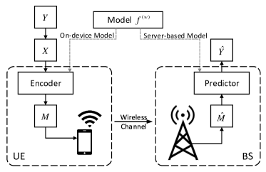
Figure 1: System model.

The performance of the learning model $f^{(W)}$ can be generally measured by a loss function $l(f^{(w)}(x),y)$ that calculates the distance between the model output and the target variable. We formally define the loss function as $l:\mathcal{W}\times\mathcal{Z}\to\mathbb{R}^{+}$. First, we consider the performance of standard distributed learning. We denote the loss function for a model output as standard loss $\tilde{l}\triangleq l(\tilde{y},y)$. Given the joint distribution of $p(x,y)$, the standard risk is taken on expectation as

$$L\triangleq\mathbb{E}_{p(w|z)}\mathbb{E}_{p(x,y)}\left[l(W,Z)\right]=\mathbb{E}_{p(w,z)}\left[l(W,Z)\right].$$ (2)

Note that $L$ is also taken expectation over $p(w|z)$, as we are evaluating the risk on all learned posterior instead of a specific hypothesis $w$.

In the context of wireless communication systems, the noisy channel may affect the learning algorithm and the feature transmission, thus deteriorating the model performance. Upon a specific channel realization with side information $s$, we denote the loss function for a distorted output as wireless loss $\hat{l}\triangleq l(\hat{y},y)$. We can take the expectation on the joint hypothesis and sample space given the side information as wireless risk

$$L(s)\triangleq\mathbb{E}_{q(w,z|s)}\left[l(W,Z)\right].$$ (3)

Therefore, the absolute difference between wireless risk and standard risk can be considered as the loss difference in the wireless environment. We denote the expectation on all channels as wireless risk discrepancy, which is given by

$$g(\mu,f)\triangleq\mathbb{E}_{\mu(s)}\left[|L(S)-L|\right].$$ (4)

The discrepancy can be viewed as an inverse of the model’s robustness to the imperfect wireless channel and its meaning is twofold. First, via the power of deep learning, we can learn a model minimizing the difference to obtain better robustness against distortion in wireless communication systems. Second, a small discrepancy indicates that the model allows for more channel perturbation while maintaining task performance, thus a relatively high transmission rate can be applied.

Conventional communication systems are designed for error-free transmission where the bit error rate (BER) is arbitrarily small. However, error-free transmission doesn’t necessarily align with the objectives of AI in a wireless scenario. The main goal of wireless distributed learning is to execute the task with sufficient precision, i.e., the accuracy in classification and the mean absolute error in regression. In the presence of wireless channel distortion, a task may still be completed successfully given the robustness of NNs. Therefore, we can transition from error-free to task-reliable transmission, exploiting the possible capacity gain in a wireless distributed learning system. To meet the task-reliable criterion, the system must ensure that the wireless risk discrepancy is negligible for the task’s successful execution despite transmission errors.

III Main Results

III-A Loss Function Analysis

To carry out information-theoretic analysis, we revisit the wireless risk discrepancy $g(\mu,f)$ in eq. 4, which measures the performance deterioration caused by the imperfect wireless channel. It can be viewed as the expected difference between distributions $q(w,z|s)$ and $p(w,z)$. Therefore, Kullback-Leibler (KL) divergence serves as a useful tool to measure the distance between $q$ and $p$. We leverage the Donsker-Varadhan variational representation of KL divergence in [8] as follows

$$D_{\text{KL}}(\pi\|\rho)=\sup_{F}\left\{\int_{\Omega}Fd\pi-\log\int_{\Omega}e^{F}d\rho\right\},$$ (5)

where the detailed lemma is presented in the appendix.

We further assume that the loss function $l(w,z)$ is $\sigma$-sub-Gaussian on distribution $p(w,z)$, which can be easily fulfilled by using a clipped loss function [9] [10]. Applying eq. 5 with $\pi=q(w,z|s)$, $\rho=p(w,z)$, and $F=\lambda l(w,z)$, we have the following theorem with the proof presented in the appendix.

Theorem 1

If the loss function $l(w,z)$ is $\sigma$-sub-Gaussian on distribution $p(w,z)$, then the wireless risk discrepancy is upper bounded by

$$g(\mu,f)\leq\sigma\sqrt{2I(W,Z;S)}\triangleq G.$$ (6)

Remark 1

In the context of wireless distributed learning, it is worth noting that the loss difference vanishes upon achieving error-free transmission, i.e., transmission rate $R<C$. Additionally, if the mutual information $I(W,Z;S)=0$, the the wireless risk discrepancy also becomes zero. It suggests that $(W,Z)$ is independent of side information $S$. In this scenario, the model is generalized to any wireless channel as analyzed in [11], thus accomplishing perfect inference in wireless distributed learning. However, the absolute independence is virtually unattainable. In practice, the learning algorithm can only find a model where the mutual information approaches zero.

Remark 2

Using the chain rule of mutual information, $I(W,Z;S)$ can be written as

$$I(W,Z;S)=I(Z;S)+I(W;S|Z),$$ (7)

and

$$I(W,Z;S)=I(W;S)+I(Z;S|W).$$ (8)

From eq. 7, it can be observed that the sample $Z$ consisting of input data $X$ and target $Y$ is independent of the wireless channel. Hence the first term $I(Z;S)=0$ and the mutual information can be reduced to $I(W,Z;S)=I(W;S|Z)$. The first term in eq. 8 represents the information of channel contained in the learned hypothesis. From the perspective of probably approximately correct (PAC) [11], a small $I(W;S)$ mitigates over-fitting on a specific channel and thus increases robustness against wireless channels. The second term can be further written as $I(Z;S|W)=I(Y;S|W,X)+I(X;S|W)$. In the classification problem, conditional mutual information $I(Y;S|W,X)$ becomes the cross-entropy between the wireless prediction $p(y|x,w,s)$ and the standard prediction $p(y|x,w)$. Hence, it can be considered as a distance between $\hat{y}$ and $\tilde{y}$.

Remark 3

The existing information-theoretic analysis based on IB [2] utilizes $I(X;T)$ to indirectly measure the robustness of NNs in edge inference. Unlike such an analysis on the data flow $X\to T$ [12], the derived upper bound $I(W,Z;S)$ quantifies the information of the wireless channel contained in the network and directly reveals the robustness against wireless distortion. Moreover, our measure is invariant to the choice of activation functions, since it is not directly influenced by hidden representations like $I(X;T)$.

III-B Channel Capacity Gain

The wireless risk discrepancy is a statistical measure averaged over the probability space and provides a general view. However, to delve deeper into the possible channel capacity gain benefited from the robustness, we pay special attention to each detailed event. Specifically, for an individual inference $(z,w,s)$, where $z$, $w$, and $s$ represent a particular sample, hypothesis, and channel, respectively, the difference between the actual wireless loss $\hat{l}(\hat{y}(x,w,s),y)$ and the true risk $L$ would possibly transcend the upper bound $G$ in Theorem 1. This deviation depends on the variability of the performance deterioration across different realizations, and deviations could occur due to variable samples, hypotheses, and channel conditions.

To better analyze the probabilistic nature of wireless distributed learning, we introduce the concept of task outage as in [13] and [14], which extends the outage in conventional communication systems towards the domain of wireless distributed learning. The concept of outage is the event that occurs whenever the capacity falls below a target rate $R$ [15]. However, given the robustness of NNs, lossy transmission is acceptable in wireless distributed learning as long as the performance is not severely affected. Therefore, we focus on the event that the instantaneous loss difference transcends the upper bound $G$ of the wireless risk discrepancy.

Definition 1

An individual wireless distributed inference $(z,w,s)$ with a transmission rate $R$ is considered as a task outage if

$$E=\mathbf{1}\left(\left|\hat{l}(\hat{y}_{R}(x,w,s),y)-L\right|\geq\sigma\sqrt{2I(W,Z;S)}\right),$$ (9)

where $\mathbf{1}(\cdot)$ is the indicator function, $\hat{y}_{R}(x,w,s)=f_{d}^{(w)}(\hat{m})$ is the output of the decoder, $\hat{m}$ is the received signal that is transmitted through wireless channel $s$ at rate $R$. The set of task outage can be written as $\mathcal{E}=\left\{\hat{l}:E=1\right\}$. Thus, the task outage probability is expressed as

$$p_{e}\triangleq\Pr\{E=1\}.$$ (10)

For a given $\epsilon<1$, the transmission rate R is task achievable if the task outage probability $p_{e}\leq\epsilon$.

In the conventional communication system, [16] defines $\epsilon$-achievable rate in the context of lossy transmission with error $\epsilon$. Given the task outage probability, we adopt this notion and apply it to the lossy transmission in wireless distributed learning.

Theorem 2

For a given $\epsilon<1$ and every $\delta>0$, the task achievable rate satisfies

$$R\leq\frac{1}{1-\epsilon}(C+\delta)\triangleq C_{s},$$ (11)

where $C=I(M;\hat{M})$ represents the Shannon’s channel capacity. We consider the maximum rate for robust wireless distributed inference as the channel capacity gain $C_{s}$.

Remark 4

It can be seen that the capacity gain falls back to Shannon’s channel capacity when $\epsilon=0$. In this scenario, the task outage would never occur, indicating that the wireless loss $\hat{l}$ must fall within a bounded region $[L-G,L+G]$. Since loss functions are usually unbounded or semi-bounded distributions, $p_{e}=0$ leads to $\hat{l}=\mathbb{E}[\hat{l}]$. Thus, it corresponds to the error-free transmission in Remark 1. On the contrary, the special case of $p_{e}=1$ is unattainable for common distributions in AI applications, thus the capacity gain could not be infinite.

Remark 5

We can observe from eq. 11 that the capacity gain increases with $p_{e}$. By exploring the definition of task outage probability $p_{e}=\Pr\left\{\left|\hat{l}-L\right|\geq G\right\}$, we perceive $p_{e}$ as a two-tailed probability of the distribution of $\hat{l}$. Several major factors contribute to the augmentation of probability.

• First, an increase in the variance of $\hat{l}$ or the transition to a heavy-tailed distribution may be noted. This indicates a high BER in communication, which arises from a high transmission rate. Therefore, with the increase of task achievable rate, a higher capacity gain could be obtained.

• Second, a small cut-off value $G$ also contributes to the increase of two-tailed probability. As analyzed in Remark 2, a small wireless risk discrepancy upper bound $G$ helps alleviate the over-fitting on a specific channel and thus enhances the model’s robustness against the impact of wireless channels. Therefore, a high channel capacity gain might be achieved despite the channel distortion.

• Third, the standard risk $L$ moving closer towards the tails of the distribution may increase $p_{e}$. As a result, the wireless risk discrepancy approaches the upper bound $G$ which implies the model’s capability of fully exploiting the intrinsic robustness in wireless distributed learning. Thus, a more substantial capacity gain could be possible.

IV Numerical Example

By deriving an information-theoretic upper bound for the performance deterioration, we shed light on how to exploit the channel capacity gain from the robustness in wireless distributed learning. The key challenge ahead is the calculation of $I(W,Z;S)$ in a practical setting. We address this issue by utilizing an NN-based model $f^{(W)}$ in wireless distributed learning as an example. As specified in Remark 2, we turn to estimate the conditional mutual information $I(W;S|Z)$ for convenience. It can be written as the expectation of the KL divergence between $p(w|s,z)$ and $p(w|z)$ as

$$I(W;S|Z)=E_{p(s,z)}\left[D_{\text{KL}}(p(w|s,z)\|p(w|z))\right].$$ (12)

The two probabilities could respectively serve as posterior and prior of the hypothesis given side information as evidence. Following the common assumption in deep learning theory, we assume both $p(w|z)=\mathcal{N}(w|\theta_{z},\Sigma_{z})$ and $p(w|s,z)=\mathcal{N}(w|\theta_{s,z},\Sigma_{s,z})$ are Gaussian distribution. The means $\theta_{z},\theta_{s,z}$ are the yielded hypotheses of the learning algorithm given the corresponding knowledge. Thus, the KL divergence term has a closed-form solution as

$$\begin{split}D_{\text{KL}}(p(w|s,z)\|p(w|z))=\frac{1}{2}\left[\log\frac{\det\Sigma_{s,z}}{\det\Sigma_{z}}-D\right.\\ \left.+\left(\theta_{s,z}-\theta_{z}\right)^{\top}\Sigma_{z}^{-1}\left(\theta_{s,z}-\theta_{z}\right)+\operatorname{tr}\left(\Sigma_{z}^{-1}\Sigma_{s,z}\right)\right],\end{split}$$ (13)

where $\det$ and $\operatorname{tr}$ represent the determinant and trace of a matrix, $D$ represents the dimension of hypothesis $w$, which is a constant for a specific model $f^{(W)}$. For simplicity, we further assume the covariance of prior and posterior are proportional, which is a common practice in PAC-Bayes analysis [17]. As a result, the logarithmic and trace terms in eq. 13 become constant and the conditional mutual information can be expressed as

$$I(W;S|Z)\propto E_{p(s,z)}\left[\left(\theta_{s,z}-\theta_{z}\right)^{\top}\Sigma_{z}^{-1}\left(\theta_{s,z}-\theta_{z}\right)\right].$$ (14)

Directly calculating the covariance $\Sigma_{z}$ on $p(w|z)$ is unachievable, so we resort to the bootstrapping method for approximation as [11]. In PAC-Bayes analysis, $p(w|z)=\mathbb{E}_{p(s)}\left[p(w|s,z)\right]$ is referred as prior when minimizing $D_{\text{KL}}(p(w|s,z)\|p(w|z)$. Thus, the prior covariance can be approximated using bootstrapping by

$$\Sigma_{z}\approx\frac{1}{K}\sum_{k=1}^{K}\left(\theta_{(s,z)_{k}}-\theta_{s,z}\right)\left(\theta_{(s,z)_{k}}-\theta_{s,z}\right)^{\top},$$ (15)

where $(s,z)_{k}$ is a bootstrap sampling set from space $\mathcal{S}\times\mathcal{Z}$ in the $k$-th experiment. During the training process of deep learning, it is prohibitive to learn hypothesis $\theta_{(s,z)_{k}}$ from $K$ bootstrapping samples. Therefore, we further utilize the influence function (IF) from robust statistic [18] to approximate the difference $\theta_{(s,z)_{k}}-\theta_{s,z}$.

Lemma 1 (Influence Function [19])

Assume in Poisson bootstrapping that the sampling weights denoted by $\boldsymbol{\xi}=(\xi_{1},\cdots,\xi_{n})^{\top}$ follows a binomial distribution $\xi_{i}\sim\text{Binomial}(n,\frac{1}{n})$ ($\lim_{n\to\infty}\text{Binomial}(n,\frac{1}{n})\to\text{Poisson}(1)$). Given new hypotheses $\hat{\theta}_{(s,z),\boldsymbol{\xi}}\triangleq\arg\min\frac{1}{n}\sum_{i=1}^{n}\xi_{i}\hat{l}_{i}(\theta)$ and $\hat{\theta}_{s,z}\triangleq\arg\min\frac{1}{n}\sum_{i=1}^{n}\hat{l}_{i}(\theta)$, the approximation of difference is defined by

$$\hat{\theta}_{(s,z),\boldsymbol{\xi}}-\hat{\theta}_{s,z}\approx\frac{1}{n}\sum_{i=1}^{n}(\xi_{i}-1)\psi_{i}=\frac{1}{n}\boldsymbol{\psi}^{\top}(\boldsymbol{\xi}-\boldsymbol{1}),$$ (16)

where $\psi_{i}=-\boldsymbol{H}_{\hat{\theta}_{s,z}}^{-1}\nabla_{\theta}\hat{l}_{i}(\hat{\theta}_{s,z})$ represents the IF, $\boldsymbol{\psi}=(\psi_{1},\cdots,\psi_{n})^{\top}$ represents the collection of IFs, and $\boldsymbol{H}_{\hat{\theta}_{s,z}}=\frac{1}{n}\sum_{i=1}^{n}\nabla_{\theta}^{2}\hat{l}_{i}(\hat{\theta}_{s,z})$ represents the Hessian matrix. As a result, the covariance can be approximated as

$$\Sigma_{z}\approx\frac{1}{K}\sum_{k=1}^{K}\left(\hat{\theta}_{(s,z),\boldsymbol{\xi}_{k}}-\hat{\theta}_{s,z}\right)\left(\hat{\theta}_{(s,z),\boldsymbol{\xi}_{k}}-\hat{\theta}_{s,z}\right)^{\top}\approx\frac{1}{n}\boldsymbol{F}_{\hat{\theta}_{s,z}}^{-1},$$ (17)

where $\boldsymbol{\xi}_{k}$ is the sampling weights in the $k$-th experiment and $\boldsymbol{F}_{\hat{\theta}_{s,z}}$ is the Fisher information matrix.

Now we are able to approximate the conditional mutual information in eq. 14 as

$$\begin{split}I(W;S|Z)&\propto n\mathbb{E}_{p(s,z)}\left[\left(\theta_{s,z}-\theta_{z}\right)^{\top}\boldsymbol{F}_{\hat{\theta}_{s,z}}^{-1}\left(\theta_{s,z}-\theta_{z}\right)\right]\\ &\approx n\left(\overline{\theta}_{s,z}-\theta_{z}\right)^{\top}\boldsymbol{F}_{\hat{\theta}_{s,z}}^{-1}\left(\overline{\theta}_{s,z}-\theta_{z}\right),\end{split}$$ (18)

where we employ quadratic mean $\overline{\theta}_{s,z}=\sqrt{\frac{1}{K}\sum_{k=1}^{K}\hat{\theta}_{(s,z),\boldsymbol{\xi}_{k}}^{2}}$ to better estimate $\theta_{s,z}$ in the expectation. In practice, we could pre-train a model in standard distributed learning to obtain $\theta_{z}$, and we denote $\Delta\theta=\overline{\theta}_{s,z}-\theta_{z}$. By expanding the Fisher information matrix, eq. 18 can be simplified as

$$\begin{split}I(W;S|Z)&\propto n\Delta\theta^{\top}\left[\frac{1}{T}\sum_{t=1}^{T}\nabla_{\theta}\hat{l}_{t}(\hat{\theta}_{s,z})\nabla_{\theta}\hat{l}_{t}(\hat{\theta}_{s,z})^{\top}\right]^{-1}\Delta\theta\\ &=\frac{n}{T}\sum_{t=1}^{T}\left[\Delta\theta^{\top}\nabla_{\theta}\hat{l}_{t}(\hat{\theta}_{s,z})\right]^{2}\triangleq\tilde{I}(W;S|Z),\end{split}$$ (19)

where $n$ denotes the number of samples and $T$ denotes the number of iterations to estimate Fisher information. The algorithm to efficiently approximate $\tilde{I}(W;S|Z)$ is summarized in Algorithm 1.

Algorithm 1 Efficient approximation of conditional mutual information $I(W;S|Z)$

0:  Number of samples $n$, number of batches $B$, number of estimation iterations $T$, average parameters $(\rho,K)$.

0:  Approximated $\tilde{I}(W;S|Z)$.

1:  Pre-train in standard distributed learning, $\theta_{z}\leftarrow p(w|z)$.

2:  for $t=1:B$ do

3:     Train in wireless distributed learning, calculate and store the gradient $\nabla l_{t}$.

4:     Back-propagation and update hypothesis $\hat{\theta}_{t}$.

5:     Apply moving average hypotheses over $K$ iterations $\overline{\theta}_{t}\leftarrow\sqrt{\rho\overline{\theta}_{t-1}^{2}+\frac{1-\rho}{K}\sum_{k=0}^{K}\hat{\theta}_{t-k}^{2}}$.

6:  end for

7:  $\Delta\theta\leftarrow\overline{\theta}_{B}-\theta_{z}$, $\Delta F\leftarrow 0$.

8:  for $t=1:T$ do

9:     $\Delta F_{t}\leftarrow\Delta F_{t-1}+(\Delta\theta^{\top}\nabla l_{t})^{2}$.

10:  end for

11:  $\tilde{I}(W;S|Z)\leftarrow\frac{n}{T}\Delta F_{T}$.

V Simulations

In this section, we implement a wireless distributed learning system for the classification problem to verify the interpretability of the proposed capacity gain in Section III. We employ a 6-layer CNN on a classic binary classification dataset of ASIRRA Cats & Dogs [20]. Specifically, the encoder $f_{e}^{(w)}$ and decoder $f_{d}^{(w)}$ consist of the model’s first three and final three layers, respectively. Regarding the wireless channel setting, we use the additive white Gaussian noise (AWGN) and Rayleigh channels. Moreover, we incorporate modulation to ensure compatibility with modern wireless communication systems.

First, we train the model under both standard and wireless distributed learning. We adopt existing differentiable quantization techniques to facilitate training using QPSK. The empirical risk $\hat{L}$ and $\hat{L}(s)$ are averaged on multiple training results. Furthermore, we calculate the average difference across multiple channel realizations to derive $\hat{g}(\mu,f)=\frac{1}{n}\sum_{i}\left|\hat{L}(s_{i})-L\right|$. Meanwhile, we approximate the upper bound $\hat{G}$ via Algorithm 1 and compute the task outage probability $p_{e}$. The outcomes are summarized in Table I, with the parenthesis indicating the power of channel noise. From the table, the actual wireless risk discrepancy is maintained within the theoretical upper bound across various channel conditions. Hence, it effectively validates the reliability of the theorem on the wireless risk discrepancy and the distributed learning system’s inherent robustness.

TABLE I: Comparison between loss difference and upper bound

Channel	$\hat{g}(\mu,f)$	$\hat{G}$	$p_{e}$
AWGN (5dB)	0.0556	0.0670	0.2777
AWGN (10dB)	0.0310	0.0621	0.2558
AWGN (15dB)	0.0278	0.0623	0.2557
Rayleigh (5dB)	0.0780	0.0895	0.2897
Rayleigh (10dB)	0.0501	0.0719	0.2766
Rayleigh (15dB)	0.0383	0.0622	0.2648

Additionally, we endeavor to illustrate the channel capacity gain resulting from the robustness in wireless distributed learning. Specifically, we perform the distributed inference task with a particular model over the wireless channel at various transmission rates, achieved by employing different modulation schemes (from BPSK to 64QAM). In Figure 2, we plot the performance curves with loss on the x-axis and rate on the y-axis for a clear presentation. According to Definition 1, we identify the complement of task outage set $\mathcal{E}^{c}$ as the task achievable region. In the simulation, the loss is an average on the dataset, it is valid to assert that the task outage probability remains below $p_{e}$ when $\left|\hat{l}-L\right|<G$.

From the figures, there exists a transmission rate $R$ with which the performance falls at the boundary of task achievable region. Therefore, a successful task can be accomplished by employing such a transmission rate. Notably, the rate $R$ surpasses the Shannon channel capacity $C$, thus corroborating the intrinsic robustness in wireless distributed learning. Furthermore, we compute the channel capacity gain $C_{s}$ in eq. 11 using the task outage probability $p_{e}$ from Table I. It can be seen from Figure 2 that the achievable rate $R$ falls below $C_{s}$, aligning with the proposed theorem.

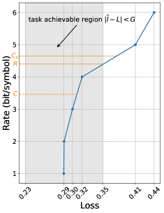
(a) AWGN channel.

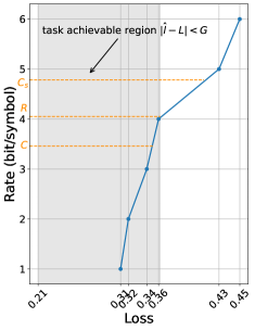
(b) Rayleigh channel.

Figure 2: The performance curves at different rates in AWGN and Rayleigh channels. The shadows denote the task achievable region.

VI Conclusion

In this paper, we have presented an information-theoretic analysis of the robustness within wireless distributed learning and its implications for achieving channel capacity gain. By leveraging information theory, we derived an upper bound in terms of mutual information on the performance deterioration due to the wireless fading. In contrast to the bit-level metric, we defined task outage based on the upper bound as a metric for successful inference. Thereby, we characterized the maximum achievable rate in wireless distributed learning and the channel capacity gains benefited from robustness. We further proposed an efficient algorithm to estimate the upper bound in practice. The robustness in wireless distributed learning is validated through numerical experiments.

References

- [1] E. Bourtsoulatze, D. B. Kurka, and D. Gündüz, “Deep joint source-channel coding for wireless image transmission,” IEEE Trans. Cogn. Commun. Netw., vol. 5, no. 3, pp. 567–579, Sep. 2019.
- [2] J. Shao, Y. Mao, and J. Zhang, “Learning task-oriented communication for edge inference: An information bottleneck approach,” IEEE J. Sel. Areas Commun., vol. 40, no. 1, pp. 197–211, Jan. 2022.
- [3] H. Xie, Z. Qin, G. Y. Li, and B.-H. Juang, “Deep learning enabled semantic communication systems,” IEEE Trans. Signal Process., vol. 69, pp. 2663–2675, 2021.
- [4] J. Bao, P. Basu, M. Dean, C. Partridge, A. Swami, W. Leland, and J. A. Hendler, “Towards a theory of semantic communication,” in Proc. IEEE Netw. Sci. Workshop, Jun. 2011, pp. 110–117.
- [5] L. Xia, Y. Sun, D. Niyato, X. Li, and M. A. Imran, “Joint user association and bandwidth allocation in semantic communication networks,” IEEE Trans. Veh. Technol., to appear.
- [6] J. Liu, W. Zhang, and H. V. Poor, “A rate-distortion framework for characterizing semantic information,” in Proc. IEEE Int. Symp. Inf. Theory (ISIT), Jul. 2021, pp. 2894–2899.
- [7] Y. Shao, Q. Cao, and D. Gündüz, “A theory of semantic communication,” arXiv preprint arXiv:2212.01485, 2022.
- [8] R. M. Gray, Entropy and information theory. Berlin, Germany: Springer Science & Business Media, 2011.
- [9] P. Rigollet and J.-C. Hütter, “High-dimensional statistics,” arXiv preprint arXiv:2310.19244, 2023.
- [10] A. Xu and M. Raginsky, “Information-theoretic analysis of generalization capability of learning algorithms,” in Proc. Adv. Neural Inf Process. Syst. (NIPS), Dec. 2017, pp. 2521–2530.
- [11] Z. Wang, S.-L. Huang, E. E. Kuruoglu, J. Sun, X. Chen, and Y. Zheng, “PAC-bayes information bottleneck,” in Proc. Int. Conf. Learn. Represent. (ICLR), Apr. 2022.
- [12] Z. Goldfeld, E. Van Den Berg, K. Greenewald, I. Melnyk, N. Nguyen, B. Kingsbury, and Y. Polyanskiy, “Estimating information flow in deep neural networks,” in Proc. Int. Conf. Mach. Learn. (ICML). Jun. 2019, pp. 2299–2308.
- [13] G. Zhang, Q. Hu, Y. Cai, and G. Yu, “Scan: Semantic communication with adaptive channel feedback,” arXiv preprint arXiv:2306.15534, 2023.
- [14] T. M. Getu, W. Saad, G. Kaddoum, and M. Bennis, “Performance limits of a deep learning-enabled text semantic communication under interference,” arXiv preprint arXiv:2302.14702, 2023.
- [15] D. Tse and P. Viswanath, Fundamentals of Wireless Communication. Cambridge, U.K.: Cambridge Univ. Press, 2005.
- [16] S. Verdu and T. S. Han, “A general formula for channel capacity,” IEEE Trans. Inf. Theory, vol. 40, no. 4, pp. 1147–1157, 1994.
- [17] G. K. Dziugaite and D. M. Roy, “Data-dependent pac-bayes priors via differential privacy,” in Proc. Adv. Neural Inf Process. Syst. (NIPS), Dec. 2018, pp.8440–8450.
- [18] P. W. Koh and P. Liang, “Understanding black-box predictions via influence functions,” in Proc. 34th Int. Conf. Mach. Learn. (ICML), Aug. 2017, pp. 1885–1894.
- [19] R. D. Cook and S. Weisberg, Residuals and Influence in Regression. New York, NY, USA: Chapman and Hall, 1982.
- [20] W. Cukierski, “Dogs vs. cats,” 2013. [Online]. Available: https://kaggle.com/competitions/dogs-vs-cats