The Hot Circum-Galactic Medium in the eROSITA All Sky Survey

Abstract

Context. The circum-galactic medium (CGM) provides the material for galaxy formation and influences galaxy evolution. The hot CGM ($T>10^{6}K$) is poorly detected around Milky-Way-mass (MW-mass, $\log M_{*}=10.5-11.0$) and M31-mass ($\log M_{*}=11.0-11.25$) galaxies, due to its low surface brightness.

Aims. We aim to detect the X-ray emission from the hot CGM around MW-mass and M31-mass galaxies, measure the X-ray surface brightness profile of the hot CGM.

Methods. We apply a stacking technique to gain enough statistics to detect the hot CGM. We use the X-ray data from the first four Spectrum Roentgen Gamma (SRG)/eROSITA all-sky surveys (eRASS:4). We discuss how the satellite galaxies could bias the stacking and carefully build the central galaxy samples. First, based on the SDSS spectroscopic survey and halo-based group finder algorithm, we select central galaxies with $z_{\rm spec}<0.2$ and stellar mass $10.0<\log(M_{*})<11.5$ (85,222 galaxies), or halo mass $11.5<\log(M_{\rm 200m})<14.0$ (125,512 galaxies); these two samples are the default samples used to measure the X-ray surface brightness profiles. Then, to obtain higher statistics at lower mass, we define an isolated galaxy selection criteria and select isolated galaxies from the ninth data release of the DESI Legacy survey (LS DR9, photometric) with stellar mass $9.5<\log(M_{*})<11.5$ and $z_{\rm phot}<0.4$ (213,514 galaxies). By stacking the X-ray emission around galaxies, we obtain the average X-ray surface brightness profiles. We mask the detected X-ray point sources and carefully model the X-ray emission from the unresolved active galactic nuclei (AGN) and X-ray binaries (XRB) to obtain the X-ray emission from the hot CGM.

Results. The X-ray surface brightness profiles are measured for $\log(M_{*})>10.0$ or $\log(M_{\rm 200m})>11.5$ central galaxies, and $\log(M_{*})>9.5$ isolated galaxies. We detect the X-ray emission around MW-mass and more massive central galaxies extending up to the virial radius ($R_{\rm vir}$). The signal-to-noise ratio of the extended emission around M31-mass (MW-mass) galaxy is about $12.3\sigma$ ($8.1\sigma$) within $R_{\rm vir}$, and is about $4.5\sigma$ ($3.1\sigma$) within $(0.5-1)R_{\rm vir}$. We subtract the emission from the unresolved X-ray sources and use the $\beta$ model to describe the X-ray surface brightness ($S_{\rm X}$) profiles of the hot CGM. We obtain a central surface brightness of $S_{\rm X,0}\approx 3.1\times 10^{35}\rm erg/s/kpc^{2}$ and $\beta\approx 0.42$ for MW-mass galaxy, $S_{\rm X,0}\approx 1.3\times 10^{36}\rm erg/s/kpc^{2}$ and $\beta\approx 0.37$ for M31-mass galaxy, $S_{\rm X,0}\approx 6.3\times 10^{36}\rm erg/s/kpc^{2}$ and $\beta\approx 0.35$ for galaxy with $\log(M_{*})=11.25-11.5$. We estimate the baryon budget of the hot CGM and obtain a value lower than the $\Lambda CDM$ cosmology predicted. Though the isolated galaxies are located in a more sparse environment than the central galaxies, we do not detect differences in their surface brightness profiles.

Conclusions. We measure with high significance the extended X-ray emission out to $R_{\rm vir}$ around a population of MW-mass and more massive central galaxies. Our results set a firm footing for the presence of a hot CGM around such galaxies. These measurements constitute a new benchmark for galaxy evolution models and possible implementations of feedback processes therein.

1 Introduction

The circum-galactic medium (CGM) is the gas reservoir of a galaxy, thus closely related to galaxy evolution processes. Understanding the properties of CGM is essential to the study of galaxy formation and evolution, for example, the strength of the feedback processes and how they modulate the star formation and gas activity (Tumlinson et al., 2017; Naab & Ostriker, 2017; Truong et al., 2020; Oppenheimer et al., 2021; Truong et al., 2021). The observed CGM has multiple phases. Its temperature ranges from $<10^{4}$ K to $>10^{6}$ K. The cold ($T<10^{4}K$), cool ($T=10^{4}-10^{5}K$) and warm ($T=10^{5}-10^{6}K$) phases of CGM have been well studied (Prochaska et al., 2011; Tumlinson et al., 2011; Putman et al., 2012; Werk et al., 2014, 2016; Prochaska et al., 2017). The next vital target is a complete picture of the relationship between the galaxy and its hot phase of the CGM.

The hot ($T>10^{6}K$) phase of the CGM is the dominant mass component of the CGM baryon budget (Tumlinson et al., 2017). This hot CGM can be heated and shaped by the gravitational accretion shock and feedback processes, for example, AGN and stellar feedback. It emits X-rays via collisionally ionized gas emission lines and bremsstrahlung. Pointed observations using Chandra or XMM-Newton revealed the hot gas properties of a few nearby galaxies within a distance of 50 Mpc(Strickland et al., 2004; Tüllmann et al., 2006; Wang, 2010; Dai et al., 2012; Li & Wang, 2013; Bogdán et al., 2013, 2015; Anderson et al., 2016; Li et al., 2016). The hot gas surveys of Chandra and XMM-Newton focus on the inner hot CGM, or ‘corona,’ with scale-heights of about 1-30 kpc (median of 5 kpc), where feedback processes dominate over gravitation. With their spatial resolution, XMM-Newton and especially Chandra resolve the stellar structures distributed in the disk of nearby galaxies. Still, the number of galaxies around which we detect the extended emission of the CGM is limited in number and extension.

For the outer hot CGM, where virialized gas dominates, to heat the gas to X-ray emitting temperature over the radiation cooling curve through gravitation, $M_{\rm halo}$ needs to be high enough (typically ¿$10^{12.7}M_{\odot}$). This corresponds to massive galaxies with about $M_{*}>10^{11}M_{\odot}$ (Kereš et al., 2009b, a; van de Voort et al., 2016; Li et al., 2016; Liu et al., 2022). For these reasons, although the hot gas in galaxy groups and clusters has been detected and studied well (Pratt et al., 2019; Walker et al., 2019), very few detections of the outer hot CGM (out to 70 kpc) from galaxies have been reported (Dai et al., 2012; Bogdán et al., 2013, 2015; Anderson et al., 2016; Li et al., 2016; Das et al., 2020).

To chart the CGM outer emission beyond the local Universe, we use stacking techniques to detect its faint emission, provided large enough volumes are surveyed. By stacking about 250,000 ‘locally brightest galaxies’ selected from the Sloan Digital Sky Survey (SDSS) using data from ROSAT All-Sky Survey, Anderson et al. (2015) detected hot gas emission around $M_{*}>10^{10.8}M_{\odot}$ galaxies. Besides X-ray observations, studies of the CGM with the thermal Sunyaev–Zeldovich (tSZ) effect have progressed in the last years, for example, the Atacama Cosmology Telescope (Aiola et al., 2020). The thermal energy density profile of the CGM is measured around $M_{*}>10^{10.6}M_{\odot}$ galaxies by cross-correlating and stacking the WISE and SuperCOSmos photometric redshift galaxy sample with ACT and Planck (Bilicki et al., 2016; Das et al., 2023).

X-ray stacking experiments are now dramatically progressing thanks to the extended ROentgen survey with an Imaging Telescope Array (eROSITA) on board the Spektrum Roentgen Gamma (SRG) orbital observatory. Launched in 2019, eROSITA is a sensitive X-ray telescope performing an all-sky survey with a wide-field focusing telescope (Merloni et al., 2012; Predehl et al., 2021; Sunyaev et al., 2021; Merloni et al., 2024). The sensitivity of eROSITA is maximal in the soft energy band, namely below 2.3 keV, which makes it suitable for studying the million-degrees hot CGM emission. Recently, with eROSITA and its PV/eFEDS observations covering 140 square degrees, Comparat et al. (2022) stacked $\sim$16,000 central galaxies selected from the GAMA spectroscopic galaxy survey; later, Chadayammuri et al. (2022) stacked $\sim$1,600 massive galaxies selected from SDSS in the same eFEDS field. Both works detected and measured weak X-ray emission from the outer CGM of those galaxies by stacking star-forming and quiescent galaxies separately. Still, the difference in the sample selection led to different interpretations of the results.

Four of the planned eight all-sky surveys (eROSITA all-sky survey, eRASS:4), each lasting six months, have been completed. The X-ray data currently available for CGM stacking studies is about 40 times larger than what was available for the eFEDS region (100 times more area covered with about 40% the exposure time). In this work and the accompanying papers, we apply the stacking technique to the eRASS:4 X-ray data and a set of different galaxy samples of high statistical completeness. In this paper, we study the X-ray surface brightness profile of the hot CGM. In the companion papers based on the same samples, we investigate (i) the scaling relations between X-ray luminosity, stellar mass, and halo mass (Zhang et al. 2024b, submitted); (ii) the trends as a function of specific star formation rate (Zhang et al., in preparation); (iii) the possible dependence of the hot CGM emission on azimuth angle (Zhang et al., in preparation).

We organize this paper as follows. We introduce the eROSITA X-ray data reduction and stacking method in Sect. 2. We define the galaxy samples in Sect. 3. We describe the models (AGN, XRB) and mock galaxy catalogs in Sect. 4. We present the average X-ray surface brightness profiles of the galaxy population in Sect. 5. We show the X-ray surface brightness profiles of isolated and central galaxies and their hot CGM in Sect. 6 and Sect. 7. We estimate the baryon budget for MW-mass and more massive galaxies in Sect. 8. Throughout, we use Planck Collaboration et al. (2020) cosmological parameters: $H_{0}=67.74\ \rm km/s/Mpc$ and $\Omega_{\rm m}=0.3089$. The $\log$ in this work means $\log_{10}$.

2 X-ray data reduction and stacking

In this section, we describe the reduction of the X-ray data (Sect.  2.1), the stacking method (Sect. 2.2), the calculation of the uncertainties (Sect.  2.3), the PSF models (Sect.  2.4), and the $\beta$ model used (Sect. 2.5).

2.1 X-ray data reduction

We use the eRASS:4 data in the western Galactic hemisphere ($179.9442^{\circ}<l\leqslant 359.9442^{\circ}$). For the analysis, we use the eROSITA Science Analysis Software System (eSASS; Brunner et al., 2022) data products (version 020) of eRASS:4 (Merloni et al., 2024). We stage the data in 2439 overlapping sky tiles covering $3.6^{\circ}\times 3.6^{\circ}$. For each sky tile, we have energy-calibrated event files, vignetting corrected mean exposure map in three bands (0.3-0.6 keV, 0.6-1.0 keV, 1.0-2.0 keV), and a catalog of detected sources in the 0.2-2.3 keV band down to low detection likelihood (DET_LIKE_0$>5$). We use the default flag that removes events that are either singly corrupt or are part of a corrupted frame. We keep all patterns of events. eROSITA has seven telescope modules (TMs); two TMs suffer from light leaks (TM5 and 7; Predehl et al., 2021) and have a higher background. We use all TMs data in this work. The vignetted exposure time of eRASS:4, in the 0.5-2 keV band, ranges from 300s to 10,000s, with a median value of 550s.

The interstellar gas of the Milky Way or nearby dwarf galaxies absorbs soft X-ray photons. We focus here on the extra-galactic sky to measure the faint hot CGM of galaxies. The neutral atomic hydrogen column density ($N_{\rm H}$) is a solid absorption indicator. We mask the sky area with $N_{\rm H}>10^{21}\rm cm^{-2}$, referring to the full-sky HI4PI column density map (HI4PI Collaboration et al., 2016). The extinction from the dust in the Milky Way causes the reddening of the optical photometry of galaxies and affects the quality of galaxy parameter estimation. Using the thermal dust emission model from Planck observation (Planck Collaboration et al., 2014), we keep the sky area with $E(B-V)<0.1$.

The source detection pipeline of eROSITA may fail around bright sources (for example, Sco X-1 and Virgo cluster), and the background caused by them is high (Merloni et al., 2024). We mask these X-ray overdense regions where potentially spurious sources cluster (see the masking procedure from Merloni et al. (2024)). After applying the masks detailed above, there remains about 11,000 deg² covered by X-ray observations ($A_{\rm X}$).

2.2 Stacking method

We adopt the stacking method of Comparat et al. (2022). We calculate the physical (proper) distance between events and galaxies ($R_{\rm kpc}$) according to the redshift ($z$) of the galaxy and angular separation ($R_{\rm rad}$). We create an event cube for each galaxy in the sample by retrieving events within 3 Mpc of each galaxy ($\rm CUBE_{event}$). Each event cube contains the information of the position $(RA,DEC)$, the angular separation and physical distance ($R_{\rm rad}$ and $R_{\rm kpc}$) to the associated galaxy, the exposure time $t_{\rm exp}$, the observed energy $E_{\rm obs}$, the corresponding rest frame energy $E_{\rm rest}=E_{\rm obs}\times(1+z)$, the effective area $A_{\rm eff}$ of the telescope at the observed energy of each event.

We mask sources detected by eRASS:4, the masking radius of each source is conservatively set to $1.4\times R_{\rm src}$ to avoid residual emission, where $R_{\rm src}$ is the source radius derived from srctool (see appendix A of Comparat et al., 2023). In each cube, we assign a mask flag to each event.

The area loss due to masking needs to be corrected when calculating X-ray surface brightness. To do so, we generate randomly distributed points ($P_{\rm rd}$) over the sky with a density of $3000\ \rm deg^{-2}$. We add a flag of masked or unmasked to $P_{\rm rd}$ according to the same positions and radii as the real detected sources. We retrieve $P_{\rm rd}$ around each galaxy as described above to create a random point cube ($\rm CUBE_{prd}$).

Stacking a galaxy sample consists of merging the data cubes for all galaxies in the sample and extracting a summary statistic. Each event is assigned a weight:

$$W_{e}=E_{\rm obs}\frac{1}{t_{\rm exp}}\frac{f_{\rm nh}A_{\rm corr}\,4\pi D_{L}^{2}}{A_{\rm eff}}\ [\rm ergs^{-1}Mpc^{2}cm^{-2}],$$ (1)

where $D_{\rm L}$ is the luminosity distance to the galaxy, $A_{\rm corr}$ is the correction factor of area derived by merging the $\rm CUBE_{prd}$ of galaxies and take the ratio between numbers of all $P_{\rm rd}$ and unmasked $P_{\rm rd}$, as a function of $R_{\rm rad}$ or $R_{\rm kpc}$ to a galaxy. $A_{\rm corr}$ decreases with $R_{\rm kpc}$ and is about 1.2 at the center and 1.1 at the outskirt when masking X-ray sources. Without masking applied, it is 1. $f_{\rm nh}$ is a function that corrects as a function of the $E_{\rm obs}$ and $N_{\rm H}$ (taken from H14PI (HI4PI Collaboration et al., 2016)) the effects of absorption on the soft X-ray photons. We obtain it using the TBABS absorption model (Wilms et al., 2000).

The X-ray surface brightness profile around galaxies ($S_{\rm X,gal}$) is calculated by selecting the events located in radial bins ($\rm r_{0}<R_{kpc}<r_{1}$) and summing them up,

$$S_{\rm X,gal}=\Sigma_{r_{0}}^{r_{1}}\frac{W_{\rm e}}{A_{\rm shell}N_{\rm g}}\ [\rm erg/s/kpc^{2}],$$ (2)

where $A_{\rm shell}$ is the area of each radial bin and $N_{\rm g}$ is the number of galaxies stacked.

The background surface brightness ($S_{\rm X,bg}$) is taken as the minimum value of $S_{\rm X,gal}$ ($S_{\rm X,min}$) beyond $R_{\rm 500c}$. We detail the background estimation procedure validation in Appendix. A.

We use the energy bin $0.5-2$ keV (in rest frame) to calculate the X-ray surface brightness.

2.3 Uncertainty calculation

We estimate the uncertainty on $S_{\rm X,gal}$ with the quadratic sum of the Poisson error and the stacking uncertainty, which we estimate with the Jackknife re-sampling.

We estimate the Poisson error of the X-ray surface brightness profile by $1/\sqrt{n_{\rm total}}$, where $n_{\rm total}$ is the total event numbers in the corresponding radial bin. We estimate the Poisson error of background by $1/\sqrt{n_{\rm bg}}$, where $n_{\rm bg}$ is the total event number in the annulus used to estimate the background.

We use the Jackknife re-sampling method (Andrae, 2010; McIntosh, 2016) to compute the uncertainties from the stacking process. The Jackknife re-sampling logic is to select a subsample from the parent sample (re-sampling) and repeat enough times to estimate the scatter induced by outliers in the parent sample. The Jackknife re-sampling estimates the X-ray property variation of the stacked galaxy population. It allows one to assess, for example, if there is a large discrepancy of the X-ray property in the galaxy population or if the stacking result reflects the general property of the stacked galaxy sample.

In this work, we apply the Jackknife re-sampling in the following way: for one galaxy sample containing $N_{\rm gal}$ galaxies, we randomly select $90\%N_{\rm gal}$ galaxies from the sample, we stack the $90\%N_{\rm gal}$ galaxies and obtain the average $S_{\rm X,gal}$ of these $90\%N_{\rm gal}$ galaxies. We repeat the above procedure 200 times and retrieve the standard deviation of $S_{\rm X,gal}$ as the stacking uncertainty.

For reference, the uncertainties in our study are dominated by the stacking uncertainties, as the event number is significant. Therefore, the uncertainty of the $S_{\rm X,gal}$ of specific galaxy samples after masking detected X-ray sources might be smaller than the uncertainty of the $S_{\rm X,gal}$ without masking, even though the latter has lower Poisson error; this is because the X-ray luminosity variation of the galaxy sample is minor after masking bright X-ray sources.

2.4 PSF model

We use the eROSITA point spread function (PSF) model from Sanders et al. (in preparation; also, Merloni et al. (2024)). The PSF is on an angular scale, and we use the redshifts of galaxies to transfer it to the physical scale (kpc). We average the PSF profiles on the physical scales of galaxies in one sample and take it as the PSF convolved by the redshift distribution of the sample. We scale the mean PSF profile to the central value of the measured surface brightness profile for each stacking experiment. By comparing the X-ray surface brightness profile to the redshift-convolved mean PSF profile, we gauge the extension of the X-ray emission.

2.5 $\beta$ model and fitting procedure

We use the $\beta$ model (Cavaliere & Fusco-Femiano, 1976) to describe the X-ray profiles of the hot CGM. By assuming the X-ray emissivity of the hot CGM is a constant within the virial radius, the projected X-ray profile of the hot CGM with $\beta$ model reads

$$S_{\rm X,\beta}=S_{\rm X,0}\left[1+\left(\frac{r}{r_{\rm c}}\right)^{2}\right]^{-3\beta+\frac{1}{2}}\ [\rm erg/s/kpc^{2}],$$ (3)

where $S_{\rm X,0}$ is the X-ray surface brightness at the galaxy center, $r$ is the distance to the center, $r_{c}$ is the core radius. We convolve the $\beta$ profile with the PSF described in Sect. 2.4 and build the likelihood function. We estimate one group of the best parameters using the maximum likelihood method. We then run the Markov Chain Monte Carlo (MCMC) chain, starting with the parameters with large enough walkers and steps to estimate the best-fit parameters and their uncertainties. We take the best-fit value as the median value of the possible parameters from MCMC and the value at 16% and 84% of the possible parameters from MCMC as the $1\sigma$ uncertainties (Hogg et al., 2010).

3 Galaxy samples selection

We build galaxy samples based on two criteria: (i) its completeness (¿90%) to reduce the selection effects, and (ii) its size, where the larger, the better.

In this section, we calculate the maximum redshift limited by the PSF of eROSITA and the required galaxy survey depth to build a complete galaxy sample (Sect. 3.1). Based on the two criteria above, we compare galaxy surveys in Sect. 3.2 and introduce the two galaxy catalogs we will use (SDSS DR7 spectroscopic galaxy catalog and LS DR9 photometric galaxy catalog, Sect. 3.3). We discuss the connection of galaxy and dark matter halos in Sect. 3.4 and how the presence of satellite galaxy in the sample could bias the stacking result (Sect. 3.5). To minimize such bias, we finally define a central galaxy sample based on the SDSS spectroscopic galaxy survey (Sect. 3.6) and an isolated galaxy sample based on LS DR9 photometric galaxy catalog (Sect. 3.7).

3.1 Considerations on the maximum redshift and galaxy survey depth

Table 1: Constraints on the maximum redshifts of galaxies at different stellar masses to achieve $>95\%$ completeness.

log10(M∗)	log10(Mh)	Rh	$z_{\rm 2\times PSF}$	$z_{\rm 3\times PSF}$	$r_{AB,\rm 2\times PSF}$	$r_{AB,\rm 3\times PSF}$	$z_{\rm r_{AB}=17.77}$
[$M_{\odot}$]	[$M_{\odot}$]	[kpc]
9	11.0	82	0.07	0.04	19.5	18.5	¡0.02
9.5	11.3	102	0.09	0.06	19.4	18.8	0.04
10	11.6	131	0.12	0.075	19.2	18.1	0.06
10.5	12.0	178	0.17	0.10	19.1	17.8	0.1
10.75	12.2	210	0.21	0.13	19.1	17.9	0.12
11.0	12.7	295	0.33	0.19	19.4	18.3	0.15
11.25	13.3	480	0.91	0.37	19.3	19.4	0.19
11.5	14.3	950	¿1	¿1	19.2	19.2	0.25

To resolve the extended hot CGM, the PSF of eROSITA limits the maximum redshift up to which we should stack galaxies. With the stellar-to-halo mass relation from Moster et al. (2013), we infer the average dark matter halo mass and virial radius for a galaxy of a given stellar mass. We convert the virial radius to angular scale using the angular diameter distance as a function of redshift (Hogg, 1999). As a reference, we take the size of the eROSITA PSF as $\theta=30"$ (Sanders et al. in preparation, Merloni et al. (2024)) and calculate at which redshift the virial radius of the halo hosting the galaxy is equal to two and three times this value (i.e. $1^{\prime}$ and $1.5^{\prime}$), as listed in Table 1. For example, galaxies with $\log(M_{*})=10.75$ (similar to the Milky Way) have a resolved virial radius with two (three) eROSITA PSF up to $z=0.21$ ($z=0.13$). We then estimate the galaxy survey depth to ensure the galaxy sample’s completeness is higher than 95% (we take r-band magnitude $r_{\rm AB}$ to evaluate). For example, to resolve the virial halo of $\log(M_{*})=10.75$ galaxies with two (three) eROSITA PSF, the galaxy survey needs to be deeper than $r_{\rm AB}=19.1(17.9)$.

By stacking samples to $z_{\rm 2\times PSF}$, we obtain higher statistics to measure the luminosity of the CGM, and the survey depth should be more profound than $r_{\rm AB}=19.1$. Stacking samples to $z_{\rm 3\times PSF}$, we obtain a better resolution to measure the surface brightness profile of the CGM, and the survey depth can be shallower ($r_{\rm AB}=17.9$).

3.2 Choice of the galaxy sample

Table 2: Comparison of the galaxy catalog candidates.

Survey	$A_{\rm west}$ (deg2)	Magnitude cut	$N_{\rm gal}$	redshift	Reference
SDSS (DR7)	4010	r¡17.77	382428	spectroscopic	Strauss et al. (2002)
GAMA (DR4)	180	r¡19.8	58816	spectroscopic	Driver et al. (2022)
2MPZ	19450	$K_{s}$¡13.9	136005	photometric	Bilicki et al. (2014)
DESI Legacy (DR9)	9340	r¡23.4	2387058	photometric	Dey et al. (2019)

There are numerous photometric and spectroscopic redshift surveys covering the extra-galactic sky. To name a few, we have 2MASS, VHS, WISE, SDSS, skymapper, GAMA, DES, KIDS, DESI Legacy surveys (Skrutskie et al., 2006; Wright et al., 2010; McMahon et al., 2013; Almeida et al., 2023; Driver et al., 2022; Dey et al., 2019; Abbott et al., 2018; Onken et al., 2019; Bilicki et al., 2021). To make full use of the X-ray data at our disposal in the western Galactic hemisphere, we are interested in the catalogs with wide area coverage rather than depth, i.e., we do not consider deep fields like HUDF, CDFS, COSMOS (Beckwith et al., 2006; Hsu et al., 2014; Laigle et al., 2016). In Table 2, we list the information of some galaxy catalog candidates for this work.

The spectroscopic surveys provide more precise measurements of redshift, stellar population, and classification of galaxies. The GAMA survey, which has completeness above 95% for r${}_{AB}<19.8$, allows for a stacking to $z_{\rm 2\times PSF}$. However, the overlap area of its footprint with the western Galactic hemisphere is only 180 deg², which limits the galaxy sample size and statistics. The SDSS DR7 galaxy sample extends to $r_{\rm AB}<17.77$, with about 4010 square degrees of overlap to the western Galactic hemisphere. This survey provides enough statistics to study the CGM around galaxies within $z=0.2$. We take it to build the galaxy samples to explore the surface brightness profile of the CGM. Until 4MOST and DESI measure spectroscopic redshift for bright galaxies ($r_{AB}<20$) over all of eROSITA’s extra-galactic sky, to strive for large area and completeness, one needs to rely on photometric surveys (DESI Collaboration et al., 2016; de Jong et al., 2019; Finoguenov et al., 2019).

The 2MASS photometric redshift survey (2MPZ) covers the whole sky but is limited to the brightest galaxies due to its shallow depth (Bilicki et al., 2014). The deeper surveys, such as the Hyper Suprime-Cam Subaru Strategic Program (HSC-SSP), cover a smaller area ($\sim$1,500 square degrees up to now; e.g. Aihara et al., 2018). Currently, the most adequate photometric survey with sufficient depth ($r_{\rm AB}\sim$23.4) and coverage (9,340 deg² within the western Galactic hemisphere) is the DESI legacy survey ninth data release (LS DR9, Dey et al., 2019). We take it to build the galaxy sample out to $z_{\rm 2\times PSF}$ and down to $\log(M_{*})=9.5$, which provides the best statistics to measure the X-ray luminosity of the CGM. The photometric redshift and stellar masses in LS DR9 are available (Zou et al., 2019), as well as a special treatment for galaxies with a large extent on the sky available in the 2020 version of the Siena Galaxy Atlas (SGA-2020; Moustakas et al., 2023). In the longer term, Rubin and Euclid observatories will be an excellent resource with exquisite depth and complete coverage of the southern hemisphere (Ivezić et al., 2019; Laureijs et al., 2011).

Table 3: Description of the galaxy samples.

$\rm log_{10}(M_{*}/M_{\odot})$		$M_{\rm*,med}/M_{\odot}$	redshift			FULLspec	CEN	SAT
min	max		min	max	med	$N_{g}$	$N_{g}$	$N_{g}$
10.0	10.5	$1.8\times 10^{10}$	0.01	0.06	0.05	11922	7956	3966
10.5	11.0	$5.5\times 10^{10}$	0.02	0.10	0.08	45248	30825	14423
11.0	11.25	$1.3\times 10^{11}$	0.02	0.15	0.12	34046	26099	7947
11.25	11.5	$2.2\times 10^{11}$	0.03	0.19	0.15	24098	20342	3756

$\rm log_{10}(M_{*}/M_{\odot})$		$M_{\rm*,med}/M_{\odot}$	redshift			FULLphot	Isolated
min	max		min	max	med	$N_{g}$	$N_{g}$
9.5	10.0	$5.5\times 10^{9}$	0.01	0.09	0.07	95698	24280
10.0	10.5	$1.8\times 10^{10}$	0.01	0.12	0.10	214286	50137
10.5	11.0	$5.5\times 10^{10}$	0.02	0.17	0.14	415627	70348
11.0	11.25	$1.3\times 10^{11}$	0.02	0.33	0.28	627757	50766
11.25	11.5	$2.2\times 10^{11}$	0.03	0.40	0.35	324541	17983

$\rm log_{10}(M_{\rm 200m}/M_{\odot})$		$M_{\rm 200m,med}/M_{\odot}$	redshift			CENhalo
min	max		min	max	med	$N_{g}$
11.5	12.0	$5.5\times 10^{11}$	0.01	0.08	0.06	25368
12.0	12.5	$1.7\times 10^{12}$	0.02	0.13	0.09	41301
12.5	13.0	$5.0\times 10^{12}$	0.02	0.16	0.12	30740
13.0	13.5	$1.6\times 10^{13}$	0.03	0.20	0.14	19889
13.5	14.0	$4.8\times 10^{13}$	0.03	0.20	0.16	8214

3.3 FULL samples built from the SDSS DR7 and LS DR9 galaxy catalogs

3.3.1 SDSS DR7

We consider the galaxy catalog based on the SDSS Main Galaxy Sample (MGS) (Strauss et al., 2002; Abazajian et al., 2009). It covers 9,380 $\rm deg^{2}$ of the sky and overlaps with eROSITA-DE observations on about 4,010 square degrees. Based on the New York University Value-Added Galaxy Catalog (NYU-VAGC) from Blanton et al. (2005), a galaxy is identified to be central or satellite as in Tinker (2021), which we use to build the galaxy sample for our stacking experiment. The stellar mass of the galaxies is estimated by spectral energy distribution (SED) fitting. The spectroscopic redshift ($z_{\rm spec}$) of the galaxy is estimated with an accuracy of $\Delta z_{\rm spec}<10^{-4}$ (Blanton et al., 2005). The galaxies hosting optical quasars identified with SDSS spectroscopy are not included in the SDSS MGS (Strauss et al., 2002). The galaxies hosting AGN in the SDSS MGS are identified as ‘AGN’ or ‘composite’ based on the BPT diagram, which we take to estimate the AGN emission in Sect. 4.2.2 (Baldwin et al., 1981; Brinchmann et al., 2004a).

Full_spec galaxy sample

We limit the selection in stellar mass $10<\log(M_{*})<11.5$, as below and above, the galaxy samples are too small and the identification of the central galaxy is hard. We split the galaxies into four stellar mass bins as listed in Table 8. We name the $\log(M_{*})=10.5-11.0$ bin as the ‘MW-mass’ bin, the $\log(M_{*})=11.0-11.25$ bin as the ‘M31-mass’ bin, and the $\log(M_{*})=11.25-11.5$ bin as the ‘2M31-mass’ bin. The maximum redshift is selected to ensure the sample is ¿95% complete, i.e., within $z_{\rm max}=0.15$ for M31-mass galaxies. Due to the bright SDSS selection ($r_{\rm AB}<17.77$), this turns out to be smaller than the $z_{3\times PSF}$. Considering that the hot CGM of very local galaxies may extend across a large area over the sky and complicate background subtraction, we leave them for specific study in the following work. We take minimum redshift $z_{\rm min}=0.01-0.03$ for galaxy samples at different $M_{*}$ bins. We obtain 115,314 galaxies that constitute the FULL_spec sample.

3.3.2 LS DR9 galaxy catalog

The LS DR9 covers 14,000 deg² of extragalactic sky. The overlap with the X-ray observations detailed above is 9,340 deg². We use the galaxy catalog from Zou et al. (2019, 2022). This catalog uses three optical bands (g, r, z) from CTIO/DECam and two infrared bands (W1, W2) from WISE photometry. They select galaxies with $r_{\rm AB}<23$, $S/N>10$, and the galaxy’s morphology is not point-source-like. Zou et al. (2019) estimate the photometric redshift ($z_{\rm phot}$) using local linear regression algorithm (LePhare, Arnouts et al., 1999; Ilbert et al., 2006). The bias of $z_{\rm phot}$ defined as the median offset between $z_{\rm phot}$ and spectroscopic redshift $z_{\rm spec}$ is $(z_{\rm phot}-z_{\rm spec})/(1+z_{\rm spec})=-4\times 10^{-4}$ and the dispersion is $\Delta z_{\rm phot}=0.01$. The stellar mass ($M_{*}$) of galaxies is calculated by SED fitting with theoretical stellar population synthesis models from Bruzual & Charlot (2003) at the photometric redshift. The dispersion of $\log_{10}(M_{*})$ compared to COSMOS is $\sim$0.2 dex.

The nearby galaxies with a large extent on the sky need special treatment in the DESI legacy survey as summarised in the Siena Galaxy Atlas (SGA) catalog (Moustakas et al., 2023). We found that about 16,000 nearby galaxies in SGA are missing in the LS DR9 catalog (due to the initial selection explained above). We add them to the catalog; see detail in Appendix B.

Full_phot galaxy sample

We select the galaxies with $9.5<\log(M_{*})<11.5$ from the LS DR9 catalog. We split the galaxy sample into five stellar mass bins as listed in Table 8. For the galaxy with both $z_{\rm spec}$ and $z_{\rm phot}$ measurements, we take $z_{\rm spec}$. Constrained by the PSF of eROSITA, we take different maximum redshifts ($z_{\rm 2\times PSF}$) for each mass bin, see Table 8. Similar to FULL_spec, we take minimum redshift $z_{\rm min}=0.01-0.03$ for galaxy samples at different $M_{*}$ bins. We obtain 1,677,909 galaxies that constitute the FULL_phot sample.

3.4 Galaxy-halo connection

Galaxies reside in various environments, ranging from voids to superclusters. To interpret the stacked measurement of the hot CGM without ambiguity, one needs to relate one galaxy sample to its environment, i.e., its host dark matter halo distribution (see a review from Wechsler & Tinker, 2018), as discussed in Comparat et al. (2022). Within a dark matter halo, the central galaxy, which is the most massive one, is thought to reflect the properties of the halo, i.e., the halo mass, and profoundly influences the hot CGM of the satellites; on the other hand, there is a loose relation between satellite galaxies and the halo properties.

Studies of galaxy clustering and galaxy-galaxy lensing constrained the galaxy-halo connection at low redshift using SDSS galaxies (Zehavi et al., 2011; Zu & Mandelbaum, 2016), the GAMA galaxies at slightly higher redshifts (Linke et al., 2022) and deeper spectroscopic surveys at even higher redshifts (Leauthaud et al., 2012; Coupon et al., 2015). Overall, a double power-law with a 0.15 dex scatter can well describe the stellar mass to halo mass relation for central galaxies. There is no tight relation between the stellar mass of the satellite galaxy and its host halo mass. The fraction of galaxies that are satellites of a more massive halo ($f_{\rm sat}$) increases with decreasing stellar mass; for the MW-mass galaxies, $f_{\rm sat}$ is about 30%.

3.5 Contamination by the satellite boost and X-ray sources in satellite galaxies

The existence of satellite galaxies influences the stacking in two ways (see top panel of Fig. 1 for an illustration):

1. Satellite boost: Including satellite galaxies in the stacking sample would wrongly boost the X-ray emission. A satellite galaxy would be located in a more massive dark matter halo, compared to a central galaxy with the same stellar mass. Therefore, the stacked X-ray emission around satellite galaxies is boosted by the hotter and brighter emission of the plasma from the more massive (parent) dark matter halo, and the emission should not be related to the satellite galaxy. The bright X-ray emission from the nearby, more massive central galaxy flattens the X-ray profile of the satellite (see the filled curves in the bottom panel of Fig. 1, more discussion in Sect. 5.2). To avoid the satellite boost, we select only central galaxies to stack. For the misclassified satellites as centrals, we model their contamination in Sect. 4.3.

2. Contamination from sources in satellites: Even when stacking around central galaxies, the X-ray emission from non-CGM X-ray sources (AGN or XRB) in satellite galaxies is unavoidably stacked and contaminates the X-ray emission from the hot CGM within the virial radius we are interested in (see the dashed lines in the bottom panel of Fig. 1). We will model the contamination by the X-ray sources in the satellite galaxies in Sect. 4.3.

In summary, the accurate selection of central galaxies and weeding out (or modeling) of the satellite contaminants represent a crucial element of our analysis, and we discuss how this can be achieved for both spectroscopic and photometric samples at our disposal in the following sections.

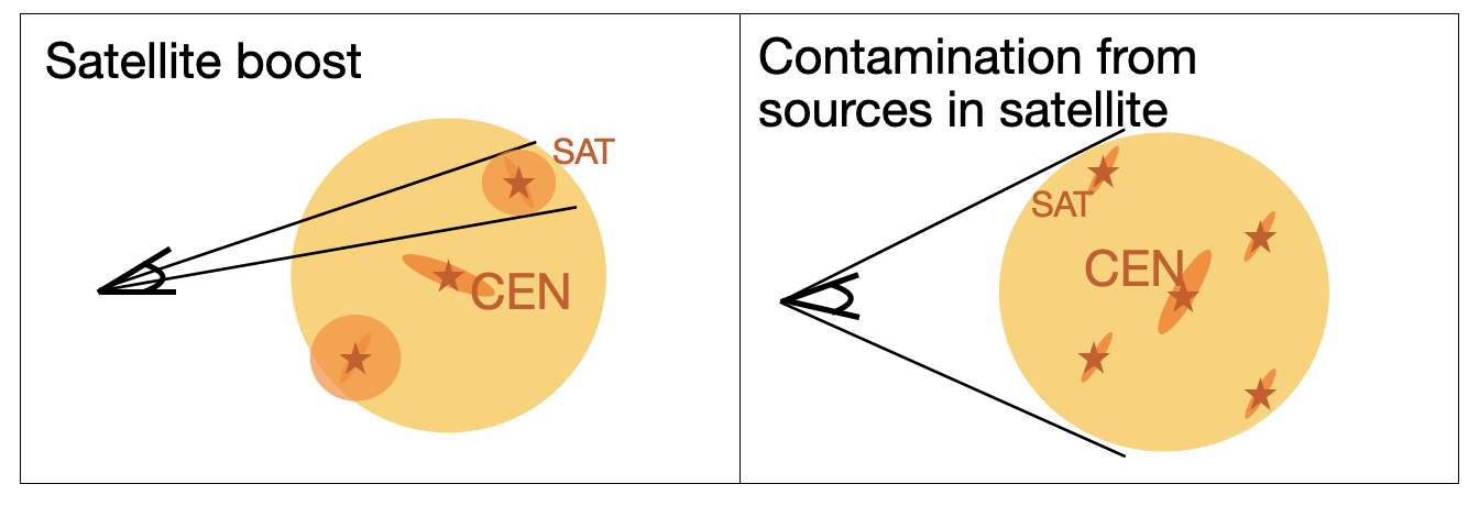
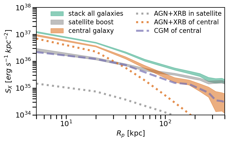
Figure 1: Top Panel: An illustration of contamination to the stacking from the satellite boost and sources in the satellites. Bottom Panel: An illustration of the X-ray surface brightness profiles of different components. The X-ray surface brightness profile of central galaxies that we are interested in (orange band) is obtained by subtracting the satellite boost (gray band) from the stacking of all galaxies (green band). The hot CGM X-ray emission of the central galaxy (purple dashed line) is modeled by subtracting the X-ray emission from the X-ray sources in satellite galaxies (gray dotted line) and central galaxies (orange dotted line) from the X-ray surface brightness profile of central galaxies (orange band).

Figure 2: An illustration of how the isolated selection works for photometric samples. If after projection, the virial halo of a galaxy has no overlap or is much more massive than overlapped galaxies, they are kept in the isolated galaxy sample (in orange color). Otherwise, they are removed (in color gray). The radius of the largest circle denotes the virial radius of the galaxy (not in scale).

3.6 Central galaxy selection from SDSS MGS

An unbiased selection of central galaxies requires accurate measurement of galaxy redshifts, the typical redshift uncertainty needs to be at least smaller than $10^{-4}$. For the SDSS MGS, it is possible to define a central galaxy sample, and different schemes exist to select central galaxies. A commonly used approach is the friends-of-friends (FoF) algorithm: galaxies are identified as a group according to the linking lengths, and within each group, the brightest galaxy is defined as the central galaxy (Crook et al., 2007; Robotham et al., 2011; Tempel et al., 2016). An alternative method is to define the locally brightest galaxies as central galaxies and other galaxies falling within a certain distance around them are satellites (Anderson et al., 2015; Comparat et al., 2022). More involved approaches include self-calibrated halo-based group finding (Yang et al., 2005; Tinker, 2022), group finder with galaxy weighting (Abdullah et al., 2018), Bayesian group finder based on marked point processes (Tempel et al., 2018).

Here, the self-calibrated halo-based group finding algorithm is applied to the SDSS MGS to classify the galaxy as central or satellite and estimate the halo mass (Tinker, 2021, 2022). The halo-based group finding algorithm searches for galaxy groups within the same dark matter halos and identifies the central galaxy. The algorithm is calibrated by the mock galaxy distributions and is further self-calibrated using the observations, including the galaxy clustering measurements, lensing, and satellite luminosity measurements. The algorithm assigns halos to self-calibrated galaxies by comparing the catalog to complementary data (Tinker, 2021). The algorithm’s performances are excellent: the halo masses of either star-forming or quiescent central galaxies agree well with the halo masses estimated from weak-lensing observation. The clustering properties, halo occupation distribution (HOD), and $M_{\rm h}-M_{*}$ relation of star-forming or quiescent galaxies are also well reproduced (Tinker, 2022).

For each galaxy in the SDSS MGS, its probability as central or satellite ($P_{\rm sat}$, we use the recommended $P_{\rm sat}=0.5$ as a boundary), and its host halo mass is provided in Tinker (2021).

Central galaxy sample in stellar mass bins (CEN)

The central galaxy sample (CEN) and satellite galaxy sample (SAT) selected from the SDSS MGS in stellar mass bins are listed in Table 8. In total, we have 85,222 central galaxies and 30,092 satellite galaxies.

Central galaxy sample in halo mass bins (CEN_halo)

With halo mass assigned to each galaxy in the SDSS MGS by the group finder algorithm, we can also study how the $M_{\rm halo}$ ($M_{\rm 200m}$) is related to the X-ray emission of galaxies. We define a halo mass-selected sample (we name it as CEN_halo sample) by splitting it into five logarithmic bins in the range $\log M_{\rm 200m}=11.5-14.0$ of 0.5 dex each, see Table 8. We set the maximum redshift for each sample at the redshift where these galaxy samples’ completeness is at 90% (for a magnitude cut $r_{AB}=17.77$). We have 125,512 central galaxies in the CEN_halo sample. The bins containing less than 1000 galaxies will not be stacked.

3.7 Isolated galaxy selection from LS DR9

Different from spectroscopic surveys such as SDSS, the central galaxy selection algorithm discussed above is not readily applicable to LS DR9 due to its photometric redshift uncertainties. Instead, we construct an ‘isolated’ galaxy sample from LS DR9 that is, as much as possible, free from satellite contamination.

We work with projected haloes, as we illustrate schematically in Fig. 2. For each galaxy, based on its stellar mass, we compute its mean virial radius ($R_{\rm vir}$) and the angle it subtends on the sky ($\theta_{\rm vir}$) using the stellar to halo mass relation from Moster et al. (2010). The virial radius definition is that of Bryan & Norman (1998). In the simplest case (case 1), if the virial halo of a galaxy has no overlap with other galaxy halos along the line of sight (i.e., the angular separation of a galaxy pair is larger than the sum of their virial radii), then we assume it is naturally central and does not suffer from satellite contamination. In the case where the virial halo of a galaxy overlaps with other galaxy halos along the line of the sight (case 2, case 3), we select the galaxy that is dominantly more massive (by a factor of two) and remove the smaller galaxy from the sample (case 2). If the two galaxies have comparable stellar masses (the stellar mass difference is smaller than two), we reject both galaxies. In this way, we get the central galaxy at least twice as massive as the most massive satellite galaxy in its halo. It means that the satellite boost and the contamination from the sources in satellite galaxies are reduced. On the other hand, the sample is a (incomplete) sub-sample of the central galaxy population living in under-dense environments. The X-ray background for the isolated galaxies is lower than the average X-ray background over the sky (due to the removal of foreground and background sources), and this is the necessity of taking $S_{\rm X,min}$ as the background (see the discussion in Appendix A). The selection of isolated galaxies has a low dependence on the photometric redshift accuracy of the galaxies. The selection method used to construct the isolated galaxy sample is validated through the mock galaxy catalog in Sect. 4.1.

Isolated galaxy sample (isolated)

Following the scheme defined above, we select the isolated galaxies from the FULL_phot sample to minimize the projected X-ray emission from nearby galaxies. Considering the dispersion of the $z_{\rm phot}$ and $M_{*}$ of LS DR9, we increase the ‘FULL_phot’ galaxy sample by retrieving galaxies with $z_{\rm phot}<z_{\rm max}+0.05$ and $M_{*}>1/2M_{\rm min}$ to avoid extra selection of isolated galaxy.

The fraction of isolated galaxies selected from the FULL_phot sample is 25% at the lower mass end, 17% for MW-mass bin, 8% for M31-mass bin, and 5% for 2M31-mass bin. Table 8 details the total number of isolated galaxies obtained for each sample. We name the isolated galaxy sample as ‘isolated’. In total, we have 213,514 isolated galaxies, about 2.5 times the CEN sample size, about 13 times larger than Comparat et al. (2022), 130 times larger than Chadayammuri et al. (2022) and close to the sample size of Anderson et al. (2015).

Two main differences exist between this isolated sample and the CEN sample. First, the isolated galaxies are central galaxies with at most $M_{\rm sat}=1/2M_{\rm cen}$ satellites in the halo, and the satellite boost is well removed. Therefore, the isolated galaxies are located in a less dense environment than the CEN sample and should be considered as a subsample of the central galaxy population. Second, the redshift distributions of the isolated and CEN samples are different, with the isolated sample extending to $z=0.4$. Therefore, when comparing the stacking results of the two samples, the redshift evolution needs to be considered. The PSF profiles of the two samples also differ on their physical scale.

4 Models

Given the complexity of the galaxy-halo relation, the possible contaminations from satellite galaxies, and unresolved X-ray sources (XRB and AGN), a robust interpretation of the stacking results requires reliable models to control all of the above effects. In this section, we introduce a mock galaxy catalog built from simulations to help control the properties of galaxy samples in Sect. 4.1. The X-ray emission from unresolved AGNs and XRBs in the stacked galaxies and satellite galaxies is modeled in Sect. 4.2. The contamination from the misclassified central galaxy in the group finder is modeled in Sect. 4.3

4.1 Mock galaxy catalog

We build a mock catalog to help characterize and gain insights into the designed galaxy samples. We use the Uchuu simulation (Ishiyama et al., 2021) and its UniverseMachine galaxy catalog (Behroozi et al., 2019). Uchuu simulation is a suite of ultra-large cosmological N-body simulations to construct the halo and sub-halo merger trees in a box of $2.0\rm h^{-1}Gpc$ side-length, with mass resolution of $3.27\times 10^{8}\rm h^{-1}M_{\odot}$, using the cosmological parameters obtained by Planck (Planck Collaboration et al., 2020; Ishiyama et al., 2021). The galaxy model well reproduces the stellar mass function and the separation between red-sequence and blue-cloud galaxies. We create a full-sky light cone following the method from Comparat et al. (2020).

We empirically calibrate the relation between stellar mass and K-band absolute magnitude (and its scatter) as a function of redshift using observations from SDSS, KIDS+VIKING, GAMA (for redshift smaller than 0.75) and COSMOS (for higher redshifts) (Ilbert et al., 2013; Almeida et al., 2023; Kuijken et al., 2019; Driver et al., 2022). With these relations, we assign an absolute K-band magnitude to each simulated galaxy using the stellar mass prediction from UniverseMachine. Then, we search the observed data sets for the nearest neighbor to each simulated galaxy in redshift and K-band. The set of observed broadband magnitudes (particularly the r-band) obtained with the match is assigned to the simulated galaxy. We find that the galaxy painting process is faithful to the observed galaxy population up to redshift $\sim$0.5. The mock catalog well reproduces the observed K-band and r-band luminosity functions from GAMA (or SDSS). We can thus apply the magnitude limit used in this work to the mock catalog. In the light cone, central and satellite galaxies are defined; we can thus test the reliability of the isolated selection scheme.

We build a mock LS DR9 catalog from the light cone to z=0.45. We apply the magnitude cut $r_{AB}<21$ to the light cone. We add a Gaussian distributed $z_{\rm error}$ and $M_{\rm error}$ with the same median and dispersion of the LS DR9 catalog to the corresponding accurate values provided by the light cone. Then we select the galaxies within the same $M_{*}$ and $z_{\rm phot}$ bins as FULL_phot to build the mock FULL_phot sample. We apply the isolated galaxy selection scheme to the mock FULL_phot sample and obtain a mock isolated sample. We use the mock samples to assess the isolated selection effect of our galaxy samples. In the mock FULL_phot sample, we find that the satellite fraction amounts to 25-35%. On the other hand, in the mock isolated sample, we get much lower satellite fractions, only 5-10%. In most cases, the satellite galaxies are kept since they are far away from other massive galaxies. A small portion of the satellite galaxies are misidentified due to the dispersion of $Z_{\rm phot}$ and $M_{*}$ of LS DR9. We also use the mock LS DR9 catalog to derive the stacked galaxies’ average underlying $M_{\rm halo}$ and $R_{\rm vir}$.

Similarly, we build a mock SDSS MGS catalog. We apply the magnitude cut $r_{AB}<17.77$ and add a Gaussian distributed $z_{\rm error}=10^{-4}$ and $M_{\rm error}=0.01\ \rm dex$ to the accurate ones from the light cone.

4.2 Models for AGN and XRB emission

The PSF and sensitivity of eROSITA prevent us from resolving all point sources at the redshift of the galaxies we stack. Therefore, to infer what fraction of the measured X-ray emission comes from the hot CGM, we need to build reliable AGN and XRB models and predict their emission. We opt for an empirical model to predict the XRB X-ray emission based on the stellar mass and SFR of galaxies (Sect. 4.2.1). For the AGN, we opt for an observation-based approach (Sect. 4.2.2 and Appendix. C). The X-ray emission of XRB in the satellite galaxies is modeled using the mock catalog (Sect. 4.2.3). With the predicted luminosity of the XRB and AGN, we normalize the PSF to obtain their X-ray surface brightness profiles.

4.2.1 Model for XRB

The X-ray luminosity of XRB in the 2-10 keV band ($L_{\rm 2-10keV}$) scales with SFR and $M_{*}$ of host galaxies (Lehmer et al., 2016; Aird et al., 2017). We predict the $L_{\rm 2-10keV}$ and estimate its uncertainty using the model in Aird et al. (2017) (see Equation.5 of Aird et al. (2017)). We convert $L_{\rm 2-10keV}$ to the X-ray luminosity in 0.5-2 keV ($L_{\rm XRB}$) by assuming an absorbed power law with a photon index of 1.8, and with column density fixed at $N_{H}=2.3\times 10^{20}\rm cm^{-2}$, the mean $N_{H}$ of the stacked area. We take the SFR of galaxies in SDSS MGS estimated by Brinchmann et al. (2004b) to predict the XRB emission of the CEN and CEN_halo samples. The average SFR of the isolated sample is estimated using the mock LS DR9 catalog.

4.2.2 Model for AGN

To modal the AGN emission for the CEN and CEN_halo samples, we consider galaxies identified as ‘AGN’ or ‘composite’ using the BPT diagram applied to the SDSS MGS central galaxies and name these galaxies as CENAGN sample (Baldwin et al., 1981; Brinchmann et al., 2004a). Depending on the stellar mass, $f_{\rm AGN}=$8-18% of the galaxies in the CEN sample are selected to CENAGN; see Table 6. We stack the galaxies in the CENAGN sample, masking all detected X-ray sources to calculate the maximum X-ray emission from unresolved AGN and XRB as described in Appendix. C. We estimate the AGN emission ($L_{\rm AGN}$) as the residual emission after subtracting the XRB emission. Under the assumption of no other galaxies hosting AGN, the lower limit of the average AGN contamination in the CEN sample is $L_{\rm AGN}\times f_{\rm AGN}$. To be conservative, we take the upper limit of AGN contamination as $2\times L_{\rm AGN}\times f_{\rm AGN}$; this accounts for (obscured) X-ray AGN not being identified as AGN or composite in the SDSS spectra. We repeat the procedure for the CEN_halo sample to estimate the AGN contamination there. We find that the unresolved AGN contamination is only about 25-50% of the XRB emission (see the discussion in Appendix. C).

There is no AGN catalog available for the isolated sample selected from the LS DR9 photometric survey. There are empirical AGN models derived from the AGN luminosity function and logN-logS (Aird et al., 2017; Comparat et al., 2019, 2023). However, the isolated galaxy selection criteria could introduce a selection effect to the AGN population. A proper AGN model for the isolated sample requires knowledge of the AGN halo occupation distribution and clustering properties to account for the sample selection properly, we leave the discussion for future work. In this paper, we use the CEN and CEN_halo samples to derive the X-ray emission from the CGM.

4.2.3 Unresolved point sources in satellite galaxies

The AGN and XRBs in the satellites would contaminate the hot CGM emission attributed to the central galaxy. We take the mock LS DR9 and SDSS MGS catalog to evaluate the satellite galaxy distribution. For each stacked galaxy, we select the galaxy with similar stellar mass (difference smaller than 0.1 dex) and redshift (difference smaller than 0.01) in the mock catalog. We count the number of satellite galaxies and the projected distances of the satellites to the mock central galaxy. The AGN population in satellite galaxies is unclear; there could be 0-20% satellite galaxies hosting AGN (Comparat et al., 2023). We assume the AGN contamination in the satellite galaxies is negligible after applying masks. We estimate the XRB emission of the satellites according to properties from the mock catalog, as in Sect. 4.2.1. we sum and average the XRB emission in satellites as a function of distance to the central galaxy.

We find the total X-ray luminosity of unresolved XRBs in satellites is about 8% (19%, 37%, 66%) of the XRB in the stacked central galaxies for the four $M_{*}$ bins in the CEN sample, respectively. Therefore, the model of unresolved point sources in satellites is necessary, especially for massive galaxies.

4.3 Model for misclassified central galaxies

The satellite galaxies might be misclassified as central in the group finder, with a chance of ¡1% (Tinker, 2021). In the case of stellar mass selection (CEN), since satellites are hosted by more massive (brighter in X-ray) haloes, the contamination can not be ignored. Here, we consider the 1% satellite galaxies in the CEN sample and model their contamination. We stack galaxies and measure the X-ray emission in the SAT sample ($S_{\rm X,SAT}$). We rescale the X-ray profiles of CEN ($(S_{\rm X,CEN}$) as $(S_{\rm X,CEN}-1\%S_{\rm X,SAT})/99\%$. The rescaled X-ray luminosity of CEN drops by about 5%.

5 X-ray surface brightness profile around galaxies from the FULL and SAT samples

In this section, we present the X-ray surface brightness profile of the FULL_phot sample, which is affected by the satellite boost effect (Sect. 5.1). We compare the X-ray surface brightness profiles of CEN and SAT samples to untangle the satellite boost effect from the stacking of the FULL_spec sample (Sect. 5.2).

5.1 X-ray surface brightness profile of FULL_phot sample

Figure 3: The X-ray surface brightness profiles of the FULL_phot sample after subtracting background, without masking sources. The results are divided into galaxy mass bins $\log(M_{*})=10.0-10.5$, 10.5-11.0 (MW-mass), and 11.0-11.025 (M31-mass) as labeled. The dotted line is the PSF of eROSITA, and the vertical dash-dotted line denotes the average virial radius of stacked galaxies. The X-ray emission comprises all effects mentioned in Sect. 3.5, limiting its interpretability regarding CGM emission. The X-ray surface brightness profile measured by stacking 16,142 galaxies with $\log(M_{*})=10.4-11.0$ and $z_{\rm spec}=0.05-0.3$ is plotted in gray (Comparat et al., 2022). The galaxy sample in Comparat et al. (2022) contains a complete population of AGN (while our FULL_phot does not contain sources that appear point-like in the legacy survey photometry) and has a broader PSF due to its higher mean redshift. So we expect the previous measurement to agree with the FULL MW-mass at large separation but to be brighter in the centre.

Stacking the FULL_spec or FULL_phot sample without masking any detected X-ray sources introduces the least uncertainty and bias (from X-ray data reduction or galaxy sample compiling) to the results; the measurement is reproducible. The surface brightness profiles of the FULL_phot samples in $\log(M_{*})=10.0-10.5$, MW-mass and M31-mass (after subtracting the background) are shown in Fig. 3.

We notice the significant improvement of the statistics by comparing the X-ray surface brightness profile to the one measured by stacking 16,142 galaxies with $\log(M_{*})=10.4-11.0$ and $z_{\rm spec}=0.05-0.3$ selected from the GAMA catalog using the eFEDS X-ray data (Comparat et al., 2022). The X-ray surface brightness profiles obtained have a high signal-to-noise ratio (S/N). For the MW-mass galaxies, the integrated luminosity measured within each 100 kpc has a S/N above 100. These high-significance measurements benefit from the large number of sources considered and the large area covered by X-ray observations.

Due to the satellite boost we described in Sect. 3.5, the satellite galaxies located in more massive dark matter halo strongly influence the profiles shown in Fig. 3, resulting in the stacked X-ray emission extending to about 1-2 Mpc (about 5-10 times of $R_{\rm vir}$ of galaxies). The X-ray sources contributing to these stacks include AGN, XRB, and hot gas emission: intra-cluster medium (ICM), intra-group medium (IGrM), and CGM from central and satellite galaxies in different massive halos. The interpretation of these measurements remains complex, and future simulation and modeling efforts will enable an unambiguous interpretation of all the signals present in these measurements. In Sect. 5.2, we briefly discuss the different X-ray surface brightness profiles around central and satellite galaxies. However, we leave the elaboration of an accurate satellite boost model that will enable the complete extraction of the information in these stacks with high signal-to-noise for future studies.

5.2 Untangle the X-ray emission from satellite and central galaxies in FULL_spec sample

Figure 4: The observed average X-ray surface brightness profile of galaxies in M31-mass bin of FULL_spec sample and the profiles after splitting FULL_spec sample to central (CEN) or satellite (SAT) galaxies. We scale the observed surface brightness profiles of CEN and SAT according to the number ratio of galaxies, namely, $f_{\rm SAT}=N_{\rm g,SAT}/N_{\rm g,FULL_{spec}}$ and $f_{\rm CEN}=N_{\rm g,CEN}/N_{\rm g,FULL_{spec}}$. The vertical dash-dotted line denotes the average virial radius of M31-mass galaxies in the FULL_spec sample.

The satellite boost biases the results of the stacking experiment. In this section, we use the central/satellite galaxy classification of the SDSS spectroscopic sample and stack the X-ray emission around galaxies in CEN and SAT samples to study the difference, and to untangle the X-ray surface brightness profile of central galaxies from the stacking of FULL_spec (or FULL_phot sample).

The comparison of the X-ray surface brightness profile of FULL_spec, CEN, and SAT sample is plotted in Fig. 4, taking the M31-mass bin as an example. As expected, galaxies with the same $M_{*}$ but classified as satellites or centrals have different X-ray surface brightness profiles. The satellite galaxy, residing in a more massive dark matter halo, has its X-ray emission boosted by the emission from virialized gas of the larger halo they reside in, from nearby centrals and other satellite galaxies. Consequently, the satellite galaxies’ X-ray surface brightness profile appears to be more extended and brighter than that of the central.

We rescale the profile of central or satellite galaxies by their number ratio. Namely, we multiply the average profile of central or satellite galaxies shown in the left panel by $N_{CEN}/N_{g}$ or $N_{SAT}/N_{g}$, respectively. These rescaled profiles of centrals and satellites, compared to the FULL_spec sample, are plotted in Fig. 4. We find that, beyond 100 kpc, the emission from satellite galaxies dominates over the central galaxy and determines the profile shape of the FULL_spec sample, as we had argued. This proves the necessity of selecting isolated or central galaxies to study how a galaxy modulates the properties of its CGM. On the other hand, we can use the rescaled profiles to untangle the emission in FULL_spec sample and model the influence of the misclassified central galaxy, as we discussed in Sect. 4.

We now focus on the isolated and CEN samples where the satellite boost that hampers the interpretation of the full stacks is minimized.

6 The circum-galactic medium of isolated and central galaxies selected in stellar mass

In this section, we mask all identified X-ray sources, so that the emission from the hot gas component becomes more discernible. The observed surface brightness profiles of the CEN and isolated samples are presented in Sect. 6.1. The X-ray emission from the hot CGM emission is modeled and presented in Sect. 6.2.

6.1 The X-ray surface brightness profiles

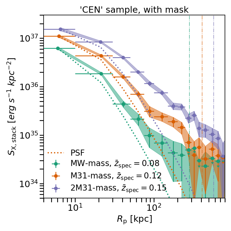
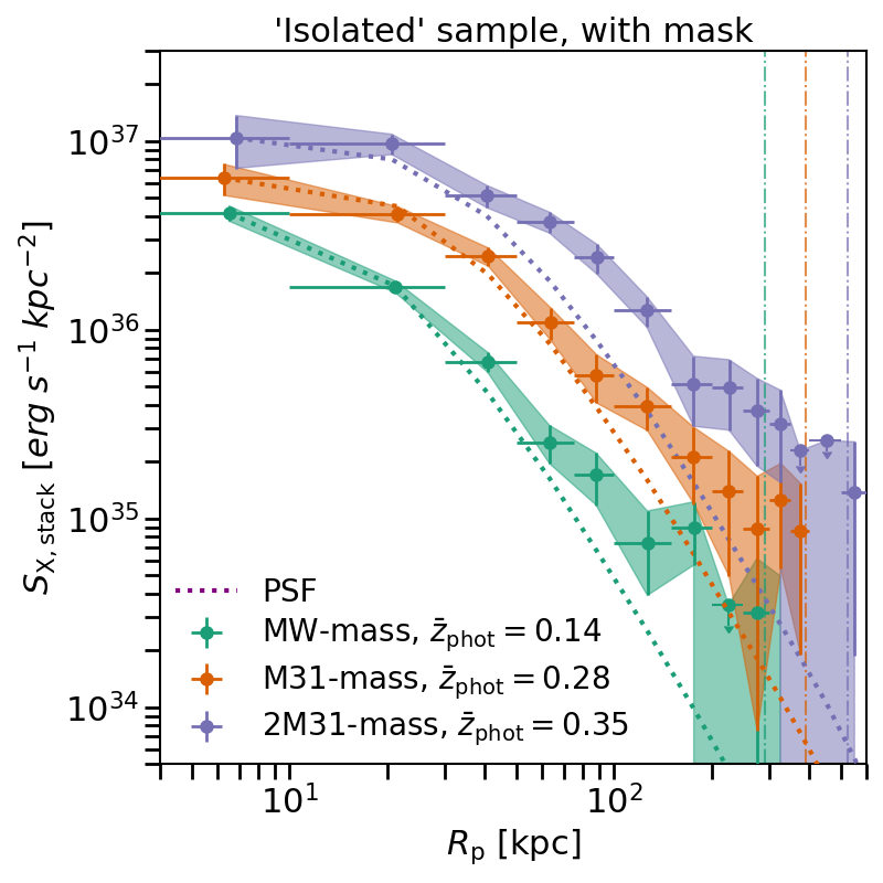
Figure 5: Left Panel: The average X-ray surface brightness profiles of central galaxies (with a magnitude limit of $r_{\rm AB}<17.77$) after subtracting background and masking X-ray sources, for galaxies with $\log(M_{*})=10.5-11.0$ (MW-mass), 11.0-11.25 (M31-mass) and 11.25-11.5 (2M31-mass). The X-ray emission comprises unresolved point sources and hot gas. $\bar{z}$ is the median redshift of galaxies in each mass bin. The dotted lines are the PSF of eROSITA. The vertical dash-dotted lines are the virial radius at different stellar mass bins correspondingly. Right Panel: Same as left but for the isolated sample (with a magnitude limit of $r_{\rm AB}<20$).

The X-ray surface brightness ($S_{\rm X,stack}$) profiles up to $R_{\rm vir}$ of the CEN (isolated) sample in MW-mass, M31-mass and 2M31-mass are plotted in the left (right) panel of Fig. 5. The X-ray emission detected here is the sum of unresolved point sources and hot gas emission from the stacked isolated or central galaxies (plus their satellite galaxies) within $R_{\rm vir}$.

We find that the X-ray surface brightness increases with stellar mass. The extended nature of the emission can be visually identified by comparing the X-ray surface brightness profile to the PSF of eROSITA (dotted line). Flatter profiles than the PSF are observed beyond 30 kpc for MW-mass and more massive galaxies (left panel of Fig. 5). The profile becomes more extended with increasing stellar mass. The X-ray emission is detected within the virial radius of galaxies with $S/N\approx 8.1,12.3,17.0$ for the MW-mass, M31-mass, and 2M31-mass galaxies in the CEN sample and $S/N\approx 8.8,6.4,7.2$ in the isolated sample. The X-ray emission is detected in $0.5-1R_{\rm vir}$ of galaxies with $S/N\approx 3.1,4.5,8.4$ for the MW-mass, M31-mass, and 2M31-mass galaxies in the CEN sample and $S/N\approx 2.3,2.3,2.0$ in the isolated sample.

We find that the emission starts to deviate significantly from the PSF at smaller radii in the CEN sample compared to the isolated sample. This results from the smaller average redshift of CEN sample, which implies higher spatial resolution. Therefore, the extended features of the detected X-ray profiles are more prominent. For the galaxies with the same mass, the observed profile of the isolated sample is flatter than the CEN sample. This is because the isolated galaxy sample has an average higher redshift and suffers more from the broader PSF on a physical scale, which we discuss more in Appendix D.

For the first time, we measure the extended X-ray emission up to the virial radius around the MW-mass and M31-mass isolated or central galaxies with a high signal-to-noise ratio.

6.2 The hot CGM emission in MW-mass or more massive galaxies

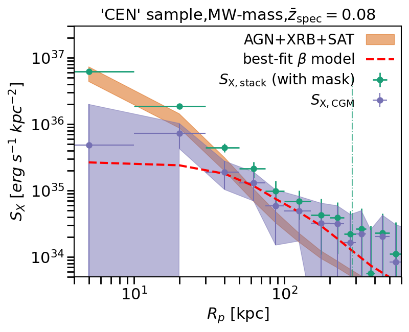
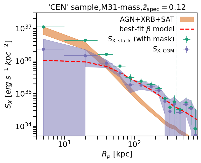
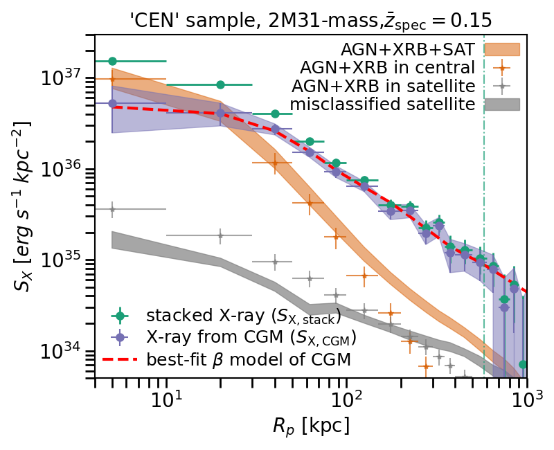
Figure 6: The average X-ray surface brightness profiles of central galaxies selected from SDSS in different $M_{*}$ bins, after masking X-ray sources (green points, $S_{\rm X,stack}$), the modeled X-ray emission from the unresolved AGN, XRB and misclassified centrals (orange band), and the emission from the CGM (purple band,$S_{\rm X,CGM}$) modeled by subtracting AGN and XRB from the $S_{\rm X,stack}$. The red dashed line is the best-fit of the CGM profile with a $\beta$ model. The vertical dash-dotted line is the virial radius, $R_{\rm vir}$. The top two panels are for MW-mass and M31-mass galaxies, and the bottom panel is for 2M31-mass galaxies. In the bottom panel, we further denote the X-ray surface brightness profiles of modeled unresolved AGN and XRB in the central galaxies (orange cross), in the satellite galaxies (gray cross), and X-ray surface brightness profile of misclassified satellite (gray band).

Table 4: The best-fit parameters of $\beta$ model for the X-ray surface brightness profiles of CGM for the CEN samples in three stellar mass bins.

	MW-mass	M31-mass	2M31-mass
$\beta$	$0.42_{-0.11}^{+0.12}$	$0.37_{-0.05}^{+0.10}$	$0.35_{-0.02}^{+0.02}$
$\log(S_{\rm X,0}[\rm erg/s/kpc^{2}])$	$35.5_{-0.5}^{+0.5}$	$36.1_{-0.3}^{+0.6}$	$36.8_{-0.2}^{+0.2}$
$r_{\rm c}[\rm kpc]$	$30_{-25}^{+40}$	$25_{-20}^{+40}$	$10_{-5}^{+10}$
$\chi^{2}$	3.1	4.7	4.5
d.o.f.	5	8	10
$\chi^{2}$/d.o.f.	0.61	0.59	0.45

In this section, we apply the models described in Sect. 4.2 and Sect. 4.3, including the unresolved AGN and XRB emission in the central and satellite galaxies, and the emission boost from the misclassified central galaxies, to the CEN sample to extract information on the intrinsic CGM profiles. We subtract the modeled emission from the X-ray surface brightness profile, and the residual X-ray emission is considered to be produced by the hot CGM ($S_{\rm X,CGM}$).

We only consider the CEN sample, where the S/N is higher, and the point source emission, especially the AGN, is easier to model than the isolated sample. The results for MW-mass, M31-mass, and 2M31-mass galaxies are presented in Fig. 6. The modeled X-ray emission from AGN, XRB, and misclassified central galaxies (plotted in orange) contributes to most of the emission within 20 kpc and is less extended than the detected X-ray emission (green dots). The X-ray emission from the hot CGM (purple band) is detected within $R_{\rm vir}$ with $S/N\approx 5.6,9.6,14.8$ for MW-mass, M31-mass and 2M31-mass galaxies; and within $R_{\rm 500c}$ with $S/N\approx 6.8,11.8,18.3$.

We fit the $\beta$ model (Eq. 3) to the hot CGM X-ray profile to obtain an analytical description of the results. The fit results are reported in Table 4. We get $\beta\approx 0.42$ for MW-mass galaxies and $\beta\approx 0.35$ for 2M31-mass galaxies. $\log(S_{\rm X,0})$ increases with $M_{*}$, while $r_{\rm c}$ is poorly constrained, limited by the uncertainty of modeled AGN, XRB, and misclassified central galaxies emission.

Beside the $\beta$ model, the exponential model is proposed to describe the inner hot CGM ‘corona’, $S_{\rm X,exp}=S_{\rm X,0}e^{-r/r_{\rm s}}$, where $r_{\rm s}$ is the scale radius with a value of some kiloparsecs (Yao et al., 2009; Locatelli et al., 2023). The X-ray profile of the exponential model after convolving with the PSF does not significantly deviate from the PSF. This is because, at the typical distance of our galaxy sample, the PSF of eROSITA (about tens kpc) is much larger than the typical value of $r_{\rm s}$ and smooths the sharp exponential profile, which makes it hard to separate from the point source emission. For MW-mass and M31-mass galaxies, adding an exponential model can improve the fit, while better point source models are needed for further investigation.

Before this work, the value of $\beta$ had been measured in several nearby massive galaxies ($\log(M_{*})\approx 11.5$), within $0.5R_{\rm vir}$ with $\beta\approx 0.397\pm 0.009$, which is consistent with our measurement (Li et al., 2017, 2018). The hot CGM density profile beyond $0.5R_{\rm vir}$ is not well studied yet, as a result, the baryon budget stored in the hot CGM is poorly constrained by the X-ray observations (Li et al., 2018; Das et al., 2020, 2023). With our newly measured hot CGM density profile within $R_{\rm vir}$ for MW-mass galaxies, we estimate the baryon mass and fraction in Sect. 8.

7 X-ray emission of central galaxies in $M_{\rm halo}$ bins

Figure 7: The average X-ray surface brightness profiles of central galaxies with $\log(M_{\rm 200m})=12.0-13.5$ after subtracting background, and masking X-ray point sources. The dotted lines are the PSF of eROSITA. The vertical dashed lines are the virial radius at different halo mass bins correspondingly.

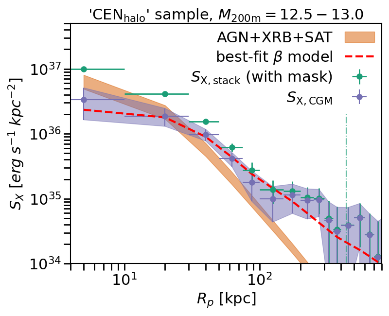
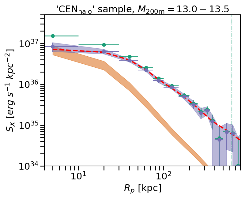
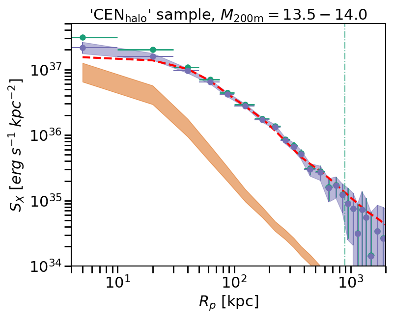
Figure 8: The average X-ray surface brightness profiles of CEN_halo sample in three different halo mass bins, after masking X-ray point sources (green points), the X-ray emission from the unresolved AGN, XRB (orange band) and the X-ray emission from the hot CGM (purple band), constructed by subtracting the AGN model to the total stack. The red dashed line is the best-fit of the hot CGM profile with a $\beta$ model. The vertical dash-dotted line is the $R_{\rm vir}$. From top to bottom: $M_{\rm 200m}=12.5-13.0$, 13.0-13.5, 13.5-14.0.

Table 5: The best-fit parameters of $\beta$ model for the X-ray surface brightness profiles of hot gas in CEN_halo sample.

		$\log(M_{\rm 200m})$
	12.5-13.0	13.0-13.5	13.5-14.0
$\beta$	$0.38_{-0.04}^{+0.07}$	$0.40_{-0.02}^{+0.03}$	$0.40_{-0.01}^{+0.01}$
$\log(S_{\rm X,0}[\rm erg/s/kpc^{2}])$	$36.7_{-0.3}^{+0.8}$	$37.0_{-0.1}^{+0.1}$	$37.3_{-0.1}^{+0.1}$
$r_{\rm c}[\rm kpc]$	$6_{-5}^{+10}$	$14_{-4}^{+5}$	$22_{-4}^{+5}$
$\chi^{2}$	4.4	4.3	10.0
d.o.f.	9	11	13
$\chi^{2}$/d.o.f.	0.49	0.39	0.77

We stack the CEN_halo sample to study how the X-ray emission relates to the halo mass. The X-ray surface brightness profiles of galaxies with $\log(M_{\rm 200m})=12.0-13.5$ after masking X-ray point sources are plotted in Fig. 7. We find that the X-ray surface brightness increases with $M_{\rm 200m}$. Extended emission is detected around central galaxies in halos with $\log(M_{\rm 200m})>12.5$. The X-ray emission comprises the hot gas and unresolved point sources within the halo. We model the unresolved point sources to obtain the residual X-ray surface brightness profiles of hot CGM (see Fig. 8). We fit the profiles of hot gas with the $\beta$ model, and the results are listed in Table 5. We get $\beta\approx 0.4$.

8 The baryon budget

Figure 9: The measured baryon fraction ($f_{\rm b}$) as a function of $M_{*}$, the baryon fraction is the sum of the stellar and the hot CGM within $R_{\rm vir}$ divided by the virial mass ($f_{\rm b}=(M_{\rm hot\,CGM}+M_{*})/M_{\rm vir}$). We assume the metallicity abundance of the hot CGM is $0.1Z_{\odot}$ (orange), $0.3Z_{\odot}$ (purple) and $Z_{\odot}$ (green), and the temperature of the hot CGM is at virial temperature ($T_{\rm vir}$) or half ($0.5T_{\rm vir}$). The dashed line ($f_{\rm b}=0.17$) is the predicted baryon fraction. The gray points are taken from tSZ measurements (Das et al., 2023), and X-ray emission measurements (Li et al., 2018; Das et al., 2020).

Based on the derived parameters of $\beta$ models in Sect. 6.2, we estimate the baryon mass and baryon fraction within $R_{\rm vir}$ of central galaxies. The density profile of the hot CGM in the $\beta$ model is

$$n(r)=n_{0}\left[1+\left(\frac{r}{r_{\rm c}}\right)^{2}\right]^{(-\frac{3}{2}\beta)}\ [\rm cm^{-3}],$$ (4)

where $n_{0}$ is the gas density at the galaxy center and is expressed as

$$n_{0}=\sqrt{\frac{10^{14}S_{X,0}\Gamma(3\beta)}{\sqrt{\pi}\epsilon_{\rm X}\frac{n_{\rm e}}{n_{\rm H}}r_{\rm c}\Gamma(3\beta-1/2)}}[\rm cm^{-3}],$$ (5)

where $n_{\rm e}$ and $n_{\rm H}$ are the number densities of electrons and hydrogens (Ge et al., 2016). We take the APEC model to estimate $\epsilon_{\rm X}(T,Z)$, which is the normalized X-ray flux of thermal plasma with temperature $T$ and metal abundance $Z$ (Smith et al., 2001). We assume the temperature of the hot CGM is at the virial temperature $T_{\rm vir}$, which can be derived from the $M_{\rm vir}$ and $R_{\rm vir}$ . The X-ray emissivity of the hot CGM at the $T_{\rm vir}<1\rm keV$ depends strongly on the metallicity abundance, which is not well studied for the MW-mass galaxies yet. We take values of $0.1Z_{\odot}$, $0.3Z_{\odot}$ and $Z_{\odot}$ to estimate $\epsilon_{\rm X}(T,Z)$. $Z_{\odot}$ is detected at massive galaxy groups, and we take it as an upper limit (Gastaldello et al., 2021), $0.1Z_{\odot}$ is reported from the CGM of the Milky-Way (Ponti et al., 2023), and $0.3Z_{\odot}$ is a commonly used value for the hot CGM.

The hot CGM mass ($M_{\rm CGM}$) is calculated by integrating the density profile of the hot CGM within $R_{\rm vir}$. We sum the hot CGM and stellar mass $M_{\rm b}=M_{\rm CGM}+M_{*}$, and calculate the baryon fraction by $f_{\rm b}=M_{\rm b}/M_{\rm vir}$. The result of central galaxies with $\log(M_{*})=10.5-11.5$ are presented in Fig. 9. The uncertainty is estimated by propagating the 1$\sigma$ uncertainty of $\beta$ model.

The $\Lambda CDM$ cosmology theory predicts $f_{\rm b}\approx 17\%$, as the dash line in Fig. 9. Our measured $f_{\rm b}$ is below the $\Lambda CDM$ cosmology theory predicted. We compare our measurements to the $f_{\rm b}$ measured based on the X-ray emission and tSZ and find consistent results within $1\sigma$ (Li et al., 2018; Das et al., 2020, 2023). There are several possible reasons for the low $f_{\rm b}$. First, we did not consider the other phases of the CGM, namely, the less hot components that are not measured by the X-ray emission. Secondly, the hot CGM around the galaxies may not be virialized and does not reach hydrostatic equilibrium; our assumption of the virial temperature is wrong. We calculate $f_{\rm b}$ by assuming $1/2T_{\rm vir}$ and find $f_{\rm b}$ increases by 0-5%.

Indeed, measuring the baryon mass through the X-ray emission method relies on the accurate assumption of the properties of the hot CGM. Our result only constitutes a first approximation and does not reflect the wealth of physical processes at stakes in the CGM (Faucher-Giguere & Oh, 2023). We leave the detailed inference of the different baryonic components and their properties for future studies. With the progress of the metallicity abundance and temperature measurement, point source models, and better statistics from larger galaxy samples in the future, we can set better constraints on the CGM density profile of MW-mass and M31-mass galaxies. In particular, the X-ray microcalorimeter observations, with a high energy resolution, are expected to contribute significantly to this endeavor (Nandra et al., 2013; XRISM Science Team, 2020; Cui et al., 2020).

9 Summary and conclusions

In this article, we provide the new detection of the X-ray emission from the hot circum-galactic medium around large, statistical samples of (massive) galaxies. We use the eRASS:4 X-ray data over an extra-galactic sky of about 11,000 square degrees. We achieved a significant step forward in understanding the influence and possible bias from the satellite galaxies (Fig. 1, Fig. 3 and Fig. 4). With the SDSS (spectroscopic) galaxy catalog and the group finder algorithm applied, we built two galaxy samples containing about 85,222 central galaxies split into stellar mass bins and 125,512 central galaxies split in halo mass bins (Table 8). In addition, we defined an isolated galaxy selection criteria that selects a sub-sample of central galaxies located in a sparse environment (Fig. 2). We built a galaxy sample from the LS DR9 (photometric) galaxy catalog, containing 213,514 isolated galaxies. Based on the observation, we built an AGN model (Appendix. C), and carefully modeled the components that can contaminate the CGM emission.

We stacked the galaxies, and the statistics we gained support the following main findings:

1. The X-ray surface brightness profiles are measured for $\log(M_{*})>10.0$ or $\log(M_{\rm 200m})>11.5$ central galaxies, and $\log(M_{*})>9.5$ isolated galaxies. (Fig. 5 and Fig. 7 ). We detect the extended X-ray emission around MW-mass and more massive galaxy population out to $R_{\rm vir}$. The signal-to-noise ratio of the extended emission around M31-mass (MW-mass) central galaxy is $12.3\sigma$ ($8.1\sigma$) within $R_{\rm vir}$, and is $4.5\sigma$ ($3.1\sigma$) within $(0.5-1)R_{\rm vir}$.

2. Using the models, we obtain the X-ray surface brightness profile of hot CGM for central MW-mass and more massive galaxies out to $R_{\rm vir}$ (Fig. 6). Using a $\beta$ model to describe the profiles, we get $\beta\approx 0.35-0.4$ for MW-mass and more massive galaxies (Table 4).

3. The X-ray surface brightness profiles of the hot CGM for central galaxies located in halo with $\log(M_{\rm 200m})>12.5$ are measured.(Fig. 8). We get $\beta\approx 0.4$ (Table 5).

4. With standard assumptions on the metallicity and temperature of the hot CGM, the baryon fraction of MW-mass and more massive galaxies is estimated to be lower than the $\Lambda CDM$ cosmology theory predicted (Fig. 9).

The eROSITA sky survey yields a vast repository of X-ray data across the sky, with abundant information on the hot CGM that invites further investigation and analysis. The measured X-ray surface brightness profiles of the FULL_phot have a high signal-to-noise ratio, which allows for building a complete model including the galaxy distribution and X-ray properties of the galaxy (Shreeram et al. in preparation). With deeper galaxy surveys, i.e., 4MOST, DESI, we can enlarge the galaxy sample, increase the statistics, and obtain a better view of the hot CGM around dwarf galaxies ($\log(M_{*})<10$).

With the progress of the X-ray microcalorimeter observations, we will obtain a better knowledge of the metallicity and temperature of the CGM, to derive its density profile.

Appendix A Validation of background calculation

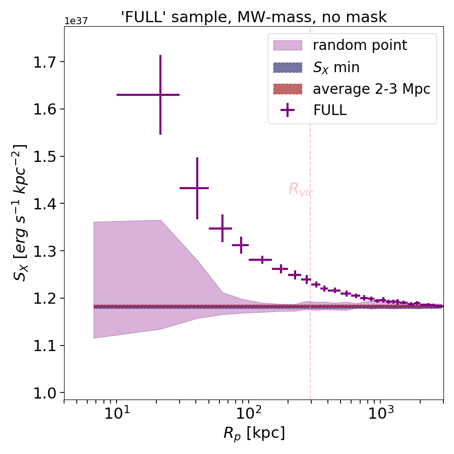
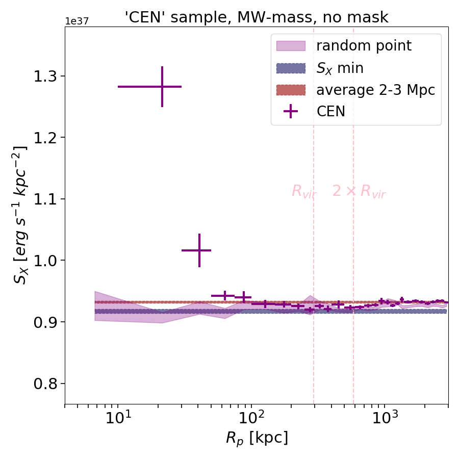
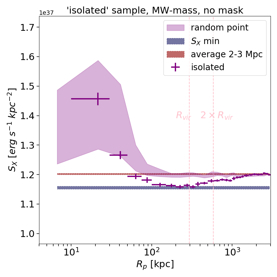
Figure 10: The observed X-ray surface brightness profiles of FULL_phot sample (left), CEN sample (middle) and isolated sample (right), without masking X-ray sources. The data points are the observed X-ray surface brightness profile, the colored bands are the estimated background by taking the random points (purple), the minimum X-ray surface brightness (blue) and the average X-ray surface brightness within 2-3 Mpc (red).

We test different methods to estimate the average background for the stacked galaxies.

a) We retrieve events within 3 Mpc of a random point near each galaxy ($\rm CUBE_{rd}$). The random point is within $1-4\times R_{\rm vir}$ of the galaxy. We merge $\rm CUBE_{rd}$ of each galaxy sample and calculate the average $S_{\rm X,rd}$ within 3 Mpc. As $\rm CUBE_{rd}$ randomly distributes over the sky area of stacked galaxies, $S_{\rm X,rd}$ is the average X-ray background of the stacked area.

b) We estimate the background surface brightness ($S_{\rm X,Mpc}$) by taking the average $S_{\rm X,gal}$ within the annulus at 2-3 Mpc distance from the center. The annulus choice of the $S_{\rm X,Mpc}$ guarantees that it is well beyond the virial radius of the largest haloes, i.e., galaxy clusters.

c) We define $S_{\rm X,min}$ as the minimum value of $S_{\rm X,gal}$ between $R_{\rm 500c}$ and $2\times R_{\rm vir}$.

The X-ray surface brightness profiles of MW-mass galaxies in the FULL_phot, isolated and CEN samples compared to different backgrounds are presented in Fig. 10. Beyond about 2 Mpc, the X-ray surface brightness profiles converge to $S_{\rm X,rd}$, the average X-ray background of the stacked area. The uncertainty of the background from jackknife re-sampling is about 0.2%. For the FULL_phot sample, the difference between the three backgrounds is less than 0.3%. We take the background of FULL_phot sample as $S_{\rm X,Mpc}$. The X-ray surface brightness of the CEN sample in the MW-mass bin has a stronger fluctuation with radius. The X-ray profile decreases until $1-2\ R_{\rm vir}$, then increases to the $S_{\rm X,rd}$ (agrees within 1$\sigma$). The difference between the three backgrounds is about $1.5\%S_{\rm X,rd}$. For the isolated sample, the X-ray surface brightness increases significantly beyond $R_{\rm vir}$ until agreeing with the $S_{\rm X,rd}$. This is because, by construction, the isolated sample contains galaxies located in a sparse environment where the local X-ray background is lower (see Section 3.7). We take $S_{\rm X,min}$ as the proper local background of the central and isolated galaxy sample.

The background surface brightness is redshift-dependent in units of $\rm erg/s/kpc^{2}$. The $S_{\rm X,rd}$ background levels of the isolated and CEN samples are therefore different by a factor of about $(\frac{1+z_{\rm iso}}{1+z_{\rm cen}})^{5}$, where $z_{\rm iso}$ and $z_{\rm cen}$ are the median redshifts of the isolated and ‘CEN’ sample.

Appendix B Merge SGA catalog to LS DR9 catalog

The SGA is a multi-wavelength atlas of nearby galaxies selected from DESI Legacy Imaging Surveys DR9. The selection is based on the apparent angular diameter of galaxies that are large enough to be spatially resolved. In the western Galactic hemisphere, there are 194527 galaxies in the SGA catalog. We match SGA to the LS DR9 catalog and find about 15% galaxies in SGA have no match in LS DR9. We add the missing SGA galaxies to the LS DR9 catalog to avoid losing the nearby massive galaxies.

No $M_{*}$ information is provided in SGA, and about 34% of SGA galaxies have no redshift estimation. For SGA galaxies with a redshift estimate, we estimate the stellar mass by the SED fitting using the three optical bands (g,r,z) and two infrared bands (W1, W2), following the method in Zou et al. (2019). The galaxies without redshift estimation are thrown away due to the difficulty of estimating stellar mass. There are about 5% galaxies that fall in the stacking area with no photometry information and low-quality redshift and $M_{*}$, which we throw away. We match the remaining SGA galaxies to GAMA and find that our derived redshift and $M_{*}$ are good quality. We add the 15,735 missing SGA galaxies with $\log(M_{*})>9$ to the LS DR9 catalog. 90% of these galaxies have $z<0.1$.

Besides, galaxies in the LS DR9 catalog could be too close to the bright nearby SGA galaxy. This may affect the accuracy of $z_{\rm phot}$ or $M_{*}$ in the LS DR9 catalog. We mask the LS DR9 galaxies that are within the $R_{25}$ of SGA galaxies, where $R_{25}$ is the approximate major-axis radius at the $25\,\rm mag\ arcsec^{-2}$, which can be taken as the radius of galaxy disk. Notice that we did not consider the inclination and position angle of the SGA galaxy. The procedure above removes $0.01\%$ of LS DR9 galaxies.

Appendix C AGN model for CEN sample

Table 6: The percentage and number of galaxy hosting AGN in CEN sample, identified using the BPT diagram (Baldwin et al. 1981; Brinchmann et al. 2004a).

$\log(M_{*})$	$f_{\rm AGN}$	$N_{\rm CENAGN}$
10.0-10.5	16%	1261
10.5-11.0	18%	5421
11.0-11.25	14%	3447
11.25-11.5	8%	1505

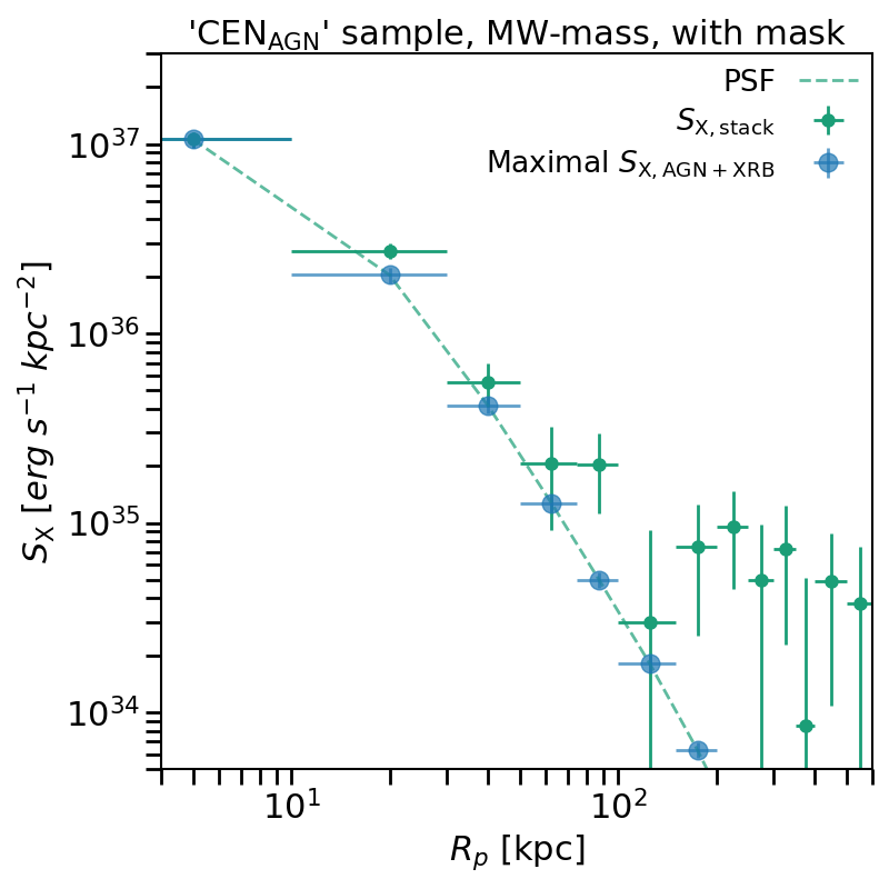
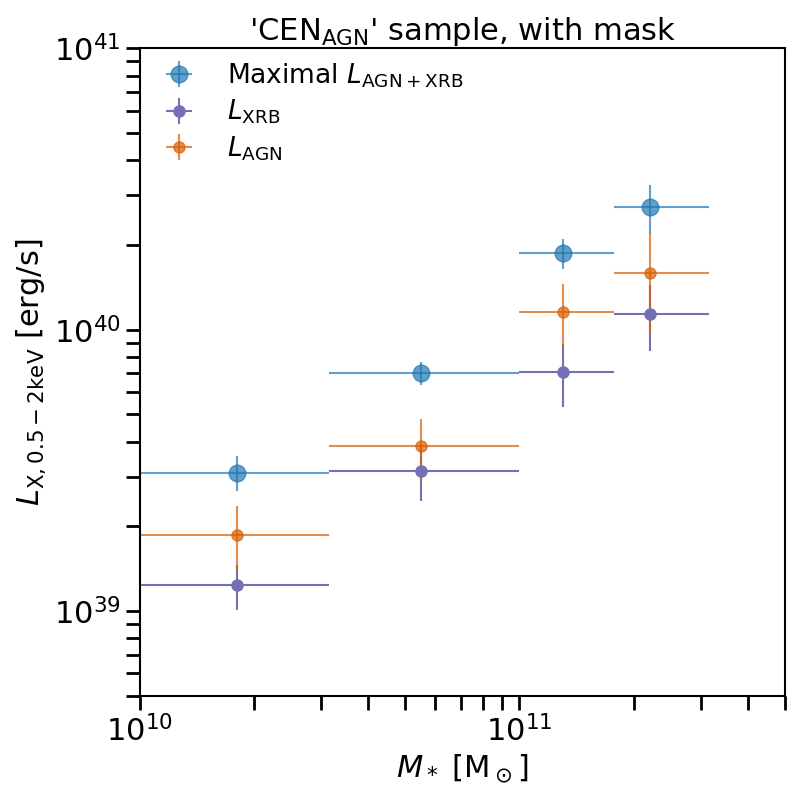
Figure 11: Left: The X-ray surface brightness profile of MW-mass galaxies in CEN_AGN sample, after subtracting background and masking X-ray sources (green points), the maximal X-ray emission from the unresolved point sources (blue points), in the shape of PSF (green dashed line). Right: The observed maximal X-ray luminosity of unresolved point source (blue), the model predicted XRB luminosity (purple), and the residual X-ray luminosity of unresolved AGN.

We estimate the AGN contamination in the CEN sample based on observations. We select the central galaxies hosting AGN, identified as AGN or composite, based on the BPT diagram, and name it as CEN_AGN (Baldwin et al. 1981; Brinchmann et al. 2004a). The percentage of central galaxies identified as hosting AGN ($f_{\rm AGN}$) is listed in Table 6. We stack the CEN_AGN sample in the same bins as the CEN sample, and mask detected X-ray sources. The obtained X-ray surface brightness profile for the MW-mass CEN_AGN galaxies is plotted in the left panel of Fig. 11. The maximal X-ray emission originating from the unresolved point sources (AGN and XRB) in the stacked galaxies should be in the shape of PSF, with the first bin as bright as detected (green dots). The maximal X-ray luminosity of the unresolved point sources is calculated by integrating the X-ray emission in the shape of PSF out to $R_{\rm 500c}$. We subtract the XRB luminosity predicted by the empirical model ($L_{\rm XRB}$) (Aird et al. 2017), and obtain the maximal unresolved AGN emission in the stacked galaxies ($L_{\rm AGN}$), see right panel of Fig. 11. The unresolved AGN in the CEN_AGN sample is slightly brighter than the XRB, less than two times. Notice that the stacked galaxies are identified as hosting AGNs and only account for $<20\%$ of the CEN sample; we summarise that the unresolved AGN emission is subdominant compared to the XRBs, and the uncertainty of the AGN model does not affect our results significantly.

Appendix D Compare the X-ray surface brightness profiles of isolated and CEN samples

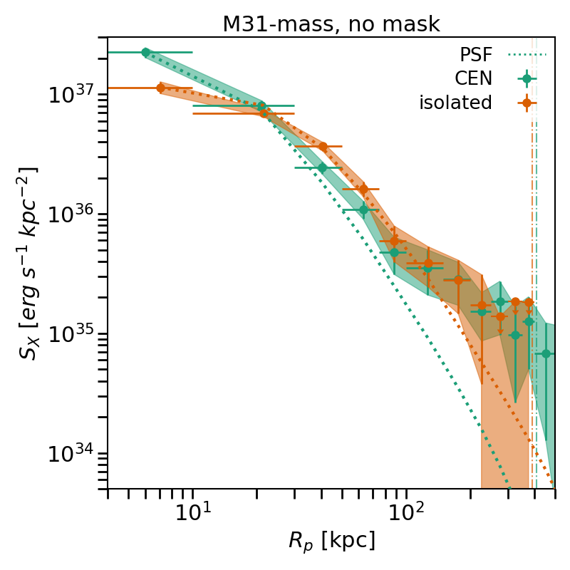
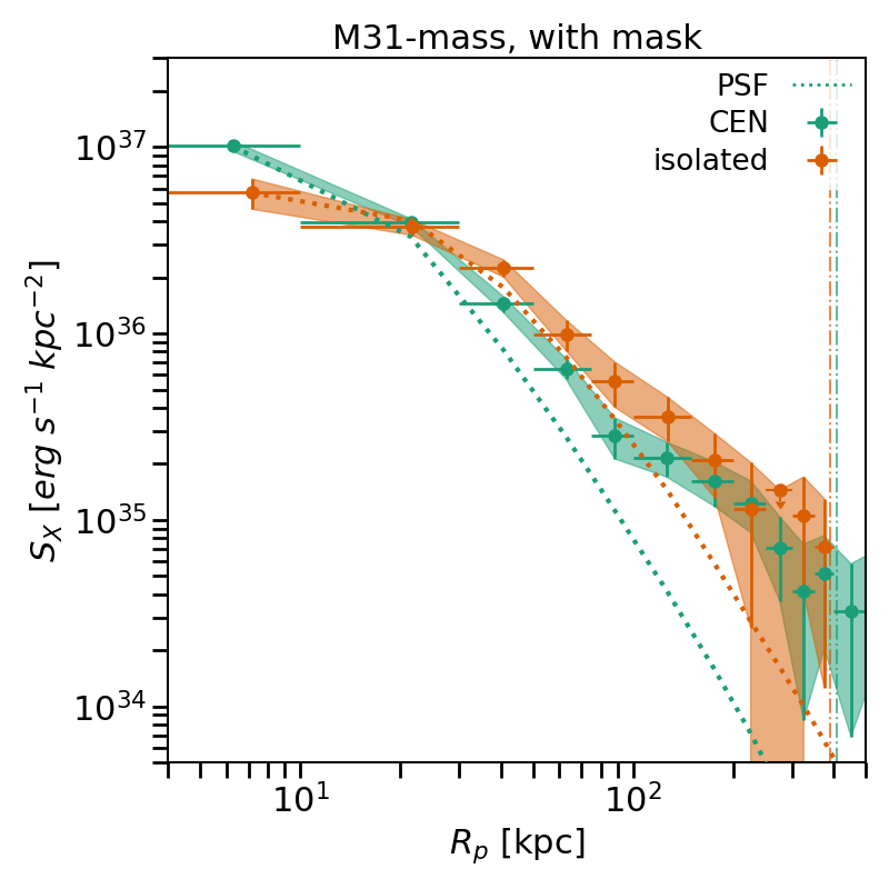
Figure 12: The X-ray surface brightness profiles of M31-mass galaxies from isolated and CEN samples after subtracting background, without (left) and with (right) masking X-ray sources. The dotted lines are the PSF of eROSITA. The vertical dash-dotted lines are the average virial radius of M31-mass galaxies.

The comparison of the X-ray surface brightness profiles of isolated and CEN samples, taking the M31-mass bin as an example, is shown in Fig. 12. The X-ray surface brightness profile of the CEN sample is sharper than isolated galaxies within 100 kpc. This is due to the lower average redshift of the CEN sample, which makes the PSF smaller on the physical scale. Beyond about 100 kpc, where the PSF influence is low, the X-ray emission of CEN and isolated galaxies is comparable.

Due to the selection criteria of the isolated sample, we expect the isolated galaxies to be located in a more sparse environment than the central galaxies, presenting a fainter or steeper X-ray surface brightness profile at a large scale. However, we did not detect this feature, limited by the statistics.

The other influence of the different redshift distributions of isolated and CEN samples is the masking of X-ray sources. Fewer X-ray sources are detected because the isolated sample has a higher average redshift. The X-ray surface brightness profile of the isolated sample after masking X-ray sources is slightly higher than the CEN sample (see the right panel of Fig. 12).

References

- Abazajian et al. (2009) Abazajian, K. N., Adelman-McCarthy, J. K., Agüeros, M. A., et al. 2009, ApJS, 182, 543
- Abbott et al. (2018) Abbott, T. M. C., Abdalla, F. B., Allam, S., et al. 2018, ApJS, 239, 18
- Abdullah et al. (2018) Abdullah, M. H., Wilson, G., & Klypin, A. 2018, ApJ, 861, 22
- Aihara et al. (2018) Aihara, H., Armstrong, R., Bickerton, S., et al. 2018, PASJ, 70, S8
- Aiola et al. (2020) Aiola, S., Calabrese, E., Maurin, L., et al. 2020, J. Cosmology Astropart. Phys., 2020, 047
- Aird et al. (2017) Aird, J., Coil, A. L., & Georgakakis, A. 2017, MNRAS, 465, 3390
- Almeida et al. (2023) Almeida, A., Anderson, S. F., Argudo-Fernández, M., et al. 2023, arXiv e-prints, arXiv:2301.07688
- Anderson et al. (2016) Anderson, M. E., Churazov, E., & Bregman, J. N. 2016, MNRAS, 455, 227
- Anderson et al. (2015) Anderson, M. E., Gaspari, M., White, S. D. M., Wang, W., & Dai, X. 2015, MNRAS, 449, 3806
- Andrae (2010) Andrae, R. 2010, arXiv e-prints, arXiv:1009.2755
- Arnouts et al. (1999) Arnouts, S., Cristiani, S., Moscardini, L., et al. 1999, MNRAS, 310, 540
- Baldwin et al. (1981) Baldwin, J. A., Phillips, M. M., & Terlevich, R. 1981, PASP, 93, 5
- Beckwith et al. (2006) Beckwith, S. V. W., Stiavelli, M., Koekemoer, A. M., et al. 2006, AJ, 132, 1729
- Behroozi et al. (2019) Behroozi, P., Wechsler, R. H., Hearin, A. P., & Conroy, C. 2019, MNRAS, 488, 3143
- Bilicki et al. (2021) Bilicki, M., Dvornik, A., Hoekstra, H., et al. 2021, A&A, 653, A82
- Bilicki et al. (2014) Bilicki, M., Jarrett, T. H., Peacock, J. A., Cluver, M. E., & Steward, L. 2014, ApJS, 210, 9
- Bilicki et al. (2016) Bilicki, M., Peacock, J. A., Jarrett, T. H., et al. 2016, ApJS, 225, 5
- Blanton et al. (2005) Blanton, M. R., Schlegel, D. J., Strauss, M. A., et al. 2005, AJ, 129, 2562
- Bogdán et al. (2013) Bogdán, Á., Forman, W. R., Vogelsberger, M., et al. 2013, ApJ, 772, 97
- Bogdán et al. (2015) Bogdán, Á., Vogelsberger, M., Kraft, R. P., et al. 2015, ApJ, 804, 72
- Brinchmann et al. (2004a) Brinchmann, J., Charlot, S., White, S. D. M., et al. 2004a, MNRAS, 351, 1151
- Brinchmann et al. (2004b) Brinchmann, J., Charlot, S., White, S. D. M., et al. 2004b, MNRAS, 351, 1151
- Brunner et al. (2022) Brunner, H., Liu, T., Lamer, G., et al. 2022, A&A, 661, A1
- Bruzual & Charlot (2003) Bruzual, G. & Charlot, S. 2003, MNRAS, 344, 1000
- Bryan & Norman (1998) Bryan, G. L. & Norman, M. L. 1998, ApJ, 495, 80
- Cavaliere & Fusco-Femiano (1976) Cavaliere, A. & Fusco-Femiano, R. 1976, A&A, 49, 137
- Chadayammuri et al. (2022) Chadayammuri, U., Bogdán, Á., Oppenheimer, B. D., et al. 2022, ApJ, 936, L15
- Comparat et al. (2023) Comparat, J., Luo, W., Merloni, A., et al. 2023, arXiv e-prints, arXiv:2301.01388
- Comparat et al. (2020) Comparat, J., Merloni, A., Dwelly, T., et al. 2020, A&A, 636, A97
- Comparat et al. (2019) Comparat, J., Merloni, A., Salvato, M., et al. 2019, MNRAS, 487, 2005
- Comparat et al. (2022) Comparat, J., Truong, N., Merloni, A., et al. 2022, A&A, 666, A156
- Coupon et al. (2015) Coupon, J., Arnouts, S., van Waerbeke, L., et al. 2015, MNRAS, 449, 1352
- Crook et al. (2007) Crook, A. C., Huchra, J. P., Martimbeau, N., et al. 2007, ApJ, 655, 790
- Cui et al. (2020) Cui, W., Chen, L. B., Gao, B., et al. 2020, Journal of Low Temperature Physics, 199, 502
- Dai et al. (2012) Dai, X., Anderson, M. E., Bregman, J. N., & Miller, J. M. 2012, ApJ, 755, 107
- Das et al. (2023) Das, S., Chiang, Y.-K., & Mathur, S. 2023, ApJ, 951, 125
- Das et al. (2020) Das, S., Mathur, S., & Gupta, A. 2020, ApJ, 897, 63
- de Jong et al. (2019) de Jong, R. S., Agertz, O., Berbel, A. A., et al. 2019, The Messenger, 175, 3
- DESI Collaboration et al. (2016) DESI Collaboration, Aghamousa, A., Aguilar, J., et al. 2016, arXiv e-prints, arXiv:1611.00036
- Dey et al. (2019) Dey, A., Schlegel, D. J., Lang, D., et al. 2019, AJ, 157, 168
- Driver et al. (2022) Driver, S. P., Bellstedt, S., Robotham, A. S. G., et al. 2022, MNRAS, 513, 439
- Faucher-Giguere & Oh (2023) Faucher-Giguere, C.-A. & Oh, S. P. 2023, arXiv e-prints, arXiv:2301.10253
- Finoguenov et al. (2019) Finoguenov, A., Merloni, A., Comparat, J., et al. 2019, The Messenger, 175, 39
- Gastaldello et al. (2021) Gastaldello, F., Simionescu, A., Mernier, F., et al. 2021, Universe, 7, 208
- Ge et al. (2016) Ge, C., Wang, Q. D., Tripp, T. M., et al. 2016, MNRAS, 459, 366
- HI4PI Collaboration et al. (2016) HI4PI Collaboration, Ben Bekhti, N., Flöer, L., et al. 2016, A&A, 594, A116
- Hogg (1999) Hogg, D. W. 1999, arXiv e-prints, astro
- Hogg et al. (2010) Hogg, D. W., Bovy, J., & Lang, D. 2010, arXiv e-prints, arXiv:1008.4686
- Hsu et al. (2014) Hsu, L.-T., Salvato, M., Nandra, K., et al. 2014, ApJ, 796, 60
- Ilbert et al. (2006) Ilbert, O., Arnouts, S., McCracken, H. J., et al. 2006, A&A, 457, 841
- Ilbert et al. (2013) Ilbert, O., McCracken, H. J., Le Fèvre, O., et al. 2013, A&A, 556, A55
- Ishiyama et al. (2021) Ishiyama, T., Prada, F., Klypin, A. A., et al. 2021, MNRAS, 506, 4210
- Ivezić et al. (2019) Ivezić, Ž., Kahn, S. M., Tyson, J. A., et al. 2019, ApJ, 873, 111
- Kereš et al. (2009a) Kereš, D., Katz, N., Davé, R., Fardal, M., & Weinberg, D. H. 2009a, MNRAS, 396, 2332
- Kereš et al. (2009b) Kereš, D., Katz, N., Fardal, M., Davé, R., & Weinberg, D. H. 2009b, MNRAS, 395, 160
- Kuijken et al. (2019) Kuijken, K., Heymans, C., Dvornik, A., et al. 2019, A&A, 625, A2
- Laigle et al. (2016) Laigle, C., McCracken, H. J., Ilbert, O., et al. 2016, ApJS, 224, 24
- Laureijs et al. (2011) Laureijs, R., Amiaux, J., Arduini, S., et al. 2011, arXiv e-prints, arXiv:1110.3193
- Leauthaud et al. (2012) Leauthaud, A., Tinker, J., Bundy, K., et al. 2012, ApJ, 744, 159
- Lehmer et al. (2016) Lehmer, B. D., Basu-Zych, A. R., Mineo, S., et al. 2016, ApJ, 825, 7
- Li et al. (2016) Li, J.-T., Bregman, J. N., Wang, Q. D., Crain, R. A., & Anderson, M. E. 2016, ApJ, 830, 134
- Li et al. (2018) Li, J.-T., Bregman, J. N., Wang, Q. D., Crain, R. A., & Anderson, M. E. 2018, ApJ, 855, L24
- Li et al. (2017) Li, J.-T., Bregman, J. N., Wang, Q. D., et al. 2017, ApJS, 233, 20
- Li & Wang (2013) Li, J.-T. & Wang, Q. D. 2013, MNRAS, 428, 2085
- Linke et al. (2022) Linke, L., Simon, P., Schneider, P., et al. 2022, A&A, 665, A38
- Liu et al. (2022) Liu, A., Bulbul, E., Ghirardini, V., et al. 2022, A&A, 661, A2
- Locatelli et al. (2023) Locatelli, N., Ponti, G., Zheng, X., et al. 2023, arXiv e-prints, arXiv:2310.10715
- Lovisari et al. (2021) Lovisari, L., Ettori, S., Gaspari, M., & Giles, P. A. 2021, Universe, 7, 139
- McIntosh (2016) McIntosh, A. 2016, arXiv e-prints, arXiv:1606.00497
- McMahon et al. (2013) McMahon, R. G., Banerji, M., Gonzalez, E., et al. 2013, The Messenger, 154, 35
- Merloni et al. (2024) Merloni, A., Lamer, G., Liu, T., et al. 2024, A&A, 682, A78
- Merloni et al. (2012) Merloni, A., Predehl, P., Becker, W., et al. 2012, arXiv e-prints, arXiv:1209.3114
- Moster et al. (2013) Moster, B. P., Naab, T., & White, S. D. M. 2013, MNRAS, 428, 3121
- Moster et al. (2010) Moster, B. P., Somerville, R. S., Maulbetsch, C., et al. 2010, ApJ, 710, 903
- Moustakas et al. (2023) Moustakas, J., Lang, D., Dey, A., et al. 2023, arXiv e-prints, arXiv:2307.04888
- Naab & Ostriker (2017) Naab, T. & Ostriker, J. P. 2017, ARA&A, 55, 59
- Nandra et al. (2013) Nandra, K., Barret, D., Barcons, X., et al. 2013, arXiv e-prints, arXiv:1306.2307
- Onken et al. (2019) Onken, C. A., Wolf, C., Bessell, M. S., et al. 2019, PASA, 36, e033
- Oppenheimer et al. (2021) Oppenheimer, B. D., Babul, A., Bahé, Y., Butsky, I. S., & McCarthy, I. G. 2021, Universe, 7, 209
- Planck Collaboration et al. (2014) Planck Collaboration, Abergel, A., Ade, P. A. R., et al. 2014, A&A, 571, A11
- Planck Collaboration et al. (2020) Planck Collaboration, Aghanim, N., Akrami, Y., et al. 2020, A&A, 641, A6
- Ponti et al. (2023) Ponti, G., Zheng, X., Locatelli, N., et al. 2023, A&A, 674, A195
- Pratt et al. (2019) Pratt, G. W., Arnaud, M., Biviano, A., et al. 2019, Space Sci. Rev., 215, 25
- Predehl et al. (2021) Predehl, P., Andritschke, R., Arefiev, V., et al. 2021, A&A, 647, A1
- Prochaska et al. (2011) Prochaska, J. X., Weiner, B., Chen, H. W., Mulchaey, J., & Cooksey, K. 2011, ApJ, 740, 91
- Prochaska et al. (2017) Prochaska, J. X., Werk, J. K., Worseck, G., et al. 2017, ApJ, 837, 169
- Putman et al. (2012) Putman, M. E., Peek, J. E. G., & Joung, M. R. 2012, ARA&A, 50, 491
- Robotham et al. (2011) Robotham, A. S. G., Norberg, P., Driver, S. P., et al. 2011, MNRAS, 416, 2640
- Skrutskie et al. (2006) Skrutskie, M. F., Cutri, R. M., Stiening, R., et al. 2006, AJ, 131, 1163
- Smith et al. (2001) Smith, R. K., Brickhouse, N. S., Liedahl, D. A., & Raymond, J. C. 2001, ApJ, 556, L91
- Strauss et al. (2002) Strauss, M. A., Weinberg, D. H., Lupton, R. H., et al. 2002, AJ, 124, 1810
- Strickland et al. (2004) Strickland, D. K., Heckman, T. M., Colbert, E. J. M., Hoopes, C. G., & Weaver, K. A. 2004, ApJS, 151, 193
- Sun et al. (2009) Sun, M., Voit, G. M., Donahue, M., et al. 2009, ApJ, 693, 1142
- Sunyaev et al. (2021) Sunyaev, R., Arefiev, V., Babyshkin, V., et al. 2021, A&A, 656, A132
- Tempel et al. (2016) Tempel, E., Kipper, R., Tamm, A., et al. 2016, A&A, 588, A14
- Tempel et al. (2018) Tempel, E., Kruuse, M., Kipper, R., et al. 2018, A&A, 618, A81
- Tinker (2021) Tinker, J. L. 2021, ApJ, 923, 154
- Tinker (2022) Tinker, J. L. 2022, AJ, 163, 126
- Truong et al. (2021) Truong, N., Pillepich, A., & Werner, N. 2021, MNRAS, 501, 2210
- Truong et al. (2020) Truong, N., Pillepich, A., Werner, N., et al. 2020, MNRAS, 494, 549
- Tüllmann et al. (2006) Tüllmann, R., Pietsch, W., Rossa, J., Breitschwerdt, D., & Dettmar, R. J. 2006, A&A, 448, 43
- Tumlinson et al. (2017) Tumlinson, J., Peeples, M. S., & Werk, J. K. 2017, ARA&A, 55, 389
- Tumlinson et al. (2011) Tumlinson, J., Thom, C., Werk, J. K., et al. 2011, Science, 334, 948
- van de Voort et al. (2016) van de Voort, F., Quataert, E., Hopkins, P. F., et al. 2016, MNRAS, 463, 4533
- Walker et al. (2019) Walker, S., Simionescu, A., Nagai, D., et al. 2019, Space Sci. Rev., 215, 7
- Wang (2010) Wang, Q. D. 2010, Proceedings of the National Academy of Science, 107, 7168
- Wechsler & Tinker (2018) Wechsler, R. H. & Tinker, J. L. 2018, ARA&A, 56, 435
- Werk et al. (2016) Werk, J. K., Prochaska, J. X., Cantalupo, S., et al. 2016, ApJ, 833, 54
- Werk et al. (2014) Werk, J. K., Prochaska, J. X., Tumlinson, J., et al. 2014, ApJ, 792, 8
- Wilms et al. (2000) Wilms, J., Allen, A., & McCray, R. 2000, ApJ, 542, 914
- Wright et al. (2010) Wright, E. L., Eisenhardt, P. R. M., Mainzer, A. K., et al. 2010, AJ, 140, 1868
- XRISM Science Team (2020) XRISM Science Team. 2020, arXiv e-prints, arXiv:2003.04962
- Yang et al. (2005) Yang, X., Mo, H. J., van den Bosch, F. C., & Jing, Y. P. 2005, MNRAS, 356, 1293
- Yao et al. (2009) Yao, Y., Wang, Q. D., Hagihara, T., et al. 2009, ApJ, 690, 143
- Zehavi et al. (2011) Zehavi, I., Zheng, Z., Weinberg, D. H., et al. 2011, ApJ, 736, 59
- Zou et al. (2019) Zou, H., Gao, J., Zhou, X., & Kong, X. 2019, ApJS, 242, 8
- Zou et al. (2022) Zou, H., Sui, J., Xue, S., et al. 2022, Research in Astronomy and Astrophysics, 22, 065001
- Zu & Mandelbaum (2016) Zu, Y. & Mandelbaum, R. 2016, MNRAS, 457, 4360