First Study of the Supernova Remnant Population in the Large Magellanic Cloud with eROSITA

Abstract

Aims. The all-sky survey carried out by the extended Roentgen Survey with an Imaging Telescope Array (eROSITA) on board Spektrum-Roentgen-Gamma (Spektr-RG, SRG) has provided us with spatially and spectrally resolved X-ray data of the entire Large Magellanic Cloud (LMC) and its immediate surroundings in the soft X-ray band down to $0.2\text{\,}\mathrm{k}\mathrm{e}\mathrm{V}$. In this work, we have studied the supernova remnants (SNRs) and candidates in the LMC using data of the first four all-sky surveys (eRASS:4). From the X-ray data in combination with results at other wavelengths, we can obtain information about the SNRs, their progenitors, and the surrounding interstellar medium (ISM). The study of the entire population of SNRs in a galaxy helps us to understand the underlying stellar populations, the environments, in which the SNRs are evolving, and the stellar feedback on the ISM.

Methods. The eROSITA telescopes are the best instruments currently available for the study of extended soft sources like SNRs in an entire galaxy due to their large field of view and high sensitivity in the softer part of the X-ray band. We performed a multi-wavelength analysis of previously known SNR candidates and newly detected SNRs and SNR candidates. We applied the Gaussian gradient magnitude (GGM) filter to the eROSITA images of the LMC to highlight the edges of the shocked gas in order to find new SNRs. We compared the X-ray images with those of their optical and radio counterparts to investigate the true nature of the extended emission. We used the Magellanic Cloud Emission Line Survey (MCELS) for the optical data. For the radio comparison, we used data from the Australian Square Kilometre Array Pathfinder (ASKAP) survey of the LMC. Using the VISTA survey of the Magellanic Clouds (VMC) we have investigated the possible progenitors of the new SNRs and SNR candidates in our sample.

Results. We present the most updated catalogue of SNRs in the LMC. The eROSITA data have allowed us to confirm two of the previous SNR candidates and discover 16 new extended sources. We confirm 3 of them as new SNRs, while we propose the remaining 13 as new X-ray SNR candidates. We also present the first analysis of the follow-up XMM-Newton observation of MCSNR J0456–6533 discovered with eROSITA. Among the new candidates, we propose J0614–7251 (4eRASSU J061438.1$-$725112) as the first X-ray SNR candidate in the outskirts of the LMC.

1 Introduction

Some stars end their life with a supernova (SN) explosion, which can be of two types. Massive stars with initial main-sequence mass above $8\,M_{\odot}$ explode as core-collapse (CC) supernovae, which enrich the interstellar medium (ISM) mainly with $\alpha$-elements (i.e., O, Ne, Mg, Si, S). Less massive stars finish their life as white dwarfs (WDs). In binary systems, WDs can accrete mass from their companion star and can result in a thermonuclear explosion (SN Ia), which mainly releases Fe-group elements into the ISM. Supernovae are responsible for the chemical enrichment of galaxies but also release a great amount of energy (${\sim}10^{51}\,\mathrm{erg}$) at once into the ISM.

By the shock waves of the supernova, objects called supernova remnants (SNRs) are created. The explosion ejects stellar material into the ISM with high velocities (${{\sim}10^{4}\,\unit{\per}}$). The shock of the blast wave propagates into the ISM ionising it and increasing its temperature. The high-temperature plasma (${{>}10^{6}\,\unit{}}$) in the ISM emits in the X-ray regime. When the mass of the swept-up ISM becomes comparable to the mass of the ejecta, a reverse shock will form. The reverse shock propagates from the outer part towards the centre of the remnant and heats the ejecta. The increased temperature of the ejecta makes them emit X-rays. In addition, the shock fronts are responsible for accelerating particles through the diffusive shock acceleration process making the SNRs one of the main sources of cosmic rays (Baade & Zwicky, 1934; Zhang et al., 1997).

Supernova remnants in X-rays are diffuse thermal sources due to the high-temperature plasma in its interior with an electron temperature of $0.2$ to $5.0\text{\,}\mathrm{keV}$. The youngest SNRs can also show non-thermal X-ray emission due to synchrotron processes. The X-ray synchrotron emission however diminishes rapidly since it is produced by the most energetic electrons, which radiate and lose their energy quickly (Vink, 2020). In radio, the synchrotron radiation is visible for the entire lifetime of the remnant. In addition to its remnant, the CC explosion leaves a compact object, which can also radiate in X-rays.

Studying an SNR’s X-ray spectrum allows us to infer the properties of the hot plasma such as its temperature, ionisation state, and chemical composition. These quantities are connected to the progenitor star of the remnant, its evolutionary stage, and the properties of the ISM in which the explosion occurred. Combining all this information, it is possible to further comprehend the role of SNRs in the dynamical and chemical evolution of galaxies.

Galactic absorption complicates the study of SNRs in our own Galaxy, the Milky Way (MW). The absorption is particularly dramatic for soft X-ray sources, preventing the detection of the obscured or faint SNRs. So far the number of confirmed Galactic SNRs is 294 (Green, 2019), less than what is expected from the star-formation rate and stellar evolution in the Milky Way. Instead, the Large Magellanic Cloud (LMC) is a perfect target for the study of the entire population of SNRs in a galaxy. The LMC is located outside of the Galactic plane, which means the that absorption along the line of sight is reduced. In addition, the LMC is the nearest ($\sim 50$ kpc, Pietrzyński et al., 2019) star-forming galaxy, viewed almost face-on (van der Marel & Cioni, 2001) where we expect to obtain a more complete sample of SNRs.

Several population studies of SNRs in the LMC have been conducted in the past using X-rays, radio, and optical data (see for example Badenes et al., 2010; Maggi et al., 2016; Bozzetto et al., 2017; Yew et al., 2021; Bozzetto et al., 2023). Maggi et al. (2016) studied $59$ confirmed SNRs using XMM-Newton X-ray observations, obtaining $51$ high quality spectra, while Bozzetto et al. (2017) used radio data (Molonglo Observatory Synthesis Telescope (MOST) and Advanced Technology Telescope (ATT) at the Siding Springs Observatory in Australia, see also Payne et al., 2007, 2008; Filipović et al., 2005) and proposed $15$ SNR candidates, one of which was confirmed by Maitra et al. (2019) using XMM-Newton data. Yew et al. (2021) confirmed three SNRs and proposed $16$ new SNR candidates using the Magellanic Cloud Emission Line Survey (MCELS, Smith & MCELS Team, 1999) data. Recently, Kavanagh et al. (2022) confirmed seven SNR candidates using XMM-Newton data while Bozzetto et al. (2023) proposed $14$ new SNR candidates using the most recent radio survey with the Australian Square Kilometer Array Pathfinder (ASKAP, Johnston et al., 2008; Pennock et al., 2021). Filipović et al. (2022) found a possible SNR in the outskirts of the LMC using radio data, which belongs to the new category of sources called ”Odd Radio Circle” (ORC J0624–6948) due to its circular shape in the radio. In summary, we had 76 confirmed SNRs and 32 SNR candidates. Using the luminosity function of the SNR population in the LMC, Maggi et al. (2016) pointed out the incompleteness of the sample, especially in the low luminosity regime. Given the LMC stellar mass of $2.7\times 10^{9}\,\text{M}_{\odot}$ (van der Marel, 2006) and the star formation rates we expect to have $0.2\mbox{--}0.4$ SNe per century. Assuming a life time of $50\times 10^{4}\ \mathrm{yr}$ we would expect $100\ \text{to}\ 200$ SNRs in the LMC (Van der Marel et al., 2006; Vink, 2020). Using data of the eROSITA all-sky survey (eRASS), we want to find the missing SNRs and improve the statistical study of the SNR population in the LMC. In this paper, we present the latest catalogue of all SNRs and candidates in the LMC. We increased the numbers of SNRs to 78 and 45 candidates. If we also consider ORC J0624–6948 (see Sect. 6.5), the number of candidates becomes 46. A detailed eROSITA spectral study of the brightest SNRs will be presented in a second paper (Zangrandi et al., in prep.).

2 Data

2.1 X-rays

2.1.1 eROSITA

We used data from the extended Roentgen Survey with an Imaging Telescope Array (eROSITA) in the all-sky survey mode (eROSITA all-sky survey, eRASS). eROSITA is part of the Spektrum-Roentgen-Gamma (SRG) observatory (Sunyaev et al., 2021), which was launched in July 2019 and started scanning the entire sky in December 2019. So far four all-sky surveys (eRASS1–4, the sum called eRASS:4) have been completed, giving us an unprecedented deep and uniform X-ray view of the entire sky. The full description of eRASS:1 survey, data processing, and source detection is deeply discussed in Merloni et al. (submitted). eROSITA is composed of seven telescope modules (TMs). Each TM consists of Wolter-1 mirror modules with 54 nested mirrors and a CCD detector (for more details on eROSITA as an instrument see: Predehl et al., 2021).

The data processing was performed with the standard eROSITA Science Analysis Software System (eSASS) software (Brunner et al., 2022), version 211214. The pipeline configuration 020 was used to pre-process the data presented in this paper. We used evtool to create the cleaned event files, selecting good time intervals and valid detection patterns (PATTERN=15). To extract the spectra and create the redistribution matrix file (RMF) and ancillary response file (ARF) we used the srctool task. We combined the data of eRASS:4 to obtain a mosaic image of the LMC. The exposure map of the entire LMC was produced with the expmap command, correcting for the vignetting in the energy band $0.2\mbox{--}$5.0\text{\,}\mathrm{k}\mathrm{e}\mathrm{V}$$, which is the energy band used for the image analysis. The exposure time varies strongly across the LMC, and the exposure time of the sources analysed in this paper span from $1.5\text{\,}\mathrm{k}\mathrm{s}$ to $16.8\text{\,}\mathrm{k}\mathrm{s}$.

For the entire analysis, we only used data from TM1, 2, 3, 4, and 6 (TM 12346) due to the light leak found in the telescope modules 5 and 7 (Predehl et al., 2021). The light leak particularly affects the soft part of the X-ray spectrum where most of the SNR emission is expected.

2.1.2 XMM-Newton

We have identified new SNR candidates using eROSITA data as will be described in Sect. 6.3 and applied for follow-up observations with XMM-Newton. The source MCSNR J0456–6533 was observed with XMM-Newton on May 5, 2022 (obs.ID 0901010101) with the European Photon Imaging Camera (EPIC, Strüder et al., 2001; Turner et al., 2001) using the medium filters. XMM-Newton Extended Source Analysis Software (ESAS, version 20.0.0) was used to produce filtered event files and to create one merged image of the EPIC-pn, MOS1, and MOS2 data in the $0.2\mbox{--}$4.5\text{\,}\mathrm{keV}$$ energy band. To reduce the data, the procedure described in the XMM-Newton ESAS Cookbook was followed. After filtering out bad time intervals caused by soft proton flares, the resulting exposure times were between $42\mbox{--}$44\text{\,}\mathrm{ks}$$ for the EPIC detectors. Apart from MOS1-CCD3 and CCD6 which were lost due to micro-meteorite hits and hence were excluded from the analysis, no other CCDs were observed to be in an anomalous state. The source detection task cheese was performed to remove the contribution of point sources in the entire energy band stated above. The point sources were masked by using a point spread function (PSF) threshold of 0.5, which means that the point source emission is removed down to a level where the surface brightness of the source is 0.5 of that of the local background, and a minimum separation of $40\text{\,}\arcsec$. Using the tasks mos-spectra and pn-spectra, spectra and response files for the entire field of view of the observation for the energy interval $0.2\mbox{--}$10.0\text{\,}\mathrm{keV}$$ were created from the filtered event files. Quiescent particle background (QPB) spectra were created with the mos-back and pn-back tasks. To determine the level of residual soft proton (SP) contamination, spectral fits to the data were performed. The count-rate, exposure, model QPB, and SP background images from the single instruments were combined with the comb task. The background-subtracted and exposure-corrected images are then adaptively smoothed with the adapt task using a binning factor of two and a minimum of 50 counts. Finally, the bin_image task produced binned count-rate images with a binning factor of two. Using the three-colour composite image, regions for the spectral analysis were defined based on the X-ray colour (see Sect.7).

For the spectral analysis, the task evselect was used to select single to quadruple pixel events (PATTERN$<=$12) for EPIC-MOS1 and MOS2 and single to double pixel events (PATTERN$<=$4) for EPIC-pn. Point sources were detected by edetect_chain and after checking the extent likelihood, proper point sources were removed from the extraction regions for the source and the local background. To rescale the background spectrum to the source spectrum, areas of the extraction regions were calculated by the task backscale (in arcmin²) to take CCD gaps and bad pixels into account. Finally, the spectra were binned with a minimum of 30 counts and grouped with the respective RMF and ARF files.

2.2 Optical

For multi-wavelength comparison, we used optical images from the Magellanic Clouds Emission Line Survey (MCELS, Smith & MCELS Team, 1999). These images were taken at the University of Michigan (UM) Curtis Schmidt telescope at Cerro Tololo Inter-American Observatory (CTIO). The angular resolution of the images is about $4.6\text{\,}\arcsec$. We supplement our study using the narrow-band filters $\mathrm{H}\alpha\ (\lambda_{c}=6563\,\AA,\ \mathrm{FWHM}=30\,\AA)$, $\mathrm{[{S\textsc{II}}]}\ (\lambda_{c}=6724\,\AA,\ \mathrm{FWHM}=50\,\AA)$ and $\mathrm{[{O\textsc{III}}]}\ (\lambda_{c}=5007\,\AA,\ \mathrm{FWHM}=50\,\AA)$. We use continuum-subtracted images around the emission lines.

2.3 Radio

We have also used radio continuum data from the Australian Square Kilometre Array Pathfinder (ASKAP), in particular, the publicly available four-pointing mosaic of the LMC. The radio-continuum image covers $120\,\unit{\deg\squared}$ at $888\,\mathrm{MHz}$. For more details see Pennock et al. (2021).

3 X-ray analysis

3.1 Luminosity

As eROSITA is a new X-ray telescope, we compare the luminosity of SNRs measured with eROSITA with the luminosity in the literature to check the reliability of the flux measurements. As a reference, we considered the luminosities in the catalogue of Maggi et al. (2016), for which they performed a detailed spectral analysis of the SNRs in the LMC using XMM-Newton observations. In order to determine the luminosity of the sources in our sample we performed spectral analyses of the sources with at least 400 net counts, combining data from TM1-TM4 and TM6. A detailed explanation of the spectral analysis and further studies of the population of SNRs in the LMC will be described in a future paper (Zangrandi et al., in prep.). In this work, we only compare the luminosities measured with eROSITA to those obtained with XMM-Newton to check for consistency. For this reason, the comparison is made selecting the brightest sources in the sample, with at least 1000 net count per TM. For these sources we used the same models used in Maggi et al. (2016), we started from the same parameter values and perform a combined fit with the data from TM1-TM4 and TM6. To calculate the luminosity $L$, we determined the flux $F$ in the $0.3\mbox{--}$8.0\text{\,}\mathrm{keV}$$ energy interval using XSPEC. We used the relation $L=4\pi d^{2}F$, where we assumed $50\ \mathrm{kpc}$ as the distance to the LMC for all sources, as assumed in Maggi et al. (2016). Recently the distance of the LMC has been update by Pietrzyński et al. (2019). Despite the recent value is more accurate it is still consistent with the approximation of $50\ \mathrm{kpc}$ and since we want to check the consistency of the flux measurement in eROSITA, we decided to assume the same value of distance as in our reference Maggi et al. (2016). Since we have five different spectra for each source (one for each TM used) we averaged the luminosity estimated for each spectrum, and we compared the mean luminosity with the Maggi et al. (2016) luminosities.

The luminosities of Maggi et al. (2016) were calculated mainly using XMM-Newton, except for the source J0550–6823 where Chandra data were used to evaluate $L_{\text{X}}$.

In Fig. 1 we compare the luminosity measured in this work with the luminosity reported in Maggi et al. (2016). We fitted a linear relation and in Fig.1 we plotted the best fit line, the confidence interval, and the prediction lines both at 95% confidence and the residuals. The best fit slope is $s=0.96\pm 0.07$ which is compatible with $1.0$ that confirms the consistency of luminosities obtained with eROSITA and by Maggi et al. (2016).

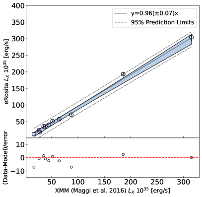
Figure 1: Comparison between the luminosity measured with eROSITA and the luminosity reported in Maggi et al. (2016) calculated using data from XMM-Newton, in the energy range $0.3-$8.0\text{\,}\mathrm{keV}$$. In the light blue region is shown the 95% confidence interval around the best fit line. The dashed line shows the 95% prediction lines around the best fit. The bottom pannel shows the residualt between the data and the best fit. From the plot the agreement between the luminosities of SNRs obtained by the two different instruments is evident.

3.2 Images

The eROSITA survey data are divided in separate sky tiles, which in total cover the entire sky. We used the eSASS package to generate a mosaic event list of the LMC by combining sky tiles includiung the LMC observed with TM1-TM4 and TM6.

We created event maps in three different energy bands: $0.2\mbox{--}$0.7\text{\,}\mathrm{keV}$$, $0.7\mbox{--}$1.1\text{\,}\mathrm{keV}$$, and $1.1\mbox{--}$5.0\text{\,}\mathrm{keV}$$, which are appropriate to detect and identify X-ray emission from SNRs (Kavanagh et al., 2016). We binned 80 physical pixels obtaining an image with a pixel size of 4$\arcsec/\mathrm{pixel}$, which corresponds to the on-axis resolution of the eROSITA telescopes.

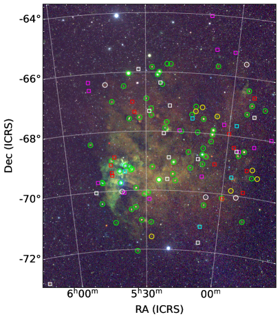
Figure 2: Exposure corrected three-colour image of the entire LMC observed by eROSITA during the eRASS:4. Red: $0.2\mbox{--}$0.7\text{\,}\mathrm{keV}$$, green: $0.7\mbox{--}$1.1\text{\,}\mathrm{keV}$$ and blue: $1.1\mbox{--}$5.0\text{\,}\mathrm{keV}$$. The coloured symbols indicate the positions of known SNRs and SNR candidates initially proposed in different wavelengths, while the shape of the symbols distinguishes the candidates (boxes) from the confirmed SNRs (circles). Green markers show known SNRs analysed with XMM-Newton data in Maggi et al. (2016), cyan markers radio candidates proposed by Bozzetto et al. (2017), magenta markers optical candidates proposed in Yew et al. (2021), red circles candidates proposed in Bozzetto et al. (2023) and yellow marks candidates confirmed in Kavanagh et al. (2022). White colour marks the positions of SNR candidates and SNRs proposed in this work.

The exposure map was obtained using the task expmap and the same binning and energy ranges as for the event maps, with vignetting correction applied. We divided the event map by the exposure map in order to acquire an exposure-corrected image. The final image was smoothed with a Gaussian kernel of $3$ pixels. Figure 2 shows the resulting three-colour image of the LMC for the three energy bands described above.

For the point source identification, we used the point source catalogue obtained by the eSASS team using eRASS:4. The pipeline to obtain such a catalogue is described in Merloni et al. (submitted). To exclude the point sources we selected sources in the catalogue with at least a detection likelihood $\texttt{DETLIKE}>10$ if the extension likelihood $\texttt{EXTLIKE}=0$, and $\texttt{DETLIKE}>20$ if the extent $\texttt{EXT}>0$. We excluded a circular region centred on the point sources with a radius of $28\arcsec$ which corresponds to the half energy width reported in the catalogue. We removed the corresponding events from the original mosaic event file and recreated an exposure-corrected image.The images shown in the paper are the original exposure corrected images. For the analysis we used the point subtracted images.

We have marked the positions of known SNRs and SNR candidates in the image: the known SNRs studied in the X-ray band using XMM-Newton data and Chandra data (Maggi et al., 2016; Maitra et al., 2019) are shown in green. In magenta, we highlight the SNRs and SNR candidates in the optical proposed by Yew et al. (2021) using the MCELS survey. In cyan, the radio candidates proposed in Bozzetto et al. (2017) are shown, while in red the new SNR candidates detected with the ASKAP telescope in the radio band (Bozzetto et al., 2023). In yellow we show the candidates confirmed in Kavanagh et al. (2022). Finally, in white we show the position of 15 new eROSITA sources detected for the first time in this work. The circles indicate the confirmed SNR in the LMC while the rectangles show the position of the remaining candidates. We can confirm three of the eROSITA candidate as SNRs based on multi-wavelength data as described in Sect. 4. The three-colour images of each SNR are shown in Appendix B and in Fig. 7.

3.3 Gaussian gradient magnitude filter

By visually inspecting the eROSITA LMC images we searched for new SNR candidates. To enhance the diffuse emission, we applied a Gaussian gradient magnitude (GGM) filter on the eRASS:4 images (Sanders et al., 2016). The filter calculates the magnitude of the gradient of an image using Gaussian derivatives. Firstly, the input image is smoothed with a Gaussian filter of a certain $\sigma$. Secondly, the derivative along the x- and y-axis is taken. The magnitude of the gradient is then determined by summing the squared derivatives under the square root. Where the intensity of the image changes rapidly over the pixels the magnitude has a greater value, which can be used to highlight regions of rapid change in intensity. Usually, the edges of objects are characterized by such a change in intensity over pixels, which will be shown as maxima in the filtered image. Therefore, the GGM filter can act as an edge detection algorithm. We are interested in edges of the shells of SNRs. The resulting image depends on the choice of $\sigma$ for the GGM filter, which is measured in pixels. For a certain $\sigma$ the filter will highlight the edges in the image with a certain pixel scale. Thus, we exploited various values of $\sigma$ ($\sigma$ = 1, 2, 4, 8, and 10 pixels) and combined the resulting filtered images into one. In order to reduce the noise resulting from point sources we applied the GGM on the point source subtracted count rate image.

We repeated the procedure described above for each energy band. The result of this technique is shown in Fig. 3. This image was useful to detect faint sources or, also to check if at the position of a known SNR candidate an edge structure is detectable. Finally, the spotted candidates were compared with the X-ray count rate image and images showing emission at other wavelengths as described in Sect. 4 and shown in Appendix B.

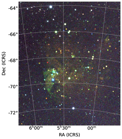
Figure 3: Gaussian Gradient Magnitude (GGM) filter applied eROSITA image after point sources were removed, showing the magnitude of the gradient of the input image. The filter is applied to each energy band separately and then composed into a three-colour image.

3.4 Hardness ratio

The relative faintness of the sample prevented us from performing a detailed spectral analysis for all sources. Therefore, we calculated the hardness ratio (HR) for a larger sample of SNRs and SNR candidates in our catalogue. We defined four energy bands soft $=0.3\mbox{--}$0.7\text{\,}\mathrm{keV}$$, medium $=0.7\mbox{--}$1.1\text{\,}\mathrm{keV}$$, hard $=1.1\mbox{--}$2.3\text{\,}\mathrm{keV}$$, harder $=2.3\mbox{--}$4.0\text{\,}\mathrm{keV}$$ and determined the net count rates in each energy band. We then computed three hardness ratios according to equation 1 for different combinations of energy levels:

$$\mathrm{HR}_{i}=\frac{R_{\text{i+1}}-R_{\text{i}}}{R_{\text{i+1}}+R_{\text{i}}}$$ (1)

where $R_{\text{i}}$ is the net count rate in each band.

However, due to the faintness of our sample we keep the sources with a net count rate greater $0.01$ cts $\mathrm{s}^{-1}$ in the energy band $0.2\mbox{--}$5.0\text{\,}\mathrm{keV}$$. Among them, we selected the sources with a net count rate greater than $0.001$ cts $\mathrm{s}^{-1}$ in each band (soft, medium, hard, and harder). We plotted $\mathrm{HR}_{1}-\mathrm{HR}_{2}$ and $\mathrm{HR}_{2}-\mathrm{HR}_{3}$ in Fig. 4 with SNR types from the classification proposed in Maggi et al. (2016). In the plot we also exclude the point with and error larger than $0.3$. The energy levels chosen for the HR calculation are sensible to different origins of the remnants, and therefore we expect to see a separation in the plots. We can also see that the source that have a secure classification are harder than the unclassified. This is because the well-secured classifications are the younger objects, which are brighter and have higher temperatures. Mature SNRs, which are dominated by the ISM emission, are colder with temperatures of $0.2-$0.3\text{\,}\mathrm{k}\mathrm{e}\mathrm{V}$$, and with low HR1, HR2. As the soft band is also affected strongly by absorption, the hardness ratios also depend more on the column density $\text{N}_{\text{H}}$. Thus unclassified candidates in those regions of the HR diagram cannot be classified only based on the HR diagrams. As type Ia SNe produce mostly iron, we expect a peak in the emission of type Ia SNRs around $1.0\text{\,}\mathrm{keV}$ due to the Fe-L complex.

In order to highlight the different HRs predicted by different models we assumed two model. The first a collisional ionisation equilibrium model (CIE) then a Non-ionisation equilibrium model (NEI). We assumed different temperatures for the two models and let the $\text{N}_{\text{H}}$ to vary from $0\ \unit{\per\squared}$ to $2.5\times 10^{22}\unit{\per\squared}$. In any model we assumed the abundances to be $0.5Z_{\odot}$.

We stress that although SNRs with different progenitors show different HRs we cannot determine the origin of the SNR by only considering the HR. To be able to classify the origin of an SNR, we need high-resolution spectra where different element abundances can be measured. In this work, we discuss the possible progenitor type by combining the HRs with information about the underlying stellar population at the location of the SNR.

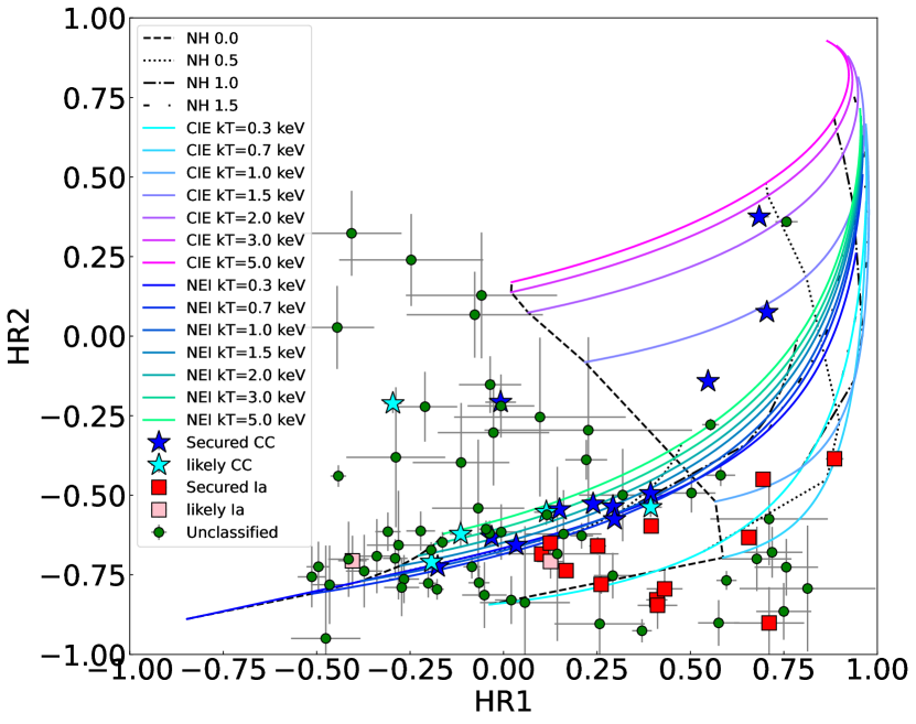
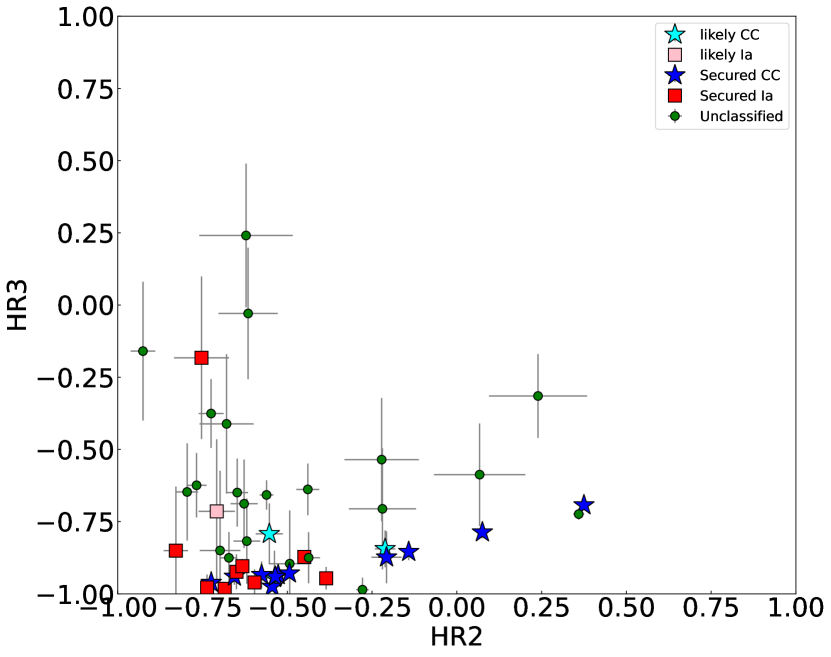
Figure 4: Hardness ratios of candidates and confirmed SNRs in our sample. The energy bands used to calculate HR1 are Soft: $0.3-$0.7\text{\,}\mathrm{k}\mathrm{e}\mathrm{V}$$ and Medium: $0.7-$1.1\text{\,}\mathrm{k}\mathrm{e}\mathrm{V}$$, while for HR2 the Hard: $1.1-$2.3\text{\,}\mathrm{k}\mathrm{e}\mathrm{V}$$, and for HR3 the Harder: $2.3-$4.0\text{\,}\mathrm{k}\mathrm{e}\mathrm{V}$$. The sources are separated according to the explosion type as reported in Maggi et al. (2016). The SNRs tend to be separated according to the progenitor of the remnant. The continuum lines describe the expected HRs values assuming different models. The NEI models are obtained assuming an ionisation time $\tau=10^{10}\,\unit{cm^{-3}}$, while for the CIE models we assumed $\tau=10^{13}\,\unit{cm^{-3}}$. Then for each model we varied $\text{N}_{\text{H}}$ in the range $0-2.5\times 10^{22}\,\unit{\per\squared}$. With the dashed, dot-dashed, and dotted line we highlight the regions with specific $\text{N}_{\text{H }}$.

4 Multi-wavelength analysis

Supernova remnants are multi-wavelength objects and can be observed from radio to X-rays, in some cases also in gamma-rays. Morphologically, SNRs have mainly bubble- or shell-like structures and can easily be confused with H II regions and planetary nebulae (PNe). To find new SNRs, a multi-wavelength investigation is mandatory. If we observe an X-ray source with a bubble- or shell-like structure we classify the object as an SNR candidate. To confirm whether the source is an actual SNR, we have to observe emission in at least one other band, either in optical or in radio. The details of the method are described in Hurley-Walker et al. (see Sect. 2.4 of 2019), Filipović et al. (2022) or Bozzetto et al. (2023).

In the optical, we look for an excess in the ratio of two emission line fluxes ${\mathrm{[{S\textsc{II}}]/H}\alpha}$. For ${\mathrm{[{S\textsc{II}}]/H}\alpha<0.4}$ the gas is photo-ionised, a process which typically occurs in H II regions around young and hot stars or in super-bubbles. For $\mathrm{[{S\textsc{II}}]/H}\alpha>0.4$ the ionisation is likely caused by a shock (Mathewson & Clarke, 1973; Dodorico et al., 1980; Fesen, 1984; Blair & Long, 1997; Matonick & Fesen, 1997; Dopita et al., 2010; Lee & Lee, 2014; Vucetic et al., 2019; Vučetić et al., 2019; Lin et al., 2020). The presence of a shock wave is a strong indication for the presence of an SNR. In the radio band, the presence of an SNR is usually identified by measuring the spectral index $\alpha$ defined as $S_{\nu}\propto\nu^{\alpha}$, where $S_{\nu}$ is the flux density and $\nu$ the frequency. For SNRs we expect $\alpha\sim-0.5$, which indicates non-thermal emission (Filipović et al., 1998; Guzmán et al., 2011).

4.1 Optical

To investigate the optical counterpart we use the MCELS data. The MCELS is very useful for studying the SNR as it provides us with narrow-band images from which we can derive the intensity of the emission lines.

Essential for the detection and classification of SNRs is the ratio ${\mathrm{[{S\textsc{II}}]/H}\alpha}$ as described above. The common ratio used to discriminate between H II regions and SNRs is $0.4$. This because behind the radiative shock we expect wild variety of ionisation states for the sulfur, as supperted by several radiative shock models (Raymond, 1979; Hartigan et al., 1987; Dopita & Sutherland, 1995; Allen et al., 2008). Accordingly with Long et al. (2018) for low surface bright objects, it is less obvious to distinguish between H II regions and SNRs. Studying the SNRs and SNR candidates in M33 Long et al. (2018) found that ${\mathrm{[{S\textsc{II}}]/H}\alpha}$ ratios can vary between $0.2-0.5$ for low surface brightness nebulae. For this reason, in this work, we use ${\mathrm{[{S\textsc{II}}]/H}\alpha>0.67}$ as a criterion to understand if the gas was ionised by shock waves. Even if the ${\mathrm{[{S\textsc{II}}]/H}\alpha}$ ratio is very useful to identify SNR it is a so-called second-order feature and has meaning only if the emission of H${\alpha}$ is significant. If the H${\alpha}$ emission is too low we can observe an artificial enhancement in the ${\mathrm{[{S\textsc{II}}]/H}\alpha}$ ratio.

4.2 Radio

From SNRs, we expect predominantly non-thermal emission in radio via synchrotron radiation. In young SNRs, synchrotron emission is also observed in the X-ray band. The more energetic electrons, emitting synchrotron radiation in X-rays, lose energy faster than the less energetic electrons, which will stay relativistic and emit in the radio band much longer. We used the public data from the ASKAP interferometry at $888$ MHz (Pennock et al., 2021). This image covers the entire LMC.

In order to highlight the non-thermal emission in this image we used the same approach as in Bozzetto et al. (2023) and in Ye et al. (1991). Where no supernova explosion occurred, we expect a correlation between the H${\alpha}$ emission and the radio continuum, as in these regions, we have thermal emission only. This is due to the fact that the free electrons that produce thermal radio emission via Bremsstrahlung are the same as those that recombine with the protons to produce the H${\alpha}$ lines. We can use this proportionality to highlight the non-thermal emission in the radio images. After subtracting a scaled H${\alpha}$ image from the radio continuum what remains is just the non-thermal emission. In order to subtract the optical image from the radio image, we need a normalization factor. This factor can be determined from the correlation between the pixel values in H${\alpha}$ and the radio continuum in the regions where we expect that the emission is just thermal. In order to measure the correlation, we selected different regions inside H II regions in the entire LMC. We measure the [S II]/H${\alpha}$ ratio and select only those regions with a ratio $<\ 0.4$ in order to be sure that there are no SNRs hidden inside the selected H II regions. We extracted the intensity of H${\alpha}$ and radio from the same physical region and compared the values. We performed a linear fit in the H$\alpha$-radio diagram and calculated the Pearson coefficient to evaluate the goodness of the fit. The slope of the plot is the normalization factor which can be used to normalize the H${\alpha}$ before subtracting it from the radio continuum. We averaged the different slopes using a weighted average using the Pearson coefficients as the weight.

In Fig. 5(b) we show the example of the H II region DEM-L140. Figure 5(a) shows the H${\alpha}$ emission, Fig. 5(b) shows the radio continuum of DEM-L140, and Fig. 5(c) shows the [S II]/H${\alpha}$ ratio. In order to avoid outliers which could contaminate the linear fit we recursively cleaned the data until the standard deviation of the pixel value vector stops to decrease.The linear relation and the linear fit are shown in Fig. 5(d). We adopted the average slope as the normalization factor. We scaled the H${\alpha}$ image and subtracted the scaled H${\alpha}$ emission from the radio-continuum emission. The H II regions used are: DEM-L111, DEM-L140, DEM-L194, DEM-L196,LHA-120-N44J, LHA-120-N70, MCELS-L401, N11, N44C, NGC-1899. From these H II regions, we selected several smaller regions and obtained a total of $61$ sub-regions. To calculate the average slope we keep just the region which shows a Pearson coefficient greater than $0.9$. Using this criterion we have a final number of $11$ regions that contribute to the averaged slope. In Table 1 we report the selected H II sub-regions used to calculate the average slope with the relative fitted slopes and the Pearson coefficients for each sub-region. At the end of the table, we give the final average slope used to normalize the H$\alpha$ emission. The error on the average slope was calculated using the formula to propagate the error on the weighted average:

$$\sigma=\frac{1}{\sum_{i}w_{i}}\sqrt{\sum_{i}(w_{i}\sigma_{i})^{2}},$$ (2)

where $w_{i}$ are the Pearson coefficients and $\sigma_{i}$ are the errors on the single fitted slope. The error on the single slope has been calculated using the python package used to fit the slope of the correlation scipy.optimize.curve_fit.

Table 1: H II regions used to calibrate the normalization factor for the H$\alpha$ images. The first column reports the name of the H II region used to extract the H$\alpha$ and radio pixel values. The second column indicates the fitted slope of the linear relation between radio and H$\alpha$. The third column documents the Pearson coefficient of the linear fit. The latter was used as a weighting factor in the calculation of the averaged normalization factor.

Region	Fitted Slope	Pearson coefficient
DEM-L140	$18549.7\pm 235.4$	$0.98$
LHA-120-N44J	$17533.2\pm 250.9$	$0.97$
LHA-120-N70 (a)	$18082.3\pm 212.8$	$0.95$
LHA-120-N70 (b)	$14955.2\pm 217.0$	$0.91$
LHA-120-N70 (c)	$14542.7\pm 181.2$	$0.93$
N11 (a)	$10443.16\pm 152.4$	$0.98$
N11 (b)	$10961.5\pm 394.4$	$0.91$
N11 (c)	$14975.1\pm 456.0$	$0.93$
N11 (d)	$17026.6\pm 505.1$	$0.93$
N11 (e)	$8690.2\pm 231.09$	$0.92$
N11 (f)	$16119.2\pm 209.27$	$0.99$
Average	$14751.7\pm 89.2$	$0.95$

After the subtraction of the scaled H$\alpha$ from the radio continuum image only the non-thermal radio emission remains. We used it to draw contours in the radio continuum images at 2, 3, and $5\sigma$ levels above the background to search for significant emission in an SNR.

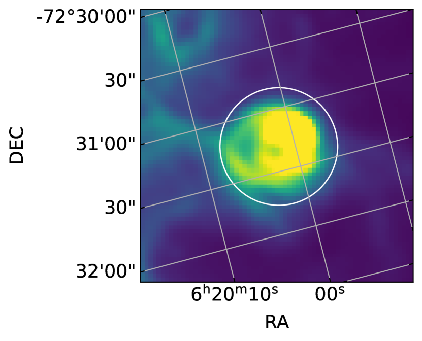
(a)

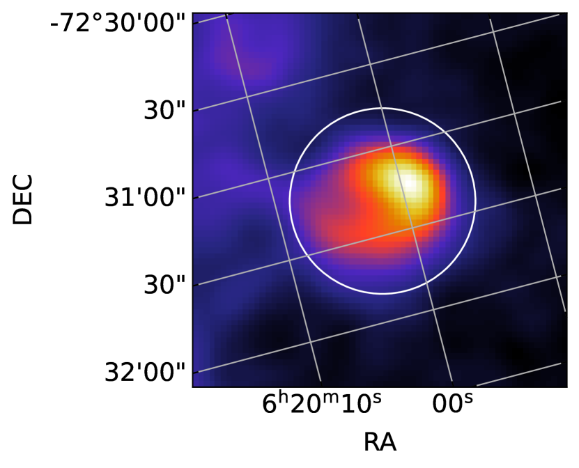
(b)

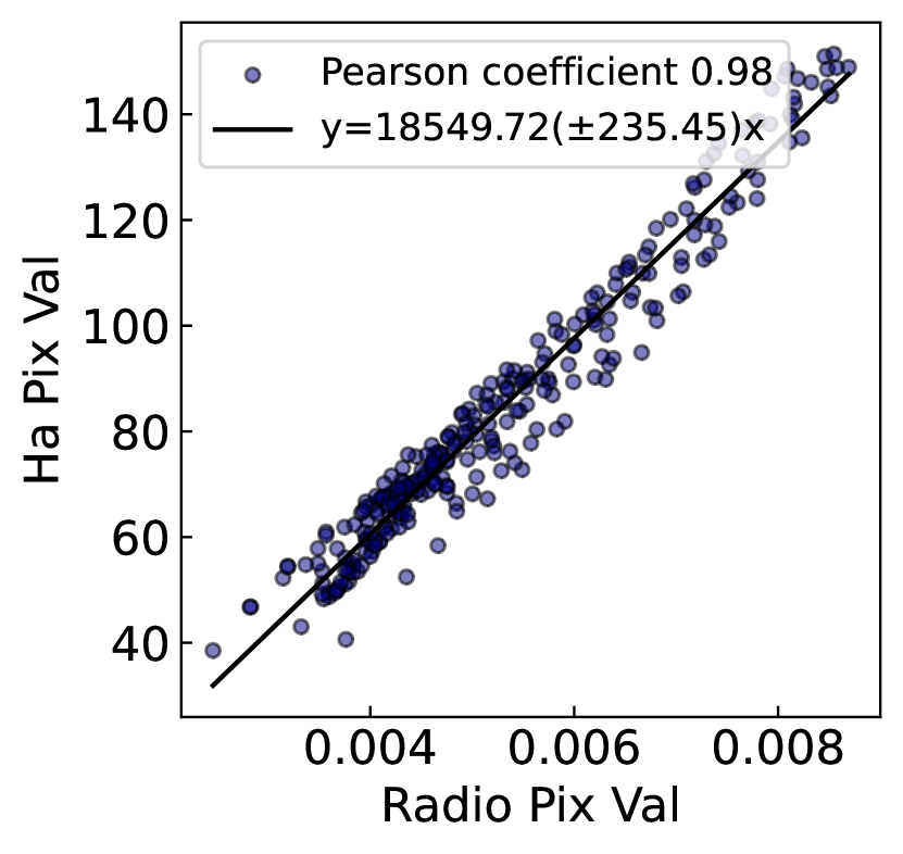
(d)

Figure 5: A subregion of the H II region DEM-L140 chosen to highlight the non-thermal emission in the radio images. In particular Fig. 5(a) and 5(b) show the emission of the selected region in H$\alpha$ and radio respectively. Figure 5(c) displays the image of the ${\mathrm{[{S\textsc{II}}]/H}\alpha}$ ratio. The latter image is used to ensure that the selected region is not affected by any SNR which would increase the ${\mathrm{[{S\textsc{II}}]/H}\alpha}$ ratio to values larger than $0.4$. In Fig. 5(d) the linear correlation between the H$\alpha$ and radio emission in the selected area is reported. The black solid line represents the best linear fit for this correlation.

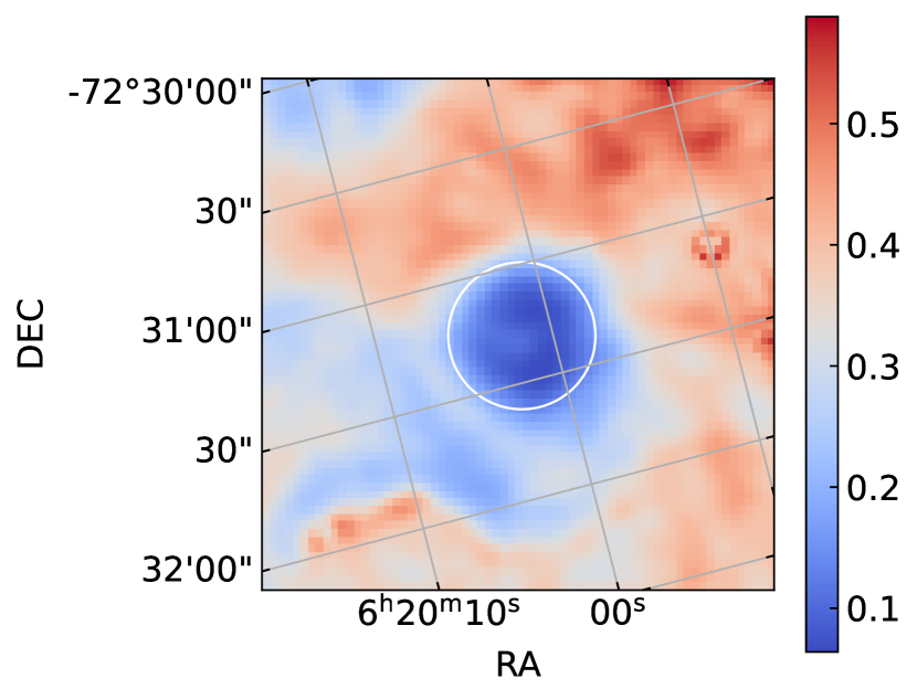
(c)

5 SFH-based progenitor classification

A necessary (but not sufficient) condition for a CC SNR is the presence of recent star formation (SF) activity near the SNR. In order to find the possible origin of SNRs and SNR candidates, we estimated the number of OB stars in the proximity of each source. We used the star formation history (SFH) values measured by Mazzi et al. (2021) using the near-infrared photometry from the VISTA survey of the Magellanic Clouds (VMC). The VMC data covers ${\sim}96\ \text{deg}^{2}$ and consists of infrared observations in the $Y$, $J$ and $K_{\text{s}}$ bands.

We calculated the SFH (Mazzi et al., 2021) around each source within a radius of $100\,\mathrm{pc}$. This corresponds to the maximal projected distance that a star with a typical velocity of $10\ \mathrm{km}\,\mathrm{s}^{-1}$ travel in $10^{7}\,\mathrm{yr}$. We measured the average star formation rate (SFR) in a time interval equal to the typical lifetime of a massive star for which we used $\log(t_{*}[\mathrm{yr}])=7.74$. Multiplying the average SFR with the time interval we obtained the total stellar mass formed in $10^{7}\,\mathrm{yr}$. A certain amount of the total stellar mass will be from the massive stars that are responsible for the CC explosions. To find the number of massive stars we used the imf python package, which creates a sample of stars with a mass distribution that follows a desired initial mass function (IMF). We assumed a Kroupa IMF (Kroupa, 2001) which is a good assumption for the LMC. We then counted the number of stars with $M_{*}>8\ M_{\odot}$ present in the sample. As this approach is based on sampling a mass distribution, we populated several samples for each SNR and averaged the number of massive stars ($N_{\text{OB}}$) obtained in the surroundings of each SNR. We stress that using this method we obtain the total number of massive stars created from $10^{7}\,\mathrm{yr}$ ago until now. Since $10^{7}\,\mathrm{yr}$ is the typical lifetime of a massive star, some of the massive stars we are counting have already died in a CC SN, so the total number of massive stars differs from the number of massive stars present in the surrounding of the SNRs today.

We repeated the same procedure to calculate the total number of stars. In this case, we calculated the average total stellar mass formed in the last $10^{10}\,\mathrm{yr}$. As described above we populated an IMF using the total mass of stars and counted the amount of stars with $M_{*}>0.08\ M_{\odot}$. In this way, we obtained the number of stars created in the interested region.

For each region, we calculated the fraction of massive stars over the total number of stars $f=N_{\text{OB}}/N_{\text{tot}}$. We want to use this ratio to roughly estimate the probability that an SNR that we observe could have been generated by a CC explosion. Therefore, to have a reference to compare $f$, we calculate the median value of the ratio $\bar{f}_{\text{Ia}}=(N_{\text{OB}}/N_{\text{tot}})_{\text{Ia}}$ for SNRs which were classified as secure type Ia SNR using spectral analysis (see Maggi et al., 2016, and references therein). We choose to use the median as best representative of the typical value for the massive star fraction of the Type Ia because the distribution is not Gaussian. We used the standard deviation as an estimate of the error $\delta_{\text{Ia}}$ on this ratio $\bar{f}_{\text{Ia}}$. If $f$ of a certain SNR or SNR candidate is significantly higher than $\bar{f}_{\text{Ia}}$, it indicates a high probability that an observed SNR has a CC origin. To evaluate whether this is the case we calculated the significance $S=\lvert f-\bar{f}_{\text{Ia}}\rvert/\delta_{\text{Ia}}$. Figure 6 shows the map of the significance $S$ in the LMC and Table 2 lists the significance values obtained for the eROSITA candidates and the eROSITA SNRs. Only two of the new sources have a significant difference above 3, which means that according to our analysis, they are likely CC SNRs.

Our analysis confirms the tendency for CC explosions to take place around H$\alpha$ emitting regions which show a high SFR. Therefore, CC SNRs are found around the star-forming region 30 Dor and at the bottom rim of the SGS LMC 4 where the SFR exhibits a peak (Schneider et al., 2018). Instead, SNIa tends to occur in the bar of the LMC. In Appendix A we show the SFH around the eROSITA SNR candidates. We discuss the plots in the subsections dedicated to each SNR and SNR candidate.

Table 2: Significance $S$ in the difference between the fraction of massive stars with respect to the total number of stars and the typical value of the same fraction calculated for thermonuclear SNRs. The list include only the new eROSITA candidates and SNRs. The nomenclature for the candidates follow the eROSITA convention, while the confirmed SNR are called using the SNR convention. The full calculation is explained in Sect. 5.

Source ID	$S$	CC origin
4eRASSU J045145.7$-$671724	0.12	Unlikely
MCSNR J0456–6533	1.63	Unlikely
4eRASSU J045625.5$-$683052	0.51	Unlikely
MCSNR J0506–7009	0.04	Unlikely
4eRASSU J050750.8$-$714241	0.33	Unlikely
4eRASSU J051028.3$-$685329	0.03	Unlikely
4eRASSU J052136.6$-$670741	0.81	Unlikely
4eRASSU J052126.5$-$685245	0.04	Unlikely
4eRASSU J052148.7$-$693649	0.32	Unlikely
4eRASSU J052330.7$-$680400	5.45	Likely
4eRASSU J052502.7$-$662125	1.51	Unlikely
4eRASSU J053224.5$-$655411	2.03	Unlikely
4eRASSU J052849.7$-$671913	5.87	Likely
MCSNR J0543–6624	2.45	Unlikely
4eRASSU J054949.7$-$700145	0.76	Unlikely
4eRASSU J061438.1$-$725112	0.03	Unlikely

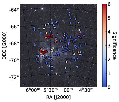
Figure 6: Distribution of the significance $S$ in the difference between the fraction $N_{\text{OB}}/N_{\text{tot}}$ for secure Ia and all SNR. The calculation of $S$ is described in Sect. 5. The sources with high significance present a higher fraction of massive stars with respect to the total number of stars. The higher fraction is associated with a higher probability that the SNR or the SNR candidate has a CC origin. The triangle shows the positions of the eROSITA candidates and eROSITA SNRs, which are listed in Table 2.

6 Classifications of candidates

In order to understand if there is emission associated with an SNR, we compared the X-ray, optical and radio images. We show the comparisons in Appendix B. On the left side, we show the three-colour eROSITA image of the source in the bands $0.2\mbox{--}0.7$, $0.7\mbox{--}1.1$, and $1.1\mbox{--}$5.0\text{\,}\mathrm{keV}$$. The contours show the region in the event map with emission $1\sigma$, $2\sigma$, and $3\sigma$ above the background. The second image is the GGM image of the X-ray emission, described in Sect. 3.3. The third panel shows the MCELS image where we can see the emission of H${\alpha}$, [S II], and [O III]. The contours in the optical image represent the [S II]/H${}_{\alpha}>0.67$. In the right panel, we show the radio continuum image from the ASKAP survey of the LMC at $888\,\mathrm{MHz}$. The contours indicate the non-thermal emission at $2\sigma$, $3\sigma$, and $5\sigma$ above the background as described in Sect. 4.2.

6.1 SNRs discovered and confirmed with eROSITA

The new SNRs first found in eROSITA and then confirmed thanks to the multiwavelength analysis are described below. The report the name of each source following the SNR convention while in brackets we report the name following the eROSITA convention. The list of the eROSITA confirmed SNR is listed in Table 6.

MCSNR J0456–6533 (4eRASSU J045650.7–653244):

this source was seen for the first time with eROSITA (see Fig. 7). The X-ray emission has a circular shape with a soft shell surrounding a central region with harder emission. Even though the $3\sigma$ detection is present just in a small portion of the source we can confirm the source as an SNR thanks to the XMM-Newton follow-up observation described in Sect. 7. In the optical images, we can clearly see an [O III] shell with a small enhancement of [S II]/H${}_{\alpha}>0.67$ in the north of the shell. Also in the radio image, a faint emission is correlated with the optical shell, which surrounds the X-ray emission. Parts of the radio shell show non-thermal emission. We can thus confirm the source as an SNR. The source is shown in Fig. 7. In Fig. 7 we show the plot of the SFH, in which there is an enhancement of star formation around $10^{9}\,\mathrm{yr}$ ago. The recent SFR has large uncertainty which prevents us from arguing for a recent star formation activity. Combining the information from the spectral analysis, discussed in Sect. 7 and the SFH we suggest a type Ia origin for the remnant.

MCSNR J0506–7009 (4eRASSU J050615.8–700920):

The source is located next to a molecular cloud known as LMC N J0506–7010 (Fukui et al., 2008). It has a relatively small size of 98″  $\times$ 72″. The source shows a peak of emission in the energy band of $0.7\mbox{--}1.1\,\mathrm{keV}$.The image shows a clear $3\sigma$ detection. In the optical band, we can see a faint shell of [S II] and a strong enhancement of [S II]/H${\alpha}$ especially in the northeast. In the radio band, the continuum emission is very faint but with a non-thermal emission in the northeast, with the contours suggesting a semi-shell structure. We can confidently confirm the source as a new SNR. The source is shown in Fig. 7. The SFH in Fig. 7 shows a peak around $10^{9}\,\mathrm{yr}$ ago, but also lower peak around $10^{8}\,\mathrm{yr}$ ago. The SFH does not show a particular activity in the recent past. The $\mathrm{HR}_{1}=0.72\pm 0.08$ and $\mathrm{HR}_{2}=-0.68\pm 0.08$ suggest that the source is located in the region populated by type Ia source in the $\mathrm{HR}_{1}-\mathrm{HR}_{2}$ diagram. Combining the HRs, the colour of the image, and the SFH we suggest a thermonuclear progenitor for the SNR.

MCSNR J0543–6624 (4eRASSU J054348.6–662351):

The source shows a soft X-ray emission with an irregular rectangular shape (Fig. 7). The X-rays show $3\sigma$ emission in the centre of the source. In the optical band, we can see a similar elliptical shape embedded in a H II region with an enhancement of the ratio [S II]/H${\alpha}$. In addition, there is a shell-like structure around the source in the optical and radio images. In radio, we do not detect any clear non-thermal emission. The SFH (Fig. 7) peaks at $10^{7}$ yrs ago, which suggests a possible CC origin of the remnant. Also in the HR diagrams, the source is in the region typical for CC SNRs. The CC origin is in agreement with the fact that the source is embedded in a H II region. Combining the X-ray and the optical information we can confirm the source as an SNR.

ı/ȷin J0614-7251/4eRASSU J061438.1–725112,J0456-6533/MCSNR J0456–6533,J0506-7009/MCSNR J0506–7009,J0543-6624/MCSNR J0543–6624

(a) ȷ

Figure 7: For each source we show the eROSITA count rate three-colour image (left) with red: $0.2\mbox{--}$0.7\text{\,}\mathrm{keV}$$, green: $0.7\mbox{--}$1.1\text{\,}\mathrm{keV}$$, and blue: $1.1\mbox{--}$5.0\text{\,}\mathrm{keV}$$, the GGM filter image (see Sect. 3.3) applied to the eROSITA count rate (middle left), the MCELS survey three-colour image (middle right) with red: H$\alpha$, green: [S II], and blue: [O III], and the ASKAP radio continuum (right) in the upper panel. The cyan (red) contours in the eROSITA three-colour image show the detection at 1 and $2\sigma\ (3\sigma)$ over the background in the energy band $0.2\mbox{--}$1.1\text{\,}\mathrm{keV}$$. The contours in the optical image represent [S II]/H$\alpha>0.67$. The contours in the radio image show the non-thermal emission calculated as described in Sect. 4.2. In the lower panel we show the SFH as measured in Mazzi et al. (2021).

6.2 Previous candidate from ROSAT and MCELS confirmed with eROSITA

MCSNR J0454–7003:

The candidate was proposed by Yew et al. (2021) as an optical SNR candidate. The source is located on the southeast edge of the H II region LHA 120-N 185 (Davies et al., 1976; Pellegrini et al., 2012). In the optical band, the candidate shows a circular structure where the emission is dominated by [S II] and H${\alpha}$. Inside this emission, we can measure an enhancement of the ratio [S II]/H${\alpha}$. In our radio image, we can not detect any particular structure. In X-rays, there is some diffuse emission in the H II region and some emission at the position of the optical SNR candidate. Since we have $3\sigma$ detection and [S II]/H${\alpha}>0.67$ we consider this source as a confirmed SNR. The source is shown in Fig. LABEL:J0454-7003.

MCSNR J0539–7001:

This X-ray source was detected in the ROSAT survey Haberl & Pietsch (1999a) and classified as an SNR candidate. In the radio band, there is a point source almost at the centre of the SNR candidate, which can be seen in the ASKAP images (Fig. LABEL:J0539-7001). In Bozzetto et al. (2017) a spectral index of $\alpha=-0.47$ was measured. In the eROSITA three-colour image, the SNR appears as a bright elongated source in green indicating a peak in the emission in the medium energy band, probably due to Fe-L emission. This feature suggests a possible thermonuclear origin of the remnant, which is also indicated by its position in the HR diagrams shown in Fig. 4 with $\mathrm{HR}_{1}=0.60\pm 0.03$, $\mathrm{HR}_{2}=-0.77\pm 0.03$, and $\mathrm{HR}_{3}=-0.62\pm 0.11$. The source is clearly detected with $3\sigma$ confidence. Combining all the information we can confirm this source as an SNR.

6.3 SNR candidates detected with eROSITA

In the eROSITA data, we detected 16 new diffuse sources in the X-ray images. Among them, we are able to confirm three as SNRs as presented in Sect. 6.1. In the following section, we present the 13 new SNR candidates detected with eROSITA for the first time. We report the name following the eROSITA convention and in bracket the name as usually used in the SNRs catalogues. The list of the eROSITA candidates is reported in Table 8

4eRASSU J045145.7–671724 (J0451–6717):

This candidate SNR might be associated with a radio pulsar detected by Manchester et al. (2006) using the Parkes radio telescope. The properties of the radio pulsar, including its position, are still highly uncertain. In our radio images, we can see a point source inside J0451–6717, which can be associated with the pulsar, but further observations to measure the pulse period are required for confirmation. In the optical, we can clearly see an elongated shell structure visible in H${\alpha}$, where partially the [S II]/H${\alpha}$ ratio is higher than $0.67$. In the X-ray images, we can see a diffuse emission, which correlates with the optical emission. Also in the GGM image, we can clearly see an edge with elliptical shape associated with the source. The region was observed with XMM-Newton but the candidate is located at the rim of the field of view, which prevented a previous detection. In the eROSITA images, there is no significant detection, only a $2\sigma$ detection in the north. We can also detect a small portion of the remnant which is detected with $3\sigma$ confidence. Since the $3\sigma$ is a very small portion we conservatively keep the source as an SNR candidate. Recently, this source was accepted for an XMM-Newton follow-up observation. With a deeper observation we will be able to further constrain the true nature of this object. The source is shown in Fig. LABEL:J0451-6717.

4eRASSU J045625.5–683052 (J0456–6830):

This source was identified for the first time in the eROSITA survey. In the X-ray three-colour image in Fig. LABEL:J0456-6830, it is seen as a diffuse green emission, which means that the emission peaks at around $1$ keV. Even if the source is relatively faint with a net count rate of $0.029\pm 0.007$ photons $\mathrm{s}^{-1}$, it is clearly visible in X-rays. The brightest part is on the southeast, as the $1\sigma$ contour shows. The source is relatively compact with a diameter of about $160\text{\,}\arcsec$ and has a circular shape. Also, the GGM image shows the presence of a diffuse emission. In the optical band, there is no compact emission clearly related to the candidate, but it is surrounded by a larger structure dominated by [S II]. No enhancement of [S II]/H$\alpha$ is visible. Neither in the radio continuum nor in the non-thermal component any emission is detectable. Therefore, the source remains a candidate. Figure LABEL:J0456-6830 shows the SFH within 100 pc around the centre of the candidate, which shows a relatively high and constant star formation activity from $10^{9}$ to $10^{8}\,\mathrm{yr}$ ago. The HRs and the colour of the image suggest a possible thermonuclear origin.

4eRASSU J050750.8$-$714241 (J0507–7143):

The source is shown in Fig. LABEL:J0507-7143. From its green colour in the three-colour image, we can conclude that the peak of the emission is at around $1.0\text{\,}\mathrm{keV}$. The presence of a diffuse source is confirmed by the GGM image. The source is relatively faint in the X-ray band with a count rate of $0.07\pm 0.01$ [$\mathrm{photons}\,\mathrm{s}^{-1}$]. We do not see any emission in the optical or in the radio band. In the radio image, there is a non-thermal source in the north which is due to an AGN in the background. The same AGN is visible as a point source in the X-ray image. We propose this source as an SNR candidate. In Fig. LABEL:J0507-7143 we show the SFH around the SNR candidate, which has a peak between $10^{9}$ and $10^{10}\,\mathrm{yr}$ ago. The region around the candidate did not face a recent SF activity. From the X-ray colour of the SNR candidate and the SFH, we can argue for a type Ia origin.

4eRASSU J051028.3–685329 (J0510–6853):

This source is located next to a molecular cloud [WHO2011] C173 (Wong et al., 2011). The source presents a faint X-ray emission which is also clearly seen in the GGM image. In the optical band, we can see a shell structure in the east with an enhancement of H${\alpha}$, [S II], and [O III]. The central region shows a filamentary emission bright in [S II]. There is no enhancement of [S II]/H${\alpha}$. Also in the radio image, we can see a shell structure in the east, with an enhancement of non-thermal emission. The source is shown in Fig. LABEL:J0510-6853. The SFH in Fig. LABEL:J0510-6853 shows no recent star formation. The hardness ratios $\mathrm{HR}_{1}=-0.21\pm 0.09$ and $\mathrm{HR}_{2}=-0.22\pm 0.11$ correspond to values characteristic of CC SNR (see Fig. 4). Therefore, despite the SFH, we can not rule out the CC scenario. Since no X-ray is detected at the $3\sigma$ level, the source is classified as a candidate.

4eRASSU J052136.6–670741 (J0521–6707):

The source is shown in Fig. LABEL:J0521-6707. From the eROSITA image we can observe a very faint diffuse with a net count rate of $0.09\pm 0.01[cts/s]$. The GGM image help us to discriminate the presence of an edge on the West part of the source. In the optical imge we detect an enhancement of [S II]/H${\alpha}>0.67$ in a the inner part of the shell, indicating that a possible shock occurred. In the radio image there is a point source detected by Filipovic et al. (1995) with the catalogue name B0521–6710 at 4.75 GHz, and by Marx et al. (1997) with the name MDM 15 and detected at 2.4 GHz. In the later paper they measure a spectral index of $-0.3$. No diffuse emission can be observed in the radio images. The SFH around the source, shown in Fig. LABEL:J0521-6707 indicates two relative peaks between $10^{7}-10^{8}$ years ago. The absence of the $3\sigma$ detection prevents us from confirming the source as an SNR, and it is classified as a candidate.

4eRASSU J052126.5–685245 (J0521–6853):

The source was detected in the ROSAT survey (Haberl & Pietsch, 1999b). In the eROSITA image, it is visible at $1\sigma$ level despite the source being located in a relatively bright environment. From the eROSITA images, the extent of the source is not clearly visible. Also, the GGM shows an enhancement of the emission relative to the surroundings. At the same location there is a diffuse emission in the optical image with emission from H$\alpha$, [S II], and [O III]. There is a small bright region in the centre with a diameter of about $21\text{\,}\arcsec$, embedded in a larger structure. No [S II]/H$\alpha$ enhancement is found inside the source even though there are some regions with [S II]/H$\alpha$ $>0.67$ in the surroundings. In the radio band, there is no non-thermal emission related to the candidate, but a very faint continuum emission is seen with a larger elongated structure extending to the north. This filamentary emission is large and non-thermal. The source is shown in Fig. LABEL:J0521-6853. The SFH around the source, shown in Fig. LABEL:J0521-6853 indicates no recent star formation activity. From the X-ray colour and the SFH, the source is likely not associated with a CC supernova. The absence of the $3\sigma$ detection prevents us from confirming the source as an SNR, and it is classified as a candidate.

4eRASSUJ052148.7–693649 (J0521–6936):

The source was identified for the first time with eROSITA probably because it is located in a region where the surrounding is bright in X-rays. The emission is brighter in the north. It peaks at around $1$ keV as the green colour suggests. The GGM image highlights the structure that is visible in X-rays. A very small region with $3\sigma$ emission can be observed in the northern part. In the optical image, the source is surrounded by diffuse emission in the east and the south with only small regions with [S II]/H$\alpha>0.67$. The X-ray peak correlates with a bubble-like structure in optical. In the radio image, we can not see any structure that can be related to the X-ray source. The source is shown in Fig. LABEL:J0521-6936. The SFH in Fig. LABEL:J0521-6936 indicates two relatively recent peaks around $4\times 10^{7}\,\mathrm{yr}$ and $10^{7}\,\mathrm{yr}$ ago. The calculated fraction of massive stars with respect to the total number of stars (see Sect. 5) suggests that the probability of a CC origin is very low ($S=0.020$). The low significance of the detection in the X-ray band prevents us from confirming the source as an SNR, and it remains a candidate.

4eRASSUJ052330.7–680400 (J0523–6804):

the X-ray images show a circular object with a radius of ${\sim}$ $116.4\text{\,}\arcsec$. Also, the GGM shows the circular edge of the source. We do not observe any emission in the optical band. While in the radio image, we can see an enhancement of the non-thermal emission, especially in the South. Unfortunately, we can not detect any $3\sigma$ detection. A deeper observation is needed to confirm the significance of the source. The source is shown in Fig. LABEL:J0523-6804. The $\mathrm{HR}_{1}=0.71\pm 0.16$ and $\mathrm{HR}_{2}=-0.57\pm 0.14$ locate the source in the region of $\mathrm{HR}_{1}-\mathrm{HR}_{2}$ (Fig. 4) populated by thermonuclear SNR. Also, the green colour in the X-ray image shows a peak in the emission around 1 keV typical of thermonuclear origin. Figure LABEL:J0523-6804 shows the SFH around the source. From the SFH we can observe a peak in the recent past around $10^{6}\,\mathrm{yr}$. This star formation activity would be compatible with a possible CC origin but from the position of the source in the HR diagram 4 and from the colour we propose the candidate to originate from a SNIa. The absence of a $3\sigma$ detection in the image prevents us from confirming the source as an SNR. For this reason, we propose this source as an SNR candidate.

4eRASSUJ052502.7–662125 (J0525–6621):

The source appears to have an irregular shape in the X-ray images, with a softer emission in the northeast (see Fig. LABEL:J0525-6621). There is some $3\sigma$ emission inside the source, but its distribution is not sufficient to confirm the source as an SNR. In the GGM image, we can observe a clearly enhanced edge. In the optical image, we can see a strong enhancement of [S II]/H${}_{\alpha}>0.67$ while in the radio image, we can observe a complex environment where the emission appears to be non-thermal. We can not clearly see a structure in the radio emission that correlates with the X-ray or the optical emission. The HRs of the source indicate a type Ia SNR (see Fig. 4). From the SFH in Fig. LABEL:J0525-6621 we can see a quite constant star formation activity from $10^{9}$ until today with a relative peak between $10^{8}\mbox{--}10^{7}\,\mathrm{yr}$ ago. We propose this source as a candidate.

4eRASSU J052849.7–671913 (J0528–6719):

The source presents a soft diffuse emission between $0.2\mbox{--}0.7\,\mathrm{keV}$ and thus appears red in the eROSITA images (Fig. LABEL:J0528-6719). In X-rays, it has a half-shell structure in the south, which is also visible in the GGM image. There is no emission that can be related to the X-ray source, neither in the optical nor in the radio. The SFH LABEL:J0528-6719 has a recent peak, which is compatible with a CC progenitor. The fraction of massive stars with respect to the total number of stars is significantly higher than the typical fraction for type Ia SNR (see Sect. 5) suggesting a CC origin for this candidate.

4eRASSU J053224.5$-$655411 (J0532–6554):

The source was detected in the ROSAT data by Haberl & Pietsch (1999b). Its ROSAT HRs suggested that it could be an AGN, SNR, or an X-ray binary. In the eROSITA images (Fig. LABEL:J0532-6554) the source shows a diffuse emission with count rate of $0.068\pm 0.005\,[\mathrm{counts}\,\mathrm{s}^{-1}]$ and $\mathrm{HR}_{1}=0.22\pm 0.05$, $\mathrm{HR}_{2}=0.39\pm 0.06$. The contours in the X-ray image show a $3\sigma$ emission. No particular structure can be observed in the optical or radio image. For this reason, we propose the source to be a candidate. The SFH in Fig. LABEL:J0532-6554 shows a recent increase in the star formation activity. The fraction of massive stars with respect to total stars created in the surrounding of the candidate shows an excess, which is nevertheless not significant enough to suggest a CC origin (see Sect. 5). This source is a candidate.

4eRASSU J054949.7–700145 (J0549–7001):

This source has an elongated shape in the northeast-southwest direction with a brighter emission in the southwest (Fig. LABEL:J0549-7001). The source is relatively bright with count rates of $0.062\pm 0.007\,[\mathrm{counts}\,\mathrm{s}^{-1}]$. The $1\sigma$ and $2\sigma$ contours follow the diffuse structure and small portions inside have detection with significance above $3\sigma$. In the optical band, the region presents a complex filamentary emission, where it is not clear if any structure can be related to the candidate. No enhancement in [S II]/H$\alpha$ ratio is observed. In radio, there is no emission associated with the source either. The SFH in Fig. LABEL:J0549-7001 shows a small peak at around $5\times 10^{6}$ yr ago. Nevertheless, this source is probably a thermonuclear SN candidate due to its colour and the star number fraction value (see Sect. 5).

4eRASSU J061438.1–725112 (J0614–7251):

This source is of particular interest as it is not located in the LMC but far out in the southeast, most likely inside the Magellanic Bridge (MB). The source was spotted in the eROSITA images because appear relatively bright with an approximately spherical shape. The region is not covered by the MCELS survey, therefore we do not have any optical data. The region was covered in the ASKAP survey of the LMC, but it is on the edge of the image where the radio sensitivity is lower and does not allow us to detect anything in the radio band. In X-ray, the source appears relatively bright and has a spherical shape, with a red ring of soft X-rays in the east. The inner part appears slightly harder with an orange colour. The source shows a prominent emission above the $3\sigma$ level (see red contours in Fig. 7). The net counts rate is $0.26\pm 0.01$ [photons $\mathrm{s}^{-1}$]. From the SFH in Fig. 7 we can see that there are no particularly recent peaks in star formation, which would rule out the CC origin for this SNR candidate. Also, the apparent regular shape is a suggestion that the source could have originated from a Type Ia SN (Lopez et al., 2011, 2009). Interestingly, the HR diagram suggests that the source might be related to a CC SN. Further investigations are needed to correctly classify the origin of the SNR candidate. We stress the peculiarity of the spatial location of the source, which might be an isolated SNR in the MB. If this is confirmed it would be the first SNR detected in the MB. The lack of multi-wavelength information does not allow us to confirm the source as an SNR, but it remains a very promising SNR candidate.

6.4 Known SNRs not included in Maggi et al. (2016) and detected with eROSITA

MCSNR J0447–6918:

The source was recently confirmed by Kavanagh et al. (2022) using XMM-Newton data. The source was a radio candidate proposed by Bozzetto et al. (2017). As shown in Fig. LABEL:J0447-6918 the remnant presents a diffuse emission in the radio continuum. We detect non-thermal emission, especially coming from the centre of the source. In the optical band, we can observe a half-ring structure in the south with high ${\mathrm{[{S\textsc{II}}]/H}\alpha}$. There is some additional filamentary emission which extends from the inner part of the shell to the northeast. The optical emission correlates with the diffuse radio emission. In X-rays, we also detect an elongated faint emission, which is more visible using the GGM filter and it agrees with the shell seen in the optical and radio images.

MCSNR J0449–6903:

This source was another radio candidate proposed by Bozzetto et al. (2017) and confirmed by Kavanagh et al. (2022). In radio, the source presents a prominent diffuse emission. Figure LABEL:J0449-6903 shows that there is a strong non-thermal emission which correlates with the entire diffuse emission. In the optical, there is a faint shell of [O III], where the interior has an enhancement of ${\mathrm{[{S\textsc{II}}]/H}\alpha}$. Neither in the eROSITA images nor in the GGM image we can detect any particular emission.

MCSNR J0456–6950:

This is another radio candidate (Bozzetto et al., 2017) confirmed as an SNR by Kavanagh et al. (2022). As shown in Fig. LABEL:J0456-6950 the radio image presents a diffuse spherical emission with the presence of non-thermal emission in the entire remnant. In the optical image, no clear emission can be associated with the remnant. In the eROSITA images, we can detect a diffuse soft circular emission.

MCSNR J0504–6723:

This remnant was proposed as an X-ray candidate by Haberl & Pietsch (1999a) and confirmed by Kavanagh et al. (2022). Fig. LABEL:J0504-6723 shows that also in the eROSITA images the source appears as a bright diffuse emission with a peak at around $1.0$ keV. In radio we do not detect any non-thermal emission and the continuum does not show a structure which can be connected to the remnant. In the optical image, we can clearly see an enhancement of ${\mathrm{[{S\textsc{II}}]/H}\alpha}$ ratio, especially in the north. In the rest of the region, we can see filaments of H$\alpha$ and [S II].

MCSNR J0506–6815:

This source was found by Bozzetto et al. (2023) and confirmed as an SNR in the same study. They measured a spectral index of $\alpha\sim-0.47$ and used an XMM-Newton observation, in which soft X-ray emission was detected. There is a clear circular emission in the radio with a non-thermal component. Also in the optical band, a clear shell is visible, which correlates with the radio emission. The X-ray emission is also clearly visible in the eROSITA data. The source is shown in Fig. LABEL:J0506-6815.

MCSNR J0507–6847:

The source was studied by Chu et al. (2000) using ROSAT data. In Fig. LABEL:J0507-6847 we can see that in X-rays there is a large elliptical shell with a point source at its centre. The SNR is associated with the high mass X-ray binary pulsar XMMU J050722.1–684758 (Maitra et al., 2021). The SNR presents an enhancement of ${\mathrm{[{S\textsc{II}}]/H}\alpha}$ in the north. Also, the radio continuum shows a faint shell structure associated with the SNR.

MCSNR J0510–6708:

Bozzetto et al. (2017) proposed the source as a radio candidate in particular because of the presence of a compact radio source in the centre of the emission. The source was then confirmed as an SNR by Kavanagh et al. (2022). As shown in Fig. LABEL:J0510-6708 one can only see the point source in the radio image. In the optical images, there is a faint circular structure where the emission is mainly due to [S II]. Inside the diffuse emission, the ratio is [S II]/H$\alpha>0.67$ which suggests that the gas has been heated by a shock. In the eROSITA images we can see a very faint diffuse emission with a count rate of $0.003\pm 0.08$ [cts $\mathrm{s}^{-1}$] but no significant detection.

MCSNR J0512–6716:

The source was proposed as a radio candidate (Bozzetto et al., 2017) and was recently confirmed as an SNR by Kavanagh et al. (2022). We show the images of the remnant in Fig. LABEL:J0512-6716. In the radio image, there is a diffuse elliptical emission with a brighter half-shell in the southeast. The contours in the image reveal that the emission from the bright shell is strongly non-thermal. In the optical images, we can see several filaments and a half shell of [O III], which correlates with the radio shell. No enhancement of [S II]/H$\alpha$ can be seen in the MCELS images. The eROSITA images show a diffuse soft emission.

MCSNR J0513–6724:

This source was proposed as a radio candidate and was confirmed as an SNR by Maitra et al. (2019) using XMM-Newton data. The source is clearly visible in the radio band as a diffuse emission with significant non-thermal emission. In the optical band, we can see a faint shell structure which overlaps with the radio emission. In the eROSITA image we can see a $3\sigma$ detection at the same position of the radio non-thermal emission. The source is shown in Fig. LABEL:J0513-6724.

MCSNR J0522–6543:

The source was proposed and confirmed as a bona-fide SNR by Bozzetto et al. (2023) with radio observation. In radio, there is a diffuse emission with a bright non-thermal point source roughly at the centre of the diffuse emission. The optical emission correlates with the radio emission with high [O III] emission in the interior. Bozzetto et al. (2023) measured a spectral index in the radio of $\alpha=-0.51\pm 0.05$ for the entire structure while for the point source, they measured a steeper photon index of $\alpha=-1.00\pm 0.04$. They argued that most likely the point source is a background AGN. In our X-ray images, we are not able to see the diffuse emission related to the SNR or any counterpart of the AGN. The source is shown in Fig. LABEL:J0522-6543.

MCSNR J0522–6740:

The SNR was proposed by Yew et al. (2021) and confirmed in the same paper using XMM-Newton data. In the optical band we can see a almost complete shell structure especially from [S II]. In the eROSITA image we can detect a $1\sigma$ emission which define a extended source which correlate with the optical emission. Small regions of $3\sigma$ can be observed with eROSITA. In the radio continuum we can not observe any particular emission. The source is shown in Fig. LABEL:J0522-6740.

MCSNR J0527–7134:

It is another radio candidate (Bozzetto et al., 2017), which was confirmed by Kavanagh et al. (2022). In Fig. LABEL:J0527-7134 we can clearly see a diffuse non-thermal emission in the radio band, while in the optical images, we see a compact circular structure where [S II]/H$\alpha>0.67$. In the eROSITA images, we can clearly see a diffuse emission with a clump of soft emission roughly at the centre.

MCSNR J0529–7004:

This optical candidate suggested by Yew et al. (2021) was confirmed as an SNR by Sasaki et al. (2022) using eROSITA data of the calibration and performance verification phase of the telescopes. In the MCELS images, we can see a shell structure that correlates with a faint radio emission (Fig. LABEL:J0529-7004). In our eROSITA images, we can see a bright extended structure in the interiors with a net count rate of $0.24\pm 0.02$ photons $\mathrm{s}^{-1}$.

MCSNR J0542–7104:

This optical candidate suggested by Yew et al. (2021) was confirmed in the same work using also XMM-Newton data. In the MCELS images, we can see a half shell structure with an enhancement of [S II]/H $\alpha$ to the East (Fig. LABEL:J0542-7104). In our eROSITA images, we can see a bright extended structure with a peak around $1\text{\,}\mathrm{k}\mathrm{e}\mathrm{V}$. We can detect some $3\sigma$ emission.

6.5 Previous candidates which remain candidates

J0444–6758:

This source was proposed as a candidate in Yew et al. (2021). From the optical images, we can see a relatively compact emission from [O III] surrounded by an H${\alpha}$ shell. At the centre, we can see, from the contours, that the [S II]/H${\alpha}$ ratio is higher than $0.67$. In our radio image, we cannot distinguish any diffuse structure related to the candidate. In the eROSITA images, we cannot see enough X-ray emission to confirm this candidate as an SNR. Therefore, the source stays a candidate. The source is shown in Fig. LABEL:J0444-6758.

J0450–6818:

This source was also proposed as a candidate in Yew et al. (2021) in the optical band. Indeed in the MCELS images, we can clearly see an H${\alpha}$ ring. A very faint ring can be seen in the radio image, with the non-thermal contours that partially cover this emission. Unfortunately, no structure is visible in the X-ray images, neither in the count rate image nor in the GGM. For this reason, the source remains a candidate. The source is shown in Fig. LABEL:J0450-6818.

J0451–6906:

This source was detected with ASKAP and proposed as an SNR candidate by Bozzetto et al. (2023). In our radio images, we can not detect a clear diffuse structure. There are also no non-thermal contours. In the optical band, there are filamentary structures, with an enhancement of H${\alpha}$ and [S II], which correlate with the [S II]/H${\alpha}$ ratio. No emission is visible in the X-ray band and therefore it remains a candidate. The source is shown in Fig. LABEL:J0451-6906.

J0451–6951:

It was proposed by Bozzetto et al. (2023) as an SNR candidate. In Fig. LABEL:J0451-6951 we can see a faint diffuse emission in our radio images. The optical images show a diffuse emission in [S II] but the shape of this emission suggest that is related to a larger environmental structure instead of the candidate. Also in this case no significant X-ray emission is observable, neither in the normal count rate image nor in the GGM image. Therefore, the source remains a candidate.

J0452–6638:

This source was also detected with ASKAP and proposed as an SNR candidate by Bozzetto et al. (2023). The radio image shows a shell, which is brighter on the southwest and northwest. A clumpy non-thermal emission is found. In the optical image a shell of [O III] surrounds a ring-like structure seen in [S II] line. There is another clump emission in the east with enhanced [S II]/H${\alpha}$ indicative of shocked material. Very faint X-ray emission is seen in the eROSITA data. Also, the GGM image suggests the presence of an edge in correspondence with the diffuse emission. We detect a $1\sigma$ emission in the southwest and a bright clump in the east with a $3\sigma$ detection. The eastern clump correlates with the clump in the optical image. Despite these features, we need deeper observations to confirm this source as an SNR and hence the source remains a candidate. The source is shown in Fig. LABEL:J0452-6638.

J0455–6830:

It is an optical candidate (Yew et al., 2021), which is visible in MCELS images as a small circular structure with relatively strong emission of [O III] in the centre, while the [S II] and H${\alpha}$ emission is a little more extended. Unfortunately, neither in X-ray nor in radio we can detect any emission which is correlated with this candidate. The radio image presents a point-like source that is most likely not related to the candidate. Therefore, it remains a candidate. The source is shown in Fig. LABEL:J0455-6830.

J0457–6739:

The source is a radio candidate proposed by Bozzetto et al. (2017). This source is embedded in the H II region DEM L40. In the radio image, we are able to see a diffuse emission with a shell-like shape, especially in the central region. We can see the same shell in the central region of the optical image. As argued by Bozzetto et al. (2017) in the inner side of the H II region there is an enhanced [S II]/H${\alpha}$ $\sim$ $0.4$, but less than $0.67$. No X-ray emission is detected. Therefore, it remains a candidate. The source is shown in Fig. LABEL:J0457-6739.

J0457–6823:

This source has been proposed as a radio candidate by Bozzetto et al. (2023). In the radio band, the source has an elongated structure, with a relatively strong shell emission in the southwest. From the radio non-thermal emission we can see a shell structure which correlates with the SNR candidate. The source was detected in Haberl & Pietsch (1999a) as a faint extended source ([HP99] 655). The source was located largely off-axis during the ROSAT observation. In the optical band, we can see the same elongated structure, emitting in H${\alpha}$, [S II], and [O III]. In the eROSITA data, we can see a faint X-ray emission, especially in the energy band $0.2-$0.7\text{\,}\mathrm{keV}$$, which tends to follow the same elongated structure, but there is no significant detection of X-ray emission. Therefore, it remains a candidate. The source is shown in Fig. LABEL:J0457-6823.

J0457–6923:

This source was first suggested as a potential optical candidate by Bozzetto et al. (2017), with [S II]/H${\alpha}$ $>$ $0.4$. Indeed in the optical band, the emission is composed of several filamentary structures with an enhanced [S II]/H${\alpha}$ $>$ $0.67$, which follows a circular shape. In the radio continuum image, there is a diffuse emission which seems to correlate with the optical emission. We can also see non-thermal emission. Also in the X-ray image, we have a significant emission at the position of the candidate. However, we also point out that the candidate is embedded in a complex region and is difficult to distinguish it from the near H II region LHA 120-N 94B. Therefore we can not confirm the source as an SNR and the source remains a candidate. The source is shown in Fig. LABEL:J0457-6923.

J0459–6757:

This source was proposed as a candidate by Bozzetto et al. (2023) using the ASKAP data. In the radio continuum, the source has a shell emission, especially in the south. This emission correlates with the emission in the optical band where an elongated structure is visible with an enhancement in the south, which is embedded in a larger H II region (LHA 120-N 16A). There is an AGN in the background (MACHO 24.3321.1348) at the position of the source, which affects the X-ray observation. The AGN emission was removed for further analysis. We are not able to confirm the source as an SNR and it remains a candidate (Fig. LABEL:J0459-6757).

J0459–7008b:

This source was proposed as a radio candidate using the ASKAP survey. It is near the known MCSNR J0459–7008, and both are embedded in the H II region forming a superbubble (LHA 120-N 186). The candidate is detected southwest of MCSNR J0459–7008, which is located on the northern edge of the superbubble. Even though the environment is complex and crowded, the [S II]/H${\alpha}$ $>$ $0.67$ contours clearly show emission correlated with the radio emission. Due to the low statistics in the X-ray images, it is difficult to separate the emission from the candidate from that of MCSNR J0459–7008 or from the superbubble N186, as shown in Fig. LABEL:J0459-7008b. Radio, optical, and GGM images suggest an SNR inside the superbubble, most likely caused by an explosion inside the superbubble. Unfortunately, the lack of a $3\sigma$ detection in X-rays, prevent us to confirm the source as an SNR, and it remains a candidate.

J0500–6512:

This source is an optical candidate proposed by Yew et al. (2021). In the optical band, we can see a large shell-like structure where the emission is mainly due to H${\alpha}$ and [S II]. In our radio data, there is no related structure neither in the continuum image nor in the non-thermal contours. A soft X-ray emission is instead visible in the eROSITA data, but only with $1\sigma$ significance. Since we can not detect emission at a $3\sigma$ level, we can not confirm the source as an SNR and it remains a candidate. Also, the GGM image highlights an edge structure compatible with the same elongated structure as in H${\alpha}$. We have proposed an observation with XMM-Newton, which has been carried out recently. The analysis is ongoing. The source is shown in Fig. LABEL:J0500-6512.

J0502–6739:

It was proposed as an optical candidate (Yew et al., 2021) as it shows a clear shell structure in the optical with brighter emission in the west. We can also observe a strong enhancement of [S II]/H${\alpha}$ $>$ $0.67$ in most of the source. Neither in radio nor in the X-ray we can see any structure that can be related with that in the optical. Therefore, the source remains a candidate. The source is shown in Fig. LABEL:J0502-6739.

J0504–6901:

The source is located in a larger emission region known as DEM L64 and was already observed in Filipović et al. (1995), Filipović et al. (1996), and Filipović et al. (1998) using the Parkes telescopes. The source appears with a complex shape in the radio image with a shell structure in the southwest and a more diffuse but compact emission in the northeast. In the whole emission region, we can detect non-thermal radio emission. In the optical band, due to the fact that the source is embedded in a H II region, it is hard to disentangle the contribution of the candidate from the H II region. In the X-ray count rate image, no emission can be observed. Therefore, the source remains a candidate and is shown in Fig. LABEL:J0504-6901

J0506–6509:

This source is an optical candidate (Yew et al., 2021). In the MCELS image, there is a shell structure that is relatively bright, especially in the west. In the radio images, there is no source that can be clearly associated with the candidate. Also in the X-ray images, the emission is very faint with a net count rate of $0.013\pm 0.009$ photons $\mathrm{s}^{-1}$, which is not enough to confirm this candidate as an SNR. The source is shown in Fig. LABEL:J0506-6509.

J0507–7110:

The source was proposed as a candidate in the radio band with a shell structure particularly enhanced in the south (Bozzetto et al., 2017). The structure correlates with the optical emission which has the same shell structure and enhancement of [S II]/H${\alpha}$ $>$ $0.67$. There are two X-ray point sources in the region of the candidate, which prevents us from seeing possible diffuse emission correlated with the candidate. The point sources are significantly detected and are listed in the eRASS:4 point source catalogue with an extent likelihood $\texttt{EXT\_LIKE}=0$. The point sources were removed from the analysis. For these reasons, we cannot confirm the source as an SNR and it remains a candidate. The source is shown in Fig. LABEL:J0507-7110.

J0508–6928:

This is an optical candidate proposed by Yew et al. (2021). In the optical, we have a half shell in the northeast with a small increase of [S II]/H${\alpha}$ in part of the shell. We were not able to see any emission, neither in radio nor in X-rays, therefore the source stays a candidate. The source is shown in Fig. LABEL:J0508-6928.

J0509–6402:

The source was proposed as an optical candidate (Yew et al., 2021). Even if the source is almost on the edge of the MCELS survey it is clearly visible as an elliptical shell bright in H${\alpha}$ and [S II]. In the radio images, we do not see any diffuse emission but a point source which lies roughly in the centre of the optical shell. The point source has a strong non-thermal emission. In the X-ray image, we can observe a faint diffuse emission, which correlates with the optical emission, with contours at $1\sigma$ and $2\sigma$ in the northeast and southwest. We can also detect a small portion at $3\sigma$. This detection is confirmed also by the GGM image which highlights an edge structure compatible with the optical diffuse emission. Despite this information, the detection is not significant enough to safely confirm the source as an SNR. The source is shown in Fig. LABEL:J0509-6402.

J0513–6731:

This source was proposed as a radio candidate The source is clearly visible in the radio band as a diffuse emission with significant non-thermal emission. In the optical band, the source has a circular emission mainly of [O III]. In the eROSITA image, the emission is mainly observed in $0.2\mbox{--}$0.7\text{\,}\mathrm{keV}$$ as a diffuse emission from the inner part of the remnant. The source is shown in Fig. LABEL:J0513-6731. Despite the fact we can see some diffuse emission, we did not obtain a $3\sigma$ detection. Therefore the source remains a candidate.

J0517–6757:

It was proposed as an optical candidate and is located northeast of the known SNR MCSNR J0517–6759 (Yew et al., 2021). In the optical band, there is a relatively faint diffuse emission with an enhancement of [S II]/H${\alpha}$ in the north. In radio, there is a bright radio source which has an X-ray counterpart, which appears as a point source. This point source is probably associated with a blazar candidate proposed in Żywucka et al. (2018), we exclude that this emission is related to the SNR candidate. There is no other emission compatible with the optical candidate. Therefore, we can not confirm the source as an SNR and it remains a candidate. The source is shown in Fig. LABEL:J0517-6757.

J0528–7018:

This optical candidate proposed by Yew et al. (2021) presents a shell structure in which the most of the emission is found to be in the southwest. Also [S II]/H${\alpha}$ is higher than $0.67$ in most part of the source. In radio, we can barely see an emission that correlates with the optical image. Due to the relatively bright surroundings, no X-ray emission is detected, even if the net count inside the candidate region is $\sim 400$. For these reasons, the source remains a candidate. The source is shown in Fig. LABEL:J0528-7018.

J0534–6700:

It is a radio candidate from the ASKAP survey proposed by Bozzetto et al. (2023) and it is located near to the LMC super-giant shell 4 (Meaburn, 1980). In radio, the source has a faint circular structure. The optical image shows the presence of nearby filaments which do not correlate with the source. Bozzetto et al. (2023) argued that most likely the candidate is an old SNR so we do not expect any X-ray emission. In the X-ray images instead, we can observe a soft ”horn-shaped” structure in the northern part of the candidate which correlates with a similar ”horn-shaped” structure in the radio image, as described in Bozzetto et al. (2023). We point out also that inside the candidate region, there are two point sources detected in the eRASS:4 point source catalogue and detected with $\texttt{DETLIKE}>20$ and $\texttt{EXTLIKE}=0$. We excluded the point source from further analysis. For these reasons, the source remains a candidate. The source is shown in Fig. LABEL:J0534-6700.

J0534–6720:

The radio candidate proposed based on ASKAP interferometry has a ring structure with an enhanced emission in the south. The region presents a high non-thermal emission. Bozzetto et al. (2023) detected an enhancement in the [S II]/H${\alpha}$ ratio, which, however, is $<0.67$ in the whole candidate region. In the X-ray data, we see a diffuse soft emission. Nevertheless, we notice that in the X-ray images, most of the emission is coming from the southern part. Despite this emission, we can not confirm the source as an SNR and it remains a candidate. The source is shown in Fig. LABEL:J0534-6720.

J0538–6921:

The radio image of this radio candidate proposed by Bozzetto et al. (2017) shows a circular shape with non-thermal emission that covers the whole emission. In the optical band, the region is covered by filaments. In the X-ray image, there is a diffuse emission but it is hard to separate the contribution of the candidate from the surroundings since the candidate is located in a crowded region near 30 Doradus. The candidate was analysed by Sasaki et al. (2022) using eROSITA observations during the calibration and performance verification phase. In spite of the deeper observations, it is not possible to distinguish a clear structure which is associated with an SNR. The source is shown in Fig. LABEL:J0538-6921. The source remains a candidate.

J0538–7004:

The optical candidate proposed by Yew et al. (2021) appears as a filled shell. The candidate is relatively small and has an estimated diameter of $D=19.4$ pc (Yew et al., 2021). J0538-7004 shows an enhancement of [S II]/H${\alpha}$ $\sim 0.8$. The compactness of this candidate indicates a young SNR which would suggest the presence of X-ray and radio emission. In our images, however, we can not see any prominent emission, neither in radio nor in X-rays. As argued in Yew et al. (2021) the enhancement of [O III] without X-ray and radio emission suggests that the candidate is most likely an H II region instead of an SNR. For this reason, the source remains a candidate. The source is shown in Fig. LABEL:J0538-7004.

J0542–6852:

This source was detected for the first time by Bozzetto et al. (2023) using ASKAP data. In the optical band, it is possible to see a shell-like structure in [O III] and an enhancement of [S II]/H${\alpha}$. The source has a very faint X-ray emission in XMM-Newton data in the medium band (Bozzetto et al., 2023). In the eROSITA data, we can see a diffuse emission which overlaps with the radio emission. This diffuse emission is detected with a confidence of $1\sigma$, and only a small portion of the diffuse emission exceeds the $3\sigma$ detection, although it is not sufficient to confirm the source as an SNR. The source remains a candidate. The source is shown in Fig. LABEL:J0542-6852.

J0543–6906:

The source was detected by Bozzetto et al. (2023) for the first time as a ring structure in radio. In optical the region is covered by different filaments but there is no clear emission from the candidate. In the eROSITA image, the candidate is embedded in a large diffuse structure and it is hard to distinguish the candidate. The contours at $1\sigma$ indicate a possible bubble structure that is correlated with the radio emission. Also, the GGM image suggests a ring structure which agrees with the radio emission. Despite the correlation, we do not detect a $3\sigma$ emission. Therefore the source remains a candidate. The source is shown in Fig. LABEL:J0543-6906.

J0543–6923:

For this radio candidate proposed by Bozzetto et al. (2023) we see a shell structure. The same structure is also visible in the non-thermal radio image. The ring is connected in the east with an elongated structure, which made Bozzetto et al. (2023) argue that is likely related to a superbubble. In the MCELS data, the candidate region is filled with filaments and it is difficult to distinguish any structure related to the candidate. Also in the X-ray images, there is diffuse emission in the surroundings and no particular structure related to the candidate is visible. The source thus stays a candidate. The source is shown in Fig. LABEL:J0543-6923.

J0543–6928:

This is another radio candidate from Bozzetto et al. (2023). In the radio band, the source has a slightly elongated shape. From our images, we can see an enhancement of non-thermal emission in the central region. Bozzetto et al. (2023) argued that no counterpart is detected, neither in the optical nor with XMM-Newton. We confirm that no evident structure is visible in the eROSITA images, for this reason it remains a candidate. The source is shown in Fig. LABEL:J0543-6928.

J0548–6941:

The source is an optical candidate from Yew et al. (2021), which has a half-shell structure with a small part with high [S II]/H${\alpha}$. Unfortunately, we can not detect any structure in the X-ray or in the radio image. For this reason, it remains a candidate. The source is shown in Fig. LABEL:J0548-6941.

J0549–6618:

Proposed as an optical candidate, the source has a complex shell structure filled in the centre, where Yew et al. (2021) measured [S II]/H${\alpha}\sim 1.0$. In the radio band, we cannot see any emission in the region. In the X-ray images, there could be a very faint soft emission but it is not significant and for these reasons we can not confirm the source as an SNR, and it remains a candidate. The source is shown in Fig. LABEL:J0549-6618.

J0549–6633:

The source is an optical candidate proposed in Yew et al. (2021). In the MCELS data, the emission is mainly due to S II. Yew et al. (2021) argued that the source is outside of the spectral range to be an SNR and is more likely a superbubble. However, they also point out that there are only a few OB stars in the surroundings, which does not support the superbubble nature. In the radio band, we can not observe any emission. In the X-ray images, we can clearly detect a diffuse elongated structure. Most of the emission is detected in the energy band $0.7\mbox{--}$1.1\text{\,}\mathrm{keV}$$. The GGM image also shows the edges of this source. It could be an SNR inside a superbubble, however, since there is no $3\sigma$ detection in X-ray we can not confirm the nature of the diffuse emission. The source thus remains an SNR candidate. The source is shown in Fig. LABEL:J0549-6633.

J0624–6948:

This source, also known as the LMC Odd Radio Circle, was detected by Filipović et al. (2022) in radio data using the ASKAP survey of the LMC. Similar to J0614–7251 described in Sect. 6.3, J0624–6948 is also located far from the LMC main body and lies between the LMC and the Galactic plane. The positions of these sources make them extremely interesting. The positions can the consequence of tidal interaction between Small Magellanic Cloud, LMC, and the Milky way. Unfortunately MCELS do not cover the position of the source. In Fig.  LABEL:J0624-6948 we can see the comparison between the eROSITA data, the GGM filter applied on the X-ray data, and the ASKAP image. In radio there is clearly a circular structure as studied in Filipović et al. (2022). We detect X-ray diffuse emission up to $3\sigma$ level, which are represented by the red contours in Fig.  LABEL:J0624-6948. However, inside the source region two point sources are reported in the eRASS:4 point source catalogue, which makes the calculation of the significance contours difficult. Recently, we observed the source with XMM-Newton and the analysis is on-going.

7 XMM-Newton observations of MCSNR J0456–6533

The source was detected for the first time with the eROSITA survey and proposed for an XMM-Newton follow-up observation. Figure 7 shows the eROSITA X-ray image and the comparison with emission at other wavelengths. As described in Sect. 6.1, in the optical images the presence of an [O III] ring which trace the radiative cooling of a plasma at $T\sim 10^{5}\ \text{keV}$ In addition, in the radio continuum, a very faint ring is discernible which overlaps with the O-rich ring. In the X-ray three-colour image the SNR has a green central region suggesting a peak in the emission around $1.0\text{\,}\mathrm{keV}$ which is typically due to the presence of Fe L lines and characteristic for a type Ia SN. The remnant presents also a softer ring in the outer region, which is mainly visible in the east. The colours suggest that we are observing ejecta that have been heated by the reverse shock. Figure 8 shows the XMM-Newton three-colour image in which the same structures as in the eROSITA image are visible. From the radius of the remnant (${\sim}$37\text{\,}\mathrm{p}\mathrm{c}$$), assuming an pre-explosion number density of $0.1\ \unit{\per\cubic}$ and an explosion energy of $10^{51}\,\mathrm{erg}$ we estimate the age to ${\sim}$40.5\text{\,}\mathrm{k}\mathrm{y}\mathrm{r}$$, assuming a Sedov expansion (Borkowski et al., 2001).

We perform a spectral analysis of the source using the XMM-Newton data. We choose an interior circular region covering the emission appearing in green in the three-colour image around ${\sim}1\,\mathrm{keV}$, an outer annulus covering the soft shell, and a circle covering the entire source (white circles in Fig. 8). In particular, we are interested in understanding the origin of the different colours in the X-ray three-colour image between the inner and outer regions. The spectrum of an additional background region is taken from a ring around the source (green annulus in Fig. 8).

We used XSPEC (version 12.13.0 c) and AtomDB (version 3.0.9) to analyse the spectra. We performed a combined fit using data from EPIC-pn, -MOS1, and -MOS2 cameras. To model the background we used different contributions (Snowden et al., 2008): the Local Hot Bubble (LHB) emission modelled as a non-absorbed thermal plasma with a rather low temperature of $kT=$0.1\text{\,}\mathrm{keV}$$, the Galactic halo modelled as two absorbed thermal components and an extragalactic component caused by the unresolved Active Galactic Nuclei (AGN) in the background modeled by a power law.

For the thermal components, we use the apec model for thermal plasma in collisional ionisation equilibrium (Smith et al., 2001). For the LHB, the temperature is fixed to $kT=$0.1\text{\,}\mathrm{keV}$$. The Galactic halo emission consists of a ‘hot’ component with a typical temperature of $kT=0.3\mbox{--}$0.8\text{\,}\mathrm{keV}$$ and a ‘cold’ component with $kT=0.1\mbox{--}$0.3\text{\,}\mathrm{keV}$$. For the absorption of the halo emission, the Galactic column density in the direction of the source was assumed (Dickey & Lockman, 1990). For the emission of the unresolved extragalactic background, we used an absorbed power-law model with a fixed photon index of $\Gamma=1.46$ (Lumb et al., 2002; De Luca, A. & Molendi, S., 2004; Moretti, A. et al., 2009). This component is absorbed not only by the Galactic absorption but also by the material inside the LMC. Therefore, an additional absorption component was included and allowed to vary during the fit. The normalization of all the components was free to vary during the fit. We also considered Solar Wind Charge Exchange (SWCX) which can have an important contribution at low energies and was modelled with six Gaussian functions with a line width of zero. The SWCX lines modelled are the following: C VI $($0.46\text{\,}\mathrm{keV}$)$, O VII $($0.57\text{\,}\mathrm{keV}$)$, O VIII $($0.65\text{\,}\mathrm{keV}$)$, O VIII $($0.81\text{\,}\mathrm{keV}$)$, Ne IX $($0.92\text{\,}\mathrm{keV}$)$, Ne IX $($1.02\text{\,}\mathrm{keV}$)$ and Mg VI $($1.35\text{\,}\mathrm{keV}$)$ (Snowden et al., 2004).

The particle background was modelled by a power law. Since the particle background does not interact with the mirrors of the telescope, the power law was not folded with the ancillary response file (ARF) of the instrument. The fit of the background spectrum yielded $\Gamma=0.15$. The photon index for the particle background which is embedded in the source spectrum was linked to the photon index of the background spectrum.

To take the instrumental background into account, we added Gaussian lines for the instrumental lines Al K$\alpha$ at $1.48\text{\,}\mathrm{keV}$ and Si K$\alpha$ at $1.75\text{\,}\mathrm{keV}$ for EPIC-MOS1/MOS2. For EPIC-pn the Al K$\alpha$ line as well as four additional lines at $7.49\text{\,}\mathrm{keV}$, $8.05\text{\,}\mathrm{keV}$, $8.62\text{\,}\mathrm{keV}$, and $8.90\text{\,}\mathrm{keV}$ need to be considered.

For the source emission, we used one absorbed thermal non-equilibrium ionisation (NEI) collisional plasma model. The Galactic absorption towards the source was frozen to the value measured by Dickey & Lockman (1990), while we included additional absorption by material in the LMC with the average LMC abundances of 0.5 times the solar value (Westerlund, 1997). This absorption column density was a free parameter during the fit. We used the same model for all source extraction regions. Firstly, we froze all the abundances in the emission component to $0.5$. In the inner, outer, and entire regions the fitted absorption in the LMC is very low $(N_{\text{H}}<0.07\times 10^{22}\,\unit{\per\squared})$ and is not possible to constrain it as shown in Fig. 9, and we can give just and upper limit to $0.07\times 10^{22}\,\unit{\per\squared})$ at the $90\%$ confidence level.and no difference between the outer and the inner regions is observed. We can conclude that the source is not absorbed.

The ionisation time scale $\tau$ for the inner region is $\tau>10^{13}\,\unit{\per\cubed}$, which indicates that the plasma is in ionisation equilibrium. Instead, for the outer part, we have two statistically equivalent models: the first one presents a low temperature (${\sim}$0.12\text{\,}\mathrm{keV}$$) and a large $\tau$ (${\sim}10^{13}\,\unit{\per\cubed}$), whereas the second model consists of low $\tau$ (${\sim}10^{10}\,\unit{\per\cubed}$) and higher temperature (${\sim}$0.33\text{\,}\mathrm{keV}$$). The low counts of the outer region prevent us from constraining the best-fit model with enough statistical significance.

The outer ring is most likely due to the shocked ISM. We point out that in the outer region, we observe most of the emission in the East, while in the West the outer emission is particularly faint. This could be due to a gradient in the density of the ISM surrounding the SNR (the X-ray emission depends on the density squared). Since we consider the outer ring emission coming from the shocked ISM we determine the model with all the abundances frozen to $0.5\,\mathrm{Z}_{\odot}$ as the best fit. With this assumption, the shocked ISM temperature is considerably lower than the temperature measured in the inner region. We conclude that the softer emission in the outer region is due to the lower temperature of the plasma. In general, the temperature in the inner part is higher than the temperature measured in the outer part. The fitted temperatures are reported in Table 6, and the uncertainties on all parameters listed were calculated using steppar within a confidence interval of $90\%$.

The green colour of the inner part is probably due to a combination of a higher temperature plasma with respect to the outer part, and a difference in elemental abundances. To investigate this possibility we let the Fe abundances free to vary for all regions. The fit results in a high Fe abundance for the inner region (see Table 6). Therefore, the peak of the Fe lines is located around $1\text{\,}\mathrm{k}\mathrm{e}\mathrm{V}$, which corresponds to a green colour in Fig. 8. We tried to also fit the Fe abundance in the outer region but it was not constrained as the Fe abundance tended to assume very high values probably due to the lack of statistics.

In the inner part, we observe an enhancement of Fe abundance. Despite this fact, the Fe abundance and the temperature tend to be slightly degenerate, see Fig. 9. We observe that the Fe value is always higher than $0.5\,\mathrm{Z}_{\odot}$, indicating that the green colour in the inner region is most likely due to Fe emission of the ejecta. This suggests that the ejecta have been heated by a reverse shock that occurred in the past. In addition, the presence of Fe suggests that the SNR has a type Ia SN origin. Figure 10 shows the spectra of the inner and outer regions.

In order to compare the XMM-Newton and eROSITA observations we calculated the luminosity using the best-fit model for the entire region of the remnant obtained by fitting the same model as for the inner region. Although the eROSITA spectrum has fewer counts, we used the same model as for the analysis of the XMM-Newton data for the entire remnant. We set all abundances to $0.5\,\mathrm{Z}_{\odot}$ except for the Fe value which was free to vary. Also in the eROSITA data we detect an enhancement in Fe abundances, compatible with the emission from SN Ia ejecta, which we believe dominates the entire emission. For consistency, we compare the luminosity found with XMM-Newton and eROSITA. We calculated the absorbed flux using the flux command in XSPEC removing the contribution from the background. We assumed a distance of $50\ \mathrm{kpc}$ (de Grijs et al., 2014) and convert the resulting flux to luminosity. The value of the luminosity for the XMM-Newton data is averaged over all three detectors EPIC-MOS1, MOS2, and pn and over TM 1 2 3 4 6 for eROSITA. The uncertainties have been calculated using Markov Chain Monte Carlo (MCMC) for the best-fit model. For XMM-Newton we find the luminosity to be ${\text{L}_{\text{X, XMM}}=4.18^{+0.12}_{-0.12}\cdot 10^{34}\,\mathrm{erg}\,\mathrm{s}^{-1}}$ while the eROSITA luminosity is ${\text{L}_{\text{X, eROSITA}}=4.93^{+0.27}_{-0.46}\cdot 10^{34}\,\mathrm{erg}\,\mathrm{s}^{-1}}$ both in the energy band $0.3-$8.0\text{\,}\mathrm{k}\mathrm{e}\mathrm{V}$$.

Table 3: Fit values for MCSNR J0456–6533 emission. The uncertainties correspond to the $90\%$ confidence intervals of the fit parameters calculated with steppar in XSPEC.

Region	$\text{N}_{\text{H}}$ [$10^{22}\,\unit{\per\squared}$]	$kT$ [keV]	Fe(=Ni) [Z⊙]	EM [$10^{57}$\text{\,}\mathrm{c}\mathrm{m}^{-3}$$]	d.o.f.	red. $\chi^{2}$
inner	$<0.07$	$0.30^{+0.02}_{-0.04}$	$1.16^{+0.68}_{-0.30}$	$1.42^{+0.18}_{-0.23}$	552	1.38
outer		$0.12^{+0.02}_{-0.01}$	$0.5$	$6.76^{+2.87}_{-2.10}$	663	1.47

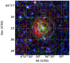
Figure 8: Three-colour image of J0456-6533. red: $0.3\mbox{--}$0.7\text{\,}\mathrm{keV}$$, green: $0.7\mbox{--}$1.1\text{\,}\mathrm{keV}$$ and blue: $1.1\mbox{--}$4.5\text{\,}\mathrm{keV}$$. The inner white circle and the annulus around it mark the two source extraction regions. The green annular region around the SNR shows the background extraction region.

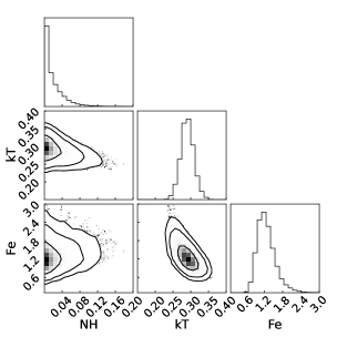
Figure 9: Contour plot for the fitted parameters in the inner region of the remnant. The plotted contours are at $1$,$2$, and $3\sigma$. From the contours, we measure the enhancement of Fe, which is always larger than $0.5\,\mathrm{Z}_{\odot}$, i.e., the average abundance of ISM elements in the LMC.

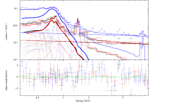
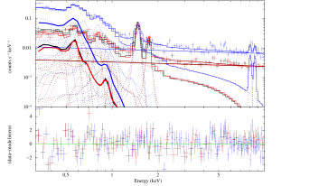
Figure 10: XMM-Newton EPIC spectra of the inner circular region (top) and outer shell (bottom) of SNR J0456–6533. We plot the source spectrum (MOS1: black, MOS2: red, pn: blue) and the best-fit models. The thick solid lines show the contribution of the VNEI source emission component.

8 Conclusions

We investigated the SRG/eROSITA data which provides a complete look at the LMC in the high-energy regime, and we studied the SNR population in the LMC. The large field of view of eROSITA and the full coverage in eRASS:4 allowed us to study the SNR population in the LMC. Furthermore, we used the sensitivity of eROSITA to investigate the X-ray counterpart of the SNR candidates proposed in previous studies and detected at radio and optical wavelengths.

1. Using a $3\sigma$ threshold we were able to confirm two previously known candidates as SNRs: MCSNR J0454–7003 and MCSNR J0539–7001.

2. We performed a Gaussian gradient magnitude filter analysis on the eRASS:4 images of the LMC to detect new SNR candidates. By combining the X-ray data with optical and radio data, we propose 13 sources as new X-ray SNR candidates. Using the HR and the SFH around each source we investigated the origin of the SNR candidate.

3. We propose J0614–7251 as the first X-ray SNR candidate in the outskirts of the LMC. The source presents emission above the $3\sigma$ level with a net counts rate of $0.26\pm 0.01$ photons $\mathrm{s}^{-1}$, resulting in a prominent isolated source. From the SFH we can not rule out a CC origin for this SNR candidate.

4. We use a multi-wavelength analysis to confirm three of the eROSITA candidates as SNRs. This result brings the total number of SNRs in the LMC to 78 and the number of SNR candidates to 46.

5. We have performed a spectral analysis of the newly detected MCSNR J0456–6533 using XMM-Newton data from a follow-up observation of the eROSITA detection. We modelled the source emission with a single absorbed NEI model and investigated different regions of the source. The column density in the LMC is very low $(N_{\text{H}}<0.07\times 10^{22}\,\unit{\per\squared})$ which suggests an un-absorbed source. We do not observe a significant difference in the fitted temperature between the inner part and the outer shell of the remnant. We found an enhancement in Fe abundance in the inner part, which is most likely dominated by ejecta emission and suggests a type Ia SN as the progenitor of MCSNR J0456–6533.

Appendix A Tables

Table 4: Complete catalogue of the known X-ray SNRs in the LMC.

MCSNR	RA [J2000]	DEC [J2000]	Size [$\unit$] (PA [$\deg$])	Rate [counts $\mathrm{s}^{-1}$]	Ref
J0447$-$6918	04:47:12.2	$-$69:19:16	180.9$\times$115.6 (320)	0.03 $\pm$ 0.01	B17
J0448$-$6700	04:48:25.2	$-$67:00:25	321.5	0.21 $\pm$ 0.02	BGS06
J0449$-$6903	04:49:34.0	$-$69:03:34	108.3$\times$103.8 (0)	0.04 $\pm$ 0.01	B17
J0449$-$6920	04:49:20.0	$-$69:20:20	195.6	0.04 $\pm$ 0.01	KPS10
J0450$-$7050	04:50:27.0	$-$70:50:15	383.2	0.28 $\pm$ 0.02	MFT85
J0453$-$6655	04:53:10.2	$-$66:54:52	255.8	0.56 $\pm$ 0.02	SCM94
J0453$-$6829	04:53:37.7	$-$68:29:38	200.6	6.25 $\pm$ 0.06	LHG81
J0454$-$6626	04:54:49.0	$-$66:25:32	150.4	0.25 $\pm$ 0.01	MC73
J0454$-$6713	04:54:27.2	$-$67:13:20	262.0	0.63 $\pm$ 0.02	SCM94
J0454$-$7003	04:54:19.8	$-$70:03:27	75.3$\times$74.2 (80)	$0.04\pm 0.01$	Y20
J0455$-$6839	04:55:29.2	$-$68:39:01	436.6	0.74 $\pm$ 0.03	MC73
J0456$-$6533	04:56:50.7	$-$65:32:44	340.9	0.21 $\pm$ 0.01	TW
J0456$-$6950	04:56:38.0	$-$69:50:55	159.6$\times$129.0 (0)	0.02 $\pm$ 0.01	B17
J0459$-$7008	04:59:51.9	$-$70:07:50	239.4	0.29 $\pm$ 0.02	MC73
J0504$-$6723	05:04:46.1	$-$67:23:59	330.1	0.16 $\pm$ 0.01	HP99
J0505$-$6753	05:05:41.9	$-$67:52:45	134.5	11.14 $\pm$ 0.08	LHG81
J0505$-$6802	05:05:54.7	$-$68:01:50	65.2$\times$53.1 (45)	5.77 $\pm$ 0.05	MC73
J0506$-$6541	05:05:59.8	$-$65:42:37	515.0	0.24 $\pm$ 0.02	KPS10
J0506$-$6815	05:06:07.1	$-$68:15:43	132.5$\times$120.3 (30)	0.11 $\pm$ 0.01	B17
J0506$-$7009	05:06:15.8	$-$70:09:20	97.8$\times$71.8 (140)	0.10 $\pm$ 0.01	TW
J0506$-$7026	05:06:50.0	$-$70:25:53	327.1	0.60 $\pm$ 0.02	Lea17
J0507$-$6847	05:07:33.6	$-$68:47:27	416.6$\times$310.0 (120)	1.41 $\pm$ 0.04	B17
J0508$-$6830	05:08:50.0	$-$68:30:50	205.8	0.06 $\pm$ 0.01	MHK14
J0508$-$6902	05:08:37.0	$-$69:02:54	216.14	0.21 $\pm$ 0.01	BKM14
J0509$-$6731	05:09:30.6	$-$67:31:20	91.42	1.03 $\pm$ 0.02	LHG81
J0509$-$6844	05:08:59.0	$-$68:43:35	144.7	5.22 $\pm$ 0.05	MC73
J0510$-$6708	05:10:11.4	$-$67:08:04	240	0.02 $\pm$ 0.01	B17
J0511$-$6759	05:11:17.4	$-$67:59:10	248.5	0.10 $\pm$ 0.01	MHK14
J0512$-$6707	05:12:27.0	$-$67:07:18	158.6	0.05 $\pm$ 0.01	KSB15b
J0512$-$6716	05:12:24.7	$-$67:16:55	233.8$\times$223.9 (45)	0.20 $\pm$ 0.02	B17
J0513$-$6724	05:13:43.0	$-$67:24:10	78.0$\times$57.4 (0)	0.05 $\pm$ 0.01	Ma19
J0513$-$6912	05:13:10.8	$-$69:12:16	259.4	0.18 $\pm$ 0.01	MFT85
J0514$-$6840	05:14:12.9	$-$68:40:15	289.8	0.18 $\pm$ 0.01	MHK14
J0517$-$6759	05:17:11.7	$-$67:58:50	315.1	0.08 $\pm$ 0.01	MHK14
J0518$-$6939	05:18:41.7	$-$69:39:20	206.9	0.42 $\pm$ 0.02	MC73
J0519$-$6902	05:19:33.3	$-$69:02:21	153.5	3.96 $\pm$ 0.04	LHG81
J0519$-$6926	05:19:44.0	$-$69:26:08	278.9	1.00 $\pm$ 0.02	MFD83
J0521$-$6543	05:21:39.0	$-$65:43:07	394.3	0.06 $\pm$ 0.01	BGS06
J0522$-$6543	05:22:53.5	$-$65:43:09	171.0$\times$159.0 (26)	0.01 $\pm$ 0.01	B23
J0522$-$6740	05:22:33.7	$-$67:41:04	122.1$\times$119.9 (90)	0.12 $\pm$ 0.01	Y20
J0523$-$6753	05:23:05.5	$-$67:53:20	285.7	0.44 $\pm$ 0.02	CMG93
J0524$-$6624	05:24:20.8	$-$66:24:28	255.1	0.02 $\pm$ 0.01	MFT85
J0525$-$6559	05:25:24.1	$-$65:59:26	221.1	11.55 $\pm$ 0.07	MC73
J0525$-$6938	05:25:02.9	$-$69:38:43	219.5	130.79 $\pm$ 0.51	WM66
J0526$-$6605	05:25:59.4	$-$66:05:04	159.1	25.08 $\pm$ 0.11	WM66
J0527$-$6550	05:27:54.0	$-$65:49:38	309.8	0.52 $\pm$ 0.01	LHG81
J0527$-$6714	05:28:07.9	$-$67:13:43	412.83	0.16 $\pm$ 0.02	TM84
J0527$-$6912	05:27:39.7	$-$69:12:20	232.65	0.43 $\pm$ 0.02	MFD84
J0527$-$7104	05:28:01.2	$-$71:04:23	226.8$\times$126.9 (65)	0.18 $\pm$ 0.01	KSP13
J0527$-$7134	05:27:49.9	$-$71:34:08	116.4$\times$107.1 (45)	0.07 $\pm$ 0.01	B17
J0528$-$6727	05:28:05.0	$-$67:27:20	342.3	0.30 $\pm$ 0.01	MHB12
J0529$-$6653	05:29:49.2	$-$66:53:34	211.4	0.41 $\pm$ 0.01	BFC12a
J0529$-$7004	05:29:11.4	$-$70:04:40	157.9$\times$144.7 (0)	0.24 $\pm$ 0.02	Y20
J0530$-$7008	05:30:39.0	$-$70:07:30	349.6	0.78 $\pm$ 0.02	DFB12
J0531$-$7100	05:31:56.0	$-$71:00:19	241.8	1.16 $\pm$ 0.02	MC73

Table 5: Complete catalogue of the known X-ray SNRs in the LMC (continued).

MCSNR	RA [J2000]	DEC [J2000]	Size [$\unit$] (PA [$\deg$])	Rate [counts $\mathrm{s}^{-1}$]	Ref
J0532$-$6732	05:32:14.0	$-$67:32:10	318.6	0.94 $\pm$ 0.02	MFT85
J0533$-$7202	05:33:53.3	$-$72:02:57	261.1	0.26 $\pm$ 0.01	BFC13
J0534$-$6955	05:34:00.4	$-$69:55:03	198.3	2.87 $\pm$ 0.04	LHG81
J0534$-$7033	05:34:14.9	$-$70:33:46	245.7	0.65 $\pm$ 0.02	LHG81
J0535$-$6602	05:35:44.9	$-$66:02:09	187.4	44.01 $\pm$ 0.26	WM66
J0535$-$6916	05:35:27.7	$-$69:16:15	84.4	0.91 $\pm$ 0.02	HISTORICAL
J0535$-$6918	05:35:47.2	$-$69:18:14	131.0	0.30 $\pm$ 0.01	CDS95
J0536$-$6735	05:35:56.2	$-$67:34:07	203.1$\times$108.6 (66)	1.07 $\pm$ 0.02	MFT85
J0536$-$6913	05:36:15.4	$-$69:13:07	108.9	0.20 $\pm$ 0.01	KSB15a
J0536$-$7039	05:36:01.3	$-$70:38:26	270.1	0.63 $\pm$ 0.02	LHG81
J0537$-$6628	05:37:30.9	$-$66:27:52	132.4$\times$90.1 (315)	0.11 $\pm$ 0.01	KPS10
J0537$-$6910	05:37:47.4	$-$69:10:17	156.9	0.69 $\pm$ 0.02	MC73
J0539$-$7001	05:39:35.5	$-$70:01:52	177.9$\times$69.9 (135)	0.42 $\pm$ 0.01	HP99
J0540$-$6920	05:40:10.3	$-$69:19:59	85.6	1.11 $\pm$ 0.02	MC73
J0540$-$6944	05:40:06.1	$-$69:44:00	85.8	0.97 $\pm$ 0.02	CKS97
J0541$-$6659	05:41:49.5	$-$66:58:44	333.3	0.44 $\pm$ 0.02	GSH12
J0542$-$7104	05:42:42.0	$-$71:04:29	104.5$\times$102.6 (0)	0.06 $\pm$ 0.01	Y20
J0543$-$6624	05:43:48.6	$-$66:23:51	334.2	0.15 $\pm$ 0.01	TW
J0543$-$6858	05:43:05.9	$-$68:59:03	338.1	0.99 $\pm$ 0.02	LHG81
J0547$-$6941	05:47:23.2	$-$69:41:23	159.9	0.64 $\pm$ 0.01	MC73
J0547$-$6943	05:46:59.2	$-$69:43:05	133.1$\times$87.93 (35)	0.64 $\pm$ 0.01	MC73
J0547$-$7025	05:47:48.2	$-$70:24:54	204.7	1.17 $\pm$ 0.02	MFD83
J0550$-$6823	05:50:30.9	$-$68:23:43	209.4$\times$167.7 (25)	0.53 $\pm$ 0.03	BFC12b

B17: Bozzetto et al. (2017); B23: Bozzetto et al. (2023); BFC12a: Bozzetto et al. (2012a); BFC12b: Bozzetto et al. (2012b); BFC13: Bozzetto et al. (2013); BGS06: Blair et al. (2006); BKM14: Bozzetto et al. (2014); CDS95: Chu et al. (1995); CKS97: Chu et al. (1997); CMG93: Chu et al. (1993); DFB12: De Horta et al. (2012); GSH12: Grondin et al. (2012); HP99: Haberl & Pietsch (1999a); KPS10: Klimek et al. (2010); KSB15a: Kavanagh et al. (2015a); KSB15b: Kavanagh et al. (2015b); KSP13: Kavanagh et al. (2013); Lea17: Leahy (2017); LHG81: Long et al. (1981); Ma19: Maitra et al. (2019); MC73: Mathewson & Clarke (1973); MFD83: Mathewson et al. (1983); MFD84: Mathewson et al. (1984); MFT85: Mathewson et al. (1985); MHB12: Maggi et al. (2012); MHK14: Maggi et al. (2014); SCM94: Smith et al. (1994); TM84: Turtle & Mills (1984); TW: this work; WM66: Westerlund & Mathewson (1966); Y20: Yew et al. (2021).

Table 6: X-ray SNRs in the LMC detected for the first time by eROSITA and confirmed as SNRs in this work.

MCSNR	RA [J2000]	DEC [J2000]	Size [$\unit$] (PA [$\deg$])	Rate [counts $\mathrm{s}^{-1}$]	HR1	HR2	HR3
J0456$-$6533	04:56:50.7	$-$65:32:44	340.9	$0.21\pm 0.01$	$-0.27\pm 0.04$	-	-
J0506$-$7009	05:06:15.8	$-$70:09:20	97.8$\times$71.8 (140)	$0.10\pm 0.01$	$0.72\pm 0.08$	$-0.68\pm 0.08$	$-0.41\pm 0.24$
J0543$-$6624	05:43:48.6	$-$66:23:51	334.2	$0.14\pm 0.01$	$-0.49\pm 0.03$	$-0.72\pm 0.08$	-

Table 7: SNR candidates proposed in previous works and confirmed as SNRs in this work with eROSITA.

MCSNR	RA [J2000]	DEC [J2000]	Size [$\unit$] (PA [$\deg$])	Rate [counts $\mathrm{s}^{-1}$]	HR1	HR2	HR3	Ref
J0454$-$7003	04:54:19.8	$-$70:03:27	75.3$\times$74.2 (80)	$0.04\pm 0.01$	$-0.69\pm 0.12$	$-0.61\pm 0.39$	-	Y21
J0539$-$7001	05:39:35.5	$-$70:01:52	177.9$\times$69.9 (135)	$0.42\pm 0.01$	$0.60\pm 0.03$	$-0.77\pm 0.03$	$-0.62\pm 0.11$	HP99

HP99: Haberl & Pietsch (1999a), Y21: Yew et al. (2021).

Table 8: New X-ray SNR candidates in the LMC found with eROSITA for the first time.

4eRASSU	RA [J2000]	DEC [J2000]	Size [$\unit$] (PA [$\deg$])	Rate [counts $\mathrm{s}^{-1}$]	HR1	HR2	HR3
J045145.7$-$671724	04:51:45.7	$-$67:17:24	292.5$\times$170.8 (60)	$0.22\pm 0.02$	$-0.01\pm 0.05$	$-0.61\pm 0.09$	$-0.03\pm 0.23$
J045625.5$-$683052	04:56:25.5	$-$68:30:52	160.2	$0.03\pm 0.01$	$0.81\pm 0.18$	$-0.79\pm 0.20$	$<0.01$
J050750.8$-$714241	05:07:50.8	$-$71:42:41	146.3$\times$114.1 (359)	$0.07\pm 0.01$	$0.63\pm 0.12$	-	-
J051028.3$-$685329	05:10:28.3	$-$68:53:29	224.4	$0.10\pm 0.01$	$-0.21\pm 0.09$	$-0.22\pm 0.11$	$-0.53\pm 0.21$
J052136.6$-$670741	05:21:36.6	$-$67:07:41	398.1	$0.09\pm 0.01$	$-0.28\pm 0.09$	-	-
J052126.5$-$685245	05:21:26.5	$-$68:52:45	311.3	$0.02\pm 0.01$	-	-	-
J052148.7$-$693649	05:21:48.7	$-$69:36:49	314.1	$0.09\pm 0.02$	$0.73\pm 0.11$	-	-
J052330.7$-$680400	05:23:30.7	$-$68:04:00	232.8	$0.03\pm 0.01$	$0.71\pm 0.16$	$-0.57\pm 0.14$	-
J052502.7$-$662125	05:25:02.7	$-$66:21:25	308.1	$0.11\pm 0.01$	$0.29\pm 0.05$	$-0.75\pm 0.07$	-
J052849.7$-$671913	05:28:49.7	$-$67:19:13	229.3	$0.04\pm 0.01$	$-0.03\pm 0.15$	$-0.30\pm 0.17$	-
J053224.5$-$655411	05:32:24.5	$-$65:54:11	166.6	$0.07\pm 0.01$	$0.22\pm 0.06$	$-0.39\pm 0.06$	-
J054949.7$-$700145	05:49:49.7	$-$70:01:45	158.5$\times$101.9 (160)	$0.06\pm 0.01$	$0.75\pm 0.07$	$-0.86\pm 0.09$	-
J061438.1$-$725112	06:14:38.1	$-$72:51:12	214.4	$0.26\pm 0.01$	$-0.29\pm 0.03$	$-0.70\pm 0.06$	$-0.85\pm 0.28$

Table 9: X-rays SNRs confirmed in Maitra et al. (2019), Yew et al. (2021), Kavanagh et al. (2022), Maitra et al. (2021), Sasaki et al. (2022), and Bozzetto et al. (2023).

MCSNR	RA [J2000]	DEC [J2000]	Size [$\unit$] (PA [$\deg$])	Rate [counts $\mathrm{s}^{-1}$]	HR1	HR2	HR3	Conf
J0447$-$6918	04:47:12.2	$-$69:19:16	180.9$\times$115.6 (320)	$0.03\pm 0.01$	$0.14\pm 0.16$	$-0.68\pm 0.27$	-	K22
J0449$-$6903	04:49:34.0	$-$69:03:34	108.3$\times$103.8(0)	$0.04\pm 0.01$	$-0.06\pm 0.20$	$0.13\pm 0.20$	$-0.42\pm 0.30$	K22
J0456$-$6950	04:56:38.0	$-$69:50:55	159.6$\times$129.0 (0)	$0.02\pm 0.01$	-	-	-	K22
J0504$-$6723	05:04:46.1	$-$67:23:59	330.1	$0.16\pm 0.01$	$0.57\pm 0.05$	$-0.90\pm 0.07$	-	K22
J0506$-$6815	05:06:07.1	$-$68:15:43	132.5$\times$120.3 (30)	$0.11\pm 0.01$	$-0.04\pm 0.08$	$-0.15\pm 0.09$	-	B23
J0507$-$6847	05:07:33.6	$-$68:47:27	416.6$\times$310.0 (120)	$1.40\pm 0.04$	$-0.16\pm 0.02$	$-0.65\pm 0.03$	$-0.65\pm 0.11$	Ma21
J0510$-$6708	05:10:11.4	$-$67:08:04	240.0	$0.02\pm 0.01$	$0.23\pm 0.24$	$-0.50\pm 0.32$	$-0.33\pm 0.98$	K22
J0512$-$6716	05:12:24.7	$-$67:16:55	233.8$\times$223.9 (45)	$0.20\pm 0.02$	$-0.37\pm 0.05$	$-0.74\pm 0.11$	-	K22
J0513$-$6724	05:13:43.0	$-$67:24:10	78.0$\times$57.0 (0)	$0.05\pm 0.01$	$-0.01\pm 0.01$	$-0.22\pm 0.01$	$-0.70\pm 0.21$	Ma19
J0522$-$6543	05:22:53.5	$-$65:43:09	171.0$\times$159.0	$0.01\pm 0.01$	-	-	-	B23
J0522$-$6740	05:22:33.7	$-$67:41:04	122.1$\times$119.9	$0.12\pm 0.01$	$-0.03\pm 0.05$	-	-	Y21
J0527$-$7134	05:27:49.9	$-$71:34:08	116.4$\times$107.1 (45)	$0.07\pm 0.01$	$0.41\pm 0.05$	$-0.85\pm 0.07$	-	K22
J0529$-$7004	05:29:11.4	$-$70:04:40	157.9$\times$144.7 (0)	$0.24\pm 0.02$	$-0.05\pm 0.06$	$-0.81\pm 0.10$	$<0.01$	Sa22
J0542$-$7104	05:42:42.0	$-$71:04:29	104.5$\times$102.6 (0)	$0.06\pm 0.01$	$0.76\pm 0.08$	$-0.73\pm 0.09$	-	Y21

Ma19: Maitra et al. (2019); Y21: Yew et al. (2021); Ma21: Maitra et al. (2021); K22: Kavanagh et al. (2022); Sa22: Sasaki et al. (2022); B23: Bozzetto et al. (2023) .

Table 10: X-ray SNR candidates in the LMC proposed in previous works which do not have a 3$\sigma$ eROSITA counterpart.

ID	RA [J2000]	DEC [J2000]	Size [$\unit$] (PA [$\deg$])	Rate [counts $\mathrm{s}^{-1}$]	HR1	HR2	HR3	Ref
J0444$-$6758	04:44:27.8	$-$67:58:13	77.54 $\times$ 54.6(80)	$0.01\pm 0.01$	-	-	-	Y21
J0450$-$6818	04:50:12.4	$-$68:18:05	454.0$\times$366.0 (105)	$0.15\pm 0.03$	$-0.068\pm 0.12$	$-0.54\pm 0.22$	$0.34\pm 0.32$	Y21
J0451$-$6906	04:51:38.9	$-$69:06:26	299.0$\times$194.0 (345)	$0.09\pm 0.02$	$0.06\pm 0.12$	$-0.84\pm 0.24$	$0.66\pm 0.49$	B23
J0451$-$6951	04:51:52.7	$-$69:51:41	170.0$\times$168.0 (0)	$0.04\pm 0.01$	$-0.44\pm 0.19$	-	-	B23
J0452$-$6638	04:52:42.2	$-$66:38:43	277.0$\times$ 196.0 (0)	$0.04\pm 0.02$	$-0.08\pm 0.12$	-	-	B23
J0455$-$6830	04:55:36.8	$-$68:30:35	80.0$\times$78.0(170)	$<0.001$	-	-	-	Y21
J0457$-$6739	04:57:33.0	$-$67:39:05	300.0	$<0.001$	-	-	-	B17
J0457$-$6823	04:57:33.6	$-$68:23:39	196.0$\times$115 (330)	$0.07\pm 0.01$	$-0.29\pm 0.13$	$-0.38\pm 0.22$	$0.14\pm 0.32$	B23
J0457$-$6923	04:57:07.8	$-$69:23:58	122.0$\times$100.9 (90)	$0.09\pm 0.01$	$0.16\pm 0.10$	$-0.62\pm 0.14$	$0.24\pm 0.25$	B17
J0459$-$6757	04:59:55.0	$-$67:57:01	131.0$\times$114.0 (357)	$0.02\pm 0.01$	$0.10\pm 0.23$	$-0.25\pm 0.25$	-	B23
J0459$-$7008b	04:59:38.7	$-$70:08:37	112.6$\times$95.9(150)	$0.21\pm 0.01$	$-0.27\pm 0.05$	$-0.79\pm 0.09$	-	B23
J0500$-$6512	05:00:53.2	$-$65:11:46	238.8$\times$174.3 (80)	$0.05\pm 0.01$	$0.77\pm 0.12$	-	-	Y21
J0502$-$6739	05:02:02.5	$-$67:39:31	190.0$\times$168.0 (60)	$0.02\pm 0.01$	$0.23\pm 0.28$	$-0.29\pm 0.29$	-	Y21
J0504$-$6901	05:04:04.8	$-$69:01:12	259.0$\times$246.0 (22)	$0.10\pm 0.02$	$-0.41\pm 0.10$	-	-	B23
J0506$-$6509	05:06:49.1	$-$65:09:19	192.5$\times$184.1 (170)	$0.013\pm 0.009$	$-0.23\pm 0.32$	$-0.46\pm 0.61$	-	Y21
J0507$-$7110	05:07:35.3	$-$71:10:15	221.3$\times$219.0 (0)	$0.08\pm 0.02$	$0.26\pm 0.12$	$-0.90\pm 0.21$	$0.64\pm 0.74$	B17
J0508$-$6928	05:08:46.5	$-$69:28:16	660.0	$<0.001$	-	-	-	Y21
J0509$-$6402	05:09:15.5	$-$64:02:07	164.0$\times$121.0 (50)	$0.04\pm 0.001$	$0.32\pm 0.12$	$-0.50\pm 0.14$	-	Y21
J0513$-$6731	05:13:26.9	$-$-67:31:53	150$\times$105 (60)	$0.03\pm 0.01$	$-0.50\pm 0.24$	$-0.65\pm 0.65$	$0.58\pm 0.75$	B17
J0517$-$6757	05:17:53.6	$-$67:57:25	86.9$\times$85.2 (130)	$<0.001$	-	-	-	Y21
J0528$-$7018	05:28:46.0	$-$70:17:57	278.7$\times$263.4 (140)	$0.17\pm 0.03$	$-0.48\pm 0.09$	$-0.95\pm 0.29$	-	Y21
J0534$-$6700	05:34:42.4	$-$66:59:55	90.3$\times$75.5 (0)	$0.023\pm 0.004$	$-0.52\pm 0.14$	$-0.45\pm 0.30$	-	B23
J0534$-$6720	05:34:04.9	$-$67:20:51	163.3$\times$162.3 (0)	$0.22\pm 0.01$	$-0.51\pm 0.038$	$-0.76\pm 0.10$	-	B23
J0538$-$6921	05:38:14.7	$-$69:21:24	166.1$\times$160.0 (0)	$0.46\pm 0.02$	$0.58\pm 0.04$	$-0.44\pm 0.03$	-	B17
J0538$-$7004	05:38:44.9	$-$70:04:24	160	$0.004\pm 0.004$	$-0.25\pm 0.33$	-	-	Y21
J0542$-$6852	05:41:59.3	$-$68:52:01	181.51$\times$174.9 (343)	$0.32\pm 0.01$	$0.21\pm 0.03$	$-0.63\pm 0.04$	$-0.69\pm 0.15$	B23
J0543$-$6906	05:43:27.0	$-$69:07:21	438.5	$0.14\pm 0.03$	$-0.08\pm 0.18$	$0.07\pm 0.13$	$-0.59\pm 0.18$	B23
J0543$-$6923	05:43:16.5	$-$69:23:27	288.0$\times$213.0 (0)	$0.13\pm 0.02$	$-0.25\pm 0.19$	$0.24\pm 0.14$	$-0.31\pm 0.14$	B23
J0543$-$6928	05:43:06.3	$-$69:28:42	145.0$\times$89.1 (35)	$0.02\pm 0.01$	-	$0.12\pm 0.19$	-	B23
J0548$-$6941	05:48:49.2	$-$69:41:22	156.0$\times$95.0 (150)	$<0.001$	-	-	-	Y21
J0549$-$6618	05:49:30.4	$-$66:17:37	64.9$\times$57.2 (45)	$<0.001$	-	-	-	Y21
J0549$-$6633	05:49:25.6	$-$66:33:46	175.5$\times$124.3 (45)	$0.047\pm 0.004$	-	-	-	Y21
J0624$-$6948	06:24:13.5	$-$69:48:31	272.2	$0.05\pm 0.001$	$-0.40\pm 0.11$	$0.29\pm 0.11$	-	F22

B17: Bozzetto et al. (2017); B23: Bozzetto et al. (2023); F22: Filipović et al. (2022) Y21: Yew et al. (2021).

Appendix B MCSNR and candidate Images

Appendix A SNR candidates detected with eROSITA

ı/ȷin J0451-6717/4eRASSU J045145.7–671724,J0456-6830/4eRASSU J045625.5–683052,J0507-7143/4eRASSU J050750.8–714241,J0510-6853/4eRASSU J051028.3–685329,J0521-6707/4eRASSU J052136.6–670741,J0521-6853/4eRASSU J052126.5–685245,J0521-6936/4eRASSU J052148.7–693649,J0523-6804/4eRASSU J052330.7–680400,J0525-6621/4eRASSU J052502.7–662125

(a) ȷ

Figure 11: For each source we show the eROSITA count rate three-colour image (left) with red: $0.2\mbox{--}$0.7\text{\,}\mathrm{keV}$$, green: $0.7\mbox{--}$1.1\text{\,}\mathrm{keV}$$, and blue: $1.1\mbox{--}$5.0\text{\,}\mathrm{keV}$$, the GGM filter image (see Sect. 3.3) applied to the eROSITA count rate (middle left), the MCELS survey three-colour image (middle right) with red: H$\alpha$, green: [S II], and blue: [O III], and the ASKAP radio continuum (right) in the upper panel. The cyan (red) contours in the eROSITA three-colour image show the detection at 1 and $2\sigma\ (3\sigma)$ over the background in the energy band $0.2\mbox{--}$1.1\text{\,}\mathrm{keV}$$. The contours in the optical image represent [S II]/H$\alpha>0.67$. The contours in the radio image show the non-thermal emission calculated as described in Sect. 4.2. In the lower panel we show the SFH as measured in Mazzi et al. (2021).

ı/ȷin J0528-6719/4eRASSUJ052849.7–671913,J0532-6554/4eRASSU J053224.5–655411,J0549-7001/4eRASSU J054949.7–700145

(a) ȷ

Figure 12: For each source we show the eROSITA count rate three-colour image (left) with red: $0.2\mbox{--}$0.7\text{\,}\mathrm{keV}$$, green: $0.7\mbox{--}$1.1\text{\,}\mathrm{keV}$$, and blue: $1.1\mbox{--}$5.0\text{\,}\mathrm{keV}$$, the GGM filter image (see Sect. 3.3) applied to the eROSITA count rate (middle left), the MCELS survey three-colour image (middle right) with red: H$\alpha$, green: [S II], and blue: [O III], and the ASKAP radio continuum (right) in the upper panel. The cyan (red) contours in the eROSITA three-colour image show the detection at 1 and $2\sigma\ (3\sigma)$ over the background in the energy band $0.2\mbox{--}$1.1\text{\,}\mathrm{keV}$$. The contours in the optical image represent [S II]/H$\alpha>0.67$. The contours in the radio image show the non-thermal emission calculated as described in Sect. 4.2. In the lower panel we show the SFH as measured in Mazzi et al. (2021).

Appendix B Previous candidate from ROSAT confirmed with eROSITA

ı/ȷin J0539-7001/MCSNR J0539–7001,J0454-7003/MCSNR J0454–7003

(a) ȷ

Figure 13: From left to right we show the eROSITA count rate three-colour image where red: $0.2\mbox{--}$0.7\text{\,}\mathrm{keV}$$, green: $0.7\mbox{--}$1.1\text{\,}\mathrm{keV}$$, and blue: $1.1\mbox{--}$5.0\text{\,}\mathrm{keV}$$. The cyan (red) contours show the detection at 1 and $2\sigma\ (3\sigma)$ over the background in the energy band $0.2\mbox{--}$1.1\text{\,}\mathrm{keV}$$. The second image shows the GGM filter applied to the eROSITA count rates (GGM filter described in Sect. 3.3). The third image shows the MCELS survey three-colour image where red: H$\alpha$, green: [S II], and blue: [O III]. The contours in the optical image represent [S II]/H$\alpha>0.67$. The last image shows the ASKAP radio continuum. The contours in the radio image show the non-thermal emission calculated as described in Sect. 4.2.

Appendix C Previous candidates which remain candidates

ıin J0444-6758,J0450-6818,J0451-6906

(a) ı

Figure 14: From left to right we show the eROSITA count rate three-colour image where red: $0.2\mbox{--}$0.7\text{\,}\mathrm{keV}$$, green: $0.7\mbox{--}$1.1\text{\,}\mathrm{keV}$$, and blue: $1.1\mbox{--}$5.0\text{\,}\mathrm{keV}$$. The cyan (red) contours show the detection at 1 and $2\sigma\ (3\sigma)$ over the background in the energy band $0.2\mbox{--}$1.1\text{\,}\mathrm{keV}$$. The second image shows the GGM filter applied to the eROSITA count rates (GGM filter described in section 3.3). The third image shows the MCELS survey three-colour image where red: H$\alpha$, green: [S II], and blue: [O III]. The contours in the optical image represent [S II]/H$\alpha>0.67$. The last image shows the ASKAP radio continuum. The contours in the radio image show the non-thermal emission calculated as described in section 4.2.

ıin J0451-6951,J0452-6638,J0455-6830,J0457-6739,J0457-6823,J0457-6923,J0459-6757,J0459-7008b,J0500-6512,J0502-6739,J0504-6901,J0506-6509,J0507-7110,J0508-6928,J0509-6402,J0513-6731,J0517-6757,J0528-7018

(a) ı

Figure 15: From left to right we show the eROSITA count rate three-colour image where red: $0.2\mbox{--}$0.7\text{\,}\mathrm{keV}$$, green: $0.7\mbox{--}$1.1\text{\,}\mathrm{keV}$$, and blue: $1.1\mbox{--}$5.0\text{\,}\mathrm{keV}$$. The cyan (red) contours show the detection at 1 and $2\sigma\ (3\sigma)$ over the background in the energy band $0.2\mbox{--}$1.1\text{\,}\mathrm{keV}$$. The second image shows the GGM filter applied to the eROSITA count rates (GGM filter described in section 3.3). The third image shows the MCELS survey three-colour image where red: H$\alpha$, green: [S II], and blue: [O III]. The contours in the optical image represent [S II]/H$\alpha>0.67$. The last image shows the ASKAP radio continuum. The contours in the radio image show the non-thermal emission calculated as described in section 4.2.

ıin J0534-6700,J0534-6720,J0538-6921,J0538-7004,J0542-6852,J0543-6906,J0543-6923,J0543-6928,J0548-6941,J0549-6618,J0549-6633,J0624-6948

(a) ı

Figure 16: From left to right we show the eROSITA count rate three-colour image where red: $0.2\mbox{--}$0.7\text{\,}\mathrm{keV}$$, green: $0.7\mbox{--}$1.1\text{\,}\mathrm{keV}$$, and blue: $1.1\mbox{--}$5.0\text{\,}\mathrm{keV}$$. The cyan (red) contours show the detection at 1 and $2\sigma\ (3\sigma)$ over the background in the energy band $0.2\mbox{--}$1.1\text{\,}\mathrm{keV}$$. The second image shows the GGM filter applied to the eROSITA count rates (GGM filter described in section 3.3). The third image shows the MCELS survey three-colour image where red: H$\alpha$, green: [S II], and blue: [O III]. The contours in the optical image represent [S II]/H$\alpha>0.67$. The last image shows the ASKAP radio continuum. The contours in the radio image show the non-thermal emission calculated as described in section 4.2.

Appendix D Known SNRs not included in Maggi et al. (2016) and detected with eROSITA

ı/ȷin J0447-6918/MCSNR J0447-6918,J0449-6903/MCSNR J0449-6903,J0456-6950/MCSNR J0456-6950,J0504-6723/MCSNR J0504-6723,J0506-6815/MCSNR J0506-6815,J0507-6847/MCSNR J0507-6847,J0510-6708/MCSNR J0510-6708,J0512-6716/MCSNR J0512-6716,J0513-6724/MCSNR J0513-6724,J0522-6543/MCSNR J0522-6543,J0522-6740/MCSNR J0522-6740,J0527-7134/MCSNR J0527-7134,J0529-7004/MCSNR J0529-7004,J0542-7104/MCSNR J0542-7104

(a) ȷ

Figure 17: From left to right we show the eROSITA count rate three-colour image where red: $0.2\mbox{--}$0.7\text{\,}\mathrm{keV}$$, green: $0.7\mbox{--}$1.1\text{\,}\mathrm{keV}$$, and blue: $1.1\mbox{--}$5.0\text{\,}\mathrm{keV}$$. The cyan (red) contours show the detection at 1 and $2\sigma\ (3\sigma)$ over the background in the energy band $0.2\mbox{--}$1.1\text{\,}\mathrm{keV}$$. The second image shows the GGM filter applied to the eROSITA count rates (GGM filter described in section 3.3). The third image shows the MCELS survey three-colour image where red: H$\alpha$, green: [S II], and blue: [O III]. The contours in the optical image represent [S II]/H$\alpha>0.67$. The last image shows the ASKAP radio continuum. The contours in the radio image show the non-thermal emission calculated as described in section 4.2.