Isolated and group environment dependence of stellar mass and different star formation rates

Abstract

In this study, we explored the impact of isolated and group environments on stellar mass, star formation rate (SFR), and specific star formation rate (SSFR, i.e., the rate of star formation per unit stellar mass) using the galaxy dataset from the Sloan Digital Sky Survey Data Release 12 (SDSS DR12) for $z\lesssim 0.2$. To mitigate the Malmquist bias, we partitioned the entire dataset into fifteen subsamples with a redshift bin size of $\Delta z=0.01$ and examined the environmental dependencies of these properties within each redshift bin. A strong correlation between environment, stellar mass, SFR, and SSFR was observed across nearly all redshift bins. In the lower redshift bins $(z<0.1)$, the proportion of galaxies within the isolated environment exceeded that within the group environment. On the other hand, in the higher redshift bins $(z\geq 0.12)$, the isolated environment’s galaxy fraction is found to be lower than that of the group environment. For the intermediate redshift bins $(0.1\leq z<0.12)$, an approximately equal proportion of galaxies is observed in both isolated and group environments.

I Introduction

For a long time, it has been established that galaxy formation and evolution are influenced by both internal physics as well as external surroundings. Mechanisms driving internal physics such as halting star formation in galaxies through processes like heating, expulsion, and gas consumption include feedback from active galactic nuclei and supernovae [5]. Beyond internal physics, the external environment in which galaxies exist is anticipated to be another important factor impacting galaxy evolution. Environments with higher density may elevate the merger rates, potentially triggering a rapid quenching process and inducing changes in the shape and star formation rate (SFR) of galaxies on a condensed timescale [6]. In most studies, the environment has been characterized by the surface number density $n$ of galaxies within the closest neighbours, falling within the range of $3\leq n\leq 10$ [15, 27, 24, 26]. As emphasized by Ref. [14], the utilization of nearest neighbour densities is widespread in describing the local galaxy environment. The optimal choice for the number of neighbours to consider remains a topic of discussion and relies on the characteristics of the sample and the specific survey [15, 29, 27, 24, 26].

The research conducted by Ref. [8] revealed a notable shift of almost a factor of two in the stellar mass distribution of galaxies towards higher masses when comparing low- and high-density regions. Furthermore, the investigation carried out by Ref. [20] indicated that high-density environments predominantly have massive galaxies, in contrast to low-density environments. Additionally, Ref. [9] demonstrated that high-mass galaxies exhibit a preference for the densest regions of the Universe, while low-mass galaxies tend to be situated preferentially in low-density regions.

The study by Ref. [21] demonstrated a robust correlation between the SFRs of galaxies and their local (projected) galaxy densities. Galaxies situated in dense environments exhibit suppressed SFRs [7, 21, 28, 23]. According to Ref. [7], observing low SFRs extending well beyond the virialized cluster suggests that severe physical processes, such as ram pressure stripping of disk gas, may not be the dominant factor. In their investigation, Ref. [16] explored the relationship between the star formation and the environment at both $z\sim 0.1$ and $1$. They reported that in the local Universe, star formation is contingent on the environment, with galaxies in regions of higher over-density generally exhibiting lower SFRs compared to their counterparts in lower-density regions. However, Ref. [22] presented contrasting findings in their study, revealing a reversal of the specific star formation-density relation at $z\sim 1$. The average SFR of individual galaxies increased with local galaxy density when the Universe was less than half of its present age. Ref. [23] extended this exploration to $z\sim 0.8$ and observed a strong decrease in both the SFR and the specific star formation rate (SSFR, i.e., star formation rate per unit stellar mass) with increasing local density, resembling the relation at $z\sim 0$.

In a study focusing on a carefully selected sample of the compact group (CG) of galaxies, Ref. [25] noted significant differences in the SFRs of star-forming galaxies between the isolated and embedded systems. Galaxies in isolated systems exhibited a notable increase in SFR relative to a control sample matched in mass and redshift. Such a trend is not observed in embedded systems. Galaxies in isolated systems displayed a median SFR enhancement at a fixed stellar mass of $+0.07\pm 0.03$ dex.

Emphasizing the importance of a comprehensive approach, it is crucial to recognize that exploring a specific issue may require the use of diverse samples or methodologies to attain more information about it. In line with this perspective, the principal objective of this study is to introduce a novel approach for examining stellar mass, SFR, and SSFR within both isolated and group environments of galaxies. For this purpose, we use the Sloan Digital Sky Survey Data Release 12 (SDSS DR12) for $z\leq 0.2$.

Our paper is organized as follows: In Section II we present the survey from which the data of the galaxy samples are taken. The method of analysis of these data samples is also discussed in this section. Section III is used to present the results and their discussion. We conclude the study in Section IV. Throughout this paper, we consider the cosmological parameters provided in Ref. [19]: the Hubble constant $H_{0}=67.8$ km s^-1 Mpc^-1, the matter density $\Omega_{m}=0.308$, and the dark energy density $\Omega_{\Lambda}=0.692$.

II Data and Analysis

As mentioned in the previous section, this study relies on catalogue data extracted from Sloan Digital Sky Survey Data Release 12 (SDSS DR12) , commonly known as the Legacy Survey [10, 11]. It’s important to note that the galaxy data in SDSS DR16 and DR17, which constitute the final data releases of the SDSS IV, remains virtually unchanged compared to DR12 within the Legacy Survey area [12]. Specifically, we utilize the value-added catalogue of galaxies, groups, and clusters provided by Ref. [13]. The galaxy sample utilized in Ref. [13] is volume-limited and contains $584,449$ galaxies with spectroscopic redshifts up to $z=0.2$, all of which are brighter than the Petrosian r-band magnitude of $17.77$. Additionally, the catalogue includes $88,662$ galaxy groups, each consisting of a minimum of two members. These groups were compiled using a modified friend-of-friend (FoF) method with a variable linking length. The essence of this approach lies in the division of the sample into distinct systems through an objective and automated process. The method involves creating spheres with a linking length ($R$) around each sample point, specifically galaxies in this context To adjust the linking length based on distance, the procedures outlined in Ref. [33, 13] was applied. The relationship between the linking length and the redshift is represented by an arctangent law as given by

$$R_{LL}(z)=R_{LL,0}\left[1+a\arctan\left(\frac{z}{z_{\star}}\right)\right],$$ (1)

where $R_{LL}(z)$ is the linking length used to create a sphere at a specific redshift, $R_{LL,0}$ is the linking length at $z=0$, $a$ and ${z_{\star}}$ are free parameters. The values of $R_{LL,0}=0.34$ Mpc, $a=1.4$ and ${z_{\star}}=0.09$ are obtained by fitting Equation (1) to the linking length scaling relation. If there are other galaxies within the sphere, they are considered as the parts of the same system and referred to as “friends”. Subsequently, additional spheres are drawn around these newly identified neighbours, and the process continues with the principle that “any friend of my friend is my friend”. This iterative procedure persists until no new neighbours or “friends” can be added. At that point, the process concludes, and a system is defined. Two galaxy clusters are said to be interacting if the distance between their centers (in comoving coordinates) is less than the sum of their radii. Consequently, each system comprises either a solitary, isolated galaxy or a group of galaxies that share at least one neighbour within a distance not exceeding $R$. For comprehensive details regarding the compilation of the galaxy samples, refer to Ref. [13].

The data on stellar mass, SFR, and SSFR were derived from the spectroscopic catalogues of the SDSS. The analysis utilized the spectra processed by the Max Planck Institute for Astrophysics and Johns Hopkins University (MPA-JHU). The MPA-JHU employs sophisticated stellar population synthesis models to precisely fit and remove the stellar continuum, yielding a collection of emission-line measurements for the galaxy spectra. This methodology has been applied to earlier releases of SDSS data, and the obtained measurements have been utilized in diverse scientific investigations [17, 8, 31]. The set of line measurements is commonly referred to as the MPA-JHU measurements, named after the Max Planck Institute for Astrophysics and Johns Hopkins University, where the technique was developed. These measurements were provided for all objects identified as galaxies by SDSS software, idlspec2d [32]. This dataset was chosen for its photometric completeness, uniform spectral calibration, broad redshift coverage ($0.02\leq z\leq 0.6$), and a diverse range of emission line properties associated with galaxy formation and evolution, including SFRs, stellar masses (M$\star$), and SSFRs, following the methodologies outlined in Ref. [17, 8, 31].

The determination of stellar masses in the MPA-JHU relies on the Bayesian approach and model grids provided by Ref. [8]. Spectra and photometry are used in conjunction, with a minor correction made for the contribution of nebular emission. For the SDSS spectroscopic fiber aperture, stellar mass is computed using fiber magnitudes, while the overall stellar mass is calculated using model magnitudes. The stellar mass output is represented by probability distribution functions at the median for $2.5\%,16\%,84\%,$ and $97.5\%$ values. Regarding SFR, as detailed in Ref. [17], they are computed within the galaxy fiber aperture using nebular emission lines. For regions outside the fiber, SFRs are estimated using galaxy photometry data obtained from Ref. [18]. In cases of AGNs and galaxies with weak emission lines, SFRs are estimated solely from photometry. The results for both fiber SFR and total SFR include values at the median of $2.5\%,16\%,84\%,$ and $97.5\%$ of the probability distribution functions. Our study utilizes the median estimate which was used to plot the Figures 1, 2, 3, 4, 5 and 6 for the analysis.

The final dataset comprises a total of $571,459$ galaxies, obtained through a $1$ arcsec sky cross-correlation between the value-added catalogue data of SDSS DR12 by Ref. [13] and MPA-JHU. The galaxies with Group Id $=0$ are termed isolated, while the galaxies with Group Id $\neq 0$ are termed groups. Isolated galaxies represent a population of galaxies with minimized environmental evolutionary effects while Group galaxies represent a population of galaxies with high environmental evolutionary effects. In the final dataset, $294,027\,(51\%)$ isolated galaxies and $277,432\,(49\%)$ group galaxies were obtained. It’s also important to address the potential bias introduced by the Malmquist effect, wherein there is a tendency for observers to perceive an increase in averaged luminosity with distance due to the non-detection of less luminous objects at larger distances [30]. This bias can significantly impact statistical results. To mitigate the Malmquist effect, the entire main galaxy sample was divided into subsamples with a redshift binning size of $\Delta z=0.01$ as shown in Table 1. This approach ensures that the radial selection function is approximately uniform within each bin, minimizing variations in the space density of galaxies with radial distance and decreasing the impact of the Malmquist bias.

           

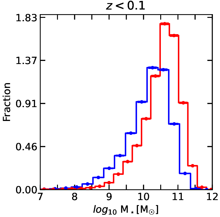
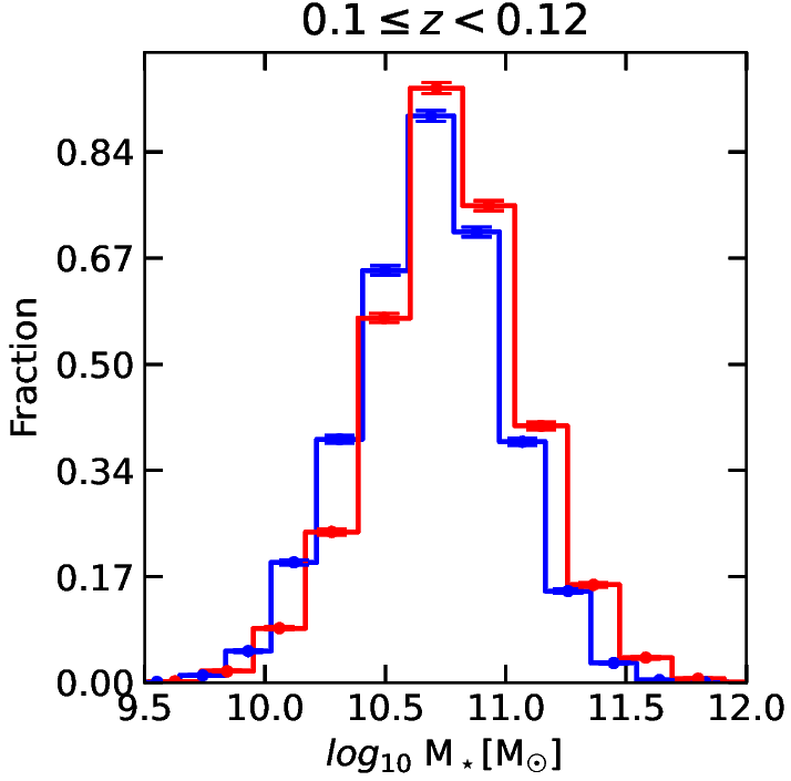
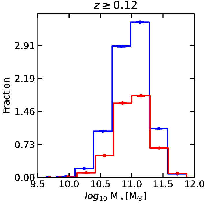
Figure 1: Stellar mass distributions for isolated (blue solid line) galaxies and group galaxies (red solid line). The error bars are 1 $\sigma$ Poissonian errors.

           

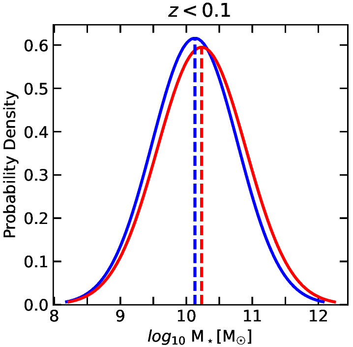
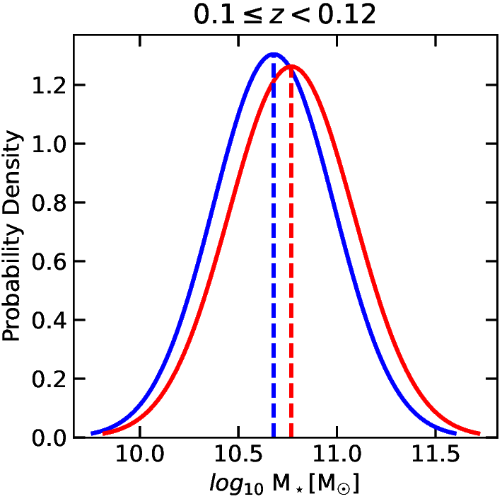
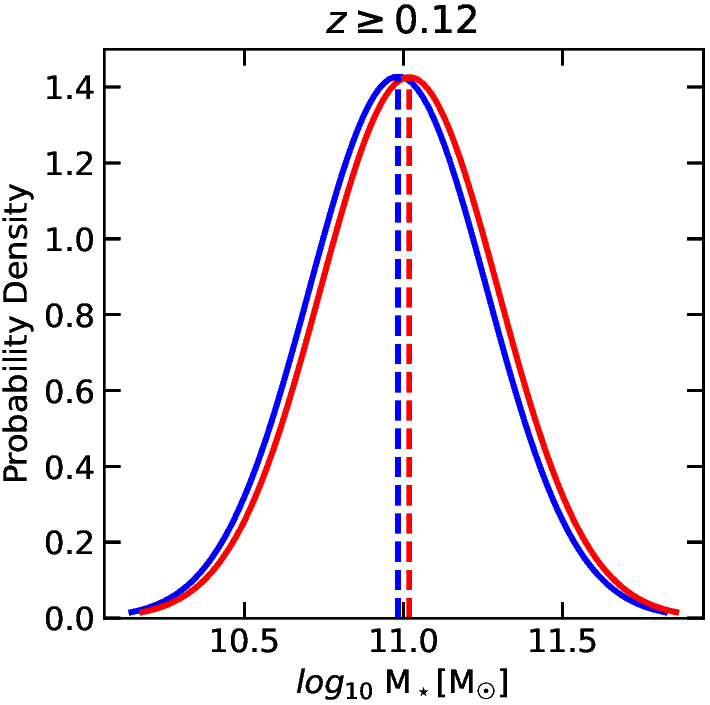
Figure 2: Stellar mass distribution curves as obtained from the Gaussian fitting for isolated (blue solid curve) and group galaxies (red solid curve). Blue and red dotted lines show the position of the median of distributions for isolated and group galaxies respectively.

III Results and Discussion

As already mentioned, the SSFR is defined as the SFR per unit stellar mass, and these quantities were derived by the MPA-JHU group. Figure 1 shows the general distribution of stellar masses within the redshift ranges $z<0.1$, $0.1\leq z<0.12$, and $z\geq 0.12$ in both isolated and group environments. Figure 2 illustrates the corresponding Gaussian distributions of stellar masses for these redshift ranges and both environments. As depicted in Figure 2 and columns (2), (3) of Table 1, high-mass galaxies are consistently found in group environments across all redshift bins, while low-mass galaxies tend to preferentially inhabit in isolated environments. The left plot of Figure 7 indicates that the stellar masses increase with the increase in redshift with group galaxies having higher stellar masses than isolated galaxies. This observation aligns with the findings of Ref. [8] and Ref. [9], suggesting that high-mass galaxies are more found in the densest regions of the Universe, whereas low-mass galaxies are inclined to be located in low-density regions.

           

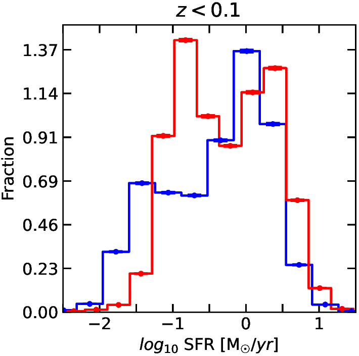
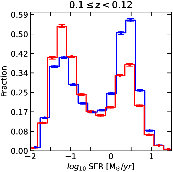
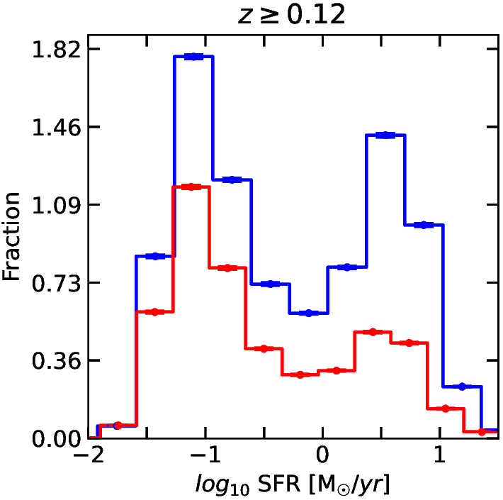
Figure 3: Star formation rate distributions for isolated (blue solid line) galaxies and group galaxies (red solid line). The error bars are 1 $\sigma$ Poissonian errors.

           

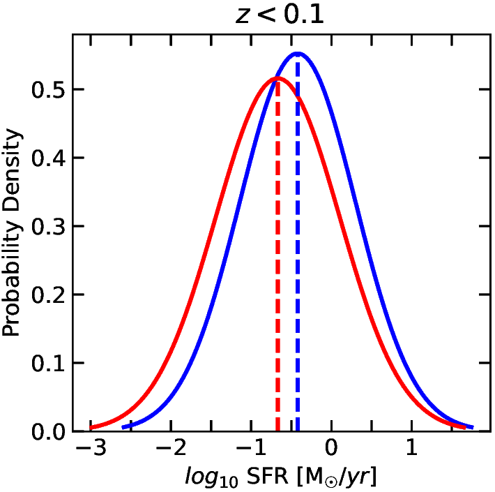
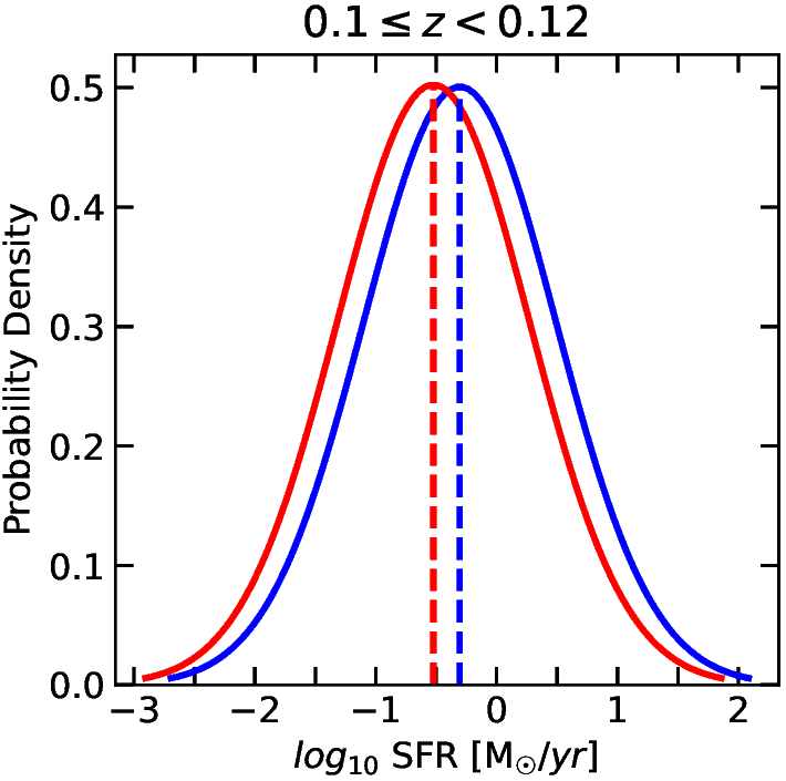
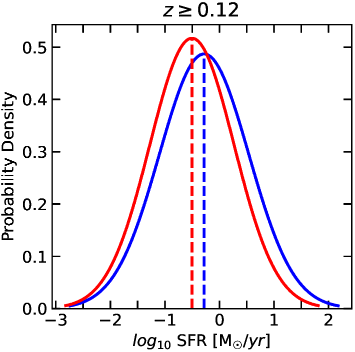
Figure 4: Star formation rate distribution curves as obtained from the Gaussian fitting for isolated galaxies (blue solid line) and group galaxies (red solid line). Blue and red dotted lines show the position of the median of distributions for isolated and group galaxies respectively.

Figures 3 and 5 show the general distributions of SFR and SSFR, respectively within the redshift range of $z<0.1$, $0.1\leq z<0.12$, and $z\geq 0.12$ for galaxies in both isolated and group environments. The corresponding Gaussian distributions of SFR and SSFR in both these galaxy environments are illustrated in Figures 4 and 6 respectively. As depicted in Figure 4, and columns (4), (5) of Table 1, galaxies in isolated environments tend to have higher SFR than in group environments. Similarly, from Figure 6, and columns (6), (7) of Table 1, it is also evident that galaxies exhibit low SSFR in group environments across all redshift bins compared to isolated environments. The middle plot of Figure 7 indicates that the SFR increases gradually with the increase in redshift with isolated galaxies having higher SFR than isolated galaxies. However, it is seen that the SFR increases rapidly for galaxies located in low redshift ($z\leq 0.05$) regions than the high redshift regions. In contrast, the right plot of Figure 7 indicates that the SSFR decreases with the increase in redshift with isolated galaxies having higher SSFR than group galaxies. The observed consistency of SFR and SSFR in isolated and group environments supports the perspective that galaxies generally display high SFR and SSFR in low-density regions, and low SFR and SSFR in high-density regions of the Universe, that high-density environments tend to inhibit the process of star formation indicated by many possible mechanisms such as supernova explosion, magnetic fields, stellar winds, and radiation pressure [7, 21, 28, 22, 16, 23]. Moreover, the observation from Figures 1, 3, and 5 indicate that at high redshift bins $(z\geq 0.12)$, the sample in isolated environments has a higher proportion of galaxies, whereas, at low redshift bins $(z<0.1)$, the sample in group environments has a higher proportion of galaxies, for intermediate redshift $(0.1\leq z<0.12)$ an approximately equal proportional of galaxies is observed.

           

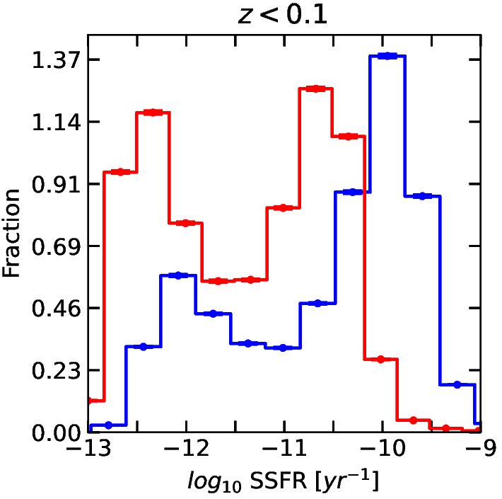
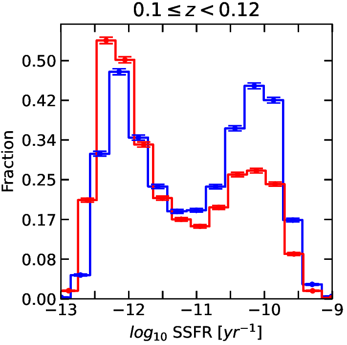
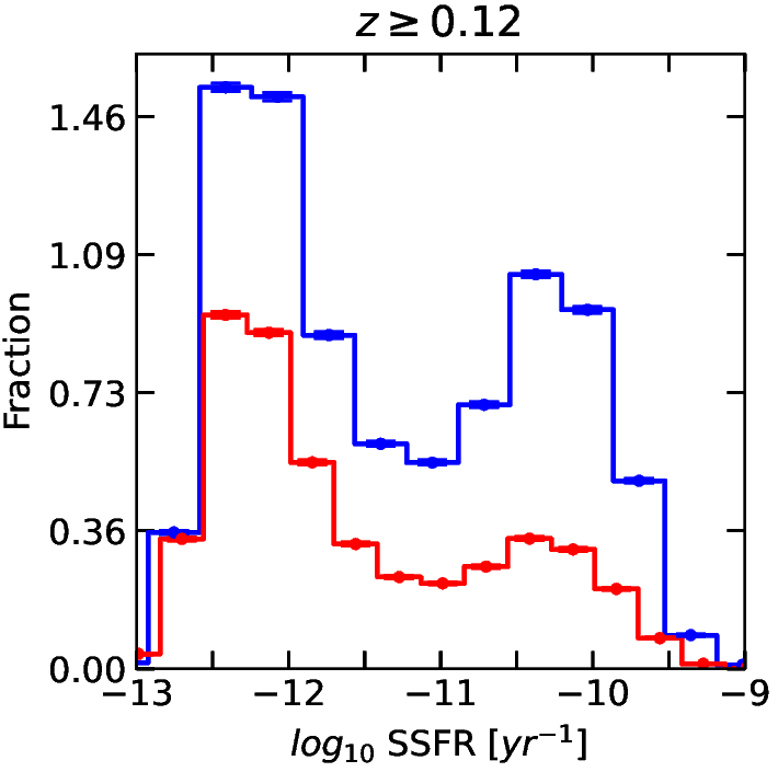
Figure 5: Specific star formation rate distribution for isolated galaxies (blue solid line) and group galaxies (red solid line). The error bars are 1 $\sigma$ Poissonian errors.

           

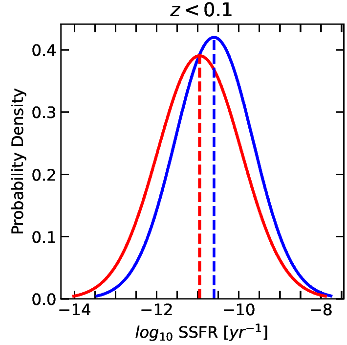
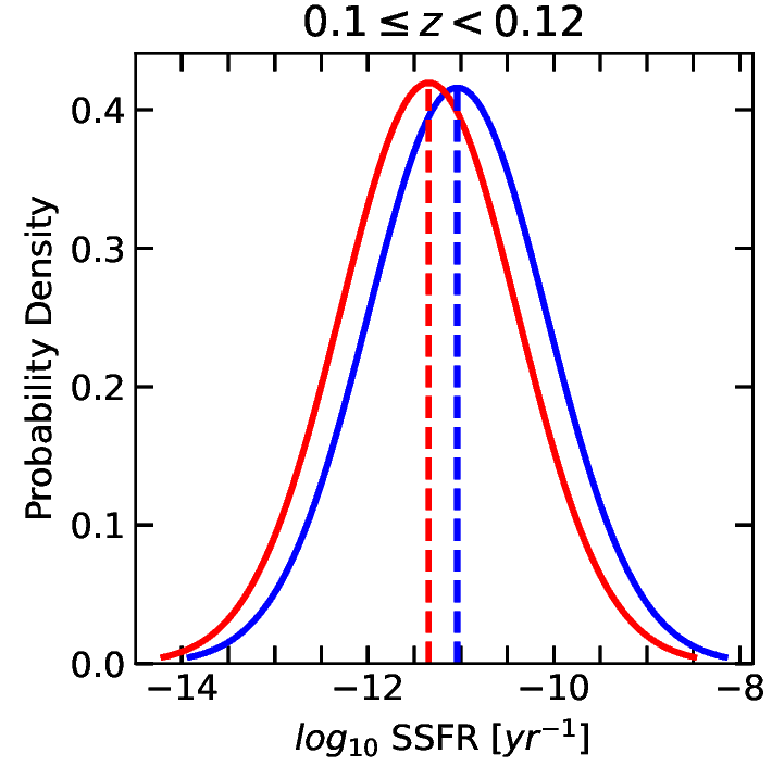
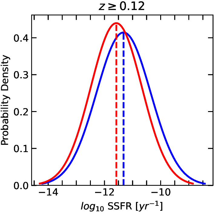
Figure 6: Specific star formation rate distribution curves as obtained from the Gaussian fitting for isolated galaxies (blue solid line) and group galaxies (red solid line). Blue and red dotted lines show the position of the mean for isolated, and group galaxies respectively.

The Kolmogorov-Smirnov (KS) test Ref. [34], serves as a quantitative comparison, assessing the degree of similarity or difference between two independent distributions by calculating a probability value. This probability value indicates the likelihood that the two distributions are derived from the same parent distribution. A high probability suggests a high likelihood of the two distributions sharing a common parent, while a low probability implies that the distributions are different. The calculated probabilities, listed in Table 2, are between $3.40\times 10^{-203}$ and $3.02\times 10^{-59}$ for stellar mass, between $1.61\times 10^{-302}$ and $9.95\times 10^{-67}$ for SFR, similarly between $0$ and $3.39\times 10^{-71}$ for SSFR, which are notably much less than 0.05 $(5\%)$, a standard threshold in statistical analysis. This outcome suggests that the two independent distributions in each of Figures 1, 3, and 5 are significantly different, reinforcing that a strong correlation exists between the environment, stellar mass, SFR, and SSFR. These findings support the assertion of a robust environmental dependence of stellar mass, SFR, and SSFR in all redshift bins within the sample. Consequently, there is substantial confidence in accepting this conclusion.

           

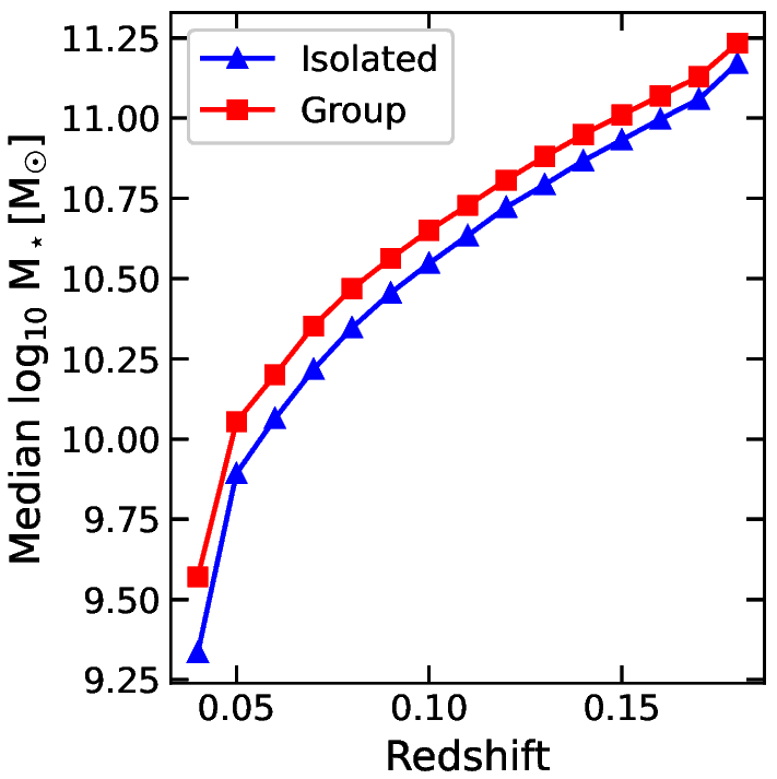
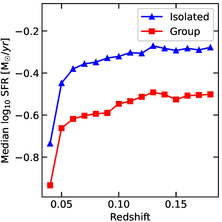
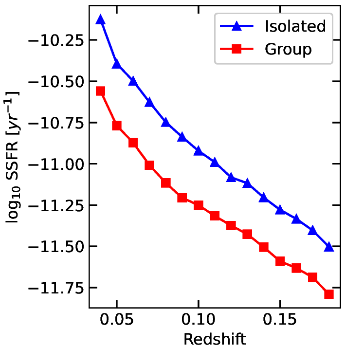
Figure 7: Variation of median stellar mass (left plot), SFR (middle plot), and SSFR (right plot) with redshift for isolated galaxies (blue solid line) and group galaxies (red solid line).

Table 1: Mean stellar mass, mean SFR and mean SSFR for isolated and group galaxies within the redshift bin size of $\Delta z=0.01$. The associated uncertainty is the standard error in the measurement.

Redshift	log10 M${}_{\star}[M_{\odot}]$		log10 SFR$[M_{\odot}/yr$]		log10 SSFR$[yr^{-1}]$
	Isolated	Group	Isolated	Group	Isolated	Group
(1)	(2)	(3)	(4)	(5)	(6)	(7)
$z<0.04$	$9.34\pm 0.005$	$9.57\pm 0.004$	$-0.74\pm 0.004$	$-0.93\pm 0.004$	$-10.13\pm 0.005$	$-10.56\pm 0.005$
$0.04\leq z<0.05$	$9.89\pm 0.005$	$10.05\pm 0.004$	$-0.45\pm 0.006$	$-0.66\pm 0.005$	$-10.39\pm 0.008$	$-10.77\pm 0.008$
$0.05\leq z<0.06$	$10.06\pm 0.004$	$10.20\pm 0.004$	$-0.38\pm 0.006$	$-0.62\pm 0.006$	$-10.50\pm 0.008$	$-10.87\pm 0.008$
$0.06\leq z<0.07$	$10.22\pm 0.003$	$10.35\pm 0.003$	$-0.36\pm 0.005$	$-0.60\pm 0.005$	$-10.63\pm 0.007$	$-11.01\pm 0.007$
$0.07\leq z<0.08$	$10.35\pm 0.003$	$10.46\pm 0.002$	$-0.35\pm 0.005$	$-0.59\pm 0.005$	$-10.75\pm 0.006$	$-11.12\pm 0.006$
$0.08\leq z<0.09$	$10.45\pm 0.002$	$10.56\pm 0.002$	$-0.33\pm 0.005$	$-0.59\pm 0.005$	$-10.84\pm 0.007$	$-11.21\pm 0.006$
$0.09\leq z<0.10$	$10.54\pm 0.002$	$10.65\pm 0.002$	$-0.32\pm 0.005$	$-0.55\pm 0.005$	$-10.92\pm 0.007$	$-11.25\pm 0.007$
$0.10\leq z<0.11$	$10.63\pm 0.002$	$10.72\pm 0.002$	$-0.30\pm 0.005$	$-0.53\pm 0.005$	$-10.99\pm 0.007$	$-11.32\pm 0.007$
$0.11\leq z<0.12$	$10.72\pm 0.002$	$10.80\pm 0.002$	$-0.31\pm 0.005$	$-0.51\pm 0.006$	$-11.08\pm 0.007$	$-11.37\pm 0.007$
$0.12\leq z<0.13$	$10.79\pm 0.002$	$10.88\pm 0.002$	$-0.27\pm 0.006$	$-0.49\pm 0.006$	$-11.12\pm 0.007$	$-11.43\pm 0.007$
$0.13\leq z<0.14$	$10.86\pm 0.002$	$10.94\pm 0.002$	$-0.28\pm 0.006$	$-0.50\pm 0.006$	$-11.20\pm 0.007$	$-11.50\pm 0.008$
$0.14\leq z<0.15$	$10.93\pm 0.002$	$11.00\pm 0.002$	$-0.29\pm 0.006$	$-0.53\pm 0.007$	$-11.28\pm 0.007$	$-11.59\pm 0.009$
$0.15\leq z<0.16$	$10.99\pm 0.002$	$11.06\pm 0.003$	$-0.28\pm 0.006$	$-0.51\pm 0.008$	$-11.33\pm 0.008$	$-11.63\pm 0.010$
$0.16\leq z<0.17$	$11.05\pm 0.002$	$11.12\pm 0.003$	$-0.29\pm 0.007$	$-0.50\pm 0.009$	$-11.40\pm 0.008$	$-11.69\pm 0.011$
$z\geq 0.17$	$11.17\pm 0.001$	$11.23\pm 0.002$	$-0.28\pm 0.001$	$-0.50\pm 0.007$	$-11.50\pm 0.005$	$-11.79\pm 0.008$

IV Conclusion

In this study, we utilized the galaxy sample from SDSS DR12, specifically the value-added catalogue by Ref. [13], consisting of 584,449 galaxies. The MPA-JHU measurements were used to investigate the impact of isolated and group environments on stellar mass, SFR, and SSFR. To mitigate the Malmquist bias, the entire sample was divided into fifteen subsamples with a redshift binning size of $\Delta z=0.01$. We analyzed the properties of these subsamples in each redshift bin for both isolated and group environments. The results, as depicted in Figures 1, 2, 3, 4, 5, 6, 7, and detailed in Table 1, provide the valuable insights. Additionally, the KS test results shown in Table 2 align with the conclusions drawn from the histogram figures, reinforcing the statistical significance of the findings. The key findings of this study are:

Table 2: KS probabilities for stellar mass, SFR and SSFR.

Redshift	P (Stellar Mass)	P (SFR)	P (SSFR)
(1)	(2)	(3)	(4)
$z<0.04$	$3.40e-203$	$1.61e-302$	$0$
$0.04\leq z<0.05$	$1.29e-72$	$1.24e-193$	$1.13e-212$
$0.05\leq z<0.06$	$1.97e-71$	$2.17e-210$	$2.19e-212$
$0.06\leq z<0.07$	$2.12e-111$	$5.50e-275$	$7.36e-277$
$0.07\leq z<0.08$	$8.40e-130$	$1.63e-130$	$3.05e-316$
$0.08\leq z<0.09$	$9.72e-126$	$2.90e-283$	$2.96e-298$
$0.09\leq z<0.10$	$1.19e-106$	$2.87e-186$	$8.93e-200$
$0.10\leq z<0.11$	$1.68e-106$	$2.93e-178$	$3.11e-192$
$0.11\leq z<0.12$	$1.06e-107$	$5.84e-151$	$6.94e-169$
$0.12\leq z<0.13$	$1.54e-109$	$2.97e-137$	$1.33e-153$
$0.13\leq z<0.14$	$3.98e-112$	$6.47e-130$	$7.58e-147$
$0.14\leq z<0.15$	$3.47e-79$	$4.42e-112$	$1.91e-122$
$0.15\leq z<0.16$	$2.42e-65$	$8.24e-86$	$1.30e-92$
$0.16\leq z<0.17$	$3.02e-59$	$9.95e-67$	$3.39e-71$
$z\geq 0.17$	$1.21e-73$	$3.50e-100$	$1.55e-111$

• High-mass galaxies tend to exist in groups across all redshift bins, while low-mass galaxies show a preference for isolated environments. This is consistent with previous conclusions regarding galaxy distributions in high and low-density regions, that high-mass galaxies exist in the high-density region of the Universe while low-mass galaxies exist in the low-density region of the Universe [8, 9].

• Galaxies in group environments exhibit lower SFR and SSFR across all redshift bins, whereas galaxies in isolated environments tend to have higher SFR and SSFR. This aligns with the conclusion from other studies that galaxies display higher SFR, SSFR in low-density regions of the Universe, and low SFR, SSFR in higher-density regions of the Universe [7, 21, 28, 22, 16, 23].

• The stellar mass, and SFR increase with the increase in redshift while the SSFR decreases with the increase in redshift for both isolated and group galaxies.

• The proportion of galaxies within isolated and group environments depends on the redshift values. In the lower redshift bins ($z<0.1$), the galaxys proportion is higher in isolated environments than in the group environments. In the intermediate redshift bins ($0.1\leq z<0.12$) galaxies have almost equal proportionality in both environments. Whereas in the higher redshift bins ($z\geq 0.12$) the proportionality of galaxies is higher in the group environments than in the isolated environments.

• The KS test results provide statistical support for the observed differences in distributions, reinforcing the robustness of the study’s conclusions.

These findings contribute to a more profound comprehension of the intricate interplay between stellar mass, SFR, and SSFR, influenced by the environmental conditions of galaxies. The study not only reveals patterns in the distribution of these properties across different redshift bins but also underscores the significant impact that isolation and group environments have on the observed characteristics of galaxies.

In the future, we hope to examine the evolution of the physical properties (e.g., stellar mass and SFR) for emission line and morphologically classified galaxies in different local environments (e.g., isolated, group and cluster), and interpret the results more quantitatively studying the influence of AGN on the observed properties.

References

- [1] M. Einasto, H. Lietzen, E. Tempel, M. Gramann SDSS superclusters: morphology and galaxy contents, Astronomy & Astrophysics 562, A87 (2014) [arXiv:1401.3226].
- [2] C. Conroy Modeling the Panchromatic Spectral Energy Distributions of Galaxies, Annual Review of Astronomy and Astrophysics 51, 393–455 (2013) [arXiv:1301.7095].
- [3] R. Smethurst, C. Lintott, S. Bamford, R. Hart, S. Kruk, K. Masters, Galaxy Zoo: The interplay of quenching mechanisms in the group environment, Monthly Notices of the Royal Astronomical Society 469, 3670–3687 (2009) [arXiv:1704.06269].
- [4] L. Kewley, B. Groves, G. Kauffmann, T. Heckman, The host galaxies and classification of active galactic nuclei, Monthly Notices of the Royal Astronomical Society 372, 961–976 (2006) [arXiv:astro-ph/0605681].
- [5] B. Terrazas, E. Bell, B. Henriques, S. White, A. Cattaneo, J. Woo Quiescence correlates strongly with directly-measured black hole mass in central galaxies, The Astrophysical journal letters 830, L12 (2016) [arXiv:1609.07141].
- [6] Y. Peng, S. Lilly, K. Kovač, M. Bolzonella, L. Pozzetti, A. Renzini, G. Zamorani, Mass and Environment as Drivers of Galaxy Evolution in SDSS and zCOSMOS and the Origin of the Schechter Function, The Astrophysical Journal 721, 193 (2010) [arXiv:1003.4747].
- [7] I. Lewis, M. Balogh, R. Propris, W. Couch, R. Bower, The 2dF Galaxy Redshift Survey: the environmental dependence of galaxy star formation rates near clusters, Monthly Notices of the Royal Astronomical Society 334, 673–683 (2002) [arXiv:astro-ph/0203336].
- [8] G. Kauffmann, S. White, The Environmental Dependence of the Relations between Stellar Mass, Structure, Star Formation and Nuclear Activity in Galaxies, Monthly Notices of the Royal Astronomical Society 353, 713–731 (2004) [arXiv:astro-ph/0402030].
- [9] C. Li, G. Kauffmann, Y. Jing, S. White, The dependence of clustering on galaxy properties, Monthly Notices of the Royal Astronomical Society 368, 21–36 (2006) [arXiv:astro-ph/0509873].
- [10] D. Eisenstein, D. Weinberg, SDSS-III: Massive spectroscopic surveys of the distant universe, the Milky Way, and extra-solar planetary systems, The Astronomical Journal 142, 72 (2011) [arXiv:1101.1529].
- [11] S. Alam, F. Albareti, C. Prieto, The Eleventh and Twelfth Data Releases of the Sloan Digital Sky Survey: Final Data from SDSS-III, The Astrophysical Journal Supplement Series 219, 12 (2015) [arXiv:1501.00963].
- [12] N. Abdurro’uf, K. Accetta, C. Aerts, The Seventeenth Data Release of the Sloan Digital Sky Surveys: Complete Release of MaNGA, MaStar and APOGEE-2 Data, The Astrophysical Journal Supplement Series 259, 1 (2022) [arXiv:2112.02026].
- [13] E. Tempel, T. Tuvikene, Merging groups and clusters of galaxies from the SDSS data. The catalogue of groups and potentially merging systems, Astronomy & Astrophysics 602, A100 (2017) [arXiv:1704.04477].
- [14] R. Grützbauch, R. Chuter, Galaxy properties in different environments up to in the GOODS NICMOS Survey, Monthly Notices of the Royal Astronomical Society 412, 2361–2375 (2011) [arXiv:1011.4846].
- [15] M. Cooper, J. Newman, The DEEP2 Galaxy Redshift Survey: The Relationship Between Galaxy Properties and Environment at , Monthly Notices of the Royal Astronomical Society 370, 198–212 (2006) [arXiv:astro-ph/0603177].
- [16] M. Cooper, J. Newman, The DEEP2 Galaxy Redshift Survey: The Role of Galaxy Environment in the Cosmic Star-Formation History, Monthly Notices of the Royal Astronomical Society 383, 1058–1078 (2008) [arXiv:0706.4089].
- [17] J. Brinchmann, S. Charlot, The physical properties of star forming galaxies in the low redshift universe, Monthly Notices of the Royal Astronomical Society 351, 1151–1179 (2004) [arXiv:astro-ph/0311060].
- [18] S. Salim, J. Lee, R. Davé, On the Mass-Metallicity-Star Formation Rate Relation for Galaxies at , The Astrophysical Journal 808, 14pp (2015) [arXiv:1506.03080].
- [19] P. Ade, N. Aghanim, Planck 2015 results. XXIII. The thermal Sunyaev-Zeldovich effect–cosmic infrared background correlation, Astronomy & Astrophysics 594, A23 (2016) [arXiv:1509.06555].
- [20] J. Etherington, D. Thomas, Environmental dependence of the galaxy stellar mass function in the Dark Energy Survey Science Verification Data, Astronomy & Astrophysics 466, 228–247 (2016) [arXiv:1701.06066].
- [21] P. Gomez, R. Nichol, Galaxy Star-Formation as a Function of Environment in the Early Data Release of the Sloan Digital Sky Survey, Astronomy & Astrophysics 584, 210 (2003) [arXiv:astro-ph/0210193].
- [22] D. Elbaz, E. Daddi, D. Borgne, The reversal of the star formation-density relation in the distant universe, Astronomy & Astrophysics 468, 33–48 (2007) [arXiv:astro-ph/0703653].
- [23] S. Patel, B. Holden, The Dependence of Star Formation Rates on Stellar Mass and Environment at , The Astrophysical Journal 705, L67 (2007) [arXiv:0910.0837].
- [24] Y. Yoon, J. Kim, Low-mass Quiescent Galaxies Are Small in Isolated Environments: Environmental Dependence of the Mass-Size Relation of Low-mass Quiescent Galaxies, The Astrophysical Journal 957, 59 (2023) [arXiv:2310.07498].
- [25] J. Scudder, S. Ellison,The dependence of galaxy group star formation rates and metallicities on large-scale environment, The Astrophysical Journal 423, 2690–2704 (2012) [arXiv:1204.2828].
- [26] S. Sankhyayan, J. Bagchi,Identification of Superclusters and their Properties in the Sloan Digital Sky Survey Using WHL Cluster Catalog, The Astrophysical Journal 958, 62 (2023) [arXiv:2309.06251].
- [27] S. Bag, L. Liivamägi, M. Einasto,The shape distribution of superclusters in SDSS DR 12, Monthly Notices of the Royal Astronomical Society 521, 4712 – 4730 (2023) [arXiv:2111.10253].
- [28] M. Tanaka, T. Goto,The Environmental Dependence of Galaxy Properties in the Local Universe: Dependence on Luminosity, Local Density, and System Richness, The Astronomical Journal 128, 2677 (2004) [arXiv:astro-ph/0411132].
- [29] N. Ball, J. Loveday, Galaxy Colour, Morphology, and Environment in the Sloan Digital Sky Survey, Monthly Notices of the Royal Astronomical Society 383, 907–922 (2008) [arXiv:astro-ph/0610171].
- [30] P. Teerikorp, Eddington-Malmquist bias in a cosmological context, Astronomy & Astrophysics576, A75 (2015) [arXiv:1503.02812].
- [31] C. Tremonti, T. Heckman,The Origin of the Mass–Metallicity Relation: Insights from 53,000 Star-Forming Galaxies in the SDSS, The Astrophysical Journal 613, 898 (2004) [arXiv:astro-ph/0405537].
- [32] D. York, J. Adelman, The sloan digital sky survey: Technical summary, The Astronomical Journal 120, 1579 (2000) [arXiv:astro-ph/0006396].
- [33] E. Tempel, A. Tamm, M. Gramann, Flux- and volume-limited groups/clusters for the SDSS galaxies: catalogues and mass estimation, Astronomy & Astrophysics 566, A1 (2014) [arXiv:1402.1350].
- [34] D. Harari, S. Mollerach, Kolmogorov-Smirnov test as a tool to study the distribution of ultra-high energy cosmic ray sources, Astronomy & Astrophysics 394, 916–922 (2009) [arXiv:0811.0008].