Local modification of subdiffusion by initial Fickian diffusion: Multiscale modeling, analysis and computation

Abstract

We propose a local modification of the standard subdiffusion model by introducing the initial Fickian diffusion, which results in a multiscale diffusion model. The developed model resolves the incompatibility between the nonlocal operators in subdiffusion and the local initial conditions and thus eliminates the initial singularity of the solutions of the subdiffusion, while retaining its heavy tail behavior away from the initial time. The well-posedness of the model and high-order regularity estimates of its solutions are analyzed by resolvent estimates, based on which the numerical discretization and analysis are performed. Numerical experiments are carried out to substantiate the theoretical findings.

1 Introduction

We consider the subdiffusion model with the variable exponent [7, 8, 10, 11, 14, 27, 29], which has been used in various fields such as the transient dispersion in heterogeneous media [23] (more applications could be found in the review [24])

$$\begin{array}[]{c}\partial_{t}u(\bm{x},t)-\partial_{t}^{\alpha(t)}\Delta u(\bm{x},t)=f(\bm{x},t),~{}~{}(\bm{x},t)\in\Omega\times(0,T];\\[3.61371pt] \displaystyle u(\bm{x},0)=u_{0}(\bm{x}),~{}\bm{x}\in\Omega;\quad u(\bm{x},t)=0,~{}(\bm{x},t)\in\partial\Omega\times[0,T].\end{array}$$ (1)

Here $\Omega\subset\mathbb{R}^{d}$ is a simply-connected bounded domain with the piecewise smooth boundary $\partial\Omega$ with convex corners, $\bm{x}:=(x_{1},\cdots,x_{d})$ with $1\leq d\leq 3$ denotes the spatial variables, $f$ and $u_{0}$ refer to the source term and the initial value, respectively, and $\partial_{t}^{\alpha(t)}$ with the variable exponent $0\leq\alpha(t)<1$ is the Riemann-Liouville fractional differential operator defined by the symbol $*$ of convolution [16]

$$\displaystyle\partial_{t}^{\alpha(t)}u:=\partial_{t}\,I_{t}^{1-\alpha(t)}u,\qquad I_{t}^{1-\alpha(t)}u:=\Big{(}\frac{t^{-\alpha(t)}}{\Gamma(1-\alpha(t))}\Big{)}*u(\bm{x},t).$$ (2)

1.1 Modeling issues

In this work, we explore more benefits and properties of (1) via rigorous analysis. A key ingredient lies in that we require $\alpha(0)=0$, that is, we expect the model (1) to degenerate to its integer-order analogue at the time instant $t=0$ in order to resolve the incompatibility between the nonlocal operators in subdiffusion and the local initial conditions, as mentioned in [26]. If such local modification works, the model (1) indeed exhibits multiple diffusion scales, i.e. the Fickian diffusion near the initial time and the subdiffusion away from the initial time.

To give an intuitive motivation, we compare the solutions of the multiscale diffusion model (1) with its integer-order analogue, i.e. model (1) with $\alpha(t)\equiv 0$, which models the purely Fickian diffusion

$$\partial_{t}u(\bm{x},t)-\Delta u(\bm{x},t)=f(\bm{x},t)$$

and its constant-exponent analogue, i.e. model (1) with $\alpha(t)\equiv\bar{\alpha}$ for some $0<\bar{\alpha}<1$, which accurately captures the power-law decaying property of the purely subdiffusion through heterogeneous porous media [18, 19] and has attracted extensive research activities [3, 4, 5, 9, 15, 21, 22]

$$\partial_{t}u(\bm{x},t)-\partial_{t}^{\bar{\alpha}}\Delta u(\bm{x},t)=f(\bm{x},t).$$ (3)

The solution curves of the above three models are presented in Figure 1, from which we observe that:

• In comparison with the solution curves of the purely Fickian diffusion and subdiffusion, the solutions to model (1) transit from the initial Fickian diffusion behavior to the long-term subdiffusion behavior, which indicates the multiscale feature of this model.

• Compared with the initial rapid change (i.e. the initial singularity) of the solutions to the purely subdiffusion, the solutions to the multiscale diffusion model (1) exhibits the Fickian diffusion behavior near the initial time, which eliminates the incompatibility between the nonlocal operators in subdiffusion and the local initial conditions.

• Compared with the exponential decay of the solutions to the purely Fickian diffusion away from the initial time, the solutions to the multiscale diffusion model (1) exhibits the subdiffusion behavior, which retains the advantages of the subdiffusion in modeling the power law decay and heavy tail behavior.

In summary, the multiscale diffusion model (1) provides a framework incorporating both Fickian and subdiffusion models and simultaneously retaining their features and advantages, which indicates the superiority of model (1) and motivates the current study on its mathematical and numerical analysis.

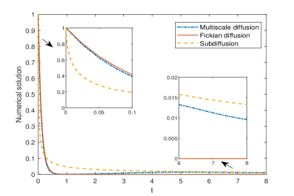
Fig. 1: Plots of the solutions $u(0.5,t)$ for three models under $\Omega=(0,1)$, $T=8$, $f\equiv 0$, $u_{0}=\sin(\pi x)$. Here the variable exponent is chosen as $\alpha(t)=\alpha(T)+(\alpha(0)-\alpha(T))\big{(}1-\frac{t}{T}-\frac{\sin(2\pi(1-t/T))}{2\pi}\big{)}$, a smooth and monotonic function on $[0,T]$ with end values $\alpha(0)=0$ and $\alpha(T)=0.4$. We accordingly fix $\bar{\alpha}=0.4$.

1.2 Analysis issues

There exist rare investigations for analysis of variable-exponent fractional partial differential equations in the literature. Recently, there are some progresses on the mathematical and numerical analysis of variable-exponent mobile-immobile time-fractional diffusion equations [12, 13, 26, 28], a different model from (1)

$$\partial_{t}u(\bm{x},t)+k\,\partial_{t}^{\alpha(t)}u(\bm{x},t)-\Delta u(\bm{x},t)=f(\bm{x},t).$$ (4)

Though different methods have been developed to study (4), all derivations are based on a critical fact that the $\partial_{t}u(\bm{x},t)$ in (4) dominates the $\partial_{t}^{\alpha(t)}u(\bm{x},t)$ such that the later could be considered as a low-order or perturbation term. In this case, the effects of variable-exponent fractional operators, which do not have nice properties as constant-exponent operators, are weakened. However, this phenomenon does not appear in (1) due to the composition of temporal and spatial operators, which brings essential differences and difficulties in comparison with (4).

In this work, we derive an equivalent model as (1), which paves the way to perform analysis. Based on this more feasible formulation, we prove the well-posedness and regularity of the solutions, as well as developing and analyzing the fully-discrete finite element scheme. The rest of the paper is organized as follows: In §2, we introduce the notations and preliminary results to be used subsequently. In §3, we prove the well-posedness of the multiscale diffusion model and the regularity estimates of its solutions. In §4, we prove high-order regularity of the solutions via resolvent estimates. In §5, we derive a fully-discrete finite element scheme to the model and prove its error estimates. Numerical experiments are performed in §6 to substantiate the theoretical findings.

2 Preliminaries

We present preliminaries to be used subsequently.

2.1 Notations

Let $L^{p}(\Omega)$ with $1\leq p\leq\infty$ be the Banach space of $p$th power Lebesgue integrable functions on $\Omega$. For a positive integer $m$, let $W^{m,p}(\Omega)$ be the Sobolev space of $L^{p}$ functions with $m$th weakly derivatives in $L^{p}(\Omega)$ (similarly defined with $\Omega$ replaced by an interval $\mathcal{I}$). Let $H^{m}(\Omega):=W^{m,2}(\Omega)$ and $H^{m}_{0}(\Omega)$ be its subspace with the zero boundary condition up to order $m-1$. For a non-integer $s\geq 0$, $H^{s}(\Omega)$ is defined via interpolation [1]. Let $0<\lambda_{i}\uparrow\infty$ be the eigenvalues and $\{\phi_{i}\}_{i=1}^{\infty}$ be the corresponding orthonormal eigenfunctions of the problem $-\Delta\phi_{i}=\lambda_{i}\phi_{i}$ with the zero boundary condition. We introduce the Sobolev space $\check{H}^{s}(\Omega)$ for $s\geq 0$ by

$$\check{H}^{s}(\Omega):=\bigg{\{}v\in L^{2}(\Omega):\|v\|_{\check{H}^{s}}^{2}:=\sum_{i=1}^{\infty}\lambda_{i}^{s}(v,\phi_{i})^{2}<\infty\bigg{\}},$$

which is a subspace of $H^{s}(\Omega)$ satisfying $\check{H}^{0}(\Omega)=L^{2}(\Omega)$ and $\check{H}^{2}(\Omega)=H^{2}(\Omega)\cap H^{1}_{0}(\Omega)$ [25]. For a Banach space $\mathcal{X}$, let $W^{m,p}(0,T;\mathcal{X})$ be the space of functions in $W^{m,p}(0,T)$ with respect to $\|\cdot\|_{\mathcal{X}}$. All spaces are equipped with standard norms [1, 6].

We use $Q$, $Q_{i}$ and $Q_{*}$ to denote generic positive constants in which $Q$ may assume different values at different occurrences. We set $\|\cdot\|:=\|\cdot\|_{L^{2}(\Omega)}$ and $L^{p}(\mathcal{X})$ for $L^{p}(0,T;\mathcal{X})$ for brevity, and drop the notation $\Omega$ in the spaces and norms if no confusion occurs.

We make the Assumption A throughout this paper:

• $0\leq\alpha(t)\leq\alpha^{*}<1$ and $|\alpha^{\prime}(t)|$, $|\alpha^{\prime\prime}(t)|\leq Q_{*}$ on $[0,T]$. In addition, $\alpha(0)=0$.

• $f\in L^{p}(L^{2})$ for $1<p<\infty$ and $u_{0}\in\check{H}^{2}$.

2.2 Solution representation and resolvent estimates

For $\theta\in(\pi/2,\pi)$ and $\delta>0$, let $\Gamma_{\theta}$ be the contour in the complex plane defined by

$$\Gamma_{\theta}:=\big{\{}z\in\mathbb{C}:|{\rm arg}(z)|=\theta,|z|\geq\delta\big{\}}\cup\big{\{}z\in\mathbb{C}:|{\rm arg}(z)|\leq\theta,|z|=\delta\big{\}}.$$

The following inequalities hold for $0<\mu\leq 1$ and $Q=Q(\theta,\mu)$ [2, 17]

$$\int_{\Gamma_{\theta}}|z|^{\mu-1}|e^{tz}|\,|dz|\leq Qt^{-\mu},~{}~{}\bigg{\|}\int_{\Gamma_{\theta}}z^{\mu}(z-\Delta)^{-1}e^{tz}\,dz\bigg{\|}_{L^{2}\rightarrow L^{2}}\leq\frac{Q}{t^{\mu}},~{}~{}t\in(0,T].$$ (5)

For any $q\in L^{1}_{loc}(\mathcal{I})$, the Laplace transform $\mathcal{L}$ of its extension $\tilde{q}(t)$ to zero outside $\mathcal{I}$ and the corresponding inverse transform $\mathcal{L}^{-1}$ are denoted by

$$\begin{array}[]{l}\displaystyle\mathcal{L}q(z):=\int_{0}^{\infty}\tilde{q}(t)e^{-tz}dt,\qquad\mathcal{L}^{-1}(\mathcal{L}q(z)):=\frac{1}{2\pi\rm i}\int_{\Gamma_{\theta}}e^{tz}\mathcal{L}q(z)dz=q(t),\\[10.84006pt] \displaystyle\mathcal{L}\big{(}{}^{R}\partial_{t}^{\gamma}q(t)\big{)}=z^{\gamma}\mathcal{L}\big{(}q(t)\big{)},\quad{}^{R}\partial_{t}^{\gamma}q:=\partial_{t}\,I_{t}^{1-\gamma}q,\qquad 0\leq\gamma<1.\end{array}$$ (6)

Let $E(t):=e^{t\Delta}$ be the semigroup generated by the Dirichlet Laplacian. The solution $u$ to the heat equation

$$\begin{array}[]{c}\displaystyle\partial_{t}u(\bm{x},t)-\Delta u(\bm{x},t)=f(\bm{x},t),~{}~{}(\bm{x},t)\in\Omega\times(0,T],\\[3.61371pt] u(\bm{x},t)=0,\quad(\bm{x},t)\in\partial\Omega\times(0,T],~{}~{}u(\bm{x},0)=0,~{}~{}\bm{x}\in\Omega\end{array}$$ (7)

can be expressed in terms of the $E(t)$ via the Duhamel’s principle

$$u(\bm{x},t)=\int_{0}^{t}E(t-\theta)f(\bm{x},\theta)d\theta,$$ (8)

where $E(t)$ has the spectral decomposition and expression in terms of the inverse Laplace transform

$$E(t)\psi(\bm{x})=\sum_{i=1}^{\infty}e^{-\lambda_{i}t}(\psi,\phi_{i})\phi_{i}(\bm{x})=\frac{1}{2\pi{\rm i}}\int_{\Gamma_{\theta}}e^{zt}(z-\Delta)^{-1}\psi(\bm{x})\,dz,~{}~{}\psi\in L^{2}(\Omega).$$ (9)

The following estimates hold for $s\geq r\geq-1$ and for any $t>0$ [2, 17, 25]

$$\begin{array}[]{l}\displaystyle\|E(t)\|_{L^{2}\to L^{2}}\leq Q,\quad\displaystyle\|E(t)\psi\|_{\check{H}^{s}}\leq Qt^{-(s-r)/2}\|\psi\|_{\check{H}^{r}},\qquad\psi\in\check{H}^{r}.\end{array}$$ (10)

Lemma 2.1.

[2] If $f\in L^{p}(L^{2})$ for $1<p<\infty$, problem (7) has a unique solution $u\in W^{1,p}(L^{2})\cap L^{p}(\check{H}^{2})$ given by (8) such that

$$\|u\|_{W^{1,p}(0,t;L^{2})}+\|u\|_{L^{p}(0,t;\check{H}^{2})}\leq Q\|f\|_{L^{p}(0,t;L^{2})},~{}~{}0<t\leq T,$$

where $Q$ is independent of $f$, $t$ or $T$.

We finally apply (14) to introduce the following relations which will be used frequently in subsequent analysis [20]

$$\begin{array}[]{l}\displaystyle(t-s)^{-\alpha(t-s)}=e^{-\alpha(t-s)\ln(t-s)}\leq Q,\\[5.42003pt] \displaystyle\int_{0}^{T}e^{-\gamma t}t^{-\mu}dt\leq\gamma^{\mu-1}\int_{0}^{\infty}e^{-s}s^{-\mu}ds=\gamma^{\mu-1}\Gamma(1-\mu),\quad\mu<1.\end{array}$$ (11)

3 Well-posedness

3.1 Model reformulation

We give an equivalent but more feasible formulation of the multiscale diffusion model (1) to facilitate the analysis.

Theorem 3.1.

If $u$ solves the multiscale diffusion model (1), then $u$ solves the following system

$$\begin{array}[]{c}\displaystyle\partial_{t}u(\bm{x},t)-\Delta u(\bm{x},t)=f(\bm{x},t)+B(t)u(\bm{x},t),~{}~{}(\bm{x},t)\in\Omega\times(0,T];\\[3.61371pt] \displaystyle u(\bm{x},0)=u_{0}(\bm{x}),~{}\bm{x}\in\Omega;\quad u(\bm{x},t)=0,~{}(\bm{x},t)\in\partial\Omega\times[0,T]\end{array}$$ (12)

where

$$B(t)u:=g(t)*\Delta u\text{ with }g(t):=\partial_{t}\Big{(}\frac{t^{-\alpha(t)}}{\Gamma(1-\alpha(t))}\Big{)}.$$

Conversely, if $u$ solves (12), then $u$ solves the multiscale diffusion model (1).

Proof.

We first prove the problem (1) could be reformulated to (12). We rewrite the kernel in (2) as

$$\frac{(t-s)^{-\alpha(t-s)}}{\Gamma(1-\alpha(t-s))}=\int_{s}^{t}\partial_{y}\Big{(}\frac{(y-s)^{-\alpha(y-s)}}{\Gamma(1-\alpha(y-s))}\Big{)}dy+\frac{(y-s)^{-\alpha(y-s)}}{\Gamma(1-\alpha(y-s))}\bigg{|}_{y=s},$$ (13)

where the last term could be evaluated by Assumption A (cf. §2) and l’Hospital’s rule as follows

$$\begin{array}[]{l}\displaystyle\lim_{t\rightarrow 0^{+}}\alpha(t)\ln(t)=\lim_{t\rightarrow 0^{+}}\frac{\alpha(t)}{({1}/{\ln(t)})}=\lim_{t\rightarrow 0^{+}}-t\ln^{2}(t)\alpha^{\prime}(t)=0,\\[10.84006pt] \displaystyle\lim_{y\rightarrow s^{+}}\frac{(y-s)^{-\alpha(y-s)}}{\Gamma(1-\alpha(y-s))}=\lim_{y\rightarrow s^{+}}\frac{e^{-\alpha(y-s)\ln(y-s)}}{\Gamma(1-\alpha(y-s))}=1.\end{array}$$ (14)

We then incorporate (13)–(14) into (2) to reformulate $\partial_{t}^{\alpha(t)}\Delta u$ in (1) and interchange the order of integration to obtain

$$\begin{array}[]{cl}\displaystyle\partial_{t}^{\alpha(t)}\Delta u&\displaystyle=\partial_{t}\int_{0}^{t}\frac{(t-s)^{-\alpha(t-s)}}{\Gamma(1-\alpha(t-s))}\Delta u(\bm{x},s)ds\\[10.84006pt] &\displaystyle=\partial_{t}\int_{0}^{t}\int_{s}^{t}\partial_{y}\Big{(}\frac{(y-s)^{-\alpha(y-s)}}{\Gamma(1-\alpha(y-s))}\Big{)}\Delta u(\bm{x},s)dyds+\partial_{t}\int_{0}^{t}\Delta u(\bm{x},s)ds\\[10.84006pt] \displaystyle\hfil&\displaystyle=\partial_{t}\int_{0}^{t}\int_{0}^{y}\partial_{y}\Big{(}\frac{(y-s)^{-\alpha(y-s)}}{\Gamma(1-\alpha(y-s))}\Big{)}\Delta u(\bm{x},s)dsdy+\Delta u(\bm{x},t)\\[10.84006pt] \displaystyle\hfil&\displaystyle=\int_{0}^{t}\partial_{t}\Big{(}\frac{(t-s)^{-\alpha(t-s)}}{\Gamma(1-\alpha(t-s))}\Big{)}\Delta u(\bm{x},s)ds+\Delta u(\bm{x},t)\\[10.84006pt] \displaystyle\hfil&\displaystyle=g(t)*\Delta u(\bm{x},t)+\Delta u(\bm{x},t),\end{array}$$ (15)

by which the multiscale diffusion model (1) could be rewritten as (12), and thus we prove the first statement of this theorem. Conversely, suppose $u$ is the solution to (12), it also solves (1) by the equality (15). We thus complete the proof of the theorem. ∎

3.2 Auxiliary estimates

We introduce the following lemmas for future use.

Lemma 3.2.

Suppose Assumption A holds. Then there exists a positive constant $Q=Q(\alpha^{*},Q_{*},T)$ such that the following estimates hold:

Case 1: If $\alpha^{\prime}(0)\neq 0$, we have

$$\big{|}g(t)\big{|}\leq Q|\ln(t)|,\quad\big{|}g^{\prime}(t)\big{|}\leq Qt^{-1}.$$ (16)

Case 2: If $\alpha^{\prime}(0)=0$ and $\alpha^{\prime\prime}(0)\neq 0$, we have

$$\big{|}g(t)\big{|}\leq Q,\quad\big{|}g^{\prime}(t)\big{|}\leq Q|\ln(t)|.$$ (17)

Case 3: If $\alpha^{\prime}(0)=\alpha^{\prime\prime}(0)=0$ and $\lim_{t\rightarrow 0^{+}}\alpha^{\prime\prime}(t)\ln(t)$ exists, we have

$$\big{|}g(t)\big{|}\leq Q,\quad\big{|}g^{\prime}(t)\big{|}\leq Q.$$ (18)

Proof.

We first prove Case 1. For the convenience of analysis, we split $g(t)$ as

$$\begin{array}[]{l}\displaystyle g(t)=\frac{t^{-\alpha(t)}}{\Gamma(1-\alpha(t))}G(t),\quad\displaystyle G(t)=-\alpha^{\prime}(t)\ln(t)-\frac{\alpha(t)}{t}+\frac{\Gamma^{\prime}(1-\alpha(t))\alpha^{\prime}(t)}{\Gamma(1-\alpha(t))}\end{array}$$ (19)

with $\big{|}\frac{t^{-\alpha(t)}}{\Gamma(1-\alpha(t))}\big{|}\leq Q$ by the first estimate in (11). The second term in $G(t)$ could be bounded as follows

$$\begin{array}[]{l}\displaystyle\frac{\alpha(t)}{t}=\frac{\alpha(t)-\alpha(0)}{t}=\alpha^{\prime}(0)+\frac{1}{t}\int_{0}^{t}\alpha^{\prime\prime}(y)(t-y)dy,\quad\displaystyle\bigg{|}\frac{\alpha(t)}{t}\bigg{|}\leq QQ_{*},\end{array}$$ (20)

which, together with (19), yields $|G(t)|\leq Q|\ln(t)|$ and thus gives the first estimate in (16). In addition, we employ the expressions in (19) to evaluate $g^{\prime}(t)$ as

$$\begin{array}[]{l}\displaystyle g^{\prime}(t)\displaystyle=\frac{t^{-\alpha(t)}}{\Gamma(1-\alpha(t))}\Big{(}G^{2}(t)+G^{\prime}(t)\Big{)},\\[7.22743pt] \displaystyle G^{\prime}(t)\displaystyle=-\alpha^{\prime\prime}(t)\ln(t)-\frac{\alpha^{\prime}(t)}{t}-\Big{(}\frac{\alpha(t)}{t}\Big{)}^{\prime}\displaystyle+\Big{(}\frac{\Gamma^{\prime}(1-\alpha(t))\alpha^{\prime}(t)}{\Gamma(1-\alpha(t))}\Big{)}^{\prime}.\end{array}$$ (21)

We incorporate the estimate

$$\bigg{|}\Big{(}\frac{\alpha(t)}{t}\Big{)}^{\prime}\bigg{|}\leq\bigg{|}\frac{1}{t}\int_{0}^{t}\alpha^{\prime\prime}(y)dy\bigg{|}+\bigg{|}\frac{1}{t^{2}}\int_{0}^{t}\alpha^{\prime\prime}(y)(t-y)dy\bigg{|}\leq QQ_{*}$$

with (11) and $|G(t)|\leq Q|\ln(t)|$ to bound $g^{\prime}(t)$ in (21) by

$$\begin{array}[]{l}\displaystyle|g^{\prime}(t)|\leq Q\big{(}\big{|}G^{2}(t)\big{|}+\big{|}G^{\prime}(t)\big{|}\big{)}\leq QQ_{*}\big{(}\ln^{2}(t)+|\ln(t)|+{t}^{-1}\big{)}\leq Qt^{-1}\end{array}$$ (22)

and thus we arrive at the second estimate in (16).

Now we prove Case 2. We employ l’Hospital’s rule to evaluate

$$\begin{array}[]{l}\displaystyle\lim_{t\rightarrow 0^{+}}\alpha^{\prime}(t)\ln(t)\!=\!\lim_{t\rightarrow 0^{+}}\frac{\alpha^{\prime}(t)}{({1}/{\ln(t)})}\!=\!\lim_{t\rightarrow 0^{+}}-t\ln^{2}(t)\alpha^{\prime\prime}(t)\!=\!0,\,\,\displaystyle\displaystyle\lim_{t\rightarrow 0^{+}}\frac{\alpha^{\prime}(t)}{t}\!=\!\alpha^{\prime\prime}(0),\end{array}$$ (23)

and thus we combine the first estimate in (23) with (19)–(20) to bound $|G(t)|\leq Q$ and thus to obtain the first estimate in (17). We then combine the second estimate in (23) to find that the most singular term in $G^{\prime}(t)$ in (21) now becomes $\alpha^{\prime\prime}(t)\ln(t)$, and thus we derive the second estimate in (17).

For Case 3, we combine (19), (21) with estimates in (23) to derive the estimates in (18) and thus we complete the proof of the lemma. ∎

For $\gamma\geq 1$ and $1<p<\infty$, let $\mathcal{X}_{\gamma}$ be the space $\mathcal{X}:=\big{\{}g\in L^{p}(\check{H}^{2}):g(0)=0\big{\}}$ with the equivalent norm $\|g\|_{\mathcal{X}_{\gamma}}:=\big{\|}e^{-\gamma t}\Delta g\big{\|}_{L^{p}(L^{2})}$ [12]. Then we prove an auxiliary estimate for the operator $B(t)$.

Lemma 3.3.

For $\gamma\geq 1$ and $1<p<\infty$, there exists a positive constant $Q=Q(\alpha^{*},T)$ such that

$$\bigg{\|}e^{-\gamma t}\int_{0}^{t}E^{\prime}(t-s)B(s)vds\bigg{\|}_{L^{p}(L^{2})}\leq Q\gamma^{\alpha^{*}-1}\|v\|_{\mathcal{X}_{\gamma}}.$$ (24)

Proof.

For $0<\varepsilon\ll 1$, we use (9) and Laplace transform to evaluate

$$\begin{array}[]{ll}&\displaystyle\mathcal{L}\bigg{[}\int_{0}^{t}E^{\prime}(t-s)B(s)v(\bm{x},s)ds\bigg{]}\\[7.22743pt] &\displaystyle=\mathcal{L}\bigg{[}\int_{0}^{t}\partial_{t}\bigg{(}\frac{1}{2\pi\mathrm{i}}\int_{\Gamma_{\theta}}e^{z(t-s)}(z+A)^{-1}dz\bigg{)}\big{(}B(s)v(\bm{x},s)\big{)}ds\bigg{]}\\[10.84006pt] &\displaystyle=\mathcal{L}\bigg{[}\int_{0}^{t}\bigg{(}\frac{1}{2\pi\mathrm{i}}\int_{\Gamma_{\theta}}e^{z(t-s)}z(z+A)^{-1}dz\bigg{)}(B(s)v(\bm{x},s))ds\bigg{]}\\[10.84006pt] &\displaystyle=\mathcal{L}\bigg{[}\frac{1}{2\pi\mathrm{i}}\int_{\Gamma_{\theta}}e^{zt}z(z+A)^{-1}dz\bigg{]}\mathcal{L}\big{(}B(t)v(\bm{x},t)\big{)}\\[10.84006pt] &\displaystyle=\big{(}z^{1-\varepsilon}(z+A)^{-1}\big{)}\bigl{(}z^{\varepsilon}\mathcal{L}\big{(}B(t)v(\bm{x},t)\big{)}.\end{array}$$ (25)

Take the inverse Laplace transform of (25) and use (6) to obtain

$$\begin{array}[]{l}\displaystyle\int_{0}^{t}E^{\prime}(t-s)B(s)v(\bm{x},s)ds\\[7.22743pt] \displaystyle=\mathcal{L}^{-1}\bigg{[}\big{(}z^{1-\varepsilon}(z+A)^{-1}\big{)}\big{(}z^{\varepsilon}\mathcal{L}(B(t)v(\bm{x},t))\big{)}\bigg{]}\\[7.22743pt] \displaystyle=\mathcal{L}^{-1}\bigg{[}\big{(}z^{1-\varepsilon}(z+A)^{-1}\big{)}\bigg{]}*\mathcal{L}^{-1}\Big{[}z^{\varepsilon}\mathcal{L}\big{(}B(t)v(\bm{x},t))\big{)}\Big{]}\\[7.22743pt] \displaystyle=\int_{0}^{t}\bigg{[}\frac{1}{2\pi\mathrm{i}}\int_{\Gamma_{\theta}}e^{z(t-s)}z^{1-\varepsilon}(z+A)^{-1}dz\bigg{]}{}^{R}\partial_{s}^{\varepsilon}\big{(}B(s)v(\bm{x},s)\big{)}ds.\end{array}$$ (26)

Apply the second estimate in (5) to bound the term in the square bracket by

$$\bigg{\|}\frac{1}{2\pi\mathrm{i}}\int_{\Gamma_{\theta}}e^{z(t-s)}z^{1-\varepsilon}(z+A)^{-1}dz\bigg{\|}_{L^{2}\rightarrow L^{2}}\leq Q(t-s)^{-(1-\varepsilon)}.$$ (27)

Evaluate the remaining term in the last integral of (26) and interchange the order of integration to obtain

$$\begin{array}[]{l}\displaystyle{}^{R}\partial_{t}^{\varepsilon}\big{(}B(t)v(\bm{x},t)\big{)}=\frac{\partial_{t}}{\Gamma(1-\varepsilon)}\int_{0}^{t}\frac{1}{(t-\iota)^{\varepsilon}}\int_{0}^{\iota}g(\iota-s)\Delta v(\bm{x},s)dsd\iota\\[10.84006pt] \displaystyle\qquad\qquad\qquad\qquad=\partial_{t}\int_{0}^{t}\frac{\Delta v(\bm{x},s)}{\Gamma(1-\varepsilon)}\int_{s}^{t}(t-\iota)^{-\varepsilon}g(\iota-s)d\iota ds\\[10.84006pt] \displaystyle\qquad\qquad\qquad\qquad=\int_{0}^{t}\frac{\Delta v(\bm{x},s)}{\Gamma(1-\varepsilon)}\partial_{t}\int_{s}^{t}(t-\iota)^{-\varepsilon}g(\iota-s)d\iota ds,\end{array}$$ (28)

where we have used fact derived from the most singular estimate for $g$ in Lemma 3.2, i.e., $|g(t)|\leq Q\big{|}\ln(t)\big{|}$ that

$$\begin{array}[]{l}\displaystyle\bigg{|}\int_{s}^{t}(t-\iota)^{-\varepsilon}g(\iota-s)d\iota\bigg{|}\leq\displaystyle\bigg{|}\int_{s}^{t}(t-\iota)^{-\varepsilon}\big{|}\ln(\iota-s)\big{|}d\iota\bigg{|}\\[7.22743pt] \displaystyle\leq Q\displaystyle\bigg{|}\int_{s}^{t}(t-\iota)^{-\varepsilon}(\iota-s)^{-\alpha^{*}}d\iota\bigg{|}\displaystyle=Q(t-s)^{1-\varepsilon-\alpha^{*}}\rightarrow 0,\quad\mbox{as}\,\,s\rightarrow t^{-}.\end{array}$$

We introduce the variable substitution $z=(\iota-s)/(t-s)$, which implies

$$\iota-s=(t-s)z,\quad t-\iota=(t-s)(1-z),\quad d\iota=(t-s)dz,$$ (29)

to reformulate the inner integral of (28) as

$$\int_{s}^{t}(t-\iota)^{-\varepsilon}g(\iota-s)d\iota=\int_{0}^{1}(t-s)^{1-\varepsilon}(1-z)^{-\varepsilon}g((t-s)z)dz.$$

Differentiate the above expression to derive

$$\begin{array}[]{l}\displaystyle\partial_{t}\int_{s}^{t}(t-\iota)^{-\varepsilon}g(\iota-s)d\iota ds=\partial_{t}\int_{0}^{1}(t-s)^{1-\varepsilon}(1-z)^{-\varepsilon}g((t-s)z)dz\\[7.22743pt] \displaystyle\qquad\displaystyle=\int_{0}^{1}\partial_{t}\big{[}(t-s)^{1-\varepsilon}\big{]}(1-z)^{-\varepsilon}g((t-s)z)dz\\[9.03374pt] \displaystyle\qquad\displaystyle+\int_{0}^{1}(t-s)^{1-\varepsilon}(1-z)^{-\varepsilon}\partial_{t}\big{[}g((t-s)z)\big{]}dz:=K_{1}+K_{2}.\displaystyle\end{array}$$ (30)

We combine the estimate for $g$ in Lemma 3.2 as well as the definition of the Beta function $B(\cdot,\cdot)$ [20] to bound $K_{1}$ in (30) by

$$\begin{array}[]{l}\displaystyle|K_{1}|\leq Q\int_{0}^{1}(t-s)^{-\varepsilon}(1-z)^{-\varepsilon}|g((t-s)z)|dz\\[7.22743pt] \displaystyle\qquad\leq Q\int_{0}^{1}(t-s)^{-\varepsilon}(1-z)^{-\varepsilon}\big{|}\ln[(t-s)z]\big{|}dz\\[7.22743pt] \displaystyle\qquad\leq Q\int_{0}^{1}(t-s)^{-\varepsilon-\alpha^{*}}(1-z)^{-\varepsilon}z^{-\alpha^{*}}dz\\[7.22743pt] \displaystyle\qquad\leq Q(t-s)^{-\varepsilon-\alpha^{*}}B(1-\varepsilon,1-\alpha^{*})\leq Q(t-s)^{-\varepsilon-\alpha^{*}}.\end{array}$$ (31)

We then combine the second estimate in (16) to similarly bound $K_{2}$ in (30)

$$\begin{array}[]{l}\displaystyle|K_{2}|\leq Q\int_{0}^{1}(t-s)^{1-\varepsilon}(1-z)^{-\varepsilon}\partial_{y}g(y)\big{|}_{y=(t-s)z}\frac{dy}{dt}dz\\[7.22743pt] \displaystyle\qquad\leq Q\int_{0}^{1}(t-s)^{1-\varepsilon}(1-z)^{-\varepsilon}[(t-s)z]^{-1}z\,dz\\[7.22743pt] \displaystyle\qquad\leq Q\int_{0}^{1}(t-s)^{-\varepsilon}(1-z)^{-\varepsilon}dz\leq Q(t-s)^{-\varepsilon},\end{array}$$ (32)

which, combined with (28), (30) and (31), yields that

$$\begin{array}[]{l}\displaystyle\big{|}{}^{R}\partial_{t}^{\varepsilon}\big{(}B(t)v(\bm{x},t)\big{)}\big{|}\displaystyle\leq Q\int_{0}^{t}\big{|}\Delta v(\bm{x},s)\big{|}(t-s)^{-\varepsilon-\alpha^{*}}ds.\end{array}$$ (33)

We apply (27) and (33) to bound (26) by

$$\begin{array}[]{l}\displaystyle\bigg{\|}\int_{0}^{t}E^{\prime}(t-s)(B(s)v(\bm{x},s))ds\bigg{\|}_{L^{2}}\\[10.84006pt] \displaystyle\quad\leq Q\int_{0}^{t}\frac{1}{(t-s)^{1-\varepsilon}}\int_{0}^{s}(s-\iota)^{-\varepsilon-\alpha^{*}}\|\Delta v(\cdot,\iota)\|_{L^{2}}d\iota ds\\[7.22743pt] \displaystyle\quad=Q\int_{0}^{t}\|\Delta v(\cdot,\iota)\|_{L^{2}}\int_{\iota}^{t}\frac{dsd\iota}{(t-s)^{1-\varepsilon}(s-\iota)^{\varepsilon+\alpha^{*}}}\leq Q\int_{0}^{t}\frac{\|\Delta v(\cdot,\iota)\|_{L^{2}}d\iota}{(t-\iota)^{\alpha^{*}}}.\end{array}$$ (34)

We multiply (34) by $e^{-\gamma t}$, take the $L^{p}(0,T)$ norm in time, and apply Young’s convolution inequality and the last inequality in (11) to obtain

$$\begin{array}[]{l}\displaystyle\bigg{\|}e^{-\gamma t}\int_{0}^{t}E^{\prime}(t-s)B(s)vds\bigg{\|}_{L^{p}(L^{2})}\leq Q\bigg{\|}\int_{0}^{t}\frac{e^{-\gamma(t-s)}}{(t-s)^{\alpha^{*}}}e^{-\gamma s}\|\Delta v(\cdot,s)\|_{L^{2}}ds\bigg{\|}_{L^{p}(0,T)}\\[7.22743pt] \displaystyle\qquad\displaystyle\qquad\leq Q\int_{0}^{T}e^{-\gamma t}t^{-\alpha^{*}}dt~{}\|v(\cdot,t)\|_{\mathcal{X}_{\gamma}}\leq Q\gamma^{\alpha^{*}-1}\|v\|_{\mathcal{X}_{\gamma}},\end{array}$$

we thus complete the proof of the lemma. ∎

3.3 Well-posedness of model (1)

We first prove the well-posedness of the equivalent model (12) in the following theorem.

Theorem 3.4.

Suppose that Assumption A holds, the problem (12) has a unique solution $u\in W^{1,p}(L^{2})\cap L^{p}(\check{H}^{2})$ for $1<p<\infty$, and

$$\|u\|_{W^{1,p}(L^{2})}+\|u\|_{L^{p}(\check{H}^{2})}\leq Q\big{(}\|f\|_{L^{p}(L^{2})}+\|u_{0}\|_{\check{H}^{2}}\big{)},\quad Q=Q(\alpha^{*},T,p).$$

Proof.

We prove the theorem in two steps.

Step 1: Well-posedness and contraction property of $\mathcal{M}$

We define a map $\mathcal{M}$ by $w:=\mathcal{M}v$ for any $v\in\mathcal{X}_{\gamma}$

$$\begin{array}[]{c}\partial_{t}w(\bm{x},t)-\Delta w(\bm{x},t)=f(\bm{x},t)+B(t)v(\bm{x},t),\quad(\bm{x},t)\in\Omega\times(0,T];\\[5.42003pt] w(\bm{x},t)=0,\quad(\bm{x},t)\in\partial\Omega\times(0,T];\qquad w(\bm{x},0)=0,\quad\bm{x}\in\Omega.\end{array}$$ (35)

We employ that fact that $B(t)v=g(t)*\Delta v$, the estimates for $g(t)$ in Lemma 3.2 and Young’s convolution inequality [1] to bound

$$\begin{array}[]{rl}\displaystyle\big{\|}e^{-\gamma t}B(t)v\big{\|}_{L^{p}(L^{2})}&\displaystyle=\bigg{\|}e^{-\gamma t}\int_{0}^{t}g(t-s)\Delta v(\bm{x},s)ds\bigg{\|}_{L^{p}(L^{2})}\\[10.84006pt] &\displaystyle\leq Q\bigg{\|}\int_{0}^{t}e^{-\gamma(t-s)}|\ln(t-s)|e^{-\gamma s}|\Delta v(\bm{x},s)|ds\bigg{\|}_{L^{p}(L^{2})}\\[10.84006pt] &\displaystyle\leq Q\big{\|}\big{(}e^{-\gamma t}t^{-\alpha_{*}}\big{)}*\big{(}e^{-\gamma t}\big{\|}\Delta v\big{\|}_{L^{2}(\Omega)}\big{)}\big{\|}_{L^{p}(0,T)}\\[5.42003pt] &\displaystyle\leq Q\gamma^{\alpha_{*}-1}\big{\|}e^{-\gamma t}\Delta v\big{\|}_{L^{p}(L^{2})}=Q\gamma^{\alpha_{*}-1}\|v\|_{\mathcal{X}_{\gamma}}.\end{array}$$ (36)

Hence $B(t)v\in L^{p}(L^{2})$. By Lemma 2.1 problem (35) has a unique solution $w\in\mathcal{X}_{\gamma}$ and the mapping $\mathcal{M}:\mathcal{X}_{\gamma}\rightarrow X_{\gamma}$ is well defined.

Let $w_{1}=\mathcal{M}v_{1}$ and $w_{2}=\mathcal{M}v_{2}$ for $v_{1},v_{2}\in\mathcal{X}_{\gamma}$, then $w=w_{1}-w_{2}\in\mathcal{X}_{\gamma}$ satisfies

$$\partial_{t}w(\bm{x},t)-\Delta w(\bm{x},t)=B(t)v(\bm{x},t),~{}~{}v:=v_{1}-v_{2},$$

equipped with the zero initial and boundary conditions. Then (8) becomes

$$w(\bm{x},t)=\int_{0}^{t}E(t-s)\big{(}B(s)v(\bm{x},s)\big{)}ds.$$ (37)

We apply the operator $\Delta$ on both sides of (37), multiply the resulting equation by $e^{-\gamma t}$ and then incorporate $E^{\prime}(t)=\Delta E(t)$ to get

$$\begin{array}[]{l}\displaystyle e^{-\gamma t}\Delta w(\bm{x},t)=e^{-\gamma t}\int_{0}^{t}\Delta E(t-s)\big{(}B(s)v(\bm{x},s)\big{)}ds\\[7.22743pt] \displaystyle\qquad\qquad\qquad=e^{-\gamma t}\int_{0}^{t}E^{\prime}(t-s)\big{(}B(s)v(\bm{x},s)\big{)}ds.\end{array}$$ (38)

Use Lemma 3.3 to bound the right-hand side term of (38) by

$$\|w\|_{\mathcal{X}_{\gamma}}\leq Q\gamma^{\alpha^{*}-1}\|v\|_{\mathcal{X}_{\gamma}}.$$

Consequently, choose $\gamma$ large enough such that $Q\gamma^{\alpha^{*}-1}\leq Q^{*}<1$ to ensure that the mapping $\mathcal{M}:\mathcal{X}_{\gamma}\rightarrow\mathcal{X}_{\gamma}$ is a contraction. By the Banach fixed point theorem, $\mathcal{M}$ has a unique fixed point $w=\mathcal{M}w\in\mathcal{X}_{\gamma}$, that is, (1) with $u_{0}=0$ has a unique solution in $\mathcal{X}$.

Step 2. Stability estimate of $u$

With the fixed point $w$, problem (35) becomes

$$\begin{array}[]{c}\partial_{t}w(\bm{x},t)-\Delta w(\bm{x},t)=f(\bm{x},t)+B(t)w(\bm{x},t),~{}~{}(\bm{x},t)\in\Omega\times(0,T];\\[5.42003pt] w(\bm{x},t)=0,~{}~{}(\bm{x},t)\in\partial\Omega\times(0,T];\quad w(\bm{x},0)=0,~{}~{}\bm{x}\in\Omega.\end{array}$$

We multiply $e^{-\gamma t}$ on both sides to rewrite the equation as

$$\partial_{t}(e^{-\gamma t}w)-\Delta(e^{-\gamma t}w)=-\gamma e^{-\gamma t}w+e^{-\gamma t}f+e^{-\gamma t}B(t)w.$$

We apply (36) and Lemma 2.1 to conclude that for any $0<\bar{t}\leq T$

$$\begin{array}[]{l}\|e^{-\gamma t}w\|_{W^{1,p}(0,\bar{t};L^{2})}+\|e^{-\gamma t}w\|_{L^{p}(0,\bar{t};\check{H}^{2})}\\[5.42003pt] \displaystyle\quad\leq Q\big{\|}-\gamma e^{-\gamma t}w+e^{-\gamma t}f+e^{-\gamma t}B(t)w\big{\|}_{L^{p}(0,\bar{t};L^{2})}\\[5.42003pt] \displaystyle\quad\leq Q\big{(}\|f\|_{L^{p}(0,\bar{t};L^{2})}+\gamma\|e^{-\gamma t}w\|_{L^{p}(0,\bar{t};L^{2})}+\gamma^{\alpha_{*}-1}\big{\|}e^{-\gamma t}w\big{\|}_{L^{p}(0,\bar{t};\check{H}^{2})}\big{)}.\end{array}$$ (39)

Choosing $\gamma$ in (39) sufficiently large yields

$$\big{\|}e^{-\gamma t}\partial_{t}w\big{\|}_{L^{p}(0,\bar{t};L^{2})}+\|e^{-\gamma t}w\|_{L^{p}(0,\bar{t};\check{H}^{2})}\leq Q\gamma\|e^{-\gamma t}w\|_{L^{p}(0,\bar{t};L^{2})}+Q\|f\|_{L^{p}(0,\bar{t};L^{2})},$$ (40)

where $Q$ is independent of $\gamma$. We bound the first term on the right-hand side by Hölder’s inequality as

$$\begin{array}[]{l}\displaystyle\big{\|}e^{-\gamma t}w\big{\|}_{L^{p}(0,\bar{t};L^{2})}^{p}=\int_{0}^{\bar{t}}\Big{\|}e^{-\gamma t}\int_{0}^{t}\partial_{s}w(\cdot,s)ds\Big{\|}^{p}_{L^{2}}dt\\[7.22743pt] \displaystyle\quad\leq Q\int_{0}^{\bar{t}}\Big{(}\int_{0}^{t}\big{\|}e^{-\gamma s}\partial_{s}w(\cdot,s)\big{\|}_{L^{2}}ds\Big{)}^{p}\mathrm{d}t\leq Q\int_{0}^{\bar{t}}\|e^{-\gamma s}\partial_{s}w\|^{p}_{L^{p}(0,t;L^{2})}dt.\end{array}$$

We plug this estimate into (40) to find

$$\begin{array}[]{l}\big{\|}e^{\gamma t}\partial_{t}w\big{\|}^{p}_{L^{p}(0,\bar{t};L^{2})}+\|e^{-\gamma t}w\|_{L^{p}(0,\bar{t};\check{H}^{2})}^{p}\\[7.22743pt] \displaystyle\qquad\leq Q\gamma^{p}\int_{0}^{\bar{t}}\|e^{-\gamma s}\partial_{s}w\|^{p}_{L^{p}(0,s;L^{2})}ds+Q\|f\|^{p}_{L^{p}(0,T;L^{2})},~{}~{}0<\bar{t}\leq T.\end{array}$$

Application of Gronwall’s inequality yields

$$\big{\|}e^{-\gamma t}\partial_{t}w\big{\|}_{L^{p}(0,\bar{t};L^{2})}+\|e^{-\gamma t}w\|_{L^{p}(0,\bar{t};\check{H}^{2})}\leq Qe^{Q\gamma^{p}T}\|f\|_{L^{p}(0,T;L^{2})},~{}~{}0<\bar{t}\leq T.$$ (41)

Let $u$ be the solution to problem (12). Then $w(\bm{x},t):=u(\bm{x},t)-u_{0}(\bm{x})$ satisfies

$$\begin{array}[]{l}\partial_{t}w(\bm{x},t)-\Delta w(\bm{x},t)=f(\bm{x},t)+B(t)w(\bm{x},t)+\Delta u_{0}(\bm{x})+B(t)u_{0},\\[3.61371pt] \hskip 144.54pt~{}(\bm{x},t)\in\Omega\times(0,T];\\[3.61371pt] w(\bm{x},t)=0,~{}~{}(\bm{x},t)\in\partial\Omega\times(0,T];\quad w(\bm{x},0)=0,~{}~{}\bm{x}\in\Omega.\end{array}$$ (42)

Use the estimate (41) to problem (42) and the estimates in Lemma 3.2 to conclude that for some positive $Q=Q(\gamma)$

$$\begin{array}[]{l}\displaystyle\|u\|_{W^{1,p}(0,T;L^{2})}\!+\!\|u\|_{L^{p}(0,T;\check{H}^{2})}\leq\|w\|_{W^{1,p}(0,T;L^{2})}+\|w\|_{L^{p}(0,T;\check{H}^{2})}+\|u_{0}\|_{\check{H}^{2}}\\[7.22743pt] \displaystyle\qquad\qquad\qquad\qquad\qquad\qquad\leq Q\big{(}\|f\|_{L^{p}(0,T;L^{2})}\!+\!\|u_{0}\|_{\check{H}^{2}}\!+\!\|g*1\|_{L^{p}(0,T)}\|\Delta u_{0}\|_{L^{2}}\big{)}\\[7.22743pt] \displaystyle\qquad\qquad\qquad\qquad\qquad\qquad\leq Q\big{(}\|f\|_{L^{p}(0,T;L^{2})}+\|u_{0}\|_{\check{H}^{2}}+\|g\|_{L^{1}(0,T)}\|\Delta u_{0}\|_{L^{2}}\big{)}\\[7.22743pt] \displaystyle\qquad\qquad\qquad\qquad\qquad\qquad\leq Q\big{(}\|f\|_{L^{p}(0,T;L^{2})}+\|u_{0}\|_{\check{H}^{2}}).\end{array}$$

We thus complete the proof. ∎

Corollary 3.5.

Suppose that Assumption A holds, the multiscale diffusion model (1) has a unique solution $u\in W^{1,p}(L^{2})\cap L^{p}(\check{H}^{2})$ for $1<p<\infty$, and

$$\|u\|_{W^{1,p}(L^{2})}+\|u\|_{L^{p}(\check{H}^{2})}\leq Q\big{(}\|f\|_{L^{p}(L^{2})}+\|u_{0}\|_{\check{H}^{2}}\big{)},\quad Q=Q(\alpha^{*},T,p).$$ (43)

Proof.

By Theorem 3.1, the problem (12) could be reformulated to the original problem (1) and thus the regularity estimate (43) follows from that in Theorem 3.4. The uniqueness of the solution to the original problem (1) in $W^{1,p}(L^{2})\cap L^{p}(\check{H}^{2})$ follows from that of the problem (12) by Theorem 3.1 and Theorem 3.4, which completes the proof. ∎

4 High-order regularity estimate

We use (7) to express the solution $u$ to the problem (12) as

$$\begin{array}[]{l}\displaystyle u(\bm{x},t)=E(t)u_{0}+\int_{0}^{t}E(t-s)f(\bm{x},s)ds+\int_{0}^{t}E(t-s)B(s)u(\bm{x},s)ds\\[7.22743pt] \displaystyle\qquad\quad:=L_{1}+L_{2}.\end{array}$$ (44)

Lemma 4.1.

Suppose Assumption A holds and that $\alpha\in W^{4,\infty}(0,T)$. There is a positive $Q=Q(\varepsilon,\alpha^{*},\|\alpha\|_{W^{4,\infty}},T)$ such that for $0<t\leq T$ and $0\leq\varepsilon\ll 1$

Case 1: $\alpha^{\prime}(0)\neq 0:$

$$\big{|}{}^{R}\partial_{t}^{\varepsilon}\partial_{t}\big{(}B(t)u\big{)}\big{|}\leq Q\int_{0}^{t}\frac{|\ln(t-\theta)|}{(t-\theta)^{\varepsilon}}\big{|}\partial_{\theta}\Delta u(\bm{x},\theta)\big{|}d\theta+\frac{Q|\ln(t)|}{t^{\varepsilon}}|\Delta u_{0}|.$$ (45)

Case 2: $\alpha^{\prime}(0)=0:$

$$\big{|}{}^{R}\partial_{t}^{\varepsilon}\partial_{t}\big{(}B(t)u\big{)}\big{|}\leq Q\int_{0}^{t}\frac{\big{|}\partial_{\theta}\Delta u(\bm{x},\theta)\big{|}d\theta}{(t-\theta)^{\varepsilon}}+\frac{Q|\Delta u_{0}|}{t^{\varepsilon}}.$$ (46)

Proof.

The proof of this lemma is given in the Appendix. ∎

Theorem 4.2.

Suppose Assumption A holds and that $\alpha\in W^{4,\infty}(0,T)$, $\Delta u_{0}$, $\Delta^{2}u_{0}\in L^{2}$ and $f\in W^{1,p}(L^{2})\cap L^{p}(\check{H}^{2+\sigma})$ for $0<\sigma\ll 1$ and $1\leq p\leq\infty$. If $\alpha^{\prime}(0)\neq 0$, then the following estimate holds for $1\leq p<\infty$

$$\begin{array}[]{l}\displaystyle\|u\|_{W^{2,p}(L^{2})}+\|u\|_{L^{\infty}(\check{H}^{2})}+\|u\|_{W^{1,p}(\check{H}^{2})}\\[5.42003pt] \displaystyle\qquad\quad\leq Q\big{(}\|f\|_{W^{1,p}(L^{2})}+\|f\|_{L^{p}(\check{H}^{2+\sigma})}+\|\Delta u_{0}\|+\|\Delta^{2}u_{0}\|\big{)}.\end{array}$$ (47)

Here $Q=Q(p,\alpha^{*},\|\alpha\|_{W^{4,\infty}},T)$.

Furthermore, if $\alpha^{\prime}(0)=0$, then the above estimate holds for $1\leq p\leq\infty$.

Proof.

We first consider $\alpha^{\prime}(0)\neq 0$. We apply $E^{\prime}(t)=E(t)\Delta$ and (9) to directly evaluate $\partial_{t}^{2}L_{1}$ in (44) by

$$\begin{array}[]{rl}\partial_{t}^{2}L_{1}&\displaystyle=E(t)\Delta^{2}u_{0}+\partial_{t}f+\Delta f+\int_{0}^{t}\sum_{i=1}^{\infty}\lambda_{i}^{2}e^{-\lambda_{i}(t-s)}(f,\phi_{i})\phi_{i}ds\\[7.22743pt] \displaystyle\hfil&\displaystyle=E(t)\Delta^{2}u_{0}+\partial_{t}f+\Delta f+\int_{0}^{t}E^{\prime}(t-s)\Delta f(\bm{x},s)ds.\end{array}$$ (48)

Use (10) to bound

$$\begin{array}[]{rl}\displaystyle\|\partial_{t}^{2}L_{1}\|_{L^{2}(\Omega)}&\displaystyle\displaystyle\leq\|E(t)\|_{L^{2}\rightarrow L^{2}}\|\Delta^{2}u_{0}\|_{L^{2}}+\|\partial_{t}f\|_{L^{2}}+\|\Delta f\|_{L^{2}}\\[3.61371pt] \displaystyle\hfil&\displaystyle\qquad+\int_{0}^{t}\big{\|}E^{\prime}(t-s)\Delta f(\bm{x},s)\big{\|}_{L^{2}}ds\\[7.22743pt] &\displaystyle\leq\|\Delta^{2}u_{0}\|_{L^{2}}+\|\partial_{t}f\|_{L^{2}}+\|\Delta f\|_{L^{2}}+\int_{0}^{t}\big{\|}E(t-s)\Delta f(\bm{x},s)\big{\|}_{\check{H}^{2}}ds\\[7.22743pt] \displaystyle\hfil&\displaystyle\leq\|\Delta^{2}u_{0}\|_{L^{2}}\!+\!\|\partial_{t}f\|_{L^{2}}\!+\!\|\Delta f\|_{L^{2}}\!+\!\int_{0}^{t}(t-s)^{-\frac{2-\sigma}{2}}\|\Delta f(\cdot,s)\|_{\check{H}^{\sigma}}ds\end{array}$$ (49)

for $0<\sigma\ll 1$. Take $\|\cdot\|_{L^{p}(0,T)}$ norm on both sides of the above inequality and apply Young’s inequality to bound

$$\begin{array}[]{rl}\displaystyle\|\partial_{t}^{2}L_{1}\|_{L^{p}(L^{2})}&\displaystyle\!\leq\!\|\Delta^{2}u_{0}\|_{L^{2}}\!+\!\|f\|_{W^{1,p}(L^{2})}\!+\!\|\Delta f\|_{L^{p}(L^{2})}\!+\!\big{\|}t^{-\frac{2-\sigma}{2}}\!*\!\|f\|_{\check{H}^{2+\sigma}}\big{\|}_{L^{p}(0,T)}\\[7.22743pt] \displaystyle\hfil&\displaystyle\!\leq\!\|\Delta^{2}u_{0}\|_{L^{2}}+\|f\|_{W^{1,p}(L^{2})}+\|f\|_{L^{p}(\check{H}^{2+\sigma})}.\end{array}$$ (50)

We utilize the commutativity of convolution operator to obtain

$$\begin{array}[]{l}\displaystyle\partial_{t}\int_{0}^{t}E^{\prime}(t-s)\,\big{(}B(s)u(\bm{x},s)\big{)}ds=\partial_{t}\int_{0}^{t}E^{\prime}(s)\big{(}B(y)u(\bm{x},y)\big{)}\big{|}_{y=t-s}\,ds\\[7.22743pt] \displaystyle\quad=\int_{0}^{t}E^{\prime}(s)\partial_{t}\big{(}B(y)u(\bm{x},y)\big{)}\big{|}_{y=t-s}\big{)}ds=-\int_{0}^{t}E^{\prime}(t-s)\partial_{s}\big{(}B(s)u(\bm{x},s)\big{)}ds.\end{array}$$

Differentiate $L_{2}$ in (44) with respect to $t$ twice and use above relation to obtain

$$\begin{array}[]{l}\displaystyle\partial_{t}L_{2}=\int_{0}^{t}E^{\prime}(t-s)\,\big{(}B(s)u(\bm{x},s)\big{)}ds+B(t)u(\bm{x},t),\\[9.03374pt] \displaystyle\partial_{t}^{2}L_{2}=-\int_{0}^{t}E^{\prime}(t-s)\partial_{s}\big{(}B(s)u(\bm{x},s)\big{)}ds+\partial_{t}\big{(}B(t)u(\bm{x},t)\big{)}.\end{array}$$ (51)

We use the estimate (45) with $\varepsilon=0$, that is,

$$\begin{array}[]{l}\displaystyle\big{|}\partial_{t}(B(t)u)\big{|}\leq Q\int_{0}^{t}\big{|}\ln(t-\theta)\big{|}\big{|}\partial_{\theta}\Delta u\big{|}d\theta+Q|\ln(t)||\Delta u_{0}|\end{array}$$ (52)

combined with $\big{|}\ln(t)\big{|}\leq Qt^{-\varepsilon}$ for $0<\varepsilon\ll 1$ to directly bound the second term on the right hand side of the second equality in (51) and follow the preceding procedures in Lemma 3.3 to reformulate

$$\begin{array}[]{l}\displaystyle\int_{0}^{t}E^{\prime}(t-s)\partial_{s}\big{(}B(s)u(\bm{x},s)\big{)}ds\\[3.61371pt] \displaystyle\quad=\int_{0}^{t}\bigg{[}\frac{1}{2\pi\rm i}\int_{\Gamma_{\theta}}z^{1-\varepsilon}(z-\Delta)^{-1}e^{z(t-s)}dz\bigg{]}\big{(}{}^{R}\partial_{s}^{\varepsilon}\partial_{s}(B(s)u(\bm{x},s)\big{)}ds.\end{array}$$

We invoke (5) to bound the integral in the square brackets, and then incorporate the estimate (45) to bound the first term on the right-hand side of $\partial_{t}^{2}L_{2}$ in (51)

$$\begin{array}[]{l}\displaystyle\bigg{\|}\int_{0}^{t}E^{\prime}(t-s)\partial_{s}\big{(}B(s)u(\bm{x},s)\big{)}ds\bigg{\|}_{L^{2}}\leq Q\int_{0}^{t}\frac{\big{\|}{}^{R}\partial_{s}^{\varepsilon}\partial_{s}(B(s)u(\bm{x},s))\big{\|}_{L^{2}}ds}{(t-s)^{1-\varepsilon}}\\[7.22743pt] \displaystyle\leq Q\int_{0}^{t}\frac{1}{(t-s)^{1-\varepsilon}}\Big{(}\int_{0}^{s}\frac{|\ln(s-\theta)|}{(s-\theta)^{\varepsilon}}\|\partial_{\theta}\Delta u(\cdot,\theta)\|_{L^{2}}d\theta+\|\Delta u_{0}\|s^{-\varepsilon}|\ln(s)|\Big{)}ds\\[10.84006pt] \displaystyle\leq Q\int_{0}^{t}\frac{1}{(t-s)^{1-\varepsilon}}\Big{(}\int_{0}^{s}\frac{\|\partial_{\theta}\Delta u(\cdot,\theta)\|_{L^{2}}}{(s-\theta)^{2\varepsilon}}d\theta+\|\Delta u_{0}\|s^{-2\varepsilon}\Big{)}ds\\[10.84006pt] \displaystyle\leq Q\int_{0}^{t}\frac{\|\partial_{\theta}\Delta u(\cdot,\theta)\|_{L^{2}}}{(t-\theta)^{\varepsilon}}d\theta+Q\|\Delta u_{0}\|t^{-\varepsilon}.\end{array}$$ (53)

Fix $1\leq p<\infty$, and we can then choose $0<\varepsilon\ll 1$ such that $0<\varepsilon p<1$. we multiply $\partial_{t}^{2}L_{2}$ in (51) by $e^{-\gamma t}$ and take the $\|\cdot\|_{L^{p}(0,T)}$ on both sides of the resulting equation and then invoke (11), (52), (53) and Young’s convolution inequality to obtain

$$\begin{array}[]{l}\displaystyle\big{\|}e^{-\gamma t}\partial_{t}^{2}L_{2}\big{\|}_{L^{p}(L^{2})}\leq Q\big{\|}\big{(}e^{-\gamma t}t^{-\varepsilon}\big{)}*\big{(}e^{-\gamma t}\|\partial_{t}\Delta u(\cdot,t)\|\big{)}\big{\|}_{L^{p}(0,T)}+Q\|\Delta u_{0}\|\\[7.22743pt] \qquad\qquad\qquad\qquad\displaystyle\leq Q\gamma^{\varepsilon-1}\|e^{-\gamma t}\partial_{t}\Delta u\|_{L^{p}(L^{2})}+Q\|\Delta u_{0}\|.\end{array}$$ (54)

We differentiate (44) twice in time, apply the $\|\cdot\|_{L^{p}(0,T)}$ norm on both sides of the resulting equation multiplied by $e^{-\gamma t}$ and invoke (50) and (54) to obtain

$$\begin{array}[]{l}\displaystyle\big{\|}e^{-\gamma t}\partial_{t}^{2}u\big{\|}_{L^{p}(L^{2})}\displaystyle\leq\big{\|}e^{-\gamma t}\partial_{t}^{2}L_{1}\big{\|}_{L^{p}(L^{2})}+\big{\|}e^{-\gamma t}\partial_{t}^{2}L_{2}\big{\|}_{L^{p}(L^{2})}\\[5.42003pt] \displaystyle\leq Q\big{(}\|f\|_{W^{1,p}(L^{2})}\!+\!\|f\|_{L^{p}(\check{H}^{2+\sigma})}\!+\!\|\Delta u_{0}\|\!+\!\|\Delta^{2}u_{0}\|\big{)}\!+\!Q\gamma^{\varepsilon-1}\big{\|}e^{-\gamma t}\partial_{t}\Delta u\big{\|}_{L^{p}(L^{2})}.\end{array}$$ (55)

We differentiate (12) with respect to $t$, apply the $\|\cdot\|_{L^{p}(0,T)}$ norm on both sides of the resulting equation multiplied by $e^{-\gamma t}$, and combine the estimates (52), (55) with Young’s convolution inequality to bound

$$\begin{array}[]{rl}\big{\|}e^{-\gamma t}\partial_{t}\Delta u\big{\|}_{L^{p}(L^{2})}&\displaystyle\leq\big{\|}e^{-\gamma t}\big{(}\partial_{t}^{2}u-\partial_{t}f-\partial_{t}(B(t)u)\big{)}\big{\|}_{L^{p}(L^{2})}\\[7.22743pt] &\displaystyle\leq Q\big{(}\|f\|_{W^{1,p}(L^{2})}+\|f\|_{L^{p}(\check{H}^{2+\sigma})}+\|\Delta u_{0}\|+\|\Delta^{2}u_{0}\|\big{)}\\[7.22743pt] &\displaystyle\quad+Q\gamma^{\varepsilon-1}\big{\|}e^{-\gamma t}\partial_{t}\Delta u\big{\|}_{L^{p}(L^{2})}.\end{array}$$

We set $\gamma$ large enough to hide the last term on the right-hand side to get

$$\big{\|}\partial_{t}\Delta u\big{\|}_{L^{p}(L^{2})}\!=\!\big{\|}\partial_{t}u\big{\|}_{L^{p}(\check{H}^{2})}\leq Q\big{(}\|f\|_{W^{1,p}(L^{2})}\!+\!\|f\|_{L^{p}(\check{H}^{2+\sigma})}\!+\!\|\Delta u_{0}\|+\|\Delta^{2}u_{0}\|\big{)},$$ (56)

which combined with (55), yields that

$$\begin{array}[]{rl}\big{\|}\partial_{t}^{2}u\big{\|}_{L^{p}(\check{H}^{2})}\leq Q\big{(}\|f\|_{W^{1,p}(L^{2})}+\|f\|_{L^{p}(\check{H}^{2+\sigma})}+\|\Delta u_{0}\|+\|\Delta^{2}u_{0}\|\big{)}.\end{array}$$ (57)

We finally employ the estimate (56) and $\|u\|_{L^{\infty}(\check{H}^{2})}\leq Q\|u\|_{W^{1,p}(\check{H}^{2})}$ by the Sobolev embedding $W^{1,p}(0,T)\hookrightarrow L^{\infty}(0,T)$ to arrive at the estimate for $\|u\|_{L^{\infty}(\check{H}^{2})}$ in (47).

If $\alpha^{\prime}(0)=0$, the estimates (52) and (53) could be augmented by the estimate (46) as follows

$$\begin{array}[]{l}\displaystyle\big{|}\partial_{t}(B(t)u)\big{|}\leq Q\int_{0}^{t}\big{|}\partial_{\theta}\Delta u\big{|}d\theta+Q|\Delta u_{0}|,\\[7.22743pt] \displaystyle\displaystyle\bigg{\|}\int_{0}^{t}E^{\prime}(t-s)\partial_{s}\big{(}B(s)u(\bm{x},s)\big{)}ds\bigg{\|}_{L^{2}}\leq Q\int_{0}^{t}\|\partial_{\theta}\Delta u(\cdot,\theta)\|_{L^{2}}d\theta+Q\|\Delta u_{0}\|,\end{array}$$ (58)

from which we observe that there is no singularity for the right hand side terms. We then follow the similar derivations to arrive at the estimates (47) for $1\leq p\leq\infty$ and thus complete the proof of the theorem. ∎

5 Numerical computation

5.1 Numerical discretization

Partition $[0,T]$ by $t_{n}:=n\tau$ for $\tau:=T/N$ and $0\leq n\leq N$. Define a quasi-uniform partition of $\Omega$ with mesh diameter $h$ and let $S_{h}$ be the space of continuous and piecewise linear functions on $\Omega$ with respect to the partition. Let $I$ be the identity operator. The Ritz projection $\Pi_{h}:H^{1}_{0}(\Omega)\rightarrow S_{h}(\Omega)$ defined by $\big{(}\nabla(g-\Pi_{h}g),\nabla\chi\big{)}=0$ for any $\chi\in S_{h}$ has the approximation property [25]

$$\big{\|}(I-\Pi_{h})g\big{\|}\leq Qh^{2}\|g\|_{H^{2}},\quad\forall g\in H^{2}(\Omega)\cap H_{0}^{1}(\Omega).$$ (59)

Let $u_{n}:=u(\bm{x},t_{n})$ and $f_{n}:=f(\bm{x},t_{n})$. We discretize $\partial_{t}u$ and $g*\Delta u$ with $g$ defined in (19) at $t=t_{n}$ for $1\leq n\leq N$ by

$$\begin{array}[]{rl}\displaystyle\partial_{t}u\big{|}_{t=t_{n}}&\displaystyle=\delta_{\tau}u_{n}+E_{n}:=\frac{u_{n}-u_{n-1}}{\tau}+\frac{1}{\tau}\int_{t_{n-1}}^{t_{n}}\partial_{t}^{2}u(\bm{x},t)(t-t_{n-1})dt,\\[10.84006pt] \displaystyle g*\Delta u\big{|}_{t=t_{n}}&\displaystyle=\sum_{k=1}^{n}\int_{t_{k-1}}^{t_{k}}g(t_{n}-s)\Delta u(\bm{x},s)ds\\[12.64746pt] &\displaystyle=\sum_{k=1}^{n}\int_{t_{k-1}}^{t_{k}}\!\frac{(t_{n}-s)^{-\alpha(t_{n}-s)}G(t_{n}-s)}{\Gamma(1-\alpha(t_{n}-s))}\Delta u(\bm{x},s)ds\\[12.64746pt] &\displaystyle=I_{\tau}^{g(t_{n})}\Delta u_{n}+J_{n}+\hat{J}_{n}.\end{array}$$ (60)

Here $I_{\tau}^{g(t_{n})}u_{n}$ is defined by

$$\begin{array}[]{ll}&\displaystyle\displaystyle I_{\tau}^{g(t_{n})}\Delta u_{n}:=\sum_{k=1}^{n}\int_{t_{k-1}}^{t_{k}}\!\frac{(t_{n}-s)^{-\alpha(t_{n}-t_{k})}\breve{G}_{n,k}(s)}{\Gamma(1-\alpha(t_{n}-t_{k}))}\Delta u(\bm{x},t_{k})ds=\sum_{k=1}^{n}b_{n,k}\Delta u_{k},\\[12.64746pt] &\displaystyle\displaystyle\displaystyle\breve{G}_{n,k}(s):=-\alpha^{\prime}(t_{n}-t_{k})\ln(t_{n}-s)+R_{n,k},\\[12.64746pt] &\displaystyle R_{n,k}:=-\frac{\alpha(t_{n}-t_{k})}{t_{n}-t_{k}}\displaystyle+\frac{\Gamma^{\prime}(1-\alpha(t_{n}-t_{k}))\alpha^{\prime}(t_{n}-t_{k})}{\Gamma(1-\alpha(t_{n}-t_{k}))},\\[12.64746pt] &\displaystyle b_{n,k}\displaystyle:=\int_{t_{k-1}}^{t_{k}}\!\frac{(t_{n}-s)^{-\alpha(t_{n}-t_{k})}\breve{G}_{n,k}(s)}{\Gamma(1-\alpha(t_{n}-t_{k}))}ds=\frac{-\alpha^{\prime}(t_{n}-t_{k})b_{n,k}^{1}+{R_{n,k}}b_{n,k}^{2}}{\Gamma(1-\alpha(t_{n}-t_{k}))}.\end{array}$$ (61)

By Assumption A, we find that

$$\begin{array}[]{ll}\displaystyle\lim\limits_{t\rightarrow 0}\frac{\alpha(t)}{t}=\alpha^{\prime}(0),\quad\frac{\Gamma^{\prime}(\kappa)}{\Gamma(\kappa)}=-\gamma_{e}+\int_{0}^{1}\frac{1-t^{\kappa-1}}{1-t}dt,\quad 0<\kappa\leq 1\end{array}$$

with $\frac{\Gamma^{\prime}(1)}{\Gamma(1)}=-\gamma_{e}$ and $\gamma_{e}\approx 0.577$ denoting the Euler’s constant, which, combined with Assumption A, ensures the boundedness of $R_{n,k}$ in (61). In addition, $b_{n,k}^{1}$ and $b_{n,k}^{2}$ in (61) are expressed as

$$\begin{array}[]{ll}&\displaystyle b_{n,k}^{1}:=\int_{t_{k-1}}^{t_{k}}\frac{\ln(t_{n}-s)}{(t_{n}-s)^{\alpha(t_{n}-t_{k})}}ds=\frac{(t_{n}-t_{k-1})^{1-\alpha(t_{n}-t_{k})}}{1-\alpha(t_{n}-t_{k})}\Big{(}\ln(t_{n}-t_{k-1})\\[10.84006pt] &\displaystyle\quad-\big{(}1-\alpha(t_{n}-t_{k})\big{)}^{-1}\Big{)}-\frac{(t_{n}-t_{k})^{1-\alpha(t_{n}-t_{k})}}{1-\alpha(t_{n}-t_{k})}\Big{(}\ln(t_{n}-t_{k})-\big{(}1-\alpha(t_{n}-t_{k})\big{)}^{-1}\Big{)},\\[10.84006pt] &\displaystyle b_{n,k}^{2}:=\int_{t_{k-1}}^{t_{k}}(t_{n}-s)^{-\alpha(t_{n}-t_{k})}ds=\frac{(t_{n}-t_{k-1})^{1-\alpha(t_{n}-t_{k})}-(t_{n}-t_{k})^{1-\alpha(t_{n}-t_{k})}}{1-\alpha(t_{n}-t_{k})},\end{array}$$

and $\hat{J}_{n}$ and $J_{n}$ in (61) are defined as follows

$$\begin{array}[]{rl}\displaystyle\hat{J}_{n}&\displaystyle:=\sum_{k=1}^{n}\int_{t_{k-1}}^{t_{k}}\bigg{[}g(t_{n}-s)-\frac{(t_{n}-s)^{-\alpha(t_{n}-t_{k})}}{\Gamma(1-\alpha(t_{n}-t_{k}))}\breve{G}_{n,k}(s)\bigg{]}\Delta u(\bm{x},s)ds,\\[10.84006pt] J_{n}&\displaystyle:=\sum_{k=1}^{n}J_{n,k}:=\sum_{k=1}^{n}\int_{t_{k-1}}^{t_{k}}\frac{\big{(}\Delta u(\bm{x},s)-\Delta u_{k}\big{)}\breve{G}_{n,k}(s)ds}{\Gamma(1-\alpha(t_{n}-t_{k}))(t_{n}-s)^{\alpha(t_{n}-t_{k})}}\\[12.64746pt] &\displaystyle=\sum_{k=1}^{n}\int_{t_{k-1}}^{t_{k}}\frac{\int_{t_{k}}^{s}\partial_{\theta}\Delta u(\bm{x},\theta)d\theta\breve{G}_{n,k}(s)}{\Gamma(1-\alpha(t_{n}-t_{k}))(t_{n}-s)^{\alpha(t_{n}-t_{k})}}ds.\end{array}$$ (62)

We plug these discretizations into (12), and integrate the resulting equation multiplied by $\chi\in H_{0}^{1}(\Omega)$ on $\Omega$ to obtain its weak formulation for any $\chi\in H_{0}^{1}(\Omega)$ and $n=1,2,\ldots,N$

$$\begin{array}[]{l}\displaystyle(\delta_{\tau}u_{n},\chi)+\big{(}\nabla u_{n},\nabla\chi\big{)}+\big{(}I_{\tau}^{g(t_{n})}\nabla u_{n},\nabla\chi\big{)}=(f_{n},\chi)-\big{(}\hat{J}_{n}+J_{n}+E_{n},\chi\big{)}.\end{array}$$ (63)

Drop the local truncation error terms in (63) to obtain a fully-discrete finite element scheme for (12): find $U_{n}\in S_{h}$ with $U_{0}:=\Pi_{h}u_{0}$ such that for $n=1,\cdots,N$ and $\chi\in S_{h}$

$$(\delta_{\tau}U_{n},\chi)+\big{(}\nabla U_{n},\nabla\chi\big{)}+\big{(}I_{\tau}^{g(t_{n})}\nabla U_{n},\nabla\chi\big{)}=(f_{n},\chi),~{}~{}\forall\chi\in S_{h}.$$ (64)

5.2 Error estimate

We subtract equation (64) from equation (63) to obtain the following error equation for $U_{n}-u_{n}$

$$\begin{array}[]{l}\displaystyle(\delta_{\tau}(U-u)_{n},\chi)+\big{(}\nabla(U-u)_{n},\nabla\chi\big{)}+\big{(}I_{\tau}^{g(t_{n})}\nabla(U-u)_{n},\nabla\chi\big{)}\\[7.22743pt] \displaystyle\qquad\qquad=\big{(}\hat{J}_{n}+J_{n}+E_{n},\chi\big{)},\quad\forall\chi\in S_{h}.\end{array}$$ (65)

Let $\Pi_{h}u$ be the Ritz projection of $u$ and $\eta:=\Pi_{h}u-u$ be bounded in (59). We decompose the error $U_{n}-u_{n}=\xi_{n}+\eta_{n}$ and remain to bound $\xi_{n}:=U_{n}-\Pi_{h}u_{n}\in S_{h}$. We rewrite the error equation (65) as follows

$$\begin{array}[]{l}\displaystyle(\delta_{\tau}\xi_{n},\chi)+\big{(}\nabla\xi_{n},\nabla\chi\big{)}+\big{(}I_{\tau}^{g(t_{n})}\nabla\xi_{n},\nabla\chi\big{)}\displaystyle=\big{(}\hat{J}_{n}+J_{n}+E_{n}-\delta_{\tau}\eta_{n},\chi\big{)}.\end{array}$$ (66)

Theorem 5.1.

Suppose Assumption A holds and that $\alpha\in W^{4,\infty}(0,T)$, $\Delta u_{0}$, $\Delta^{2}u_{0}\in L^{2}$ and $f\in W^{1,1}(L^{2})\cap L^{1}(\check{H}^{2+\sigma})$ for $0<\sigma\ll 1$. Then an optimal-order error estimate holds for the fully-discrete finite element scheme (64) for $0<\tau\leq\tau_{0}$ and for some $\tau_{0}>0$

$$\|U-u\|_{\hat{L}^{\infty}(L^{2})}:=\max_{1\leq n\leq N}\|U_{n}-u_{n}\|\leq QM\big{(}\tau+h^{2}\big{)}.$$ (67)

Here $M:=\|f\|_{W^{1,1}(L^{2})}+\|f\|_{L^{1}(\check{H}^{2+\sigma})}+\|\Delta u_{0}\|+\|\Delta^{2}u_{0}\|$, and $Q$ is independent of $f$, $u_{0}$, $h$, $\tau$, $N$.

Proof.

For a fixed $\nu>0$, define $\hat{\xi}_{n}:=e^{-\nu t_{n}}\xi_{n}$ for $1\leq n\leq N$. Multiply $e^{-\nu t_{n}}$ on both sides of (66) and set $\chi=\hat{\xi}_{n}$ to obtain

$$\begin{array}[]{l}\displaystyle\big{(}e^{-\nu t_{n}}\delta_{\tau}{\xi}_{n},\hat{\xi}_{n}\big{)}+\big{(}\nabla\hat{\xi}_{n},\nabla\hat{\xi}_{n}\big{)}+\big{(}e^{-\nu t_{n}}I_{\tau}^{g(t_{n})}\nabla\xi_{n},\nabla\hat{\xi}_{n}\big{)}=(G_{n},\hat{\xi}_{n})\end{array}$$ (68)

with $G_{n}:=e^{-\nu t_{n}}(\hat{J}_{n}+J_{n}+E_{n}-\delta_{\tau}\eta_{n})$.

We prove the theorem in two steps.

Step 1: Stability estimate of $\xi_{n}$

There is a constant $Q_{0}$ such that

$$\|\xi\|_{\hat{L}^{\infty}(L^{2})}\leq Q_{0}\|G\|_{\hat{L}^{1}(L^{2})},\qquad\|G\|_{\hat{L}^{1}(L^{2})}:=\tau\sum_{n=1}^{N}\|G_{n}\|,$$ (69)

where $Q_{0}$ is independent of $u_{0}$, $f$, $\tau$, $N$, or $h$.

We employ the relations

$$\begin{array}[]{l}\displaystyle e^{-\nu t_{n}}\delta_{\tau}\xi_{n}=\tau^{-1}\big{[}e^{-\nu t_{n}}\xi_{n}-e^{-\nu t_{n-1}}\xi_{n-1}+e^{-\nu t_{n-1}}\xi_{n-1}-e^{-\nu t_{n}}\xi_{n-1}\big{]}\\[7.22743pt] \displaystyle\qquad\qquad=\delta_{\tau}\hat{\xi}_{n}+\tau^{-1}(1-e^{-\nu\tau})\hat{\xi}_{n-1}=\tau^{-1}(\hat{\xi}_{n}-e^{-\nu\tau}\hat{\xi}_{n-1}),\end{array}$$ (70)

and

$$\begin{array}[]{lr}\displaystyle e^{-\nu t_{n}}\big{(}I_{\tau}^{g(t_{n})}\nabla\xi_{n},\nabla\hat{\xi}_{n}\big{)}\displaystyle=e^{-\nu t_{n}}\sum_{k=1}^{n}b_{n,k}(\nabla\xi_{k},\nabla\hat{\xi}_{n})\\[10.84006pt] \displaystyle\displaystyle=\sum_{k=1}^{n}\int_{t_{k}-1}^{t_{k}}\frac{e^{-\nu(t_{n}-t_{k})}\breve{G}_{n,k}(s)ds}{\Gamma(1-\alpha(t_{n}-t_{k}))(t_{n}-s)^{\alpha(t_{n}-t_{k})}}(\nabla\hat{\xi}_{k},\nabla\hat{\xi}_{n})\\[10.84006pt] \displaystyle=:\sum_{k=1}^{n}\hat{b}_{n,k}(\nabla\hat{\xi}_{k},\nabla\hat{\xi}_{n}),\\[12.64746pt] \displaystyle\hat{b}_{n,k}\displaystyle:=\int_{t_{k}-1}^{t_{k}}\frac{e^{-\nu(t_{n}-t_{k})}\breve{G}_{n,k}(s)ds}{\Gamma(1-\alpha(t_{n}-t_{k}))(t_{n}-s)^{\alpha(t_{n}-t_{k})}},\quad 1\leq k\leq n\leq N\end{array}$$ (71)

by (61) to reformulate (68) multiplied by $\tau$ as

$$\begin{array}[]{l}\displaystyle\big{(}\hat{\xi}_{n},\hat{\xi}_{n}\big{)}+\tau\big{(}\nabla\hat{\xi}_{n},\nabla\hat{\xi}_{n}\big{)}+\tau\sum_{k=1}^{n}\hat{b}_{n,k}(\nabla\hat{\xi}_{k},\nabla\hat{\xi}_{n})\!=\!e^{-\nu\tau}(\hat{\xi}_{n-1},\hat{\xi}_{n})+\tau(G_{n},\hat{\xi}_{n}).\end{array}$$ (72)

We then apply Cauchy’s inequality and geometric-arithmetic inequality to cancel $\|\hat{\xi}_{n}\|^{2}/2$ on both sides and sum the resulting inequality multiplied by $2$ from $n=1$ to $n_{*}$ for $1\leq n_{*}\leq N$ to obtain

$$\begin{array}[]{l}\displaystyle\|\hat{\xi}_{n_{*}}\|^{2}+2\tau\sum_{n=1}^{n_{*}}\|\nabla\hat{\xi}_{n}\|^{2}\leq\tau\sum_{n=1}^{n_{*}}\sum_{k=1}^{n}\big{|}\hat{b}_{n,k}\big{|}\|\nabla\hat{\xi}_{k}\|^{2}+\tau\sum_{n=1}^{n_{*}}\sum_{k=1}^{n}\big{|}\hat{b}_{n,k}\big{|}\|\nabla\hat{\xi}_{n}\|^{2}\\[7.22743pt] \displaystyle\qquad\qquad\qquad\qquad\qquad+2\tau\sum_{n=1}^{n_{*}}\|G_{n}\|\|\hat{\xi}_{n}\|.\end{array}$$ (73)

To bound the first two terms on the right hand side of (73), we firstly incorporate (71) to derive the following estimate for $\hat{b}_{n,k}$ by applying the estimates in (21) to $\breve{G}_{n,k}(s)$ defined in (61)

$$\begin{array}[]{l}\displaystyle\big{|}\hat{b}_{n,k}\big{|}\displaystyle\leq Q\int_{t_{k-1}}^{t_{k}}\frac{e^{-\nu(t_{n}-t_{k})}\big{|}\breve{G}_{n,k}(s)\big{|}ds}{(t_{n}-s)^{\alpha^{*}}}\leq Q\int_{t_{k-1}}^{t_{k}}\frac{e^{-\nu(t_{n}-t_{k})}|\ln(t_{n}-s)|ds}{(t_{n}-s)^{\alpha^{*}}}\\[10.84006pt] \displaystyle\displaystyle\leq Q\int_{t_{k-1}}^{t_{k}}\frac{e^{-\nu(t_{n}-t_{k})}ds}{(t_{n}-s)^{(\alpha^{*}+1)/2}}\leq Qe^{\nu\tau}\int_{t_{k-1}}^{t_{k}}\frac{e^{-\nu(t_{n}-s)}ds}{(t_{n}-s)^{(\alpha^{*}+1)/2}},\,\,1\leq k\leq n\leq N,\end{array}$$ (74)

by which we bound the first term on the right-hand side of (73) as follows

$$\begin{array}[]{l}\displaystyle\sum_{n=1}^{n_{*}}\sum_{k=1}^{n}\big{|}\hat{b}_{n,k}\big{|}\|\nabla\hat{\xi}_{k}\|^{2}\leq Qe^{\nu\tau}\sum_{n=1}^{n_{*}}\sum_{k=1}^{n}\int_{t_{k}-1}^{t_{k}}\frac{e^{-\nu(t_{n}-s)}ds}{(t_{n}-s)^{(\alpha^{*}+1)/2}}\|\nabla\hat{\xi}_{k}\|^{2}\\[10.84006pt] \displaystyle\qquad\qquad\qquad\quad=Qe^{\nu\tau}\sum_{n=1}^{n_{*}}\bigg{[}\sum_{k=1}^{n}\int_{-\tau}^{0}\frac{e^{-\nu(t_{n}-t_{k}-s)}ds}{(t_{n}-t_{k}-s)^{(\alpha^{*}+1)/2}}\|\nabla\hat{\xi}_{k}\|^{2}\bigg{]}\\[7.22743pt] \displaystyle\qquad\qquad\qquad\quad=Qe^{\nu\tau}\sum_{n=1}^{n_{*}}\bigg{[}\sum_{k=1}^{n}\mathcal{B}_{n-k}\mathcal{X}_{k}\bigg{]}=Qe^{\nu\tau}\sum_{n=1}^{n_{*}}(\mathcal{B}*\mathcal{X})_{n}\\[10.84006pt] \displaystyle\qquad\qquad\qquad\quad\leq Qe^{\nu\tau}\|\mathcal{B}*\mathcal{X}\|_{l_{1}},\end{array}$$ (75)

where $\mathcal{B}*\mathcal{X}$ represents the convolution of the sequences $\mathcal{B}:=\{\mathcal{B}_{n}\}_{n=1}^{N}$ and $\mathcal{X}:=\{\mathcal{X}_{n}\}_{n=1}^{N}$ defined as follows

$$\begin{array}[]{l}\displaystyle\mathcal{B}_{n}:=\int_{-\tau}^{0}\frac{e^{-\nu(t_{n}-s)}ds}{(t_{n}-s)^{(\alpha^{*}+1)/2}},\quad\mathcal{X}_{n}:=\|\nabla\hat{\xi}_{n}\|^{2},\quad\displaystyle\|\mathcal{X}\|_{l_{1}}:=\sum_{n=1}^{N}|\mathcal{X}_{n}|.\end{array}$$ (76)

We follow the discrete Young’s convolution formula [1], i.e., $\|\mathcal{B}*\mathcal{X}\|_{l_{1}}\leq\|\mathcal{B}\|_{l_{1}}\|\mathcal{X}\|_{l_{1}}$, and

$$\begin{array}[]{l}\displaystyle\|\mathcal{B}\|_{l_{1}}=\sum_{n=1}^{N}\int_{-\tau}^{0}\frac{e^{-\nu(t_{n}-s)}ds}{(t_{n}-s)^{(\alpha^{*}+1)/2}}=\sum_{n=1}^{N}\int_{t_{n}}^{t_{n+1}}e^{-\nu s}s^{-(\alpha^{*}+1)/2}ds\\[10.84006pt] \displaystyle\qquad\qquad\qquad\quad\leq\int_{0}^{\infty}e^{-\nu s}s^{-(\alpha^{*}+1)/2}ds\leq Q\nu^{(\alpha^{*}-1)/2},\end{array}$$ (77)

by (11) to further bound the left-hand side term in (75) by

$$\begin{array}[]{l}\displaystyle\displaystyle\sum_{n=1}^{n_{*}}\sum_{k=1}^{n}\big{|}\hat{b}_{n,k}\big{|}\|\nabla\hat{\xi}_{k}\|^{2}\leq Qe^{\nu\tau}\|\mathcal{B}\|_{l_{1}}\|\mathcal{X}\|_{l_{1}}\leq Q_{1}e^{\nu\tau}\nu^{(\alpha^{*}-1)/2}\sum_{n=1}^{n_{*}}\|\nabla\hat{\xi}_{n}\|^{2}.\end{array}$$ (78)

We invoke (11) and (74) to bound the second term on the right hand side of (73) in a similar manner

$$\begin{array}[]{l}\displaystyle\sum_{n=1}^{n_{*}}\sum_{k=1}^{n}\big{|}\hat{b}_{n,k}\big{|}\|\nabla\hat{\xi}_{n}\|^{2}=\sum_{n=1}^{n_{*}}\|\nabla\hat{\xi}_{n}\|^{2}\sum_{k=1}^{n}\big{|}\hat{b}_{n,k}\big{|}\\[9.03374pt] \displaystyle\qquad\qquad\qquad\qquad\leq Qe^{\nu\tau}\sum_{n=1}^{n_{*}}\|\nabla\hat{\xi}_{n}\|^{2}\sum_{k=1}^{n}\int_{t_{k}-1}^{t_{k}}\frac{e^{-\nu(t_{n}-s)}ds}{(t_{n}-s)^{(\alpha^{*}+1)/2}}\\[9.03374pt] \displaystyle\qquad\quad\qquad\qquad\quad\leq Q_{2}e^{\nu\tau}\nu^{(\alpha^{*}-1)/2}\sum_{n=1}^{n_{*}}\|\nabla\hat{\xi}_{n}\|^{2}.\end{array}$$ (79)

We incorporate the estimates (78)–(79) in (73) to find

$$\begin{array}[]{l}\displaystyle\|\hat{\xi}_{n_{*}}\|^{2}+2\tau\sum_{n=1}^{n_{*}}\|\nabla\hat{\xi}_{n}\|^{2}\leq Q_{3}e^{\nu\tau}\nu^{(\alpha^{*}-1)/2}\tau\sum_{n=1}^{n_{*}}\|\nabla\hat{\xi}_{n}\|^{2}+2\tau\sum_{n=1}^{n_{*}}\|G_{n}\|\|\hat{\xi}_{n}\|.\end{array}$$ (80)

We choose $\tau>0$ sufficiently small such that $Q_{3}e^{\nu\tau}\nu^{(\alpha^{*}-1)/2}<2$ to cancel the like terms on both sides of (80) to conclude that for $1\leq n_{*}\leq N$,

$$\|\hat{\xi}_{n_{*}}\|^{2}+Q\tau\sum_{n=1}^{n_{*}}\|\nabla\hat{\xi}_{n}\|^{2}\leq 2\tau\sum_{n=1}^{n_{*}}\|G_{n}\|\|\hat{\xi}_{n}\|.$$

Drop the second term on the left-hand side of the above inequality to arrive at

$$\|\hat{\xi}_{n_{*}}\|^{2}\leq 2\tau\sum_{n=1}^{n_{*}}\|G_{n}\|\|\hat{\xi}_{n}\|,\quad 1\leq n_{*}\leq N.$$ (81)

Let $\|\hat{\xi}_{m_{*}}\|:=\max_{1\leq m\leq N}\|\hat{\xi}_{m}\|$ (assumed positive without loss of generality). Set $m=m_{*}$ in (81) and divide the resulting inequality by $\|\hat{\xi}_{m_{*}}\|$ and incorporate $\|\xi_{n}\|\leq e^{\nu T}\|\hat{\xi}_{n}\|$ to arrive at (69).

Step 2: Estimates for $E$, $J$, $\hat{J}$ defined in (60)–(62) and $\delta_{\tau}\eta$

$$\begin{array}[]{rl}\displaystyle\|E\|_{\hat{L}^{1}(L^{2})}\displaystyle\leq Q\sum_{n=1}^{N}\int_{t_{n-1}}^{t_{n}}\|\partial_{t}^{2}u\|(t-t_{n-1})dt\leq Q\tau\sum_{n=1}^{N}\int_{t_{n-1}}^{t_{n}}\|\partial_{t}^{2}u\|dt\leq QM\tau.\end{array}$$

We follow a similar estimate as (74) to bound $|\breve{G}_{n,k}(s)|\leq Q|\ln(t_{n}-s)|$ and thus to bound $J$ by

$$\begin{array}[]{rl}\displaystyle\|J\|_{\hat{L}^{1}(L^{2})}&\displaystyle\leq Q\tau\sum_{n=1}^{N}\sum_{k=1}^{n}\int_{t_{k-1}}^{t_{k}}(t_{n}-s)^{-\alpha^{*}}\big{|}\ln(t_{n}-s)\big{|}\int_{t_{k-1}}^{t_{k}}\|\partial_{\theta}u(\cdot,\theta)\|_{\check{H}^{2}}d\theta ds\\[10.84006pt] &\displaystyle=Q\tau\sum_{k=1}^{N}\int_{t_{k-1}}^{t_{k}}\|\partial_{\theta}u(\cdot,\theta)\|_{\check{H}^{2}}d\theta\sum_{n=k}^{N}\int_{t_{k-1}}^{t_{k}}(t_{n}-s)^{-(\alpha^{*}+1)/2}ds\\[10.84006pt] &\displaystyle\leq Q\tau\sum_{k=1}^{N}\int_{t_{k-1}}^{t_{k}}\|\partial_{\theta}u(\cdot,\theta)\|_{\check{H}^{2}}d\theta\leq Q\tau\|u\|_{W^{1,1}(\check{H}^{2})}\leq QM\tau.\end{array}$$

We invoke (19) to split $\hat{J}_{n}$ in (62) as

$$\begin{array}[]{rl}\displaystyle\hat{J}_{n}&\displaystyle=\sum_{k=1}^{n}\int_{t_{k-1}}^{t_{k}}\bigg{[}\frac{(t_{n}-s)^{-\alpha(t_{n}-s)}}{\Gamma(1-\alpha(t_{n}-s))}-\frac{(t_{n}-s)^{-\alpha(t_{n}-t_{k})}}{\Gamma(1-\alpha(t_{n}-t_{k}))}\bigg{]}G(t_{n}-s)\Delta u(\bm{x},s)ds\\[10.84006pt] \displaystyle\hfil&\displaystyle+\sum_{k=1}^{n}\int_{t_{k-1}}^{t_{k}}\frac{(t_{n}-s)^{-\alpha(t_{n}-t_{k})}}{\Gamma(1-\alpha(t_{n}-t_{k}))}\Big{[}G(t_{n}-s)-\breve{G}_{n,k}(s)\Big{]}\Delta u(\bm{x},s)ds=:\hat{J}_{n}^{1}+\hat{J}_{n}^{2}.\end{array}$$ (82)

We invoke the estimate blow (20) to bound the first term on the right-hand side by

$$\begin{array}[]{l}\displaystyle\big{\|}\hat{J}^{1}\big{\|}_{\hat{L}^{1}(L^{2})}\leq Q\tau\sum_{n=1}^{N}\|u\|_{L^{\infty}(\check{H}^{2})}\sum_{k=1}^{n}\int_{t_{k-1}}^{t_{k}}\bigg{|}\frac{(t_{n}-s)^{-\alpha(t_{n}-s)}}{\Gamma(1-\alpha(t_{n}-s))}-\frac{(t_{n}-s)^{-\alpha(t_{n}-t_{k})}}{\Gamma(1-\alpha(t_{n}-t_{k}))}\bigg{|}\\[12.64746pt] \displaystyle\qquad\qquad\qquad\qquad\qquad\qquad\qquad\qquad\qquad\qquad\times|\ln(t_{n}-s)|ds\\[7.22743pt] \displaystyle\qquad\leq\displaystyle QM\sum_{k=1}^{n}\int_{t_{k-1}}^{t_{k}}\big{|}\ln(t_{n}-s)\big{|}\int_{s}^{t_{k}}\bigg{|}\partial_{z}\bigg{(}\frac{(t_{n}-s)^{-\alpha(t_{n}-z)}}{\Gamma(1-\alpha(t_{n}-z))}\bigg{)}\bigg{|}dzds\\[10.84006pt] \displaystyle\qquad\leq\displaystyle QM\tau\sum_{k=1}^{n}\int_{t_{k-1}}^{t_{k}}(t_{n}-s)^{-(\alpha^{*}+1)/2}ds\leq QM\tau.\end{array}$$

We then combine (19), (61) with the estimates (21)–(22) to bound

$$\begin{array}[]{l}\displaystyle\big{\|}\hat{J}^{2}\big{\|}_{\hat{L}^{1}(L^{2})}\leq Q\tau\sum_{n=1}^{N}\|u\|_{L^{\infty}(\check{H}^{2})}\sum_{k=1}^{n}\int_{t_{k-1}}^{t_{k}}(t_{n}-s)^{-\alpha^{*}}\big{|}G(t_{n}-s)-\breve{G}_{n,k}(s)\big{|}ds\\[10.84006pt] \displaystyle\leq QM\sum_{k=1}^{n}\int_{t_{k-1}}^{t_{k}}(t_{n}-s)^{-\alpha^{*}}\bigg{[}\big{|}\ln(t_{n}-s)\big{|}\int_{s}^{t_{k}}\big{|}\partial_{z}\big{(}\alpha^{\prime}(t_{n}-z)\big{)}\big{|}dz\\[10.84006pt] \displaystyle\qquad\qquad+\int_{s}^{t_{k}}\bigg{|}\partial_{z}\bigg{(}-\frac{\alpha(t_{n}-z)}{t_{n}-z}+\frac{\Gamma^{\prime}(1-\alpha(t_{n}-z))\alpha^{\prime}(t_{n}-z)}{\Gamma(1-\alpha(t_{n}-z))}\bigg{)}\bigg{|}dz\bigg{]}ds\\[10.84006pt] \displaystyle\leq QM\tau\sum_{k=1}^{n}\int_{t_{k-1}}^{t_{k}}(t_{n}-s)^{-(\alpha^{*}+1)/2}ds\leq QM\tau.\end{array}$$

We invoke the above two estimates in (82) to bound $\big{\|}\hat{J}\big{\|}_{\hat{L}^{1}(L^{2})}\leq QM\tau$. We then use (59) to bound $\delta_{\tau}\eta$ by

$$\begin{array}[]{l}\displaystyle\big{\|}\delta_{\tau}\eta\big{\|}_{\hat{L}^{1}(L^{2})}=\sum_{n=1}^{N}\bigg{\|}\int_{t_{n-1}}^{t_{n}}(I-\Pi_{h})\partial_{t}udt\bigg{\|}\leq Qh^{2}\|u\|_{W^{1,1}(H^{2})}\leq QMh^{2}.\end{array}$$

We incorporate these local error estimates into (69) to obtain

$$\begin{array}[]{l}\displaystyle\|\xi\|_{\hat{L}^{\infty}(L^{2})}\leq QM\big{(}\|E\|_{\hat{L}^{1}(L^{2})}+\|J\|_{\hat{L}^{1}(L^{2})}+\|\hat{J}\|_{\hat{L}^{1}(L^{2})}+\|\delta_{\tau}\eta\|_{\hat{L}^{1}(L^{2})}\big{)}\leq QM(\tau+h^{2}),\end{array}$$

which, together with (59), yields (67). ∎

6 Numerical simulation

In this section, we shall perform numerical examples to validate the analysis of the fully discrete scheme. We consider a concrete problem (12) in one-space dimension with $\Omega=(0,1)$ and $T=1$. The uniform mesh size $h=1/M$ for some positive integer $M$. To illustrate the convergence of the proposed method, we denote the temporal error and the convergence rate as

$$E_{2}(\tau,h)=\sqrt{h\sum_{j=1}^{M-1}\left|U^{j}_{N}(\tau,h)-U^{j}_{2N}(\tau/2,h)\right|^{2}},\quad{\rm rate}^{t}=\log_{2}\left(\frac{E_{2}(2\tau,h)}{E_{2}(\tau,h)}\right),$$

and the spatial error and the convergence rate as

$$G_{2}(\tau,h)=\sqrt{h\sum_{j=1}^{M-1}\left|U^{j}_{N}(\tau,h)-U^{2j}_{N}(\tau,h/2)\right|^{2}},\quad{\rm rate}^{x}=\log_{2}\left(\frac{G_{2}(\tau,2h)}{G_{2}(\tau,h)}\right).$$

Example 1. We take $\alpha(t)=1-e^{-t}$, $f\equiv 0$ and $u_{0}(x)=\sin(\pi x)$. We fix $M=32$ to test the temporal convergence rates and fix $N=64$ to test the spatial convergence rates. We present the numerical results in Table 1, which illustrates the first-order accuracy in time and the second-order accuracy in space of the scheme (64), as proved in Theorem 5.1.

Table 1: The errors and convergence rates in Example 1.

$N$			$E_{2}(\tau,h)$			${\rm rate}^{t}$	$M$			$G_{2}(\tau,h)$			${\rm rate}^{x}$
128			1.7768e-4			*	8			1.4650e-3			*
256			9.9362e-5			0.8385	16			3.7606e-4			1.9619
512			5.3033e-5			0.9058	32			9.4602e-5			1.9910
1024			2.7560e-5			0.9443	64			2.3687e-5			1.9978
2048			1.4098e-5			0.9671	128			5.9240e-6			1.9994

Example 2. We take $\alpha(t)=\sin(t)$, $f\equiv 0$ and $u_{0}(x)=x^{2}(1-x)^{2}$. The other parameters are chosen as those in Example 1 and numerical results are presented in Table 2, which leads to the same conclusion as above.

Table 2: The errors and convergence rates in Example 2.

$N$			$E_{2}(\tau,h)$			${\rm rate}^{t}$	$M$			$G_{2}(\tau,h)$			${\rm rate}^{x}$
128			2.1888e-5			*	16			2.7669e-5			*
256			1.2108e-5			0.8542	32			7.2184e-6			1.9385
512			6.4090e-6			0.9177	64			1.8234e-6			1.9851
1024			3.3111e-6			0.9528	128			4.5702e-7			1.9963
2048			1.6871e-6			0.9728	256			1.1433e-7			1.9991

Appendix: Proof of Lemma 4.1

Since $B(t)u\big{|}_{t=0}=g(t)*\Delta u\big{|}_{t=0}=0$, we commute the operators ${}_{0}I_{t}^{1-\varepsilon}$ and $\partial_{t}$ and apply integration by parts on the right-hand side of the fifth equal sign to obtain

$$\begin{array}[]{l}{}^{R}\partial_{t}^{\varepsilon}\partial_{t}\big{(}B(t)u\big{)}=\partial_{t}\,I_{t}^{1-\varepsilon}\partial_{t}\big{(}B(t)u\big{)}=\partial_{t}^{2}\,{}_{0}I_{t}^{1-\varepsilon}\big{(}B(t)u\big{)}\\[3.61371pt] \qquad\displaystyle=\partial_{t}^{2}\!\int_{0}^{t}\frac{(t-s)^{-\varepsilon}}{\Gamma(1-\varepsilon)}\int_{0}^{s}g(s-y)\Delta u(\bm{x},y)dyds\\[10.84006pt] \qquad\displaystyle=\partial_{t}^{2}\!\int_{0}^{t}\frac{\Delta u(\bm{x},y)}{\Gamma(1-\varepsilon)}\!\int_{y}^{t}(t-s)^{-\varepsilon}g(s-y)dsdy\\[10.84006pt] \qquad\displaystyle=\partial_{t}^{2}\bigg{[}-\frac{\Delta u(\bm{x},y)}{\Gamma(1-\varepsilon)}\int_{y}^{t}\int_{\theta}^{t}(t-s)^{-\varepsilon}g(s-\theta)dsd\theta\bigg{|}_{y=0}^{y=t}\\[10.84006pt] \qquad\displaystyle\quad+\int_{0}^{t}\frac{\partial_{y}\Delta u(\bm{x},y)}{\Gamma(1-\varepsilon)}\int_{y}^{t}\int_{\theta}^{t}(t-s)^{-\varepsilon}g(s-\theta)dsd\theta dy\bigg{]}\\[10.84006pt] \displaystyle\qquad=\int_{0}^{t}\frac{\partial_{y}\Delta u(\bm{x},y)}{\Gamma(1-\varepsilon)}\,\partial_{t}^{2}\!\int_{y}^{t}\int_{\theta}^{t}(t-s)^{-\varepsilon}g(s-\theta)dsd\theta dy\\[10.84006pt] \displaystyle\qquad\quad+\frac{\Delta u(\bm{x},0)}{\Gamma(1-\varepsilon)}\,\partial_{t}^{2}\!\int_{0}^{t}\int_{\theta}^{t}(t-s)^{-\varepsilon}g(s-\theta)dsd\theta.\end{array}$$ (83)

We first prove Case 1. For the convenience of analysis, we rewrite $g(t)=\frac{t^{-\alpha(t)}}{\Gamma(1-\alpha(t))}G(t)$ as in (19) and the preceding estimates (20)–(22) imply that

$$|G(t)|\leq Q|\ln(t)|,\quad|G^{\prime}(t)|\leq Qt^{-1}.$$ (84)

To bound (83), it remains to bound the following term for $0\leq y<t$

$$\begin{array}[]{l}\displaystyle\partial_{t}^{2}\int_{y}^{t}\int_{\theta}^{t}(t-s)^{-\varepsilon}g(s-\theta)dsd\theta\\[10.84006pt] \displaystyle=\partial_{t}^{2}\int_{y}^{t}\int_{\theta}^{t}(t-s)^{-\varepsilon}\frac{(s-\theta)^{-\alpha(s-\theta)}}{\Gamma(1-\alpha(s-\theta))}G(s-\theta)dsd\theta\\[10.84006pt] \displaystyle=\partial_{t}^{2}\int_{y}^{t}(t-s)^{-\varepsilon}\int_{y}^{s}\frac{(s-\theta)^{-\alpha(s-\theta)}}{\Gamma(1-\alpha(s-\theta))}G(s-\theta)d\theta ds\\[10.84006pt] \displaystyle=-\partial_{t}^{2}\!\int_{y}^{t}(t-s)^{-\varepsilon}\bigg{[}\int_{y}^{s}\frac{(s-\theta)^{\alpha(0)-\alpha(s-\theta)}}{\Gamma(1-\alpha(s-\theta))}G(s-\theta)d\frac{(s-\theta)^{1-\alpha(0)}}{1-\alpha(0)}\bigg{]}ds\\[10.84006pt] \displaystyle=\partial_{t}^{2}\!\int_{y}^{t}(t-s)^{-\varepsilon}\bigg{[}\frac{(s-y)^{1-\alpha(s-y)}}{\Gamma(1-\alpha(s-y))}G(s-y)\\[10.84006pt] \displaystyle~{}+\int_{y}^{s}(s-\theta)\partial_{\theta}\Big{(}\frac{(s-\theta)^{-\alpha(s-\theta)}}{\Gamma(1-\alpha(s-\theta))}G(s-\theta)\Big{)}d\theta\bigg{]}ds=:\partial_{t}^{2}I_{1}+\partial_{t}^{2}I_{2},\end{array}$$ (85)

where we have used the first estimate in (11) to evaluate the following limit

$$\begin{array}[]{l}\displaystyle\lim_{\theta\rightarrow s^{-}}\bigg{|}\frac{(s-\theta)^{1-\alpha(s-\theta)}}{\Gamma(1-\alpha(s-\theta))}G(s-\theta)\bigg{|}\leq\lim_{\theta\rightarrow s^{-}}Q(s-\theta)^{1-\alpha(s-\theta)}|\ln(s-\theta)|\\[10.84006pt] \displaystyle\qquad\qquad=\lim_{\theta\rightarrow s^{-}}Q(s-\theta)|\ln(s-\theta)|=0.\end{array}$$

Direct calculations show that $I_{2}$ in (85) can be expressed as

$$\begin{array}[]{rl}I_{2}&\displaystyle=\int_{y}^{t}{(t-s)^{-\varepsilon}}\int_{y}^{s}(s-\theta)^{1-\alpha(s-\theta)}\mathcal{K}(\theta,s)d\theta ds\end{array}$$ (86)

with

$$\begin{array}[]{rl}\displaystyle\mathcal{K}(\theta,s)&\displaystyle:=\frac{1}{\Gamma(1-\alpha(s-\theta))}\bigg{[}G(s-\theta)\Big{(}-\partial_{\theta}\alpha(s-\theta)\ln(s-\theta)\\[10.84006pt] &\displaystyle+\frac{\alpha(s-\theta)}{s-\theta}+\frac{\Gamma^{\prime}(1-\alpha(s-\theta))\partial_{\theta}\alpha(s-\theta)}{\Gamma(1-\alpha(s-\theta))}\Big{)}+\partial_{\theta}G(s-\theta)\bigg{]}.\end{array}$$ (87)

We combine the estimates in (84) with the first estimate in (11) to bound the integrand of the inner integral in (86) by

$$\begin{array}[]{l}\displaystyle\big{|}(s-\theta)^{1-\alpha(s-\theta)}\mathcal{K}(\theta,s)\big{|}\leq Q(s-\theta)^{1-\alpha(s-\theta)}\big{(}\ln^{2}(s-\theta)+(s-\theta)^{-1}\big{)}\\[7.22743pt] \displaystyle\qquad\qquad\qquad\qquad\qquad\qquad\leq Q(s-\theta)^{-\alpha(s-\theta)}\leq Q.\end{array}$$

In addition, the estimate (11) and similar derivations as (19)-(20) combined with (87) imply that

$$\Big{|}\partial_{s}\big{[}(s-\theta)^{1-\alpha(s-\theta)}\mathcal{K}(\theta,s)\big{]}\Big{|}\leq Q(s-\theta)^{-\alpha(s-\theta)}\ln^{2}(s-\theta)\leq Q(s-\theta)^{-\varepsilon}.$$ (88)

We then invoke the above two estimates to apply integration by parts and incorporate the preceding limit in (14) to get

$$\begin{array}[]{rl}\displaystyle I_{2}&\displaystyle=\int_{y}^{t}\frac{(t-s)^{1-\varepsilon}}{1-\varepsilon}\partial_{s}\int_{y}^{s}(s-\theta)^{1-\alpha(s-\theta)}\mathcal{K}(\theta,s)d\theta ds\\[10.84006pt] &\displaystyle=Q\int_{y}^{t}\frac{(t-s)^{1-\varepsilon}}{1-\varepsilon}ds+\int_{y}^{t}\frac{(t-s)^{1-\varepsilon}}{1-\varepsilon}\int_{y}^{s}\partial_{s}\big{[}(s-\theta)^{1-\alpha(s-\theta)}\mathcal{K}(\theta,s)\big{]}d\theta ds\\[10.84006pt] &\displaystyle=Q\frac{(t-y)^{2-\varepsilon}}{(1-\varepsilon)(2-\varepsilon)}\!+\!\int_{y}^{t}\frac{(t-s)^{2-\varepsilon}}{(1-\varepsilon)(2-\varepsilon)}\partial_{s}\int_{y}^{s}\partial_{s}\big{[}(s-\theta)^{1-\alpha(s-\theta)}\mathcal{K}(\theta,s)\big{]}d\theta ds.\end{array}$$ (89)

Differentiate (89) twice and incorporate the estimate (88) to bound

$$\begin{array}[]{rl}\displaystyle|\partial_{t}^{2}I_{2}|&\displaystyle\leq Q(t-y)^{-\varepsilon}+\bigg{|}\int_{y}^{t}(t-s)^{-\varepsilon}\partial_{s}\int_{y}^{s}\partial_{s}\big{[}(s-\theta)^{1-\alpha(\theta,s-\theta)}\mathcal{K}(\theta,s)\big{]}d\theta ds\bigg{|}\\[9.03374pt] &\displaystyle\leq Q(t-y)^{-\varepsilon}+Q\int_{y}^{t}(t-s)^{-\varepsilon}(s-y)^{-\varepsilon}ds\leq Q(t-y)^{-\varepsilon}.\end{array}$$ (90)

To bound $I_{1}$ in (85), we utilize the relation

$$(s-y)^{1-\alpha(s-y)}=\int_{y}^{s}\partial_{z}\big{[}(s-y)^{1-\alpha(z-y)}\big{]}dz+(s-y)^{1-\alpha(0)}$$

to rewrite $I_{1}$ as

$$\begin{array}[]{l}\displaystyle I_{1}=\int_{y}^{t}\frac{(t-s)^{-\varepsilon}(s-y)^{1-\alpha(0)}}{\Gamma(1-\alpha(s-y))}G(s-y)ds\\[10.84006pt] \displaystyle\quad\quad+\int_{y}^{t}(t-s)^{-\varepsilon}\int_{y}^{s}\partial_{z}\big{[}(s-y)^{1-\alpha(z-y)}\big{]}G(s-y)dzds=:I_{1a}+I_{1b},\end{array}$$

where $\partial_{t}^{2}I_{1b}$ can be bounded in a similar manner to that of $\partial_{t}^{2}I_{2}$. We employ the variable substitution introduced in (29) to reformulate $I_{1a}$ and then employ the first estimate in (84) to bound the dominant term of $\partial_{t}^{2}I_{1a}$ as

$$\begin{array}[]{l}\displaystyle|\partial_{t}^{2}I_{1a}|=\bigg{|}\partial_{t}^{2}\bigg{[}(t-y)^{2-\varepsilon-\alpha(0)}\int_{0}^{1}\frac{(1-z)^{-\varepsilon}z^{1-\alpha(0)}G((t-y)z)}{\Gamma(1-\alpha((t-y)z))}dz\bigg{]}\bigg{|}\\[10.84006pt] \displaystyle\qquad\qquad\leq Q(t-y)^{-\varepsilon}\int_{0}^{1}(1-z)^{-\varepsilon}z\big{|}\ln[(t-y)z]\big{|}dz\\[10.84006pt] \displaystyle\qquad\qquad\leq Q(t-y)^{-\varepsilon}|\ln(t-y)|\int_{0}^{1}(1-z)^{-\varepsilon}z^{1-\varepsilon}dz\\[10.84006pt] \displaystyle\qquad\qquad\leq Q(t-y)^{-\varepsilon}|\ln(t-y)|B(1-\varepsilon,2-\varepsilon)\leq Q(t-y)^{-\varepsilon}|\ln(t-y)|.\end{array}$$ (91)

We incorporate (90) and the estimates for $\partial_{t}^{2}I_{1}$ into (85), and combine the resulting estimate with (83) and the fact that $\Delta u(\bm{x},0)=\Delta u_{0}$ to prove (45) for $0<\varepsilon\ll 1$. The estimate (45) with $\varepsilon=0$ can be obtained by letting $\varepsilon\downarrow 0$ in (45).

We note that for Case 2, the estimate (91), which is the most singular estimate among all the estimates for $\partial_{t}^{2}I$, is augmented to $|\partial_{t}^{2}I_{1a}|\leq Q(t-y)^{-\varepsilon}$ since $|G(t)|\leq Q$ by (19)-(20) and (23). We incorporate (90) and the modified estimates for $\partial_{t}^{2}I_{1}$ into (85), and combine the resulting estimate with (83) to prove (46) for $0<\varepsilon\ll 1$. We follow the preceding procedures to prove the estimate (46) with $\varepsilon=0$.

References

- [1] R. Adams and J. Fournier, Sobolev Spaces, Elsevier, San Diego, 2003.
- [2] G. Akrivis, B. Li, and C. Lubich, Combining maximal regularity and energy estimates for time discretizations of quasilinear parabolic equations. Math. Comp., 86 (2017), 1527–1552.
- [3] E. Chung, Y. Efendiev, W. Leung and M. Vasilyeva, Nonlocal multicontinua with representative volume elements. Bridging separable and non-separable scales, Comput. Methods Appl. Mech. Eng., 377 (2021), 113687.
- [4] W. Deng, B. Li, W. Tian, and P. Zhang, Boundary problems for the fractional and tempered fractional operators, Multiscale Model. Simul., 16 (2018), 125–149.
- [5] W. Deng, X. Wang, and P. Zhang, Anisotropic nonlocal diffusion operators for normal and anomalous dynamics, Multiscale Model. Simul., 18 (2020), 415–443.
- [6] L. Evans, Partial Differential Equations, Graduate Studies in Mathematics, V 19, American Mathematical Society, Rhode Island, 1998.
- [7] W. Fan, X. Hu, and S. Zhu, Numerical reconstruction of a discontinuous diffusive coefficient in variable-order time-fractional subdiffusion, J. Sci. Comput., 96 (2023), 13.
- [8] R. Garrappa, A. Giusti, and F. Mainardi, Variable-order fractional calculus: A change of perspective, Commun. Nonlinear Sci. Numer. Simul., 102 (2021), 105904.
- [9] L. Jiang and N. Ou, Bayesian inference using intermediate distribution based on coarse multiscale model for time fractional diffusion equations, Multiscale Model. Simul., 16 (2018), 327–355.
- [10] B. Jin, B. Li, and Z. Zhou, Numerical analysis of nonlinear subdiffusion equations. SIAM J. Numer. Anal., 56 (2018), 1–23.
- [11] B. Li, H. Luo, X. Xie, Analysis of a time-stepping scheme for time fractional diffusion problems with nonsmooth data, SIAM J. Numer. Anal., 57 (2019), 779–798.
- [12] B. Li, H. Wang, and J. Wang, Well-posedness and numerical approximation of a fractional diffusion equation with a nonlinear variable order, ESAIM: M2AN, 55 (2021), 171–207.
- [13] Y. Li, H. Wang, X. Zheng, Analysis and simulation of optimal control for a two-time-scale fractional advection-diffusion-reaction equation with space-time dependent order and coefficients. Multiscale Model. & Simul. 21 (2023), 1690–1716.
- [14] H. Liao, D. Li, J. Zhang, Sharp error estimate of the nonuniform L1 formula for linear reaction-subdiffusion equations. SIAM J. Numer. Anal. 56 (2018), 1112–1133.
- [15] G. Lin, and A. Tartakovsky, An efficient, high-order probabilistic collocation method on sparse grids for three-dimensional flow and solute transport in randomly heterogeneous porous media, Adv. Water Resour., 32 (2009), 712–722.
- [16] C. Lorenzo and T. Hartley, Variable order and distributed order fractional operators, Nonlinear Dyn., 29 (2002), 57–98.
- [17] C. Lubich, Convolution quadrature and discretized operational calculus. I and II, Numer. Math., 52 (1988) 129–145 and 413–425.
- [18] M. Meerschaert and A. Sikorskii, Stochastic Models for Fractional Calculus, De Gruyter Studies in Mathematics, 2011.
- [19] R. Metzler and J. Klafter, The random walk’s guide to anomalous diffusion: A fractional dynamics approach, Phys. Rep., 339 (2000), 1–77.
- [20] I. Podlubny, Fractional Differential Equations, Academic Press, 1999.
- [21] K. Sakamoto and M. Yamamoto, Initial value/boundary value problems for fractional diffusion-wave equations and applications to some inverse problems, J. Math. Anal. Appl., 382 (2011), 426–447.
- [22] M. Stynes, E. O’Riordan, and J. Gracia, Error analysis of a finite difference method on graded mesh for a time-fractional diffusion equation, SIAM J. Numer. Anal., 55 (2017), 1057–1079.
- [23] H. Sun, Y. Zhang, W. Chen, and D. Reeves, Use of a variable-index fractional-derivative model to capture transient dispersion in heterogeneous media, J. Contam. Hydrol., 157 (2014) 47–58.
- [24] H. Sun, A. Chang, Y. Zhang, W. Chen, A review on variable-order fractional differential equations: mathematical foundations, physical models, numerical methods and applications. Fract. Calc. Appl. Anal., 22 (2019), 27–59.
- [25] V. Thomée, Galerkin Finite Element Methods for Parabolic Problems, Lecture Notes in Mathematics 1054, Springer-Verlag, New York, 1984.
- [26] H. Wang and X. Zheng, Wellposedness and regularity of the variable-order time-fractional diffusion equations, J. Math. Anal. Appl., 475 (2019), 1778–1802.
- [27] F. Zeng, Z. Zhang, and G. Karniadakis, A generalized spectral collocation method with tunable accuracy for variable-order fractional differential equations, SIAM J. Sci. Comput., 37 (2015), A2710–A2732.
- [28] X. Zheng and H. Wang, Optimal-order error estimates of finite element approximations to variable-order time-fractional diffusion equations without regularity assumptions of the true solutions, IMA J. Numer. Anal., 41 (2021), 1522–1545.
- [29] P. Zhuang, F. Liu, V. Anh, and I. Turner, Numerical methods for the variable-order fractional advection-diffusion equation with a nonlinear source term, SIAM J. Numer. Anal., 47 (2009), 1760–1781.