Robust Error Accumulation Suppression

Abstract

We present an advanced quantum error suppression technique, which we dub robust error accumulation suppression (REAS). Our method reduces the accumulation of errors in any circuit composed of single- or two-qubit gates expressed as $e^{-i\sigma\theta}$ for Pauli operators $\sigma$ and $\theta\in[0,\pi)$; since such gates form a universal gate set, our results apply to a strictly larger class of circuits than those comprising only Clifford gates, thereby generalizing previous results. In the case of coherent errors—which include crosstalk—we demonstrate a reduction of the error scaling in an $L$-depth circuit from $O(L)$ to $O(\sqrt{L})$. Crucially, REAS makes no assumption on the cleanness of the error-suppressing protocol itself and is, therefore, truly robust, applying to situations in which the newly inserted gates have non-negligible coherent noise. Furthermore, we show that REAS can also suppress certain types of decoherence noise by transforming some gates to be robust against such noise, which is verified by the demonstration of the quadratic suppression of error scaling in the numerical simulation. Our results, therefore, present an advanced, robust method of error suppression that can be used in conjunction with error correction as a viable path toward fault-tolerant quantum computation.

I Introduction

A central problem in quantum information processing is to counteract the noise effect that arises from uncontrolled interactions between the system of interest and its external environment. Such errors build up rapidly throughout quantum computations, typically limiting their practical applicability to logarithmic-depth circuits [1]. At the same time, the discovery of quantum algorithms that can run exponentially more efficiently than their classical counterparts, e.g., Shor’s algorithm [2, 3], has stimulated global efforts to developing quantum technologies [4, 5].

Key developments in quantum error correction provide a promising route to scaleable, fault-tolerant quantum devices [6, 7, 8, 9, 10]; however, the errors must be well below the so-called “error correction threshold” to provide any practical benefit. In other words, for moderate logical gate error rates on the order of $10^{-8}$, the errors accumulate at a rate that is insurmountable by correction procedures alone, and thus, one must incorporate other methodologies that do not rely on correcting the errors via measurement and feedback.

To this end, two classes of such complementary approaches are widely considered, namely error mitigation and error suppression. Quantum error mitigation is a technique that aims to reduce the bias in estimating expectation values of physical observables at the cost of increased estimation variance [11, 12, 13, 14, 15, 16, 17, 18]. Incorporating such error mitigation methods has recently led to demonstrations of quantum simulations that are even competitive with state-of-the-art classical counterparts [19, 20, 21]. Nevertheless, a crucial drawback of error mitigation is the exponential increase in the number of measurements required to improve estimation accuracy [22, 23, 24].

Quantum error suppression takes a different approach: instead of shifting the burden to measurement overheads, it aims to modify parts of the noisy circuit in order to construct an implementable quantum operation that best approximates the target one. A paradigmatic example of this is the well-known dynamical decoupling protocol, which cancels out decoherence effects on idling qubits by periodically repeating fast random pulses that delete any spuriously imprinted information [25]. However, dynamical decoupling only serves to keep the state from decohering, and it is a priori unclear how to extend it to situations where noisy gates are being applied for computation. Fortunately, in such scenarios, coherent errors in circuits composed of Clifford gates, such as those caused by accidental gate overrotation, can be suppressed via related techniques that similarly beneficially harness randomness, e.g., probabilistic compiling [26, 27, 28], Pauli twirling [29, 30, 31], and randomized compiling [32, 33].

Nonetheless, the class of noise that can be counteracted via such methods is rather limited and often surpassed in realistic settings. Although coherent gate errors in Clifford circuits can be dealt with by previous techniques, a number of practical challenges remain that must be surmounted to unleash the full potential of error suppression. Firstly, most known methods break down when considering non-Clifford circuits. Secondly, it is not clear that the known techniques are robust against errors in their own application (as opposed to those occurring in the computation gates). Lastly, the extent to which error suppression techniques can counteract decoherence gate-level errors (while keeping the desired gate applied) is yet to be determined. To summarize, it remains an open question whether one can reliably suppress a wide class of errors that concurrently include both coherent and decoherent effects—as is the case in reality—even for non-Clifford circuits.

In this work, we present an advanced quantum error suppression technique, which we dub robust error accumulation suppression (REAS), to address these problems. Our method reduces the accumulation of errors in any circuit composed of single- or two-qubit gates expressed as $e^{-i\sigma\theta}$ for Pauli operators $\sigma$ and $\theta\in[0,\pi)$; since such gates form a universal gate set, our results apply to a strictly larger class of circuits than those comprising only Clifford gates, thereby generalizing previous results. In the case of coherent errors—which includes spectator error as discussed in Ref. [34]—we demonstrate a reduction of the error scaling in an $L$-depth circuit from $O(L)$ to $O(\sqrt{L})$. Crucially, REAS makes no assumption on the cleanness of the error-suppressing protocol itself and is, therefore, truly robust, applying to situations in which the newly inserted gates have non-negligible coherent noise. Furthermore, we show that REAS can also suppress certain types of decoherence noise, namely those that are well-approximated by a weak system-environment coupling, by demonstrating numerical evidence for the quadratic suppression of error scaling. Our results, therefore, present an advanced, robust method of error suppression that can be used in conjunction with error correction as a viable path toward fault-tolerant quantum computation.

II Robust Error Accumulation Suppression

II.1 Layered Circuits

We begin by presenting the framework of circuit-based quantum computation with errors. Suppose that one wishes to implement a layered circuit consisting of single- or two-qubit gates of the form $e^{-i\sigma\theta}$ for rotation angle $\theta\in[0,\pi)$ (which can cover all gates of the form $e^{-i\sigma\theta^{\prime}}$ for $\theta^{\prime}\in\mathbb{R}$ up to a global phase). Such a circuit consisting of $L$ layers of gates applied to an $n$-qubit system can be expressed as

$$\prod_{\ell=1}^{L}\left(\bigotimes_{\vec{q}\in Q_{l}}e^{-i\sigma_{\ell,\vec{q}}\,\theta_{\ell,\vec{q}}}\right).$$ (1)

Here, $\ell$ labels the layers of the circuit, $Q_{\ell}$ consists of disjoint subsets of $\{1,\ldots,n\}$ of at most length two, with $\vec{q}\in Q_{\ell}$ specifying the particular qubits that acted on non-trivially in layer $\ell$ (with identity operators implied on the rest). One can furthermore modify the above description by grouping layers into $B$ blocks (which can now comprise sequentially implemented gates on certain qubits), leading to the form

$$\prod_{b=1}^{B}\prod_{\ell_{b}}\left(\bigotimes_{\vec{q}\in Q_{\ell_{b}}}e^{-i\sigma_{\ell_{b},\vec{q}}\,\theta_{\ell_{b},\vec{q}}}\right),$$ (2)

where now $\ell_{b}$ labels the layer within each block $b$. We refer to the Pauli operators $\sigma_{\ell_{b},\vec{q}}$ inside the exponential in the desired circuit as “computation gates” in order to distinguish them from another type of Pauli gates that will be introduced in the following section.

II.2 Motivating Example

In order to motivate the problem at hand, we now analyze the impact of (small) coherent gate errors on block-layered quantum circuits of the form in Eq. (2). Intuitively, the operation applied to each layer is shifted slightly by some additional unitary rotation, leading to the actual implementation of

$$\left(\bigotimes_{\vec{q}\in Q_{\ell_{b}}}e^{-i\sigma_{\ell_{b},\vec{q}}\,\theta_{\ell_{b},\vec{q}}}\right)\left[I+i\epsilon C_{\ell_{b}}\right],$$ (3)

where $\|C_{\ell_{b}}\|_{\rm op}\leq 1\$ for all $b$ and $\ell_{b}$, and $\epsilon>0$ is small such that $I+i\epsilon C_{\ell_{b}}$ is close to the identity, encoding the assumption that the error in each layer is not too large. In any such layered circuit, there are $L=\sum_{b}\ell_{b}$ layers where $O(\epsilon)$ errors can occur, and thus the total error can be $O(L\epsilon)$ in the worst case.

Inspired by the Pauli twirling method, we now consider the effect of inserting random Pauli operators on all qubits between each block. Let $\sigma_{\vec{v}_{b}}:=\bigotimes_{k=1}^{n}\sigma_{v_{b}}^{(k)}$ for $v_{b}\in\{0,1,2,3\}$ be a uniformly randomly sampled $n$-qubit Pauli operator applied before block $b$. Since, for tensor products of qubit Pauli gates, any such overall operation either commutes or anti-commutes with any Pauli gates $e^{-i\sigma\theta}$ applied in the subsequent block, one can define

$$s:=\begin{cases}1&\quad\quad\text{if }\sigma\text{ and }\sigma_{\vec{v}}\text{ commute}\\ -1&\quad\quad\text{if }\sigma\text{ and }\sigma_{\vec{v}}\text{ anti-commute}\end{cases}$$ (4)

in order to express the transformation between blocks succinctly as

$$e^{-i\sigma\theta}\mapsto\sigma_{\vec{v}}e^{-is\sigma\theta}\sigma_{\vec{v}}.$$ (5)

Note that the technique of transforming Pauli rotation gates to the form of Eq. (5) itself is not new (see, e.g., Ref. [35]). However, in previous works, the error on the inserted Pauli gate $\sigma_{\vec{v}}$, as well as the possible dependence of such errors on the rotation direction $s$, was not explicitly considered. Here, we demonstrate explicitly that such errors can also be dealt with, therefore showing that our method of error suppression is robust.

In the absence of errors, both the original gate $e^{-i\sigma\theta}$ and the average transformed one $(1/4)^{n}\sum_{\vec{v}}\sigma_{\vec{v}}e^{-is\sigma\theta}\sigma_{\vec{v}}$ lead to the same transformation. However, whenever the computation gate $e^{is\sigma_{\vec{v}}\theta}$ is affected by a coherent error (i.e., corresponding to a unitary rotation of the form $I+i\epsilon C_{s}$), the original gate suffers from an $O(\epsilon)$ error, whereas the transformed gate undergoes

$$\left(\frac{1}{4}\right)^{n}\sum_{\vec{v}}\sigma_{\vec{v}}\left[e^{-is\sigma\theta}(I+i\epsilon C_{s})\right]\sigma_{\vec{v}}=\left(\frac{1}{4}\right)^{n}\sum_{\vec{v}}e^{-i\sigma\theta}[I+i\epsilon\sigma_{\vec{v}}C_{s}\sigma_{\vec{v}}]=e^{-i\sigma\theta}[I+i\epsilon(\alpha I+\beta\sigma)]=e^{i\epsilon\alpha}e^{-i(\theta-\epsilon\beta)\sigma}+O(\epsilon^{2}),$$ (6)

where $\alpha$ and $\beta$ are the coefficients of the term in $C_{s}$ proportional to $I$ and $s\sigma$, respectively. This can be shown from

$$\left(\frac{1}{4^{n}}\right)\sum_{\vec{v}\in\{0,1,2,3\}^{n}}\sigma_{\vec{v}}\sigma\sigma_{\vec{v}}=\begin{cases}I&\quad\quad\text{for }\sigma=I\\ 0&\quad\quad\text{for }\sigma\neq I\end{cases}$$ (7)

and

$$\left(\frac{1}{4^{n}}\right)\sum_{\vec{v}\in\{0,1,2,3\}^{n}}\sigma_{\vec{v}}s\sigma^{\prime}\sigma_{\vec{v}}=\begin{cases}\sigma&\quad\quad\text{for }\sigma=\sigma^{\prime}\\ 0&\quad\quad\text{for }\sigma\neq\sigma^{\prime}\end{cases}.$$ (8)

Since $e^{i\epsilon\alpha}$ only contributes to a global phase and can thus be ignored, the additional $O(\epsilon)$ shift $-\epsilon\beta$ in the rotation angle is the only error that must be dealt with in order to erase all $O(\epsilon)$ error within each layer.

The general expression for how the overall layered circuit with coherent errors transforms on average upon inserting random Pauli gates between blocks is

$$\left(\frac{1}{4^{n}}\right)^{B}\sum_{\vec{v}_{1},\ldots,\vec{v}_{B}}\left[\sigma_{\vec{v}_{B}}\prod_{\ell_{B}}\left(\bigotimes_{\vec{q}\in Q_{\ell_{B}}}e^{-is\,\sigma_{\ell_{B},\vec{q}}\,\theta_{\ell_{B},\vec{q}}}\right)\right]\prod_{b=1}^{B-1}\left[\sigma_{\vec{v}_{b+1:b}}\prod_{\ell_{b}}\left(\bigotimes_{\vec{q}\in Q_{\ell_{b}}}e^{-is\,\sigma_{\ell_{b},\vec{q}}\,\theta_{\ell_{b},\vec{q}}}\right)\right]\sigma_{\vec{v}_{1}}$$

$$=\prod_{b=1}^{B}\prod_{\ell_{b}}\left(\bigotimes_{\vec{q}\in Q_{\ell_{b}}}e^{-i\sigma_{\ell_{b},\vec{q}}\,(\theta_{\ell_{b},\vec{q}}+\epsilon\beta_{\ell_{b},\vec{q}})}\right)+O(\epsilon+B\epsilon^{2}).$$ (9)

Here, we have introduced the notation $\vec{u}_{j:k}$ for two vectors that satisfy $\sigma_{\vec{u}_{j:k}}\propto\sigma_{\vec{u}_{j}}\sigma_{\vec{u}_{k}}$ and implicitly understand the value of $s$ to depend upon whether or not each inserted Pauli gate string commutes or anti-commutes with each layer of computational gates in the neighboring block. We refer to the random Pauli operators $\sigma_{\vec{v}_{1}},\sigma_{\vec{v}_{2:1}}\ldots,\sigma_{\vec{v}_{B}}$ as the “inserted Pauli gates” to distinguish them from the computational Pauli gates.

In the following, we will demonstrate a method that cancels the $O(\epsilon)$ errors caused by the shift in rotation angle. This leaves an overall error that scales as $O(\epsilon+B\epsilon^{2})$, which approaches $O(B\epsilon^{2})$ for circuits with high gate depth. Importantly, our procedure also works when the inserted operations themselves are noisy (which we have not explicitly included above but will below), thereby demonstrating a level of robustness.

II.3 Robust Error Accumulation Suppression

We now present our method of robust error accumulation suppression (REAS). This procedure comprises of first performing a calibration process by estimating the rotation error in each layer, and then inserting random Pauli gates in order to counteract this in a tailored manner, removing all $O(\epsilon)$ errors as we will show in Sec. III.1. An optional third step involves transforming all single-qubit computational gates into two-qubit ones in such a way that certain types of decoherence errors can also be suppressed, as we will discuss in Sec. III.2. Details are provided in App. A.

Calibration. The calibration step is performed by considering each layer of the circuit individually. For each chosen layer $\ell$, one repeats the computational gates of that layer $K$ times and intersperses it with random Pauli gate strings, which leads to

$$\left(\frac{1}{4^{n}}\right)^{K}\sum_{\vec{v}_{1},\ldots,\vec{v}_{K}}\sigma_{\vec{v}_{K}}\left(\bigotimes_{\vec{q}\in Q_{\ell}}e^{-is\,\sigma_{\ell,\vec{q}}\,\theta_{\ell,\vec{q}}}\right)\prod_{k=1}^{K}\left[\sigma_{\vec{v}_{k+1:k}}\left(\bigotimes_{\vec{q}\in Q_{\ell}}e^{-is\,\sigma_{\ell,\vec{q}}\,\theta_{\ell,\vec{q}}}\right)\right]\sigma_{\vec{v}_{1}}.$$ (10)

Since the undesired shift in the rotation angle accumulates by repeating the same layer $K$ times, the value of $\epsilon\beta_{\ell,\vec{q}}$ can be estimated via robust phase estimation [36]. Since each $Q_{\ell}$ only contains disjoint subsets, this procedure can be applied for all $\ell$ simultaneously. In order to obtain an estimate with at most $O(\epsilon^{2})$ error, $K$ should be taken to be $O(1/\epsilon^{2})$. Note finally that the error term of $O(\epsilon+B\epsilon^{2})$ can still be small enough to effectively perform robust phase estimation by taking $B$ proportional to $1/\epsilon^{2}$.

Inserting Random Pauli Gates. Using the value of the rotation error shifts obtained during the calibration procedure, one can then insert random Pauli gate strings into the calibrated layered circuit to specifically suppress the errors in each block. Explicitly, this is achieved by shifting the rotation angle of all computational Pauli gates in the original circuit by angles of the same magnitude as that estimated in the calibration but of the opposite sign to cancel out the error.

It is straightforward to see that our method works to suppress errors in non-Clifford circuits since the values of the rotation angles above are not necessarily from a discrete set. Moreover, as we will demonstrate in the coming section, additional coherent errors on the inserted Pauli gates can also be dealt with, thereby endowing our method with robustness that is crucial in realistic settings.

III Main Results

III.1 Suppressing the Accumulation of Coherent Errors

The REAS scheme suppresses any coherent error, both on the computational Pauli gates and on the inserted ones, in such a way that the error on the overall circuit $\prod_{\ell=1}^{L}\left(\bigotimes_{\vec{q}\in Q_{\ell}}e^{-i\sigma_{\ell,\vec{q}}\theta_{\ell,\vec{q}}}\right)$ decreases from $O(\epsilon L)$ to $O(\epsilon+\epsilon^{2}L)$ on average.

Up to now, we have analyzed REAS in the setting where one averages over the inserted random Pauli gates. Although it might seem at first glance that the average case being close to the ideal one is not related to the difference between the ideal and any individual gate, in App. B, we show that the former implies that the root mean square (RMS) of the latter difference is small, thereby bounding “worst case” scenarios. In particular, we show that the RMS error (using the diamond distance) between the error-free unitary implemented by $\prod_{\ell=1}^{L}\left(\bigotimes_{\vec{q}\in Q_{\ell}}e^{-i\sigma_{\ell,\vec{q}}\theta_{\ell,\vec{q}}}\right)$ and any single-shot unitary operator implemented after calibration in a given run with the random Pauli gate string inserted scales as $O(\sqrt{\epsilon+\epsilon^{2}L})$ which approaches $O(\epsilon\sqrt{L})$ in the regime $L\gg 1/\epsilon$.

Now, we briefly explain how the REAS suppresses the error on inserted random Pauli operators. Suppose that a single error term $i\epsilon C_{\vec{v}_{b^{\prime}+1;b^{\prime}}}$ is chosen at a Pauli operator $\sigma_{\vec{v}_{b^{\prime}+1;b^{\prime}}}$ of

$$\left(\frac{1}{4^{n}}\right)^{B}\sum_{\vec{v}_{1},\ldots,\vec{v}_{B}}\left[\sigma_{\vec{v}_{B}}\prod_{\ell_{B}}\left(\bigotimes_{\vec{q}\in Q_{\ell_{B}}}e^{-is\,\sigma_{\ell_{B},\vec{q}}\,\theta_{\ell_{B},\vec{q}}}\right)\right]\prod_{b=1}^{B-1}\left[\sigma_{\vec{v}_{b+1:b}}\prod_{\ell_{b}}\left(\bigotimes_{\vec{q}\in Q_{\ell_{b}}}e^{-is\,\sigma_{\ell_{b},\vec{q}}\,\theta_{\ell_{b},\vec{q}}}\right)\right]\sigma_{\vec{v}_{1}},$$ (11)

so that the overall gate sequence is transformed into an expression of form

$$\left(\frac{1}{4^{n}}\right)^{B}\sum_{\vec{v}_{1},\ldots,\vec{v}_{B}}$$

$$\sigma_{\vec{v}_{B}}\left[\cdots\right]\sigma_{\vec{v}_{b^{\prime}+2;b^{\prime}+1}}\prod_{\ell_{b^{\prime}+1}}\left(\bigotimes_{\vec{q}\in Q_{\ell_{b^{\prime}+1}}}e^{-is\sigma_{\ell_{b^{\prime}+1},\vec{q}}\theta_{\ell_{b^{\prime}+1},\vec{q}}}\right)(\sigma_{\vec{v}_{b^{\prime}+1;b^{\prime}}}i\epsilon C_{\vec{v}_{b^{\prime}+1;b^{\prime}}})\prod_{\ell_{b^{\prime}}}\left(\bigotimes_{\vec{q}\in Q_{\ell_{b^{\prime}}}}e^{-is\sigma_{\ell_{b^{\prime}},\vec{q}}\theta_{\ell_{b^{\prime}},\vec{q}}}\right)\sigma_{\vec{v}_{b^{\prime};b^{\prime}-1}}\left[\cdots\right]\sigma_{\vec{v}_{1}}.$$ (12)

This can be rewritten to

$$\left(\frac{1}{4^{n}}\right)^{2}\sum_{\vec{v}_{b^{\prime}},\vec{v}_{b^{\prime}+1}}\prod_{b=b^{\prime}+1}^{B}\prod_{\ell_{b}}\left(\bigotimes_{\vec{q}\in Q_{\ell}}e^{-i\sigma_{\ell_{b},\vec{q}}\theta_{\ell_{b},\vec{q}}}\right)\sigma_{\vec{v}_{b^{\prime}}}i\epsilon C_{\vec{v}_{b^{\prime}:b^{\prime}+1}}\sigma_{\vec{v}_{b^{\prime}}}\prod_{b=1}^{b^{\prime}}\prod_{\ell_{b}}\left(\bigotimes_{\vec{q}\in Q_{\ell}}e^{-i\sigma_{\ell_{b},\vec{q}}\theta_{\ell_{b},\vec{q}}}\right)$$

$$=[\cdots]\left(\frac{1}{4^{n}}\right)\sum_{\vec{v}_{b^{\prime}}}\sigma_{\vec{v}_{b^{\prime}}}\left(\frac{1}{4^{n}}\sum_{\vec{v}_{b^{\prime}+1}}i\epsilon C_{\vec{v}_{b^{\prime}:b^{\prime}+1}}\right)\sigma_{\vec{v}_{b^{\prime}}}[\cdots]=O(\epsilon^{2}),$$ (13)

where $[\cdots]$ represents the terms that are not important for the following result. Since $\sum_{\vec{v}_{b^{\prime}+1}}C_{\vec{v}_{b^{\prime}}+\vec{v}_{b^{\prime}+1}}$ is independent of $\vec{v}_{b^{\prime}}$ and the term in $i\epsilon C_{\vec{v}_{b^{\prime}:b^{\prime}+1}}$ that is proportional to the identity can be taken to be $O(\epsilon^{2})$ without loss of generality, as shown in App. A.

III.2 Suppressing the Accumulation of Decoherence Errors (with Single Pauli Transformation)

The original procedure of REAS comprising calibration and then inserting random Pauli gates cannot suppress general error due to decoherence. However, we now incorporate an additional step, which we dub “single Pauli transformation”, that allows our method to deal with certain classes of decoherence errors, in particular those modeled by weak system-environment interactions. See App. C for details.

Single Pauli Transformation. We modify all single-qubit computation gates $e^{-is\sigma_{l_{b},\vec{q}}\theta_{l_{b},\vec{q}}}$ (i.e., except for the inserted random Pauli operators) as follows

$$e^{isYIt}\to e^{i\tfrac{\pi}{4}XZ}e^{isZZt}e^{-i\tfrac{\pi}{4}XZ}$$

$$e^{isZIt}\to e^{-i\tfrac{\pi}{4}XI}e^{i\tfrac{\pi}{4}XZ}e^{isZZt}e^{-i\tfrac{\pi}{4}XZ}e^{i\tfrac{\pi}{4}XI}$$

$$e^{isXIt}\to e^{i\tfrac{\pi}{4}ZI}e^{i\tfrac{\pi}{4}XZ}e^{isZZt}e^{-i\tfrac{\pi}{4}XZ}e^{-i\tfrac{\pi}{4}ZI}.$$ (14)

This transformation makes the single-qubit Pauli rotation gate robust against decoherence errors, thereby enabling the tolerance of the REAS procedure against such noise. As we will discuss below, this mapping allows us to suppress decoherence errors that are up to first order in the operator norm of the interaction Hamiltonian.

Upon invoking this single Pauli transformation, the error-suppressing properties of REAS against decoherence errors become similar to those explained previously. In particular, this procedure suppresses decoherence error on both the original Pauli rotation gates and the inserted random Pauli operators in such a way that the error on the overall circuit $\prod_{\ell=1}^{L}\left(\bigotimes_{\vec{q}\in Q_{\ell}}e^{-i\sigma_{\ell,\vec{q}}\theta_{\ell,\vec{q}}}\right)$ changes from $O(\epsilon L)$ to $O(\epsilon+\epsilon^{2}L)$ in the average case; similarly, the RMS of the diamond distance between the error-free unitary operation implemented by $\prod_{\ell=1}^{L}\left(\bigotimes_{\vec{q}\in Q_{\ell}}e^{-i\sigma_{\ell,\vec{q}}\theta_{\ell,\vec{q}}}\right)$ and any single-shot unitary operator implemented after calibration in a given run with random Pauli gate string inserted scales as $O(\sqrt{\epsilon+\epsilon^{2}L})$.

We model the decoherence error via introducing an interaction Hamiltonian $H^{\prime}_{\ell,\vec{q},s_{\vec{q}}}(t)\in\mathcal{H}\otimes\mathcal{H}_{\rm env}$ of order $\epsilon$ that leads to the pulse Hamiltonian that implements the desired $e^{-is_{\vec{q}}\sigma_{\ell,\vec{q}}\theta_{\ell,\vec{q}}}$. Note that, since $H^{\prime}_{\ell,\vec{q},s_{\vec{q}}}(t)$ can contain arbitrary terms that lead to both coherence and incoherence errors, our statements here are a direct generalization of those made in the previous section regarding coherent errors.

We now move on to analyze the class of decoherence errors that can be dealt with via REAS. We assume that the decoherence noise applied to the layer $\left(\bigotimes_{\vec{q}\in Q_{\ell}}e^{-is_{\vec{q}}\sigma_{\ell,\vec{q}}\theta_{\ell,\vec{q}}}\right)$ can be expressed as

$$\mathcal{T}\exp\left[-i\int_{0}^{T}{\rm d}t^{\prime}\left(\sum_{\vec{q}\in Q_{\ell}}H_{\ell,\vec{q},s_{\vec{q}}}(t^{\prime})\right)+H_{{\rm env}}+\sum_{\vec{q}\in Q_{\ell}}H^{\prime}_{\ell,\vec{q},s_{\vec{q}}}(t^{\prime})\right],$$ (15)

where $H_{\ell,\vec{q},s_{\vec{q}}}(t^{\prime})\in\mathcal{H}$ is the time-dependent pulse Hamiltonian to implement the desired gate $e^{-is_{\vec{q}}\sigma_{\ell,\vec{q}}\theta_{\ell,\vec{q}}}$, $H^{\prime}_{\ell,\vec{q},s_{\vec{q}}}(t^{\prime})\in\mathcal{H}\otimes\mathcal{H}_{\rm env}$ is the undesired Hamiltonian that is induced when applying $H_{\ell,\vec{q},s_{\vec{q}}}$ in the presence of the environment, $H_{\rm env}\in\mathcal{H}_{\rm env}$ is the background Hamiltonian on environment, and $\mathcal{T}$ is the time ordering operator. Again, identity operators on subspaces where the dynamics acts trivially are implied. We also assume that the undesired Hamiltonian $H^{\prime}_{\ell,\vec{q},s_{\vec{q}}}(t^{\prime})$ does not contain interaction terms involving more than two systems (either qubits in $\mathcal{H}$ or subsystem in $\mathcal{H}_{\rm env}$); since most Hamiltonians in nature involve at most two-body interactions, this assumption seems natural.

Many relevant decoherence mechanisms, such as depolarizing, amplitude damping, and dephasing, can be expressed by this interaction Hamiltonian models. Indeed, for single-qubit decoherence channels

$$\mathcal{E}^{\mathrm{dpl}}_{p}(\rho):=(1-p)\rho+p\frac{I}{2},\quad\quad\quad\mathcal{E}^{\mathrm{ad}}_{\gamma}(\rho):=E_{0}\rho E_{0}^{\dagger}+E_{1}\rho E_{1}^{\dagger},\quad\quad\quad\mathcal{E}^{\mathrm{dph}}_{p}(\rho):=(1-p)\rho+pZ\rho Z,$$ (16)

where

$$E_{0}:=\left(\begin{array}[]{cc}1&0\\ 0&\sqrt{\gamma}\\ \end{array}\right)\quad\text{and}\quad E_{1}:=\left(\begin{array}[]{cc}0&\sqrt{\gamma}\\ 0&0\\ \end{array}\right),$$ (21)

their action can be modeled as

$$\mathcal{E}^{\mathrm{dpl}}_{\sin^{2}(2\delta t)}(\rho) ={\rm tr}_{\rm env}\left[e^{-i\delta t(X\otimes X_{\mathrm{env}}+Y\otimes Y_{\mathrm{env}}+Z\otimes Z_{\mathrm{env}})}\left(\rho\otimes\frac{I_{\rm env}}{2}\right)e^{i\delta t(X\otimes X_{\mathrm{env}}+Y\otimes Y_{\mathrm{env}}+Z\otimes Z_{\mathrm{env}})}\right]$$

$$\mathcal{E}^{\mathrm{ad}}_{\sin^{2}(\delta t)}(\rho) ={\rm tr}_{\rm env}\left[e^{-i\tfrac{\delta t}{2}(X\otimes X_{\mathrm{env}}+Y\otimes Y_{\mathrm{env}})}(\rho\otimes\ket{0}\bra{0}_{\rm env})e^{i\tfrac{\delta t}{2}(X\otimes X_{\mathrm{env}}+Y\otimes Y_{\mathrm{env}})}\right]$$

$$\mathcal{E}^{\mathrm{dph}}_{\sin^{2}(\delta t)}(\rho) ={\rm tr}_{\rm env}\left[e^{-i\delta t(Z\otimes Z_{\mathrm{env}})}\left(\rho\otimes\frac{I_{\rm env}}{2}\right)e^{i\delta t(Z\otimes Z_{\mathrm{env}})}\right].$$ (22)

As is the case regarding dynamical decoupling, note that different ways of modeling decoherence in this interaction picture can lead to the different performances of REAS. For instance, in a similar discussion to the one shown in [37], any decoherence error modeled by quantum channels on the system without referring to its environment cannot be erased by REAS (as can be easily seen by considering the case where depolarizing channels act on all gates).

IV Numerical Results

We now present numerical simulations that showcase the efficacy of our results. In all situations, we consider the setting where $\mathcal{H}$ (qubits: $S_{1},S_{2}$) and $\mathcal{H}_{\rm env}$ (qubits: $E_{1},E_{2}$) are two-qubit systems. All Pauli rotation gates and inserted Pauli gates are affected by decoherence noise simulated by applying the global unitary $e^{-i\gamma H}\in\mathcal{H}\otimes\mathcal{H}_{\rm env}$, where $H$ is normalized as $\|H\|_{2}=1$ and the parameter $\gamma$ specifies the scale of noise, after each gate. The value of $\gamma$ is common across all gates, but the operator $H$ consisting of single-qubit Pauli terms on all systems and two-qubit Pauli terms on $S_{1}E_{1}$ and $S_{2}E_{2}$ are randomly chosen for each gate (unless specified otherwise). For simplicity, we assume that the rotation angle can only take values in $\pm\tfrac{\pi}{2}$, $\pm\tfrac{\pi}{4}$, and $\pm\tfrac{\pi}{8}$ and do not consider parallel implementation of the computational Pauli gates.

For the deep circuit in Sec. IV.1, we compare our REAS calibration method to the theoretical prediction, as well as with conventional calibration techniques (i.e., performing phase estimation without inserting random Pauli gates). For the simulations shown in Secs. IV.2 and IV.3, we chose the noise Hamiltonians in such a way that the first-order $\gamma$ term in the shift in rotation angle becomes 0 to avoid the calibration step, which turned out to require too long computation time to give precise results. Finally, the initial state of the circuit is $\ket{0}^{\otimes 4}$ in all simulations.

IV.1 Effectiveness of REAS in Deep Circuit

Here, we demonstrate the effectiveness of our REAS scheme in a deep circuit. We consider a circuit block of depth $3$ in Fig. 1 (a) containing only two-qubit Pauli gates. The string “YZ8” refers to the Pauli rotation $e^{-i\frac{\pi}{8}ZY}\otimes I_{\rm env}$ (note that the order of $Y$ and $Z$ in the string is reversed, such that $Z$ acts on $S_{0}$ and $Y$ acts on $S_{1}$, to make it consistent with the qiskit notation). Other strings are interpreted in the same way. In Fig. 1 (b), we verify numerically that the theoretical prediction of the RMS between the ideal circuit and a single-shot unitary operator implemented after calibration in a given run of the circuit with random Pauli gates inserted scales as $O(\sqrt{L})$.

We first perform the REAS calibration to obtain an estimate of the shift in the rotation angle of each gate in $YZ$8, $ZY$-8, and $YX$-8. Throughout the simulation, we fix the noise parameter $\gamma=0.01$ and introduce a bias in choosing $H$ of the coherent noise $e^{-i\gamma H}$; this is done so that the term proportional to the computational Pauli operator is likely to have a large coefficient, in order to clearly demonstrate the effect of calibration.

We then apply the inverse shift of the rotation angles applied according to the estimates obtained in the REAS calibration, before repeating the circuit block 1, 2, 5, 10, 20, 50, 100, 200, and 500 times (so that the total circuit depth can reach 1500 at maximum), and measuring the expectation value of the observable $IZII$ (i.e., $Z$ on $S_{1}$). Finally, we compute the RMS (for sampling number 50) between the ideal expectation value and that obtained in the noisy circuit, both with and without REAS.

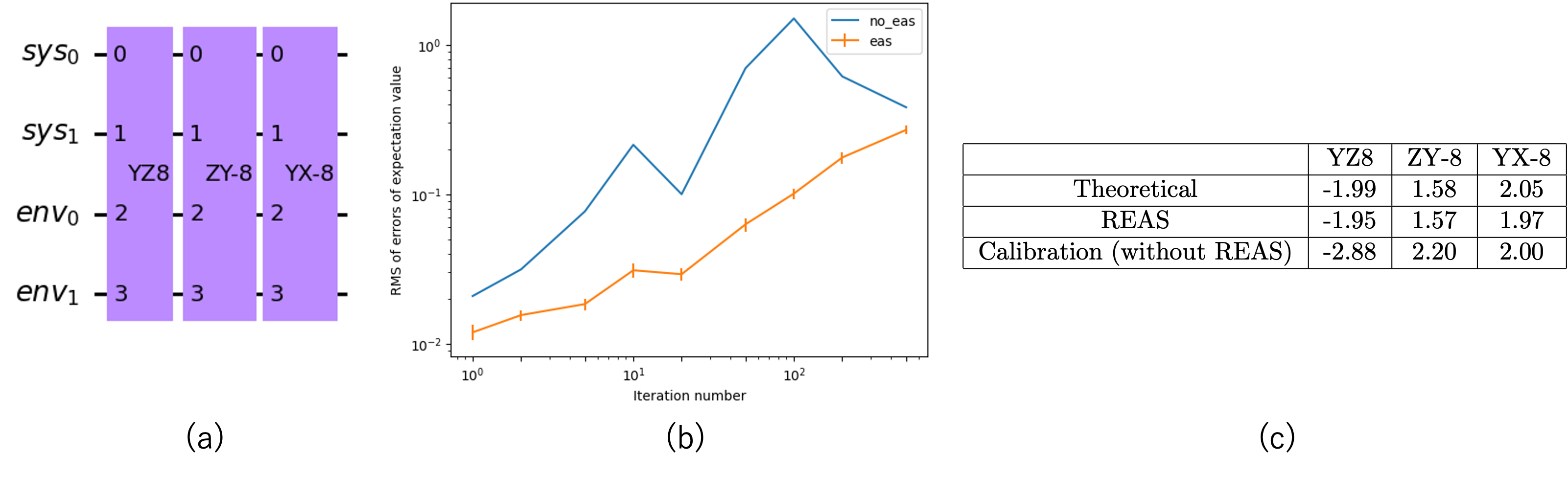
FIG. 1: (a) Repeated circuit.—We consider a deep circuit composed of repeated blocks $YZ8$, $ZY$-$8$, $YZ$-$8$, where, e.g., $YZ8$ corresponds to $e^{-i\frac{\pi}{8}YZ}\otimes I_{\rm env}$ and similar for the others. (b) REAS performance in a deep circuit.—The blocks are iterated a number of times, leading to overall circuits of growing depth, and measure the expectation value of $IZII$. (c) Shift in rotation angle ($10^{-3}$ rad).—Here we calculate the shift in rotation angle, i.e., the coherent error, in theory as well as with REAS and with conventional calibration techniques, highlighting the performance of the former.

The graph in Fig. 1 (b) shows that the scaling of the RMS of the difference in the expectation value is nearly of order $\text{(Iteration number)}^{1/2}$. Although the theory only predicts that the RMS is upper bounded by a function scaling like $\text{(Iteration number)}^{1/2}$, which does not imply that a change in the value of RMS always follows this scaling (e.g., oscillations of the RMS value are possible), the value of the power calculated here is $\approx 0.501$, corresponding closely to the upper bound. In contrast, the corresponding scaling for the case without REAS grows faster (approximately linearly) until it reaches the saturation point. The table in Fig. 1 (c) shows that the value of rotation shift caused by the coherent error is precisely estimated by the REAS calibration with error less than $0.1\times 10^{-3}\ {\rm rad}$. In contrast, the estimate of this rotation shift deviates further from the theoretical prediction when using calibration without REAS. This result implies that the usual calibration based on the phase estimation without inserting random Pauli cannot precisely remove the effect of rotation shift and thus REAS calibration is required.

IV.2 Suppression of the First-order Error

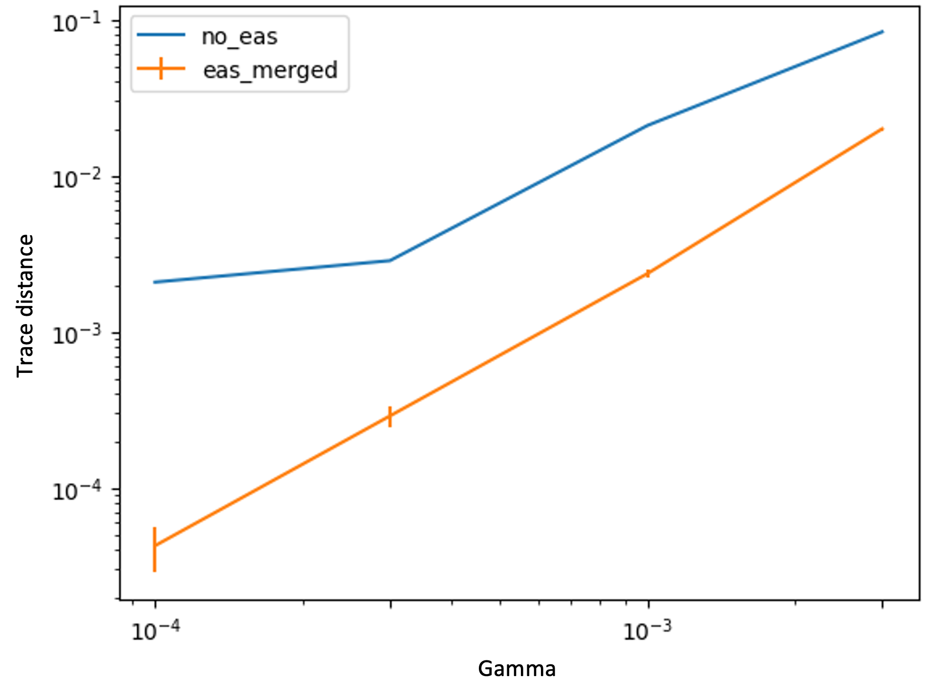
FIG. 2: Suppression of First-order Error.—Here we demonstrate that in the limit $\gamma\to 0$, the first order error term vanishes when REAS is applied, in contrast to the case where it is not, as predicted by theory.

In Fig. 2, we demonstrate that the first-order term of the error vanishes in the regime where $\gamma$ is near zero (i.e., the weak-coupling regime), as predicted by theory. We randomly generate a circuit with a depth of 1000, which only contains two-qubit Pauli rotations. For $\gamma\in\{0.0001,0.0003,0.001,0.003\}$, we compute the average trace distance between the state obtained after running the error-free circuit and that obtained after running a noisy circuit without/with REAS (sampling number: 4000). The simulation in Fig. 2 shows a near quadratic dependence of the trace distance on $\gamma$ when using REAS, whereas the scaling for the case without REAS is near linear for small $\gamma$.

IV.3 Effectiveness of Single Pauli Transformation

In Fig. 3, we demonstrate how incorporating the single Pauli transformation helps to reduce decoherence noise. We randomly generated a circuit with a depth of 1000, which contains both single-qubit and two-qubit Pauli gates. For $\gamma\in\{0.0002,0.0005,0.001,0.005\}$, we then computed the average trace distance between the state obtained after running the ideal circuit and that obtained after running the noisy circuit first without REAS, and then with REAS, both with and without the single Pauli transformation (sampling number: 4000). The simulation shown in Fig. 3 shows that the circuit implemented with the single Pauli transformation included displays a smaller trace distance in the small $\gamma$ regime compared to the case where Pauli rotation is implemented directly without said transformation procedure.

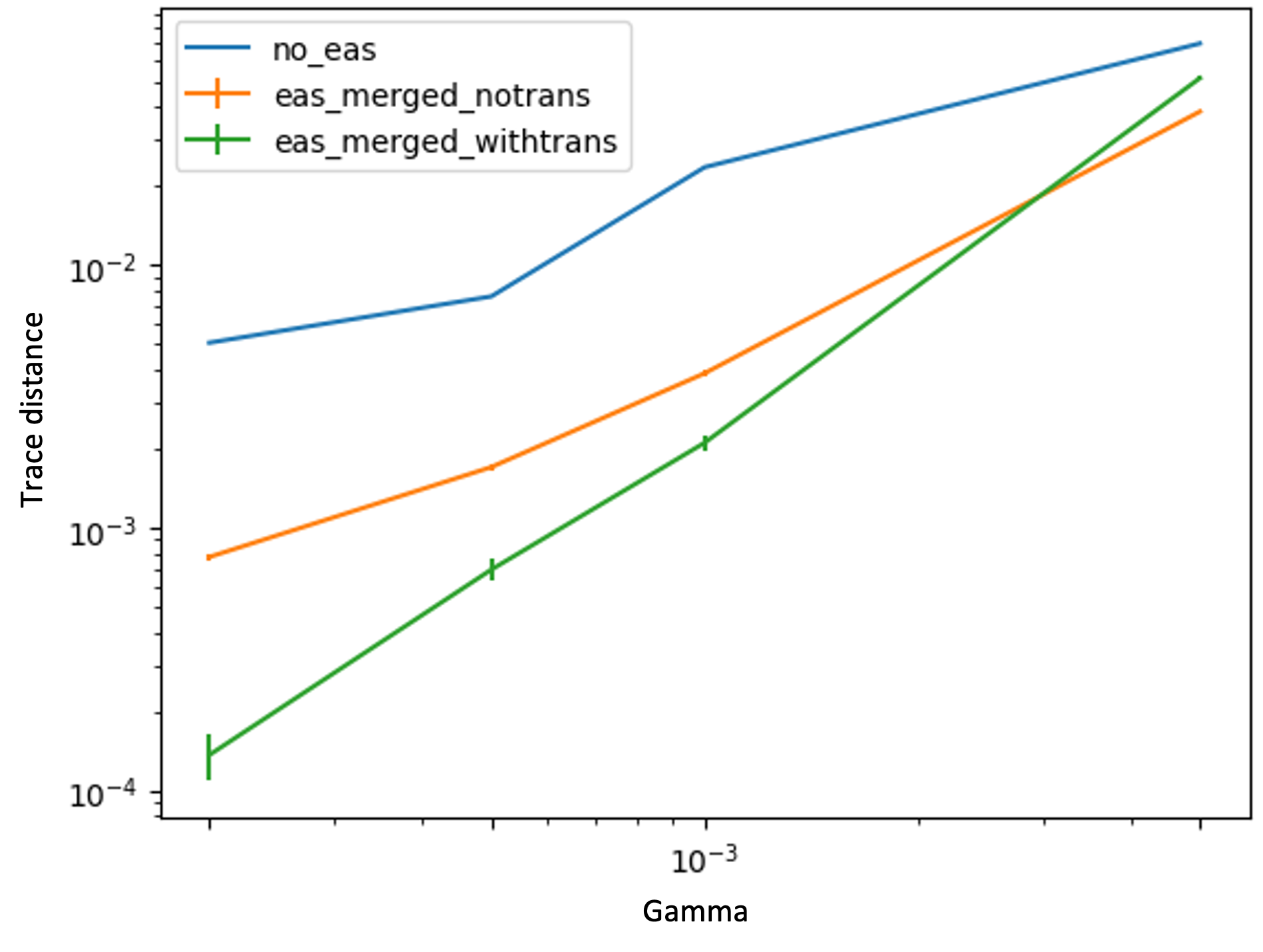
FIG. 3: Effectiveness of Single Pauli Transformation.—Here we demonstrate the suppression of decoherence errors by comparing three situations: first, without REAS (blue); second, with REAS but without incorporating the single Pauli transformation procedure (orange); and third, with REAS and single Pauli transformation (green). The behavior improves accordingly.

V Summary

To summarize, we have presented an advanced, robust method of quantum error suppression. The ability to deal with non-Clifford circuits and incorporate both coherent and decoherence errors, both in the original circuit and in its modification, stems from combining robust phase estimation techniques with a calibrated Pauli twirling-type procedure, as described in Secs. II and III. To highlight the immediate applicability of our results, we present numerical evidence for the quadratic reduction in error growth presented in Sec. IV. Since the types of errors that our method is tailor-made to deal with go far beyond the current state-of-the-art, we expect our methods to be widely adopted across a variety of platforms.

Looking forward, extending our method to deal with leakage/qubit loss will be an important generalization. Secondly, an improved technique of dealing with errors across many qubits, e.g., non-local crosstalk, is required since the performance of our technique suffers in terms of qubit number. Lastly, actively suppressing errors in complex non-Markovian processes remains of utmost importance, especially as the timescales over which one can access quantum systems are ever decreasing, making non-trivial temporal correlations more prevalent [38, 39, 40, 41, 42, 43, 44].

Note

Upon completion of this work, we became aware of a related method that generalizes Pauli twirling techniques to non-Clifford circuits [45].

Appendix A Suppression of Coherent Errors by REAS

Here, we demonstrate how the REAS protocol can deal with coherent errors. For simplicity, suppose that the gate sequence that one wishes to implement in the computation does not involve parallel application of Pauli rotation gates, i.e., it can be written as

$$\prod_{j=1}^{L}e^{-i\sigma_{j}\theta_{j}}\in\mathcal{L}(\mathcal{H})$$ (23)

using single- or two-qubit Pauli operators $\sigma_{1},\ldots,\sigma_{L}$ and rotation angles $\theta_{1},\ldots,\theta_{N}$. Again, we abbreviate the tensor product with the identity on the systems that undergo trivial dynamics. Suppose that coherent errors affect each Pauli rotation $e^{-is\sigma_{j}\theta_{j}}\ (s\in\{+1,-1\})$ so that the actual noisy gate implemented is expressed as $e^{-is\sigma_{j}\theta_{j}}[I+i\epsilon C_{s,j}]$ for some unitary $I+i\epsilon C_{s,j}$ where $\epsilon>0$ and $\|C_{s,j}\|_{\rm op}\leq 1$ for all $(s,j)$. Here, we assume that the same error occurs on the same type of gate at any time, namely, $C_{s,j}=C_{s,k}$ if $(\sigma_{j},\theta_{j})=(\sigma_{k},\theta_{k})$, which is rather natural and required to enable calibration.

Since each $C_{s,j}$ is defined on $\mathcal{H}$, it can be decomposed in terms of a linear combination of $n$-qubit Pauli operators as

$$C_{s,j}=:\sum_{\vec{v}\in\{0,1,2,3\}^{n}}\alpha_{\vec{v},j}(s)\sigma_{\vec{v}}$$ (24)

using complex numbers $\alpha_{\vec{v}}(s)\in\mathbb{C}$. Importantly, note that $\alpha_{\vec{v},j}(s)$ can be further decomposed into a sum of $s$-dependent part and $s$-independent part as $\alpha_{\vec{v},j}(s)=:\overline{\alpha}_{\vec{v},j}+s\Delta\alpha_{\vec{v},j}$, where $\overline{\alpha}_{\vec{v},j}:=\tfrac{1}{2}[\alpha_{\vec{v},j}(1)+\alpha_{\vec{v},j}(-1)]$ and $\Delta{\alpha}_{\vec{v},j}:=\tfrac{1}{2}[\alpha_{\vec{v},j}(1)-\alpha_{\vec{v},j}(-1)]$. We will frequently make use of this technique throughout this analysis.

Since the operator $[I+i\epsilon C_{s,j}]$ is unitary, it follows that

$$\left[I+i\epsilon\sum_{\vec{v}}\alpha_{\vec{v},j}(s)\sigma_{\vec{v}}\right]\left[I-i\epsilon\sum_{\vec{v}}\alpha^{*}_{\vec{v},j}(s)\sigma_{\vec{v}}\right] =I+i\epsilon\left(\sum_{\vec{v}}(\alpha_{\vec{v},j}(s)-\alpha^{*}_{\vec{v},j}(s))\right)+O(\epsilon^{2})=I,$$ (25)

which implies that the 0${}^{\text{th}}$ order $\epsilon$ term $\alpha_{\vec{v},j}^{(0)}$ of $\alpha_{\vec{v},j}$ is real. Moreover, we can take the 0${}^{\text{th}}$ order $\epsilon$ term $\alpha_{\vec{0},j}$, namely $\alpha_{\vec{0},j}^{(0)}$, the dominant term of the coefficient of $I$, to be $0$ without loss of generality. This is because it can be canceled via an appropriate global phase, as follows

$$\frac{1-i\epsilon\alpha_{\vec{0},j}^{(0)}}{\sqrt{1+(\epsilon\alpha_{\vec{0},j}^{(0)})^{2}}}\left[I+i\epsilon\sum_{\vec{v}}(\alpha_{\vec{v},j}^{(0)}(s)+O(\epsilon))\sigma_{\vec{v}}\right] =\frac{1}{\sqrt{1+(\epsilon\alpha_{\vec{0},j}^{(0)})^{2}}}\left[I+i\epsilon\left\{O(\epsilon)I+\sum_{\vec{v}\neq\vec{0}}\left(\alpha_{\vec{v},j}^{(0)}(s)+O(\epsilon)\right)\sigma_{\vec{v}}\right\}\right]$$

$$=(1-O(\epsilon^{2}))\left[I+i\epsilon\left\{O(\epsilon)I+\sum_{\vec{v}\neq\vec{0}}\left(\alpha_{\vec{v},j}^{(0)}(s)+O(\epsilon)\right)\sigma_{\vec{v}}\right\}\right]$$

$$=:I+i\epsilon\sum_{\vec{v}\neq\vec{0}}{\alpha}_{\vec{v},j}^{(0)}(s)\sigma_{\vec{v}}+O(\epsilon^{2}).$$ (26)

Thus, we assume that $C_{s,j}$ is defined such that $\alpha_{\vec{0},j}^{(0)}(s)=0$ for all $(s,j)$.

Now, we move on to the error analysis of the gate sequence obtained by inserting random Pauli gates via REAS into Eq. (23). This leads to

$$\sigma_{\vec{v}_{L}}e^{-is_{L}\sigma_{L}\theta_{L}}\prod_{j=1}^{L-1}\left[\sigma_{\vec{v}_{j+1:j}}e^{-is_{j}\sigma_{j}\theta_{j}}\right]\sigma_{\vec{v}_{1}},$$ (27)

where $\vec{v}_{1},\ldots,\vec{v}_{L}$ are uniformly randomly chosen vectors. For simplicity, here we have assumed that a random Pauli gate is inserted between all single Pauli rotation gates. Recall that $s_{j}\in\{+1,-1\}$ is defined as

$$s_{j}:=\begin{cases}1&(\sigma_{j}\text{ and }\sigma_{\vec{v}_{j}}\text{ commutes})\\ -1&(\sigma_{j}\text{ and }\sigma_{\vec{v}_{j}}\text{ anti-commutes})\\ \end{cases}.$$ (28)

When such a gate sequence is applied on an arbitrary input state $\rho\in\mathcal{L}(\mathcal{H})$, the result is

$$\left(\frac{1}{4^{n}}\right)^{L}\sum_{\vec{v}_{1},\ldots,\vec{v}_{L}}\left[\sigma_{\vec{v}_{L}}e^{-is_{L}\sigma_{L}\theta_{L}}\overleftarrow{\prod_{j=1}^{L-1}}\left[\sigma_{\vec{v}_{j+1:j}}e^{-is_{j}\sigma_{j}\theta_{j}}\right]\sigma_{\vec{v}_{1}}\right]\rho\left[\sigma_{\vec{v}_{1}}\overrightarrow{\prod_{j=1}^{L-1}}\left[e^{is_{j}\sigma_{j}\theta_{j}}\sigma_{\vec{v}_{j+1:j}}\right]e^{is_{L}\sigma_{L}\theta_{L}}\sigma_{\vec{v}_{L}}\right]$$

$$= \left(\frac{1}{4^{n}}\right)^{L}\sum_{\vec{v}_{1},\ldots,\vec{v}_{L}}\left[\sigma_{\vec{v}_{L}}e^{-is_{L}\sigma_{L}\theta_{L}}\overleftarrow{\prod_{j=1}^{L-1}}\left[\sigma_{\vec{v}_{j+1}}\sigma_{\vec{v}_{j}}e^{-is_{j}\sigma_{j}\theta_{j}}\right]\sigma_{\vec{v}_{1}}\right]\rho\left[\sigma_{\vec{v}_{1}}\overrightarrow{\prod_{j=1}^{L-1}}\left[e^{is_{j}\sigma_{j}\theta_{j}}\sigma_{\vec{v}_{j}}\sigma_{\vec{v}_{j+1}}\right]e^{is_{L}\sigma_{L}\theta_{L}}\sigma_{\vec{v}_{L}}\right].$$ (29)

Here, we use notation $\overleftarrow{\prod}$ and $\overrightarrow{\prod}$ to distinguish the order of applying the gate sequences, defined such that

$$\overleftarrow{\prod_{j=1}^{L}}M_{j}=M_{L}\cdots M_{1}\quad\quad\quad\quad\text{and}\quad\quad\quad\quad\overrightarrow{\prod_{j=1}^{L}}M_{j}=M_{1}\cdots M_{L}$$ (30)

for linear operators $M_{1},\ldots,M_{L}$. It is straightforward to verify that when no error terms appears, Eq. (A) reduces to the ideal state transformation

$$\left(\overleftarrow{\prod_{j=1}^{L}}e^{-i\sigma_{j}\theta_{j}}\right)\rho\left(\overrightarrow{\prod_{j=1}^{L}}e^{i\sigma_{j}\theta_{j}}\right),$$ (31)

which can be seen by moving the inner Pauli operators $\sigma_{\vec{v}_{j}}$ outward, making them pass through $e^{\pm is_{j}\sigma_{j}\theta_{j}}$ and thereby changing $e^{\pm is_{j}\sigma_{j}\theta_{j}}$ to $e^{\pm i\sigma_{j}\theta_{j}}$, and subsequently canceling with the corresponding outer $\sigma_{\vec{v}_{j}}$ operator.

We now prove that, as claimed in the main text, coherent errors lead to Eq. (A) being transformed as

$$\left(\overleftarrow{\prod_{j=1}^{L}}e^{-i\sigma_{j}(\theta_{j}-\epsilon\Delta\theta_{j})}\right)\rho\left(\overrightarrow{\prod_{j=1}^{L}}e^{i\sigma_{j}(\theta_{j}-\epsilon\Delta\theta_{j})}\right)+O(\epsilon+\epsilon^{2}L),$$ (32)

where $\epsilon\Delta\theta_{j}:=\tan^{-1}(\epsilon\Delta\alpha_{\vec{w}_{j},j}^{(0)})$ where $\sigma_{\vec{w}_{j}}:=\sigma_{j}$. Our technique of erasing errors is based on the following equations regarding averaging over an $n$-qubit Pauli operator $\sigma$

$$\left(\frac{1}{4^{n}}\right)\sum_{\vec{v}\in\{0,1,2,3\}^{n}}\sigma_{\vec{v}}\sigma\sigma_{\vec{v}}=\begin{cases}I&\quad\quad\text{for }\sigma=I\\ 0&\quad\quad\text{for }\sigma\neq I\end{cases}$$ (33)

and

$$\left(\frac{1}{4^{n}}\right)\sum_{\vec{v}\in\{0,1,2,3\}^{n}}\sigma_{\vec{v}}s(\sigma_{\vec{v}},\sigma^{\prime})\sigma\sigma_{\vec{v}}=\begin{cases}\sigma^{\prime}&\quad\quad\text{for }\sigma=\sigma^{\prime}\\ 0&\quad\quad\text{for }\sigma\neq\sigma^{\prime}\end{cases}$$ (34)

where $s(\sigma_{\vec{v}},\sigma^{\prime})$ is defined as

$$s(\sigma_{\vec{v}},\sigma^{\prime}):=\begin{cases}1&(\sigma_{\vec{v}}\text{ and }\sigma^{\prime}\text{ commutes})\\ -1&(\sigma_{\vec{v}}\text{ and }\sigma^{\prime}\text{ ant-commutes})\end{cases}.$$ (35)

With this, the error term $i\epsilon C_{s_{j^{\prime}},j^{\prime}}$ transforms as

$$\frac{1}{4^{n}}\sum_{\vec{v}_{j^{\prime}}}\sigma_{\vec{v}_{j^{\prime}}}i\epsilon C_{s_{j^{\prime}},j^{\prime}}\sigma_{\vec{v}_{j^{\prime}}}=\frac{1}{4^{n}}\sum_{\vec{v}_{j^{\prime}}}\sigma_{\vec{v}_{j^{\prime}}}\left[\sum_{\vec{u}}i\epsilon(\overline{\alpha}_{\vec{u},j^{\prime}}+s_{j^{\prime}}\Delta\alpha_{\vec{u},j^{\prime}})\sigma_{\vec{u}}\right]\sigma_{\vec{v}_{j^{\prime}}}=O(\epsilon^{2})I+i\epsilon\Delta\alpha_{\vec{w}_{j^{\prime}},j^{\prime}}\sigma_{j^{\prime}}$$ (36)

where $\sigma_{\vec{w}_{j^{\prime}}}=\sigma_{j^{\prime}}$ by definition. This expression can be simplified by absorbing the first-order $\epsilon$ part in $i\epsilon s_{j^{\prime}}\Delta\alpha_{\vec{w}_{j^{\prime}},j^{\prime}}\sigma_{j^{\prime}}$ to a shift in the rotation angle of $e^{-is_{j^{\prime}}\sigma_{j^{\prime}}\theta_{j^{\prime}}}$ as follows

$$e^{-is_{j^{\prime}}\sigma_{j^{\prime}}\theta_{j^{\prime}}}[I+i\epsilon C_{s_{j^{\prime}},j^{\prime}}] =:g\left(e^{-is_{j^{\prime}}\sigma_{j^{\prime}}\theta_{j^{\prime}}}\right)$$

$$=e^{-is_{j^{\prime}}\sigma_{j^{\prime}}\theta_{j^{\prime}}}e^{i\epsilon s_{j^{\prime}}\Delta\theta_{j^{\prime}}\sigma_{j^{\prime}}}\frac{1-is_{j^{\prime}}\epsilon\Delta\alpha_{\vec{w}_{j^{\prime}},j^{\prime}}^{(0)}}{\sqrt{1+(\epsilon\Delta\alpha_{\vec{w}_{j^{\prime}},j^{\prime}}^{(0)})^{2}}}\left[I+i\epsilon\sum_{\vec{u}\neq\vec{0}}(\overline{\alpha}_{\vec{u},j^{\prime}}+s_{j^{\prime}}\Delta\alpha_{\vec{u},j^{\prime}})\sigma_{\vec{u}}+O(\epsilon^{2})\right]$$

$$=e^{-is_{j^{\prime}}\sigma_{j^{\prime}}(\theta_{j^{\prime}}-\epsilon\Delta\theta_{j^{\prime}})}\left[1-O(\epsilon^{2})\right]\left[I+i\epsilon\sum_{\vec{u}\notin\{\vec{0},\vec{w}_{j^{\prime}}\}}(\overline{\alpha}_{\vec{u},j^{\prime}}+s_{j^{\prime}}\Delta\alpha_{\vec{u},j^{\prime}})\sigma_{\vec{u}}+i\epsilon\overline{\alpha}_{\vec{w}_{j^{\prime}},j^{\prime}}\sigma_{j^{\prime}}+O(\epsilon^{2})\right]$$

$$=e^{-is_{j^{\prime}}\sigma_{j^{\prime}}(\theta_{j^{\prime}}-\epsilon\Delta\theta_{j^{\prime}})}\left[I+i\epsilon\sum_{\vec{u}\notin\{\vec{0},\vec{w}_{j^{\prime}}\}}(\overline{\alpha}_{\vec{u},j^{\prime}}+s_{j^{\prime}}\Delta\alpha_{\vec{u},j^{\prime}})\sigma_{\vec{u}}+i\epsilon\overline{\alpha}_{\vec{w}_{j^{\prime}},j^{\prime}}\sigma_{j^{\prime}}+O(\epsilon^{2})\right]$$

$$=:e^{-is_{j^{\prime}}\sigma_{j^{\prime}}(\theta_{j^{\prime}}-\epsilon\Delta\theta_{j^{\prime}})}[I+i\epsilon D_{s_{j^{\prime}},j^{\prime}}]=:g^{\prime}\left(e^{-is_{j^{\prime}}\sigma_{j^{\prime}}(\theta_{j^{\prime}}-\epsilon\Delta\theta_{j^{\prime}})}\right).$$ (37)

Thus, the error term $i\epsilon D_{s_{j^{\prime}},j^{\prime}}$ no longer contains the first-order $\epsilon$ term proportional to $s_{j^{\prime}}\sigma_{{j^{\prime}}}$. Using this result, Eq. (A) with coherent errors can be rewritten as

$$\left(\frac{1}{4^{n}}\right)^{L}\sum_{\vec{v}_{1},\ldots,\vec{v}_{L}}\left[g(\sigma_{\vec{v}_{L}})g(e^{-is_{L}\sigma_{L}\theta_{L}})\overleftarrow{\prod_{j=1}^{L-1}}\left[g(\sigma_{\vec{v}_{j+1:j}})g(e^{-is_{j}\sigma_{j}\theta_{j}})\right]g(\sigma_{\vec{v}_{1}})\right]\rho\left[\cdots\right]$$

$$= \left(\frac{1}{4^{n}}\right)^{L}\sum_{\vec{v}_{1},\ldots,\vec{v}_{L}}\left[g(\sigma_{\vec{v}_{L}})g^{\prime}(e^{-is_{L}\sigma_{L}(\theta_{L}-\epsilon\Delta\theta_{L})})\overleftarrow{\prod_{j=1}^{L-1}}\left[g(\sigma_{\vec{v}_{j+1:j}})g^{\prime}(e^{-is_{j}\sigma_{j}(\theta_{j}-\Delta\theta_{j})})\right]g(\sigma_{\vec{v}_{1}})\right]\rho\left[\cdots\right]$$ (38)

where the error function $g$ on inserted random Pauli operators $\sigma_{\vec{v}}$ is defined as $g(\sigma_{\vec{v}})=:\sigma_{\vec{v}}[i+i\epsilon\widetilde{C}_{\vec{v}}]$ such that $i\epsilon\widetilde{C}_{\vec{v}}$ has no $O(\epsilon)$ term proportional to $I$. Here, the notation [$\ldots$] on the right of $\rho$ represents the Hermitian conjugate of the corresponding product on the left; we will continue to use similar notation below.

We move to analyze the suppression of errors. Consider a single error term on a particular Pauli rotation gate $e^{-is_{j^{\prime}}\sigma_{j^{\prime}}\theta_{j^{\prime}}}$ in the computation, which leads to an expression of the form

$$\left(\frac{1}{4^{n}}\right)^{L}\sum_{\vec{v}_{1},\ldots,\vec{v}_{L}}\left[\sigma_{\vec{v}_{L}}[\cdots]\sigma_{\vec{v}_{j^{\prime}+1,j^{\prime}}}(e^{-is_{j^{\prime}}\sigma_{j^{\prime}}(\theta_{j^{\prime}}-\epsilon\Delta\theta_{j^{\prime}})}i\epsilon D_{s_{j^{\prime}},j^{\prime}})\sigma_{\vec{v}_{j^{\prime}-1:j^{\prime}}}[\cdots]\sigma_{\vec{v}_{1}}\right]\rho\left[\sigma_{\vec{v}_{1}}[\cdots]\sigma_{\vec{v}_{L}}\right]$$

$$= \left(\frac{1}{4^{n}}\right)^{L}\sum_{\vec{v}_{1},\ldots,\vec{v}_{L}}\left[\sigma_{\vec{v}_{L}}[\cdots]\sigma_{\vec{v}_{j^{\prime}+1}}\sigma_{\vec{v}_{j^{\prime}}}(e^{-is_{j^{\prime}}\sigma_{j^{\prime}}(\theta_{j^{\prime}}-\epsilon\Delta\theta_{j^{\prime}})}i\epsilon D_{s_{j^{\prime}},j^{\prime}})\sigma_{\vec{v}_{j^{\prime}}}\sigma_{\vec{v}_{j^{\prime}-1}}[\cdots]\sigma_{\vec{v}_{1}}\right]\rho\left[\sigma_{\vec{v}_{1}}[\cdots]\sigma_{\vec{v}_{L}}\right].$$ (39)

All pairs of inserted Pauli operators $\sigma_{\vec{v}_{j}}$ other than $\sigma_{\vec{v}_{j^{\prime}}}$ that sandwich $i\epsilon D_{s_{j^{\prime}},j^{\prime}}$ can pass through the operator $e^{\pm is_{j}\sigma_{j}(\theta_{j}-\epsilon\Delta\theta_{j})}$ and cancel with each other. Thus, Eq. (A) can be rewritten as

$$\frac{1}{4}\sum_{\vec{v}_{j^{\prime}}}\left[\left(\overleftarrow{\prod_{j=j^{\prime}+1}^{L}}e^{-i\sigma_{j}(\theta_{j}-\epsilon\Delta\theta_{j})}\right)\sigma_{\vec{v}_{j^{\prime}}}e^{-is_{j^{\prime}}\sigma_{j^{\prime}}(\theta_{j^{\prime}}-\epsilon\Delta\theta_{j^{\prime}})}i\epsilon D_{s_{j^{\prime}},j^{\prime}}\sigma_{\vec{v}_{j^{\prime}}}\left(\overleftarrow{\prod_{j=1}^{j^{\prime}-1}}e^{-i\sigma_{j}(\theta_{j}-\epsilon\Delta\theta_{j})}\right)\right]\rho\left[\overrightarrow{\prod_{j=1}^{L}}e^{is_{j}\sigma_{j}(\theta_{j}-\epsilon\Delta\theta_{j})}\right]$$

$$= \left[\left(\overleftarrow{\prod_{j=j^{\prime}+1}^{L}}e^{-i\sigma_{j}\theta_{j}}\right)e^{-i\sigma_{j^{\prime}}(\theta_{j^{\prime}}-\epsilon\Delta\theta_{j^{\prime}})}\left(\frac{1}{4^{n}}\sum_{\vec{v}_{j^{\prime}}}\sigma_{\vec{v}_{j^{\prime}}}i\epsilon D_{s_{j^{\prime}},j^{\prime}}\sigma_{\vec{v}_{j^{\prime}}}\right)\left(\overleftarrow{\prod_{j=1}^{j^{\prime}-1}}e^{-i\sigma_{j}(\theta_{j}-\epsilon\Delta\theta_{j})}\right)\right]\rho\left[\overrightarrow{\prod_{j=1}^{L}}e^{is_{j}\sigma_{j}(\theta_{j}-\epsilon\Delta\theta_{j})}\right]$$

$$= \left[\left(\overleftarrow{\prod_{j=j^{\prime}+1}^{L}}e^{-i\sigma_{j}\theta_{j}}\right)e^{-i\sigma_{j^{\prime}}(\theta_{j^{\prime}}-\epsilon\Delta\theta_{j^{\prime}})}\left(O(\epsilon^{2})I+O(\epsilon^{2})\sigma_{\vec{w}_{j^{\prime}}}\right)\left(\overleftarrow{\prod_{j=1}^{j^{\prime}-1}}e^{-i\sigma_{j}(\theta_{j}-\epsilon\Delta\theta_{j})}\right)\right]\rho\left[\overrightarrow{\prod_{j=1}^{L}}e^{is_{j}\sigma_{j}(\theta_{j}-\epsilon\Delta\theta_{j})}\right]$$

$$= \,O(\epsilon^{2}).$$ (40)

Next, we consider the case where a single error term in Eq. (A) occurs on one of the inserted Pauli operators $\sigma_{\vec{v}_{j^{\prime}+1:j^{\prime}}}$. This leads to Eq. (A) being expressed as

$$\left(\frac{1}{4^{n}}\right)^{L}\sum_{\vec{v}_{1},\ldots,\vec{v}_{L}}\left[\sigma_{\vec{v}_{L}}[\cdots]\sigma_{\vec{v}_{j^{\prime}+2,j^{\prime}+1}}e^{-is_{j^{\prime}+1}\sigma_{j^{\prime}+1}(\theta_{j^{\prime}+1}-\epsilon\Delta\theta_{j^{\prime}+1})}(\sigma_{\vec{v}_{j^{\prime}+1:j^{\prime}}}i\epsilon\widetilde{C}_{\vec{v}_{j^{\prime}+1:j^{\prime}}})e^{-is_{j^{\prime}}\sigma_{j^{\prime}}(\theta_{j^{\prime}}-\epsilon\Delta\theta_{j^{\prime}})}\sigma_{\vec{v}_{j^{\prime}:j^{\prime}-1}}[\cdots]\sigma_{\vec{v}_{1}}\right]\rho[\cdots]$$

$$= \left(\frac{1}{4^{n}}\right)^{L}\sum_{\vec{v}_{1},\ldots,\vec{v}_{L}}\left[\sigma_{\vec{v}_{L}}[\cdots]\sigma_{\vec{v}_{j^{\prime}+2}}\sigma_{\vec{v}_{j^{\prime}+1}}e^{-is_{j^{\prime}+1}\sigma_{j^{\prime}+1}(\theta_{j^{\prime}+1}-\epsilon\Delta\theta_{j^{\prime}+1})}(\sigma_{\vec{v}_{j^{\prime}+1}}\sigma_{\vec{v}_{j^{\prime}}}i\epsilon\widetilde{C}_{\vec{v}_{j^{\prime}+1:j^{\prime}}})e^{-is_{j^{\prime}}\sigma_{j^{\prime}}(\theta_{j^{\prime}}-\epsilon\Delta\theta_{j^{\prime}})}\sigma_{\vec{v}_{j^{\prime}}}\sigma_{\vec{v}_{j^{\prime}-1}}[\cdots]\sigma_{\vec{v}_{1}}\right]\rho[\cdots]$$

$$= \left(\frac{1}{4^{n}}\right)^{2}\sum_{\vec{v}_{j^{\prime}+1},\vec{v}_{j^{\prime}}}\left(\prod_{j=j^{\prime}+1}^{L}e^{-i\sigma_{j}(\theta_{j}-\epsilon\Delta\theta_{j})}\right)\sigma_{\vec{v}_{j^{\prime}}}i\epsilon\widetilde{C}_{\vec{v}_{j^{\prime}+1:j^{\prime}}}\sigma_{\vec{v}_{j^{\prime}}}\left(\prod_{j=1}^{j^{\prime}}e^{-i\sigma_{j}(\theta_{j}-\epsilon\Delta\theta_{j})}\right)\rho[\cdots]$$

$$= \left(\prod_{j=j^{\prime}+1}^{L}e^{-i\sigma_{j}(\theta_{j}-\epsilon\Delta\theta_{j})}\right)\left\{\frac{1}{4^{n}}\sum_{\vec{v}_{j^{\prime}}}\sigma_{\vec{v}_{j^{\prime}}}\left(\frac{1}{4^{n}}\sum_{\vec{v}_{j^{\prime}+1}}\widetilde{C}_{\vec{v}_{j^{\prime}+1:j^{\prime}}}\right)\sigma_{\vec{v}_{j^{\prime}}}\right\}\left(\prod_{j=1}^{j^{\prime}}e^{-i\sigma_{j}(\theta_{j}-\epsilon\Delta\theta_{j})}\right)\rho[\cdots],$$ (41)

which is also $O(\epsilon^{2})$ since $\sum_{\vec{v}_{j^{\prime}+1}}\widetilde{C}_{\vec{v}_{j^{\prime}+1:j^{\prime}}}=\sum_{\vec{u}}\widetilde{C}_{\vec{u}}$ is independent of $\vec{v}_{j^{\prime}}$ and has only $O(\epsilon^{2})$ term proportional to $I$.

Finally, let us consider how many first- and second-order $\epsilon$ terms can possibly appear in Eq. (A). The first-order $\epsilon$ terms can only appear in the expansion of Eq. (A) when a single error term is chosen at either $\sigma_{\vec{v}_{1}}$ or $\sigma_{\vec{v}_{L}}$. Thus, the first-order $\epsilon$ terms in Eq. (A) do not scale in terms of $L$ and behave like $O(\epsilon)$. The second-order $\epsilon$ terms can originate from any term in the expansion of Eq. (A) where a single error term occurs at a single Pauli rotation in the computation $e^{\pm is_{j}\sigma_{j}(\theta_{j}-\epsilon\Delta\theta_{j})}$ or at an inserted Pauli operator $\sigma_{\vec{v}_{j:j+1}}$; the sum of such terms is $O(\epsilon^{2}L)$. Technically speaking, a second-order $\epsilon$ term can also possibly appear when two error terms occur in Eq. (A), but for such cases to have a second-order $\epsilon$ term, the errors must appear in close locations; this means that such cases are largely irrelevant in practice. For example, when the error occurs at $e^{\pm is_{j}\sigma_{j}(\theta_{j}-\epsilon\Delta\theta_{j})}$ and $\sigma_{\vec{v}_{k:k+1}}$ with either $j-k\geq 2$ or $k-j\geq 1$, it can be easily shown that the error terms are averaged over random Pauli operators and therefore no more second-order $\epsilon^{2}$ terms remains. Thus, the total sum of these terms in the expansion of Eq. (A) will also be $O(\epsilon^{2}L)$.

In general, $\epsilon^{n}$ terms in Eq. (A) can be shown to be $O(\epsilon^{n}L^{\lfloor\tfrac{n}{2}\rfloor})$, where $\lfloor a\rfloor$ denotes the largest integer not exceeding $a$. This follows from the fact that the first-order $\epsilon$ term in the error can remain only if there exists another error term in a nearby gate. Using this fact, the claim made in Eq. (32) is shown. ∎

Appendix B Root Mean Squared Error Bounds

To obtain an upper bound of the RMS of the error of expectation values in terms of an arbitrary observable $M$, the following statement can be used.

Lemma 1.

For an arbitrary unitary operation defined by $\mathcal{U}(\rho):=U\rho U^{\dagger}$ with a unitary operator $U$ and a density operator $\rho$ on a Hilbert space $\mathcal{H}$, if a set of deterministic quantum operations (completely-positive trace-preserving maps) $\mathcal{F}_{j}:\mathcal{L}(\mathcal{H})\to\mathcal{L}(\mathcal{H})$ and a probability distribution $\{p_{j}\}$ satisfies

$$\|\mathcal{U}-\sum_{j}p_{j}\mathcal{F}_{j}\|_{\diamond}\leq\Delta$$

for some $\Delta>0$, the variance of the averaged operation $\sum_{j}p_{j}\mathcal{F}_{j}$ is upper bounded by

$$\underset{\begin{subarray}{c}\mathrm{dim}(\mathcal{H}^{\prime})\\ \ket{\psi};\|\ket{\psi}\|=1\end{subarray}}{\mathrm{sup}}\sum_{j}p_{j}\|\mathcal{U}\otimes\mathcal{I}(\ket{\psi}\bra{\psi})-\mathcal{F}_{j}\otimes\mathcal{I}(\ket{\psi}\bra{\psi})\|_{1}^{2}\leq 2\Delta,$$ (42)

where $\mathcal{I}$ is the identity operation on a Hilbert space $\mathcal{H}^{\prime}$ and $\ket{\psi}$ is a pure state on $\mathcal{H}\otimes\mathcal{H}^{\prime}$.

The proof is given in App. B of Ref. [46]. For our case, $U$ is the error-free unitary that one desires to implement, $j:=(\vec{v}_{1},\ldots,\vec{v}_{N})$ is the tuple of all random vectors chosen in the REAS scheme, and $p_{j}$ and $\mathcal{F}_{j}$ are the probability that $j$ and the quantum operation on $\mathcal{H}$ which is applied on the state (including the final partial trace of $\mathcal{H}_{\rm env}$) when $j$ is chosen, respectively.

Consider $\mathcal{E}_{\rm shifted}$ to correspond to a gate implemented with a shift in the rotation angle, i.e., the r.h.s. of Eq. (II.2). Since the result regarding such coherent errors implies that $\|\mathcal{E}_{\rm shifted}-\mathcal{E}^{\prime}\|_{\diamond}=C(\epsilon+N\epsilon^{2})$ for constant $C>0$ and $\mathcal{E}^{\prime}=\sum_{j}p_{j}\mathcal{F}_{j}$, where $p_{j}:=(1/4)^{nN}$ and $\mathcal{F}_{j}(\rho):={\rm tr}_{\rm env}[\mathcal{E}^{\prime}_{j}(\rho\otimes\rho_{\rm env})]$, Lem. 1 leads to the following.

Corollary 1.

For an arbitrary observable $A$ on $\mathcal{H}$ such that $\|A\|_{\rm op}\leq 1$, the following equation holds:

$$\underset{\begin{subarray}{c}\ket{\psi};\|\ket{\psi}\|=1\end{subarray}}{\mathrm{sup}}\sum_{j}p_{j}[{\rm tr}\{A\mathcal{E}_{\rm shifted}(\ket{\psi}\bra{\psi})\}-{\rm tr}\{A\mathcal{F}_{j}(\ket{\psi}\bra{\psi})\}]^{2}\leq 2C(\epsilon+N\epsilon^{2})$$ (43)

where $j:=(\vec{v}_{1},\ldots,\vec{v}_{N})$, $p_{j}=(1/4)^{nN}$, and $\mathcal{F}_{j}(\rho):={\rm tr}_{\rm env}[\mathcal{E}^{\prime}_{j}(\rho\otimes\rho_{\rm env})]$.

This means that the RMS of the difference between the error of expectation value is bounded above by $\sqrt{2C(\epsilon+N\epsilon^{2})}$ which approaches to $\sqrt{2C}\epsilon\sqrt{N}$ in the regime $N\gg 1/\epsilon$.

Appendix C Class of Decoherence Errors that can be Suppressed

We now move to demonstrate the more general class of decoherence errors that can be suppressed when our REAS method is supplemented by the single Pauli transformation introduced in Sec. III.2. Specifically, we show that this protocol can suppress errors that are first-order in $\epsilon$ for a particular class of open system-environment dynamics, which includes depolarizing, amplitude-damping, and decoherence models. We assume that the interaction Hamiltonian involves at most two-body interactions.

In attempting to extend the error-suppressing method for the case of coherent errors to the open setting of decoherence, one immediately runs into problem that some errors terms on the computational Pauli gates $e^{-is_{j}\sigma_{j}\theta_{j}}$ cannot be dealt with. In particular, any term of the form $s_{j}\sigma_{j}\otimes M_{\rm env}$, where $M_{\rm env}\neq I_{\rm env}\in\mathcal{H}_{\rm env}$, cannot be absorbed into the shift of the rotation angle $\theta_{j}$, since $\sigma_{j}$ is coupled with $M_{\rm env}$, and therefore cannot be erased by averaging over random inserted Pauli operators as in Eqs. (33) and (34). This inability to suppress such terms can introduce unwanted $O(\epsilon L)$ errors in Eq. (32), since such first-order $\epsilon$ terms can appear in all Pauli computation gates throughout the circuit.

We circumvent this issue by modifying the computational gate sequence implementing $e^{-is_{j}\sigma_{j}\theta_{j}}$ in such a way that the error terms proportional to $s_{j}\sigma_{j}\otimes M_{\rm env}$ for $M_{\rm env}\neq I$ is at most $O(\epsilon^{2})$. This single Pauli transformation consists of decomposing any $e^{-is\sigma\theta}$ into (a) a two-qubit Pauli gate dependent on the rotation direction $s\in\{+1,-1\}$ and (b) another Pauli gate (which can be either a one- or two-qubit Pauli gate) that is independent of $s$. Intuitively, the trick works to suppress error terms that are first-order in $\epsilon$ since these only appear when an error occurs on a single gate in the computation $e^{-is_{j}\sigma_{j}\theta_{j}}$ and: (a) the $s$-dependent two-qubit Pauli gate does not produce harmful first-order $\epsilon$ terms; and (b) the other $s$-independent Pauli gate does not produce any error term that depends upon $s$.

First, we show that any gate $e^{-is\sigma_{\vec{v}_{0}}\theta}$ corresponding to a two-qubit Pauli operator involves only $O(\epsilon^{2})$ terms proportional to $s\sigma_{\vec{v}_{0}}\otimes M_{\rm env}$ for $M_{\rm env}\neq I$. Note that we always take the Hamiltonian to be traceless without loss of generality (since any trace part only contributes to a global phase).

Lemma 2.

Consider a time interval $t\in[0,T]$, any two-qubit Pauli operator $\sigma_{\vec{v}_{0}}\in\mathcal{L}(\mathcal{H})$, a time-dependent interaction Hamiltonian $\epsilon H^{\prime}(t)\in\mathcal{L}(\mathcal{H}\otimes\mathcal{H}_{\rm env})$ which contains at most two-body terms and has operator norm $O(\epsilon)$, a background Hamiltonian $H_{\rm env}$ of the environment, and a function $\Omega(t)$ such that $\int_{0}^{T}{\rm d}\,\tau\Omega(\tau)=\theta$. In this setting, the total Hamiltonian $s\Omega(t)\sigma_{\vec{v}_{0}}\otimes I_{\rm env}+I\otimes H_{\rm env}+\epsilon H^{\prime}(t)$ gives rise to the unitary operator

$$\mathcal{T}\exp\left[-i\int_{0}^{t}{\rm d}\tau(s\Omega(t)\sigma_{\vec{v}_{0}}\otimes I_{\rm env}+I\otimes H_{\rm env}+\epsilon H^{\prime}(t))\right]=: \left(e^{-is\sigma_{\vec{v}_{0}}\theta}\otimes e^{-iH_{\rm env}T}\right)\left[I+i\epsilon C_{\vec{v}_{0}}\right]$$

$$=: \left(e^{-is\sigma_{\vec{v}_{0}}\theta}\otimes e^{-iH_{\rm env}T}\right)\left[I+i\epsilon\sum_{\vec{w}\in\{0,1,2,3\}^{n}}\sigma_{\vec{w}}\otimes D_{\vec{v}_{0};\vec{w}}(s)\right],$$ (44)

where $\epsilon D_{\vec{v}_{0};\vec{v}_{0}}(s)=\epsilon\alpha I+O(\epsilon^{2})$ for some $\alpha$.

Note that the assumption that the operator norm of the interaction Hamiltonian is $O(\epsilon)$ is consistent with the assumption that the error term $C_{\vec{v}_{0}}$ has operator norm of the same order.

Proof:  For general time-dependent Hamiltonians $H_{1}(t)$ and $H_{2}(t)$, the Hamiltonian dynamics generated by $H_{1}+H_{2}$ can be written as

$$\mathcal{T}\exp\left[-i\int_{0}^{t}{\rm d}\tau\{H_{1}(\tau)+H_{2}(\tau)\}\right]=U_{1}(t)\mathcal{T}\exp\left[-i\int_{0}^{t}{\rm d}\tau U_{1}(\tau)^{\dagger}H_{2}(\tau)U_{1}(\tau)\right],$$ (45)

where

$$U_{1}(t):=\mathcal{T}\exp\left[-i\int_{0}^{t}{\rm d}\tau H_{1}(\tau)\right].$$ (46)

Substituting $H_{1}\leftarrow s\Omega\sigma_{\vec{v}_{0}}+H_{\rm env}$ and $H_{2}\leftarrow\epsilon H^{\prime}$ into the above expression and taking the upper limit of the integration up to time $T$ leads to

$$\mathcal{T}\exp \left[-i\int_{0}^{T}{\rm d}\tau(s\Omega(\tau)\sigma_{\vec{v}_{0}}\otimes I_{\rm env}+I\otimes H_{\rm env}+\epsilon H^{\prime}(\tau))\right]=\left(e^{-is\theta\sigma_{\vec{v}_{0}}}\otimes e^{-iH_{\rm env}T}\right)\mathcal{T}\exp\left[-i\epsilon\int_{0}^{T}{\rm d}\tau U(\tau)^{\dagger}H^{\prime}(\tau)U(\tau)\right]$$

$$=\left(e^{-is\theta\sigma_{\vec{v}_{0}}}\otimes e^{-iH_{\rm env}T}\right)\left[I-i\epsilon\int_{0}^{T}{\rm d}\tau U(\tau)^{\dagger}H^{\prime}(\tau)U(\tau)+O(\epsilon^{2})\right],$$ (47)

where we have defined

$$U(t):=e^{-is\omega(t)\sigma_{\vec{v}_{0}}}\otimes e^{-iH_{\rm env}t}\quad\quad\quad\omega(t):=\int_{0}^{t}{\rm d}\tau\Omega(\tau).$$ (48)

Now, by decomposing the interaction Hamiltonian $H^{\prime}(t)$ as

$$H^{\prime}(t):= \sum_{\vec{w}}\sigma_{\vec{w}}\otimes H^{\prime}_{\vec{w}}(t),$$ (49)

Eq. (C) can be rewritten as

$$\left(e^{-is\theta\sigma_{\vec{v}_{0}}}\otimes e^{-iH_{\rm env}T}\right)\left[I-i\epsilon\int_{0}^{T}{\rm d}\tau U(\tau)^{\dagger}\left(\sum_{\vec{w}}\sigma_{\vec{w}}\otimes H^{\prime}_{\vec{w}}(t)\right)U(\tau)+O(\epsilon^{2})\right]$$

$$= \left(e^{-is\theta\sigma_{\vec{v}_{0}}}\otimes e^{-iH_{\rm env}T}\right)\left[I-i\epsilon\int_{0}^{T}{\rm d}\tau\left(\sum_{\vec{w}}(e^{is\omega(t)\sigma_{\vec{v}_{0}}}\sigma_{\vec{w}}e^{-is\omega(t)\sigma_{\vec{v}_{0}}})\otimes(e^{iH_{\rm env}t}H^{\prime}_{\vec{w}}(t)e^{-iH_{\rm env}t})\right)+O(\epsilon^{2})\right].$$ (50)

Lastly, note that $e^{is\omega(t)\sigma_{\vec{v}_{0}}}\sigma_{\vec{w}}e^{-is\omega(t)\sigma_{\vec{v}_{0}}}$ contains a $\sigma_{\vec{v}_{0}}$ component if and only if $\vec{w}=\vec{v}_{0}$, which can be verified using

$${\rm tr}\left[\sigma_{\vec{v}_{0}}(e^{is\omega(t)\sigma_{\vec{v}_{0}}}\sigma_{\vec{w}}e^{-is\omega(t)\sigma_{\vec{v}_{0}}})\right]={\rm tr}\left[\sigma_{\vec{v}_{0}}\sigma_{\vec{w}}\right].$$ (51)

This finally leads us to be able to write $D_{\vec{v}_{0};\vec{v}_{0}}$ [see Eq. (2)] as

$$D_{\vec{v}_{0};\vec{v}_{0}}=-\int_{0}^{T}{\rm d}\tau(e^{iH_{\rm env}t}H^{\prime}_{\vec{v}_{0}}(t)e^{-iH_{\rm env}t})+O(\epsilon^{2}).$$ (52)

Here, $H^{\prime}_{\vec{v}_{0}}(t)$ is proportional to the identity only in the case where $\sigma_{\vec{v}_{0}}$ is a two-qubit Pauli gate. This follows by assumption, since the total term $\sigma_{\vec{v}_{0}}\otimes H^{\prime}_{\vec{v}_{0}}(t)$ being of weight at most two implies that $H^{\prime}_{\vec{v}_{0}}(t)$ must be of weight zero; this logic breaks down for single-qubit $\sigma_{\vec{v}_{0}}$, as will discuss below. Thus $\epsilon D_{\vec{v}_{0};\vec{v}_{0}}=\epsilon\alpha I_{\rm env}+O(\epsilon^{2})$ for some $\alpha$, as required. ∎

From this lemma, one can see that any two-qubit Pauli gate does not involve any first-order $\epsilon$ terms which cannot be dealt with by the REAS method. However, crucially, the same logic does not hold in the case where $\sigma_{\vec{v}_{0}}$ is a single-qubit Pauli operator, which can be seen by considering the following counterexample:

$$e^{-i(sX\otimes I_{\rm env}+\epsilon sX\otimes X_{\rm env})t}=(e^{-isXt}\otimes I_{\rm env})e^{-i\epsilon s(X\otimes X_{\rm env})t}=(e^{-isXt}\otimes I_{\rm env})[I-i\epsilon st(X\otimes X_{\rm env})+O(\epsilon^{2})]$$ (53)

which has a first-order $\epsilon$ term proportional to $s(X\otimes X_{\rm env})$. Therefore, we simply modify any single-qubit Pauli gates into two-qubit ones by making use of the single Pauli transformation defined in Eq. (III.2). In this way, we can remove any first-order $\epsilon$ terms, as formalized below.

Theorem 1.

For any interaction Hamiltonian with an operator norm $O(\epsilon)$ that contains at most two-body terms, the gate sequences

$$e^{isYIt}\to e^{i\tfrac{\pi}{4}XZ}e^{isZZt}e^{-i\tfrac{\pi}{4}XZ}$$

$$e^{isZIt}\to e^{-i\tfrac{\pi}{4}XI}e^{i\tfrac{\pi}{4}XZ}e^{isZZt}e^{-i\tfrac{\pi}{4}XZ}e^{i\tfrac{\pi}{4}XI}$$

$$e^{isXIt}\to e^{i\tfrac{\pi}{4}ZI}e^{i\tfrac{\pi}{4}XZ}e^{isZZt}e^{-i\tfrac{\pi}{4}XZ}e^{-i\tfrac{\pi}{4}ZI}.$$ (54)

implement single qubit Pauli gates $e^{-is\sigma_{\vec{v}_{0}}}$ without giving rise to any first-order $\epsilon$ error terms of form $s\sigma_{\vec{v}_{0}}\otimes M_{\rm env}$. More precisely, any noisy gate $e^{-is\sigma_{\vec{v}_{0}}}$ leads to

$$(e^{-is\sigma_{\vec{v}_{0}}}\otimes U_{\rm env})\left[I+i\epsilon\sum_{\vec{w}}\sigma_{\vec{w}}\otimes(\overline{D}^{\prime}_{\vec{v}_{0};\vec{w}}+s\Delta D^{\prime}_{\vec{v}_{0};\vec{w}})\right]$$ (55)

for some unitary $U_{\rm env}\in\mathcal{H}_{\rm env}$, for which $\epsilon\Delta D^{\prime}_{\vec{v}_{0};\vec{v}_{0}}=\epsilon\alpha I+O(\epsilon^{2})$ for some $\alpha$.

Note that in Eq. (1), the only $s$-dependency on the r.h.s. occurs through the term $e^{isZZt}$ in the middle. It is straightforward to see that the proof of Thm. 1 can be generalized to the case where any other two-qubit Pauli gate is used to incorporate the $s$-dependency, e.g., $e^{isZXt}$, as long as the overall gate sequences lead to the correct single Pauli rotation gates.

Proof: We explicitly show the proof for only the last equation of Eq. (1); the logic can be easily generalized to demonstrate the other two. First, note that $e^{\pm i\frac{\pi}{4}\sigma}$ for all Pauli operators $\sigma$ are Clifford operators acting as

$$e^{i\frac{\pi}{4}\sigma}\sigma^{\prime}e^{-i\frac{\pi}{4}\sigma}=\begin{cases}\sigma^{\prime}&\quad\quad\sigma\ \mathrm{and}\ \sigma^{\prime}\ \mathrm{commutes}\\ \frac{i}{2}[\sigma,\sigma^{\prime}]&\quad\quad\sigma\ \mathrm{and}\ \sigma^{\prime}\ \textup{anti-commutes}\\ \end{cases}.$$ (56)

Combining this with the identity $Ue^{-iHt}U^{\dagger}=e^{-iUHU^{\dagger}t}$ for unitary $U$ and Hamiltonian $H$, it can be easily checked that

$$e^{isXIt}=e^{i\tfrac{\pi}{4}ZI}e^{i\tfrac{\pi}{4}XZ}e^{isZZt}e^{-i\tfrac{\pi}{4}XZ}e^{-i\tfrac{\pi}{4}ZI}$$ (57)

in the error-free situation.

Now, suppose that $e^{is(ZZ\otimes I)t}$ (i.e., $I$ is taken to act on the rest of $\mathcal{H}$) leads to an $s$-dependent error of the form

$$e^{is(ZZ\otimes I)t}\to(e^{is(ZZ\otimes I)t}\otimes U_{\rm env})\left[I+i\epsilon\sum_{\vec{w}}\sigma_{\vec{w}}\otimes(\overline{D}_{\vec{w}}+s\Delta D_{\vec{w}})\right]$$ (58)

for some unitary $U_{\rm env}$. For the $s$-independent gates, the errors induced are of the form

$$G_{j}\to(G_{j}\otimes U_{{\rm env},j})\left[I+i\epsilon\sum_{\vec{w}}\sigma_{\vec{w}}\otimes C_{\vec{w},j}\right]$$ (59)

where $G_{1},\ G_{2},\ G_{3},$ and $G_{4}$ refers to $e^{i\frac{\pi}{4}(ZI\otimes I)},\$$e^{i\frac{\pi}{4}(XZ\otimes I)},\$$e^{-i\frac{\pi}{4}(XZ\otimes I)},\$ and $e^{-i\frac{\pi}{4}(ZI\otimes I)},\$respectively. Then, the 0${}^{\textup{th}}$-order $\epsilon$ term in the noisy version of the sequence $e^{i\tfrac{\pi}{4}ZI}e^{i\tfrac{\pi}{4}XZ}e^{isZZt}e^{-i\tfrac{\pi}{4}XZ}e^{-i\tfrac{\pi}{4}ZI}$ that implements the desired single Pauli rotation $e^{isXIt}$ can be written as

$$e^{is(XI\otimes I)t}\otimes\widetilde{U},$$ (60)

where

$$\widetilde{U}:=U_{{\rm env},1}U_{{\rm env},2}U_{{\rm env}}U_{{\rm env},3}U_{{\rm env},4}.$$ (61)

We now move to analyze the first-order $\epsilon$ error term. Such a term in the noisy version of $e^{i\tfrac{\pi}{4}ZI}e^{i\tfrac{\pi}{4}XZ}e^{isZZt}e^{-i\tfrac{\pi}{4}XZ}e^{-i\tfrac{\pi}{4}ZI}$ appears when an error occurs at a single gate in the sequence. Suppose for now that said error occurs at $e^{is(ZZ\otimes I)t}$; then the term of interest is of the form

$$(G_{1}\otimes U_{{\rm env},1})(G_{2}\otimes U_{{\rm env},2})(e^{is(ZZ\otimes I)t}\otimes U_{\rm env})\left[i\epsilon\sum_{\vec{w}}\sigma_{\vec{w}}\otimes(\overline{D}_{\vec{w}}+s\Delta D_{\vec{w}})\right](G_{3}\otimes U_{{\rm env},3})(G_{4}\otimes U_{{\rm env},4}).$$ (62)

This expression can be rewritten as

$$i\epsilon\sum_{\vec{w}}\left(G_{1}G_{2}e^{is(ZZ\otimes I)t}G_{3}G_{4}\cdot G_{4}^{\dagger}G_{3}^{\dagger}\sigma_{\vec{w}}G_{3}G_{4}\right)\otimes(U_{{\rm env},1}U_{{\rm env},2}U_{{\rm env}}(\overline{D}_{\vec{w}}+s\Delta D_{\vec{w}})U_{{\rm env},3}U_{{\rm env},4})$$

$$=i\epsilon\sum_{\vec{w}}\left(e^{is(XI\otimes I)t}\cdot G_{1}G_{2}\sigma_{\vec{w}}G_{3}G_{4}\right)\otimes(U_{{\rm env},1}U_{{\rm env},2}U_{{\rm env}}(\overline{D}_{\vec{w}}+s\Delta D_{\vec{w}})U_{{\rm env},3}U_{{\rm env},4})$$

$$=(e^{is(XI\otimes I)t}\otimes\widetilde{U})\left[i\epsilon\sum_{\vec{w}}(G_{1}G_{2}\sigma_{\vec{w}}G_{3}G_{4})\otimes U_{{\rm env},4}^{\dagger}U_{{\rm env},3}^{\dagger}(\overline{D}_{\vec{w}}+s\Delta D_{\vec{w}})U_{{\rm env},3}U_{{\rm env},4}\right],$$ (63)

using the fact that $G_{3}^{\dagger}=G_{2}$ and $G_{4}^{\dagger}=G_{1}$. Since $G_{1}G_{2}\sigma_{\vec{w}_{0}}G_{3}G_{4}=XI\otimes I$ for $\sigma_{\vec{w}_{0}}=(ZZ\otimes I)$, the term with $s(XI\otimes I)$ on the system part in the error term can be expressed as

$$i\epsilon s(XI\otimes I)\otimes(U_{{\rm env},4}^{\dagger}U_{{\rm env},3}^{\dagger}\Delta D_{\vec{w}_{0}}U_{{\rm env},3}U_{{\rm env},4})$$ (64)

Since $\epsilon\Delta D_{\vec{w}_{0}}=\epsilon\alpha I+O(\epsilon^{2})$ by Lem. 2, Eq. (64) does not have the first-order $\epsilon$ term where the environment part is not proportional to the identity.

Next, we consider the case where an error term occurs at one of $G_{1},\ldots,G_{4}$. We only explicitly show the proof for the case where error term is chosen at $G_{1}$; the other cases follow similarly. The corresponding term is expressed as

$$(G_{1}\otimes U_{{\rm env},1})\left[i\epsilon\sum_{\vec{w}}\sigma_{\vec{w}}\otimes C_{\vec{w},1}\right](G_{2}\otimes U_{{\rm env},2})(e^{is(ZZ\otimes I)t}\otimes U_{\rm env})(G_{3}\otimes U_{{\rm env},3})(G_{4}\otimes U_{{\rm env},4})$$

$$=i\epsilon\sum_{\vec{w}}(G_{1}\sigma_{\vec{w}}G_{2}e^{is(ZZ\otimes I)t}G_{3}G_{4})\otimes(U_{{\rm env},1}C_{\vec{w},1}U_{{\rm env},2}U_{{\rm env}}U_{{\rm env},3}U_{{\rm env},4})$$

$$=(e^{is(XI\otimes I)t}\otimes\widetilde{U})\left[i\epsilon\sum_{\vec{w}}(G_{2}e^{is(ZZ\otimes I)t}G_{3}G_{4})^{\dagger}\sigma_{\vec{w}}(G_{2}e^{is(ZZ\otimes I)t}G_{3}G_{4})\ldots\right.$$

$$\quad\quad\quad\quad\quad\quad\quad\quad\left.\ldots\otimes(U_{{\rm env},2}U_{{\rm env}}U_{{\rm env},3}U_{{\rm env},4})^{\dagger}C_{\vec{w},1}(U_{{\rm env},2}U_{{\rm env}}U_{{\rm env},3}U_{{\rm env},4})\right],$$ (65)

which displays no $s$-dependence, and thus cannot correspond to any term with $s(XI\otimes I)$ on the system part.

Therefore, in total, the noisy version of the sequence $G_{1}G_{2}e^{isZZt}G_{3}G_{4}$ is written as

$$(e^{is(XI\otimes I)t}\otimes\widetilde{U})\left[I+i\epsilon\sum_{\vec{w}}\sigma_{\vec{w}}\otimes(\overline{D}^{\prime}_{\vec{w}}+s\Delta D^{\prime}_{\vec{w}})\right]$$ (66)

where $\epsilon\Delta D^{\prime}_{\vec{w}_{0}}=\epsilon\alpha I+O(\epsilon^{2})$ for $\sigma_{\vec{w}_{0}}:=XI\otimes I$ and some $\alpha$, as required. ∎

Finally, combining Lem. 2 and Thm. 1, we can show that for decoherence errors on all Pauli rotation gates $e^{-is\sigma_{\vec{v}_{0}}\theta}$ can be dealt with by implementing the gates in such a way that their noisy version is written as

$$e^{-is\sigma_{\vec{v}_{0}}\theta}\to(e^{-is\sigma_{\vec{v}_{0}}\theta}\otimes U)\left[I+i\epsilon\sum_{\vec{w}}\sigma_{\vec{w}}\otimes(\overline{D}^{\prime}_{\vec{w}}+s\Delta D^{\prime}_{\vec{w}})\right]$$ (67)

for $(\vec{v}_{0},\theta)$-dependent unitary $U$ and linear operators $\overline{D}^{\prime}_{\vec{w}}$ and $\Delta D^{\prime}_{\vec{w}}$, where $\epsilon\Delta D^{\prime}_{\vec{v}_{0}}=\epsilon\alpha I+O(\epsilon^{2})$ for some $\alpha$. This means that the first-order $\epsilon$ error term of $e^{-is\sigma_{\vec{v}_{0}}\theta}$ is classified into the cases

1. $I\otimes M$

2. $\sigma_{\vec{w}}\otimes M$ for $\vec{w}\neq\vec{0}$

3. $s\sigma_{\vec{w}}\otimes M$ for $\vec{w}\neq\vec{v}_{0}$

4. $\alpha s\sigma_{\vec{w}}\otimes I_{\rm env}$,

where $M$ is any linear operator and $\alpha$ is arbitrary. Terms of type (a) can be avoided by absorbing them into the definition of $U$ (namely, change $U\to Ue^{i\epsilon M^{(0)}}$ where $M^{(0)}$ is the 0${}^{\textup{th}}$-order $\epsilon$ term of $M$). Terms of types (b) and (c) can be erased by averaging over random Pauli operators in a similar way to coherent errors described in App. A. Finally, terms of the form (d) can be absorbed into a shift in the rotation angle. Therefore, we have demonstrated that our proposed REAS scheme can deal with decoherence errors appearing as an $O(\epsilon)$ interaction Hamiltonian with at most two-body interaction in a similar way to how they deal with coherent errors.