Simulating signed mixtures

Abstract

Simulating mixtures of distributions with signed weights proves a challenge as standard simulation algorithms are inefficient in handling the negative weights. In particular, the natural representation of mixture variates as associated with latent component indicators is no longer available. We propose here an exact accept-reject algorithm in the general case of finite signed mixtures that relies on optimaly pairing positive and negative components and designing a stratified sampling scheme on pairs. We analyze the performances of our approach, relative to the inverse cdf approach, since the cdf of the distribution remains available for standard signed mixtures.

1 Introduction

The simulation of mixture distributions, namely densities expressed as a linear composition of $K\in\mathbb{N}^{*}$ base distributions $f_{k}$, $1\leq k\leq K$,

$$\sum_{k=1}^{K}\omega_{k}f_{k}\,,\quad\text{such that}\quad\begin{cases}\sum_{k=1}^{K}\omega_{k}=1\,,\\ \omega_{1},\ldots,\omega_{K}>0\,,\end{cases}$$

is reasonably straightforward when the component densities $f_{k}$ are easily simulated. This is why many simulation methods found in the literature exploit an intermediary mixture construction to speed up the production of pseudo-random samples from more challenging distributions. For instance, Devroye [1, Section XIV.4.5] points out that unimodal distributions can be written as countable mixtures of uniform distributions.

The setting is however completely different when the mixture weights, $\omega_{1},\ldots,\omega_{K}$ are signed, that is, when they do take both positive and negative values. A signed mixture of $P\in\mathbb{N}^{*}$ positive component distributions $f_{k}$ and $N\in\mathbb{N}^{*}$ negative component distributions $g_{k}$ such that $\bigcup_{1\leq k\leq N}\operatorname*{supp}(g_{k})\subseteq\bigcup_{1\leq k\leq P}\operatorname*{supp}(f_{k})$ is defined as

$$m=\sum_{k=1}^{P}\omega_{k}^{+}f_{k}-\sum_{k=1}^{N}\omega_{k}^{-}g_{k}\,,\quad\text{such that}\quad\begin{cases}\sum_{k=1}^{P}\omega_{k}^{+}-\sum_{k=1}^{N}\omega_{k}^{-}=1\,,\\ \omega_{1}^{+},\ldots,\omega_{P}^{+},\omega_{1}^{-},\ldots,\omega_{N}^{-}>0\end{cases}$$ (1)

under the provision that $m$ is everywhere non-negative. When considering the generic issue of simulating from (1), a naïve solution consists in first simulating from the associated mixture of positive weight components

$$\sum_{k=1}^{P}\omega_{k}^{+}f_{k}\Big{/}{\sum_{k=1}^{P}\omega_{k}^{+}}$$ (2)

and then using an accept-reject step [2, 1] to select accepted values among these simulations. However, this approach may prove highly inefficient since the overall probability of acceptance

$${\displaystyle 1}\Big{/}{\displaystyle\sum_{k=1}^{P}\omega_{k}^{+}}$$

can be arbitrarily close to zero. Furthermore, as noted by Devroye [1], checking for the acceptance condition is costly if $K=P+N$ is large. The main explanation for this inefficiency is that simulating from the components $f_{k}$ is not necessarily producing values within regions of high probability for the actual distribution (1) since its negative components may remove most of the mass under the $\omega_{k}^{+}f_{k}$’s. The series method proposed by Devroye [1, Section IV.5] is not necessarily well-suited either since it requires a manageable upper bound on (1), namely one that can be simulated. Efficient alternatives are thus necessary and we herewith propose a solution.

The motivation for simulating signed mixtures is many-fold: besides approximations proposed for simulation reasons [1], signed mixtures appear in series representations of densities [3, 4, 5] or as more flexible modelling tools [6, 7]. Specific examples of pdfs represented as such series include the Raab-Green distribution, the Kolmogorov-Smirnov (test) distribution, the Erdös-Kac distribution [1, IV.5]. The kernel conditional density estimators constructed by [8] also open the possibility of signed mixtures.

[9] study the special case of Exponential signed mixtures by exploiting a connection with generalised Erlang distributions, whose pdfs are linear combinations of Exponential densities with some negative coefficients. But the complexity of their method is of order $\mathcal{O}(2^{K})$. Similarly, the bivariate exponential distribution proposed by [10] is a signed mixture bivariate Gamma distributions. A more anecdotal connection is found in the maximum of two Exponential variates being distributed as a weighted difference of Erlang distributions, since its generation is straightforward. Similarly, the density of a sum of Gamma random variables can be expressed as a signed mixture of Gamma densities.

Note that, when the sole purpose of simulation is the approximation of integrals related with (1), the negativity of some weights is not necessarily an hindrance since

$$\int h(x)m(x)\mathrm{d}x=\int h(x)\sum_{k=1}^{P}\omega_{k}^{+}f_{k}(x)\mathrm{d}x-\int h(x)\sum_{k=1}^{N}\omega_{k}^{-}g_{k}(x)\mathrm{d}x.$$

It thus suffices to produce simulations from both positive weight and negative weight mixtures. However, this may prove inefficient when $K$ is large and when the supports of the positive and negative densities strongly overlap. (The above decomposition also explains why the cdf of (1) can be computed, when considering $h(x)=\mathbb{I}_{(-\infty,x)}$.)

In this paper, we propose a general approach that aims at facilitating the simulation by expressing $m(x)$ as a non-unique decomposition

$$\sum_{k=1}^{K}\lambda_{k}\{a_{k}f_{k}(x)-g_{k}(x)\}+\sum_{i=1}^{P}r_{i}f_{i}-\sum_{j=1}^{N}s_{j}g_{j},\quad\text{such that}\quad\begin{cases}\lambda_{1},\ldots,\lambda_{K}>0\,,\\ r_{1},\ldots,r_{P}\geq 0\,,\\ s_{1},\ldots,s_{N}\geq 0\,,\end{cases}$$ (3)

and for all $k,1\leq k\leq K$,

$$a_{k}\in\left\{a\in\mathbb{R}_{+}^{*};\inf_{x\in\operatorname*{supp}(f_{k})}\{af_{k}(x)-g_{k}(x)\}\geq 0\right\}.$$

Indeed, the motivation for the representation (3) that we can simulate from the general signed mixture by mainly simulating from a mixture of two-component signed mixtures represented by the first sum, both last sums being residuals with low probability mass. Selecting at random a component $a_{k}f_{k}-g_{k}$ in (3) proportionally to $\lambda_{k}$ is straightforward and simulating from this component is feasible by a naïve accept-reject approach when $a_{k}$ is small enough, or by a more elaborate accept-reject approach that is developed below otherwise.

The plan of this paper is organised as follows. In Section 2, we construct a specific simulation method for two-component signed mixtures. Section 3 details how the pairing decomposition of (3) is chosen. Section 4 contains numerical experiments that compare different approaches of this simulation challenge.

Notations and conventions

In what follows, the probability density function of the signed mixture (with respect to the Lebesgue measure) is denoted by $m$. The positive and negative weight components are consistently referred to as $f_{i}$, $1\leq i\leq P$ and $g_{j}$, $1\leq j\leq N$, respectively, with indices omitted when there is no ambiguity. The positive part $m^{+}$ of a signed mixture corresponds to the mixture (2).

For a set $D\subseteq\mathbb{R}^{d}$, we note $\nu(D)$ the probability that a random variable with density $\nu$ belongs to $D$ and $|D|$ the mass of $D$, that is

$$|D|=\int\mathds{1}_{D}(x)\mathrm{d}x.$$

We specifically assume that cumulative distribution functions (cdf) of positive and negative weight components can be computed everywhere so that

$$m(D)=\sum_{k=1}^{P}\omega_{k}^{+}f_{k}(D)-\sum_{k=1}^{N}\omega_{k}^{-}g_{k}(D)$$

is available.

2 Two-component signed mixtures

Given two distinct probability density functions $f$ and $g$ such that

$$a^{\star}=\sup_{x\in\operatorname*{supp}(f)}{g(x)}\big{/}{f(x)}<+\infty\,,$$ (4)

a two-component signed mixture of $f$ and $g$ is defined as

$$m=\frac{af-g}{a-1}\,,\quad\text{with}\quad a\geq a^{\star}.$$ (5)

Condition (4) ensures that $m$ stands as a proper density when $g$ has tails that are dominated by those of the positive component $f$. Note that $a^{\star}>1$ as in generic accept-reject settings (see Appendix A, Lemma 3). The limiting case $a=a^{\star}$ corresponds to the minimal positive weight required to compensate the negative weight component, i.e., when the density function $m$ reaches zero at some point of its support or asymptotically.

Vanilla sampling scheme

As mentioned earlier, a natural if naïve method for sampling from (5) consists in an accept-reject algorithm with proposed values generated from the distribution $f$. Since

$$\sup_{x\in\operatorname*{supp}(f)}{m(x)}\big{/}{f(x)}=\frac{a}{a-1}\,,$$

the proposed values $x$ are accepted with probability

$$\frac{af(x)-g(x)}{af(x)}.$$

The average acceptance probability is equal to $(a-1)/a$, which makes the approach inefficient when $a-1$ is near zero, i.e., when $f$ and $g$ are quite similar.

Stratified sampling scheme

We can instead construct an alternative accept-reject scheme based on an piecewise upper bound on (5) towards yielding a higher acceptance rate on average. For this purpose, consider a partition $(D_{0},\ldots,D_{n})$ of $\operatorname*{supp}(f)$ with the convention that $D_{0}$ covers the tails of $f$ and subsets where $f$ is unbounded. We assume that upper and lower bounds on both $f$ and $g$, respectively over the remaining elements $D_{i}$, $1\leq i\leq n$, exist and can be easily computed, so that the terms

$$h_{i}=a\sup_{x\in D_{i}}f(x)-\inf_{x\in D_{i}}g(x),\quad 1\leq i\leq n$$

are available. These terms yield a rough upper bound on $m$ on each $D_{i}$, which can obviously be improved in the specific situation when direct access to the supremum of $m$ on $D_{i}$ is available. Tails are treated separately. Indeed, since the tail dominating component is necessarily attached to the positive part, $af$ can then be used as an upper bound of $m$ on $D_{0}$. The partition is therefore providing a direct and different upper bound on (5), that is for all $x\in\operatorname*{supp}(f)$

$$m(x)\leq\frac{1}{a-1}\left\{af(x)\mathds{1}_{D_{0}}(x)+\sum_{i=1}^{n}h_{i}\mathds{1}_{D_{i}}(x)\right\}.$$

This dominating function can be normalised into a proposal towards a novel accept-reject algorithm since sampling from this proposal is straightforward. It is indeed a special instance of a mixture distribution, where one picks a partition element at random according to the vector of probabilities of its components

$$\varrho=(af(D_{0}),h_{1}|D_{1}|,\ldots,h_{n}|D_{n}|)\left/\left\{af(D_{0})+\sum_{i=1}^{n}h_{i}|D_{i}|\right\}\right.$$

and then simulates from $f$ restricted to $D_{0}$ or uniformly on $D_{i}$, $1\leq i\leq n$, respectively. Note that $D_{0}$ can be further decomposed towards making the simulation of the truncated distribution possible.

This strategy is however computationally sub-optimal since to get one draw from $m$, we would need, in particular, to sample on average

$$M=\frac{a}{a-1}f(D_{0})+\frac{1}{a-1}\sum_{i=1}^{n}h_{i}|D_{i}|$$

(latent) component index variables while solely one is needed. Hence, we opt for a more efficient stratified sampling method that takes advantage of the partition structure as well as of the availability of the cdf of (5). First, we select a partition element $D_{k}$ according to the signed mixture $m$, i.e., we draw the partition index $k$ according to the Multinomial distribution $\mathcal{M}(m(D_{0}),\ldots,m(D_{n}))$. Then we perform an accept-reject step to sample from the distribution $m$ restricted to $D_{k}$.

This approach allows for tailoring down the total number of simulated random variables, even though the average acceptance probability of the algorithm remains the same as for the naïve accept-reject algorithm, that is $1/M$ (see Appendix A.2.1). While the simulation method does not change within a partition element, in contrast to the initial proposition, this version keeps simulating within the same partition element till acceptance and thus need not resample a partition index cutting the average computational budget of the proposition step from $3M$ to $1+2M$ random variables.

Input: Partition $D_{0},\ldots,D_{n}$, upper bounds $h_{1},\ldots,h_{n}$.

sample $k$ from $\mathcal{M}(m(D_{0}),\ldots,m(D_{n}))$;

repeat

       if k = 0 then

             sample $x$ from $f$ truncated to $D_{0}$;

             accept $x$ with probability $\{af(x)-g(x)\}/\{af(x)\}$;

            

       end if

      else

             sample $x$ uniformly on $D_{k}$;

             accept $x$ with probability $\{af(x)-g(x)\}/h_{k}$;

            

       end if

      

until accepting;

Algorithm 1 Accept-reject method for two-component signed mixtures

Obviously, the initial partition can easily be refined into smaller sets towards controlling the overall acceptance rate. The following result shows how this can be achieved (see Appendix A.2.2 for proof).

Lemma 1.

Let $\delta\in(0,1)$ and $\varepsilon\in[0,(1-\delta)/\delta)$. If

$$g(D_{0})=\min\left[1,\frac{(a-1)\{1-\delta(\varepsilon+1)\}}{\delta}\right],$$ (6)

then there exists a partition $(D_{1},\ldots,D_{n_{\varepsilon}})$ of $\operatorname*{supp}(f)\setminus D_{0}$ such that the average acceptance probability of Algorithm 1 is greater than $\delta$.

This result provides an heuristic on how to build the partition for our goal. If we aim at an overall acceptance rate of $\delta$, we first build $D_{0}$ so it satisfies (6) for a user-specified tolerance $\varepsilon$. The purpose of this threshold is twofold: it informs on the average acceptance probability for a countably infinite partition, namely $\delta/(1-\delta\varepsilon)$ (see Appendix A.2.2), and, more interestingly, on the largest error possible when approximating $1-m(D_{0})$ by the upper Riemann sum

$$\frac{1}{a-1}\sum_{i=1}^{n}h_{i}|D_{i}|.$$

Note this error can be larger than 1 when the target acceptance rate is lower than 0.5. A zero tolerance level serves no practical purpose, as it means infinite computation cost, but if it leads to $g(D_{0})=1$, this implies that the stratified scheme is reduced to the trivial partition $D_{0}=\operatorname*{supp}(f)$ and hence equivalent to the vanilla method. Otherwise, the stratified approach leaves room for improving performances. The mass of $D_{0}$ with respect to $g$ decreases with $\varepsilon$. Choosing $\varepsilon$ close to $(1-\delta)/\delta$ allows larger errors but it requires to partition a larger domain. Once $D_{0}$ is set, we recursively divide $\operatorname*{supp}(f)\setminus D_{0}$ to find a suitable $(D_{1},\ldots,D_{n_{\varepsilon}})$.

3 Pairing mechanism

For a generic signed mixture, it is rarely the case that the density $m$ naturally appears in the format (3). We thus derive a method to construct a pairing of positive and negative (weight) components and a residual mixture towards a representation of the mixture as a sum of (3) for which we can improve the average acceptance rate.

For a given signed mixture (1), denote $E$ the set of all acceptable pairs of positive and negative weight components, i.e., such that we can define a two-component signed mixture from the associated densities, namely

$$E=\left\{(i,j),\,1\leq i\leq P,\,1\leq j\leq N\;|\;a_{ij}^{\star}=\sup_{x\in\operatorname*{supp}(f_{i})}{g_{j}(x)}\big{/}{f_{i}(x)}<+\infty\right\}.$$

The set $E$ is always non empty since, otherwise, the signed mixture $m$ could not constitute a proper probability density. Subsequently, $E_{i}^{+}$ and $E_{j}^{-}$ will denote the sets of pairs that contain the positive component $i$ and the negative component $j$, respectively.

A pairing is defined as a set $F\in\mathcal{P}(E)$ and a collection of weights $(\omega_{ij}^{+},\omega_{ij}^{-})_{(i,j)\in F}$ that satisfy the following constraints

$$\forall(i,j)\in F, \quad\omega_{ij}^{+}-a_{ij}^{\star}\omega_{ij}^{-}\geq 0,$$ (7)

$$\forall i,\,\,1\leq i\leq P, \quad\sum_{(i,j)\in E_{i}^{+}\cap F}\omega_{ij}^{+}\leq\omega_{i}^{+},$$ (8)

$$\forall j,\,\,1\leq j\leq N, \quad\sum_{(i,j)\in E_{j}^{-}\cap F}\omega_{ij}^{-}\leq\omega_{j}^{-}.$$ (9)

The constraint (7) ensures that the weights associated with the pair $(i,j)$ define a two-component signed mixture that is positive everywhere but does not necessarily integrate to 1. Constraints (8) and (9) guarantee that the pairing is compatible with $m$, that is, the decomposition do not lead to new positive or negative weight components. A pairing is thus associated with a residual mixture

$$\sum_{i=1}^{P}r_{i}f_{i}-\sum_{j=1}^{N}s_{j}g_{j},\quad\text{where}\quad r_{i}=\omega_{i}^{+}-\sum_{(i,j)\in E_{i}^{+}\cap F}\omega_{ij}^{+}\quad\text{and}\quad s_{j}=\omega_{j}^{-}-\sum_{(i,j)\in E_{j}^{-}\cap F}\omega_{ij}^{-}.$$

The decomposition of $m$ associated with the pairing thus writes as

$$\sum_{(i,j)\in F}(\omega_{ij}^{+}f_{i}-\omega_{ij}^{-}g_{j})+\sum_{i=1}^{P}r_{i}f_{i}-\sum_{j=1}^{N}s_{j}g_{j}.$$ (10)

Sampling from $m$ can hereby be achieved by proposing a sample from the mixture made of the two-components signed mixtures and of the positive weight components, namely

$$\pi=\sum_{(i,j)\in F}\frac{\omega_{ij}^{+}-\omega_{ij}^{-}}{C}\left(\frac{\omega_{ij}^{+}f_{i}-\omega_{ij}^{-}g_{j}}{\omega_{ij}^{+}-\omega_{ij}^{-}}\right)+\sum_{i=1}^{P}\frac{r_{i}}{C}f_{i},\quad\text{where}\quad C=\sum_{i=1}^{P}\omega_{i}^{+}-\sum_{(i,j)\in F}\omega_{ij}^{-},$$

and by accepting the resulting simulation $x$ with probability

$${m(x)}\big{/}{C\pi(x)}.$$

Sampling from $\pi$ proceeds as for any standard (unsigned) mixture distribution, albeit requiring an extra accept-reject step when sampling from the component of $\pi$ that corresponds to pairs $(i,j)\in F$ (see Algorithm 2).

Input: A pairing $F$.

compute the vector of probabilities $\text{prob}\propto\left(\omega_{ij}^{+}-\omega_{ij}^{-},r_{\ell}\right)_{(i,j)\in F,1\leq\ell\leq P}$;

repeat

       sample $k$ according to prob;

       if k is associated with a pair $(i,j)\in F$ then

             sample $x$ from the two-component signed mixture with an accept-reject scheme;

            

       end if

      else

             sample $x$ from $f_{k}$;

            

       end if

      accept $x$ with probability $m(x)/\{C\pi(x)\}$.

until accepting;

Algorithm 2 Accept-reject method for general signed mixtures

If sampling from a pair $(i,j)\in F$ relies on the vanilla approach, the overall procedure resumes to sampling by proposing from the mixture $m^{+}$ (2). Indeed, one sample from $m$ requires on average $C$ samples from $\pi$ and to get one sample from $\pi$ we need to propose

$$\sum_{(i,j)\in F}\frac{\omega_{ij}^{+}-\omega_{ij}^{-}}{C}\frac{\omega_{ij}^{+}}{\omega_{ij}^{+}-\omega_{ij}^{-}}+\sum_{i=1}^{P}\frac{r_{i}}{C}=\frac{1}{C}\sum_{i=1}^{P}\omega_{i}^{+}$$

random variables. However, improving the acceptance rate to sample from at least one of the two-component signed mixtures involved in the decomposition (10) is enough to improve the performance of the sampling method, as shown by the following result.

Lemma 2.

Consider $\delta\in(0,1)$ and a pairing $F$ for $m$. Assume that we sample from each pair $(i,j)\in F$, using

1. the vanilla sampling scheme if $(1-\delta)\omega_{ij}^{+}-\omega_{ij}^{-}\geq 0$,

2. a piecewise sampling scheme that guarantees an average acceptance probability greater than $\delta$, otherwise.

Then Algorithm 2 requires on average less than

$$\sum_{i=1}^{P}\omega_{i}^{+}+\frac{1}{\delta}\sum_{(i,j)\in F}\left\{(1-\delta)\omega_{ij}^{+}-\omega_{ij}^{-}\right\}\mathds{1}_{\{(1-\delta)\omega_{ij}^{+}-\omega_{ij}^{-}<0\}}$$

proposed random variables to sample once from $m$.

A direct consequence of this result is that the optimal pairing scheme (in terms of the number of proposed samples) is the one that minimizes the objective function

$$\sum_{(i,j)\in F}\left\{(1-\delta)\omega_{ij}^{+}-\omega_{ij}^{-}\right\}\mathds{1}_{\{(1-\delta)\omega_{ij}^{+}-\omega_{ij}^{-}<0\}}.$$

The solution to this optimization problem is equivalent to minimizing the objective function

$$\sum_{(i,j)\in E}\left\{(1-\delta)\omega_{ij}^{+}-\omega_{ij}^{-}\right\}$$

subject to the linear constraints (7), (8) and (9). Indeed, we can drop the indicator function from the above since considering a pair $(i,j)\in E$ associated with weights $(\omega_{ij}^{+},\omega_{ij}^{-})$ satisfying the constraints and such that the average acceptance probability of the vanilla scheme verifies

$$1-\frac{\omega_{ij}^{-}}{\omega_{ij}^{+}}\geq\frac{1}{\delta}\,,$$

does increase the value of the objective function. The optimal pairing solution can thus be found by an optimization algorithm targeting the above objective, such as the simplex method [11].

We stress that Algorithm 2 does not necessarily achieve an overall average acceptance probability of $\delta$ for the optimal pairing. Indeed, the average number of proposed random variables for the pairing writes as

$$\sum_{i=1}^{P}\omega_{i}^{+}+\frac{1}{\delta}\sum_{(i,j)\in F}\left\{(1-\delta)\omega_{ij}^{+}-\omega_{ij}^{-}\right\}=\frac{1}{\delta}+\left(1-\frac{1}{\delta}\right)\sum_{i=1}^{P}r_{i}+\frac{1}{\delta}\sum_{j=1}^{N}s_{j}.$$

It is then lower than $1/\delta$ only when

$$\sum_{j=1}^{N}s_{j}\leq(1-\delta)\sum_{i=1}^{P}r_{i}.$$

For instance, when an optimal pairing has no positive weight residuals, attaining exactly the targeted probability $\delta$ is then achieved solely if we have no negative residuals as well. Even though we control the acceptance probability when sampling from a pair, the reject step towards getting samples of $m$ by simulating from $\pi$ degrades the overall performances. Conversely, if there are no negative weight residuals, Algorithm 2 performs better than the targeted probability. This setting does not involve a reject step to get from $\pi$ to $m$. In that case, we do control sampling performances for each pair and each positive weight residual can be simulated exactly.

4 Comparison experiments

In this section we examine the performances of three methods that return simulations from arbitrary signed mixture distributions $m$, namely

1. the vanilla scheme corresponding to the accept-reject method based on the positive part of $m$,

2. the stratified scheme we proposed for acceptance rates $\delta\in\{0.4,0.6,0.8\}$ and tolerance levels $\varepsilon\in\{0.1,0.2,0.5,1\}$ compatible with $\delta$,

3. a numerical inversion of the cumulative distribution function associated with $m$ for a precision of $10^{-10}$ (see Appendix B).

Each method is run to get $n\in\{10,10^{2},10^{3},10^{4}\}$ samples from $m$. For a given sample size $n$, we report the proportion $\widehat{\delta}_{n}$ of accepted proposed variables. Its theoretical value is denoted $\delta$ for both the vanilla and the stratified schemes. We also detail the relative efficiency of a method $A$ compared to a method $B$, defined as the ratio of the running time of $B$ by the running time of $A$. A relative efficiency larger than 1 indicates that $A$ outperforms $B$ in terms of computational budget. We focus on the relative efficiency $\mathcal{R}_{n}$ of our method compared to the vanilla approach and the relative efficiency $\mathcal{Q}_{n}$ of accept-reject based methods compared to the numerical inversion of the cdf.

While the above construction is as generic as possible, we run the comparison on special instances of signed mixtures of exponential families distributions, namely $f_{k}$ and $g_{k}$ are both either Normal or Gamma distributions. Both families display an explicit condition to fulfill (4) and define a two-component signed mixture of $f_{k}$ and $g_{k}$ (see Appendix A.3). We also provide details on how to build the partition $D_{0},\ldots,D_{n_{\varepsilon}}$ for such two-component signed mixture in Appendix A.3.3. For each family, we consider two kinds of numerical experiment.

4.1 Alternating signed mixtures

The first comparison is provided for a particular signed mixture that writes as the alternating sum

$$m\propto\sum_{k=1}^{K}\left(\frac{a_{k}^{\star}}{a_{k}^{\star}-1}\right)\left(\frac{a_{k}^{\star}f_{k}-g_{k}}{a_{k}^{\star}-1},\right)$$ (11)

where each term involves the two-component signed mixture (5) of $f_{k}$ and $g_{k}$ for the minimal positive weight possible. Such a signed mixture exhibits then a natural pairing structure where the weight of each pair in the overall signed mixture is inversely proportional to the average acceptance probability of the pair. There exists at least one solution to the optimisation problem where there is no residual mixture.

Figure 1: Histogram of $10^{5}$ samples from an alternating signed mixture (11) with Normal distributions (12) (left) and Gamma distributions (13) (right).

Signed mixture of Normal distributions

A two-component Normal signed mixture is well-defined when the variance of the positive weight component is strictly greater than the variance of the negative one (see Appendix A.3.1). We thus consider the signed mixture (11) with $K=51$ and for all $k$, $1\leq k\leq 51$,

$$\begin{aligned} f_{k}&\equiv\mathcal{N}(\mu_{k},\sigma_{k}^{2})\\ g_{k}&\equiv\mathcal{N}(\mu_{k}+0.01,(\sigma_{k}-0.01)^{2})\end{aligned}\quad\text{with}\quad\begin{cases}\mu_{k}=0.2\,(k-1),\\ \sigma_{k}=0.25+0.015\,(k-1),\end{cases}$$ (12)

and

$$a_{k}^{\star}=\frac{\sigma_{k}}{\sigma_{k}-0.1}\exp\left\{\frac{0.01}{4\sigma_{k}-0.02}\right\}.$$

Signed mixture of Gamma distributions

A two-component Gamma signed mixture is well-defined when the shape and rate of the positive weight component are lower, respectively strictly lower, than the shape and rate of the negative one (see Appendix A.3.2). For signed mixture (11), we consider a setting with $K=41$ and for all $k$, $1\leq k\leq 41$,

$$\begin{aligned} f_{k}&\equiv\Gamma(\alpha_{k},\beta_{k})\\ g_{k}&\equiv\Gamma(\alpha_{k}+0.01,\beta_{k}+0.01)\end{aligned}\quad\text{with}\quad\begin{cases}\alpha_{k}=1+0.1\,(k-1),\\ \beta_{k}=0.25+0.04375\,(k-1),\end{cases}$$ (13)

and

$$a_{k}^{\star}=\frac{\Gamma(\alpha_{k})}{\Gamma(\alpha_{k}+0.1(k-1))}\left(\frac{\beta_{k}}{\beta_{k}+0.01}\right)^{0.01(k-1)}\exp\left\{0.01(1-k)\right\}.$$

Table 1: Sampling performances for alternating signed mixtures (11) of Normal distributions (12) and Gamma distributions (13).

	Stratified									Vanilla
$\varepsilon$	$0.1$	$0.2$	$0.5$	$1.0$	$0.1$	$0.2$	$0.5$	$0.1$	$0.2$
Normal signed mixture
$\delta$	0.4				0.6			0.8		0.018
$\widehat{\delta}_{10}$	0.156	0.256	0.500	0.769	0.588	0.769	0.833	0.278	1.000	0.017
$\mathcal{R}_{10}$	1.876	2.136	2.153	2.125	1.604	1.720	1.738	1.128	1.208	1.000
$\mathcal{Q}_{10}$	2.892	3.293	3.319	3.276	2.473	2.652	2.680	1.738	1.862	1.542
$\widehat{\delta}_{10^{2}}$	0.407	0.592	0.417	0.633	0.389	0.637	0.645	0.820	0.714	0.018
$\mathcal{R}_{10^{2}}$	10.70	11.90	10.93	12.71	10.49	11.69	11.66	8.374	9.995	1.000
$\mathcal{Q}_{10^{2}}$	2.213	2.461	2.262	2.630	2.170	2.417	2.413	1.732	2.067	0.207
$\widehat{\delta}_{10^{3}}$	0.422	0.442	0.480	0.657	0.615	0.607	0.737	0.810	0.868	0.017
$\mathcal{R}_{10^{3}}$	26.05	27.25	27.76	27.94	11.39	19.94	16.08	22.25	23.70	1.000
$\mathcal{Q}_{10^{3}}$	4.521	4.730	4.817	4.849	1.976	3.461	2.791	3.861	4.114	0.174
$\widehat{\delta}_{10^{4}}$	0.411	0.426	0.499	0.640	0.604	0.641	0.776	0.827	0.855	0.018
$\mathcal{R}_{10^{4}}$	38.05	36.51	37.02	37.04	37.59	38.65	38.84	36.96	37.96	1.000
$\mathcal{Q}_{10^{4}}$	6.233	5.980	6.063	6.068	6.157	6.330	6.362	6.053	6.218	0.164
Gamma signed mixture
$\delta$	0.4				0.6			0.8		0.008
$\widehat{\delta}_{10}$	0.909	0.769	1.000	1.000	0.833	1.000	1.000	1.000	0.714	0.006
$\mathcal{R}_{10}$	0.674	0.715	0.783	0.790	0.426	0.428	0.428	0.386	0.471	$\mathbf{1.000}$
$\mathcal{Q}_{10}$	1.731	1.836	2.010	2.028	1.095	1.100	1.098	0.990	1.209	2.568
$\widehat{\delta}_{10^{2}}$	0.435	0.408	0.595	0.495	0.752	0.498	0.820	0.990	0.962	0.010
$\mathcal{R}_{10^{2}}$	2.606	2.422	3.240	3.744	2.029	2.109	1.606	1.740	2.178	1.000
$\mathcal{Q}_{10^{2}}$	1.613	1.499	2.005	2.317	1.256	1.305	0.994	1.077	1.348	0.619
$\widehat{\delta}_{10^{3}}$	0.418	0.385	0.487	0.648	0.646	0.520	0.640	0.884	0.858	0.009
$\mathcal{R}_{10^{3}}$	20.11	20.51	25.82	27.13	17.28	18.34	22.77	15.23	19.45	1.000
$\mathcal{Q}_{10^{3}}$	5.728	5.844	7.355	7.727	4.923	5.225	6.487	4.339	5.540	0.285
$\widehat{\delta}_{10^{4}}$	0.420	0.426	0.456	0.523	0.581	0.644	0.602	0.828	0.852	0.009
$\mathcal{R}_{10^{4}}$	54.03	56.36	70.68	90.18	61.65	64.92	77.01	66.44	75.97	1.000
$\mathcal{Q}_{10^{4}}$	13.44	14.02	17.59	22.44	15.34	16.15	19.16	16.53	18.90	0.249

Comments

Table 1 displays the results for both families. In both examples, the simplex method retrieves the natural pairing associated with the alternating sum form (11) for all $\delta\in\{0.4,0.6,0.8\}$. The stratified method overall outperforms both the vanilla method and the numerical inversion of the cdf, regardless of the selected acceptance rate $\delta$ and the tolerance level $\varepsilon$. Unless simulating a dozen variables, our method is between 1.6 and 90 times faster than the vanilla method while the reduction in computation time is smaller when compared to the numerical inverse of the cdf but can still go up to a factor 22. In general, for a given acceptance rate $\delta$, increasing the tolerance level $\varepsilon$ results in a lower computational cost of our stratified method. Conversely, the higher the acceptance rate, the higher the cost of our method. This pattern directly results from the construction of the partition $D_{0},\ldots,D_{n_{\varepsilon}}$, where a higher acceptance rate implies a larger domain to partition and a smaller tolerance requires finer partition elements. Lastly, the computational benefit increases with the number of variables simulated, as the cost of both the simplex method and the computation of the partition becomes negligible in front of the cost of sampling random variables.

4.2 Randomly generated signed mixtures

The second comparison is based on a collection of 2,800 randomly generated signed mixtures (see Appendix C) with a wide range of variety from the number of components to the average acceptance rate of the vanilla method. Table 2 details the distribution of the models into 7 categories depending on the acceptance rate of the vanilla method. The aim was to have models with arbitrary low vanilla acceptance probability in order to challenge our approach in situation where the vanilla method may perform extremely poorly. Models considered also encompass a few components up to a hundred with varying proportion of positive and negative weight components, ensuring then real diversity in the complexity of models (see Figure 2).

Table 2: Repartition of the 2,800 randomly generated signed mixtures of Normal distributions and Gamma distributions according to the average acceptance rate $\delta$ of the vanilla accept-reject method.

$\delta$ (in %)	$\leq 10^{-2}$	$(10^{-2},0.1]$	$(0.1,1]$	$(1,5]$	$(5,10]$	$(10,20]$	$(20,35]$
Normal distributions	400	400	400	400	393	404	403
Gamma distributions	287	505	408	400	420	480	300

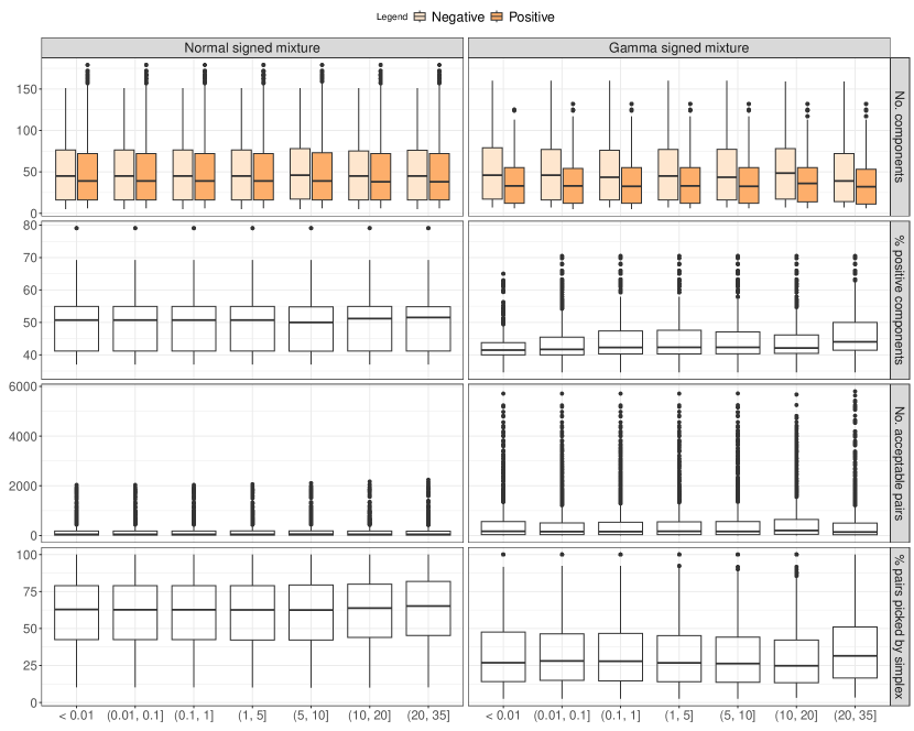
Figure 2: Summaries per vanilla average acceptance rate categories (x-axis in %) of the 2,800 randomly generated signed mixtures of, respectively, Normal distributions (left) and Gamma distributions (right): number of positive and negative weight components (top row), proportion of positive weight components in the model (second row), number of acceptable pairs in the model (third row) and proportion of acceptable pairs selected by the simplex algorithm (bottom row).

Comments

The running time of our method does not depend significantly of the user-specified acceptance rate nor the tolerance level (see Figure 3). However we can point out a consistent pattern regarding the influence of both $\delta$ and $\varepsilon$. Allowing a larger tolerance level leads to a reduced cost since it implies building a partition with less elements. However opting for a larger acceptance rate happens to increase the running time. In such settings, we end up with a larger domain to partition and a tolerance level restricted to a smaller range. Hence this results in increasing the number of partition terms, as we aim at a more precise piecewise approximation of the signed mixture. Our method is not designed to efficiently achieve acceptance rate arbitrary close to 1. Instead, users can benefit from reasonably lowering the acceptance rate $\delta$. Obviously, this holds as long as $\delta$ remains larger than the vanilla acceptance probability and the simulation cost does not exceed the advantage of the stratification.

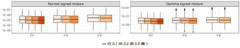
Figure 3: Running time (in sec.) of the stratified method with respect to user-specified acceptance rate $\delta$ (x-axis) and tolerance level $\epsilon$ (eps) for the 2,800 randomly generated signed mixtures of, respectively, Normal distributions (left) and Gamma distributions (right).

The relative efficiency of our stratified solution compared to the vanilla ranges from around $10^{-5}$ to $10^{5}$ and unsurprisingly decreases with the vanilla average acceptance probability (see Figure 4, top row). The stratified approach far outperforms the vanilla method on challenging situations, that is when an accept-reject from the positive part would lead to an average acceptance rate lower than 1%, a domination found even for very small samples. For a hundred samples, sampling from the positive part of the signed mixture becomes equivalent to, if not better than, the stratified solution when the vanilla average acceptance probability exceed 5%. For larger sample sizes, the relative efficiency remains in general larger than $1$. Furthermore, we point out that the median running time of our method for a given sample size is quite stable across the different categories of vanilla acceptance rates and mostly lower than the second (see Figure 4, second row). In comparison, the median running time of the vanilla method strongly depends on its associated acceptance probability (see Figure 4, third row). This asymmetry means that in situations where the vanilla method performs better, the actual computational benefit is of a negligible scale. Conversely, our method presents a reduction of the simulation cost that is more than substantial in challenging settings, cutting the cost for instance from a few minutes to less than a second.

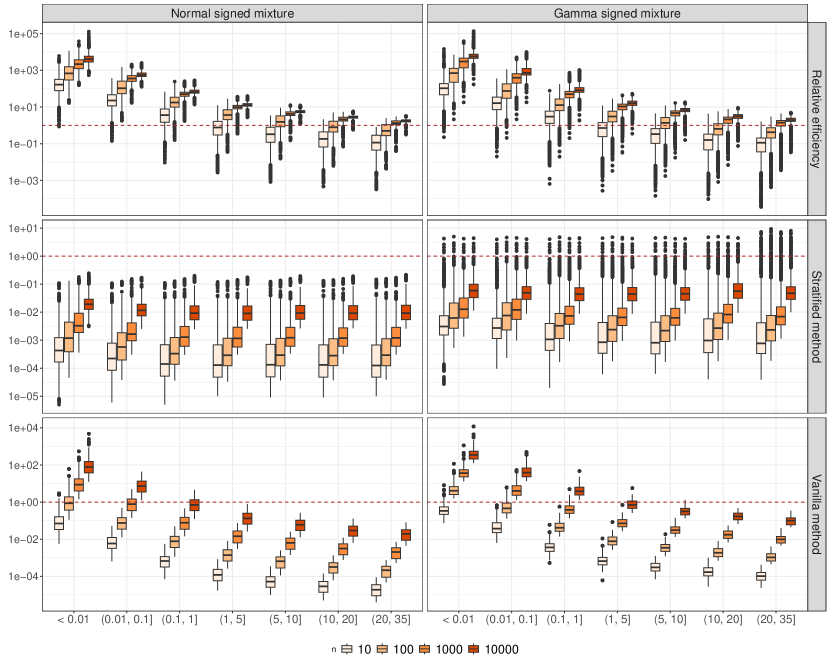
Figure 4: Time performances of accept-reject based methods per vanilla average acceptance rate categories (x-axis in %) and number of draws $n$ for the 2,800 randomly generated signed mixtures of, respectively, Normal distributions (left) and Gamma distributions (right): relative efficiency of the vanilla method compared to the stratified method (top row), running time (in sec.) of, respectively, the stratified method (second row) and the vanilla method (bottom row).

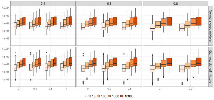
Figure 8: Relative efficiency of the vanilla method compared to the stratified method with respect to user-specified acceptance rate $\delta$, tolerance level $\epsilon$ (x-axis) and number of draws $n$, for the 2,800 randomly generated signed mixtures of, respectively, Normal distributions (top row) and Gamma distributions (bottom row).

In the stratified scheme, we have a better control of the simulation cost, even in the presence of negative weight residuals (see Figure 7), due to the acceptance rate constraint on each pairs. This explains the general median stability we observe on Figure 4 regardless the overall weight of the positive part in the model. The major elements of influence are the computation of the partition and of the pairing using the simplex method. Regarding the partition, we already observed that it does not alter strongly the computational cost of our solution and hence the relative efficiency compared to the vanilla method, but it can be further confirmed with Figure 8 in Appendix. As for the pairing step, Figure 5 illustrates that the number $|E|$ of acceptable pairs has a negative effect in terms of computational budget. Indeed, the simplex algorithm is then used to solve an optimization problem involving $2|E|$ variables and $|E|+N+P$ constraints. For a moderate number of samples, the efficiency of our solution is reduced when the model contains over a thousand acceptable pairs. In this regime the simplex may prove more time consuming than simulating even numerous random variables.

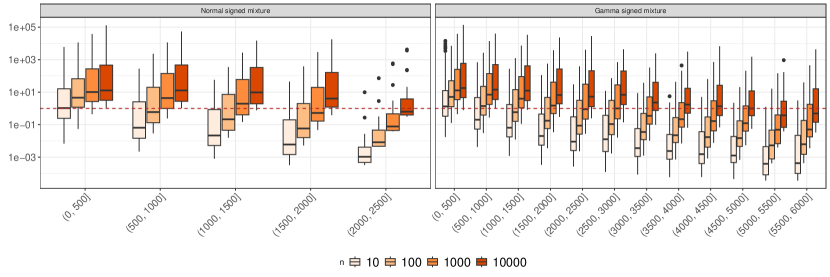
Figure 5: Relative efficiency of the vanilla method compared to the stratified method with respect to the number of acceptable pairs (x-axis) and the number of draws $n$, for the 2,800 randomly generated signed mixtures of, respectively, Normal distributions (left) and Gamma distributions (right).

The computation of a numerical inverse of the cdf does not exhibit practical interest over our accept-reject based method from a computational perspective (see Figure 6). Indeed, the median relative efficiency is close to 1, if not greater while we only generate samples from an approximated probability measure. This surrogate quantile function solely alleviates the cost of the vanilla method in low acceptance situations, a specific setting for which we provide an efficient and exact solution.

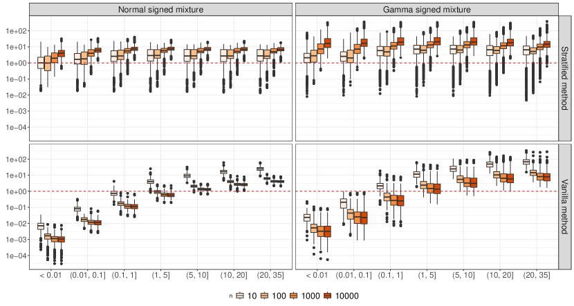
Figure 6: Relative efficiency of the numerical inverse cdf compared, respectively, to the stratified method (top row) and the vanilla method (bottom row) per vanilla average acceptance rate categories (x-axis in %) and number of draws $n$ for the 2,800 randomly generated signed mixtures of, respectively, Normal distributions (left) and Gamma distributions (right).

5 Conclusions

The challenge of simulating a signed mixture (1) surprisingly differs from the standard simulation of an unsigned mixture in that the negative components of (1) have no natural association with a latent variable. It thus proves impossible to directly eliminate simulations that issue from these negative terms, i.e., to formalize a negative version of accept-reject and one has to resort to more rudimentary approaches. As discussed above, sampling from a signed mixture using only the positive part of the density may prove cumbersome, especially when the weight of the latter is small. While elementary, our alternative approach achieves noticeably superior computational performances by combining a simplex step towards identifying an efficient decomposition of the model into a well-balanced set of two-component mixtures, and a piecewise constant approximation of these two-component distributions. Controlling a lower bound on the average acceptance rate ensures steady performance, regardless of the overall weight of the positive part. Furthermore, this alternative performs most satisfactorily relative to the inverse cdf approach, a feat explained in part by the necessity to numerically invert the cdf, even in cases when the quantile function of both positive and negative components is known.

Appendix A Two-component signed mixtures

A.1 Lower bound property

Lemma 3.

Assuming two separate probability density functions $f$ and $g$ such that $g$ is absolutely continuous with respect to $f$, then

$$a^{\star}=\sup_{\operatorname*{supp}(f)}\frac{g}{f}>1.$$ (14)

Proof.

Let assume $a^{\star}\leq 1$ and denote $E=\{x\in\operatorname*{supp}(f)\;|\;f(x)=g(x)\}$. We have for all $x\in\operatorname*{supp}(f)\setminus E$, $g(x)<f(x)$ and

$$\int_{E}g(x)\mathrm{d}x=\int_{E}f(x)\mathrm{d}x\quad\text{and}\quad\int_{\operatorname*{supp}(f)\setminus E}g(x)\mathrm{d}x<\int_{\operatorname*{supp}(f)\setminus E}f(x)\mathrm{d}x.$$ (15)

Since $\operatorname*{supp}(g)\subseteq\operatorname*{supp}(f)$, we thus have

$$1=\int_{\operatorname*{supp}(f)}g(x)\mathrm{d}x<\int_{E}f(x)\mathrm{d}x+\int_{\operatorname*{supp}(f)\setminus E}f(x)\mathrm{d}x=1.$$ (16)

Reductio ad absurdum complete. ∎

A.2 Results on stratified sampling scheme

A.2.1 Average acceptance probability of Algorithm 1

Behaviour in the tails

The distribution $m$ restricted to $D_{0}$ satisfies

$$\frac{1}{m(D_{0})}m(x)\mathds{1}_{D_{0}}(x)\leq\frac{af(D_{0})}{(a-1)m(D_{0})}\frac{1}{f(D_{0})}f(x)\mathds{1}_{D_{0}}(x).$$

To get one sample from $m$ restricted to $D_{0}$, we need on average

$$M_{0}=\frac{af(D_{0})}{(a-1)m(D_{0})}$$

samples from the distribution $f$ truncated to $D_{0}$.

Behaviour in $D_{1},\ldots D_{n}$

The distribution $m$ restricted to $D_{i}$ satisfies

$$\frac{1}{m(D_{i})}m(x)\mathds{1}_{D_{i}}(x)\leq\frac{h_{i}|D_{i}|}{(a-1)m(D_{i})}\frac{1}{|D_{i}|}\mathds{1}_{D_{i}}(x).$$

To get one sample from $m$ restricted to $D_{i}$, we need on average

$$M_{i}=\frac{h_{i}|D_{i}|}{(a-1)m(D_{i})}$$

samples from the uniform distribution on $D_{i}$.

Global behaviour

To get one sample from $m$, we need to propose on average

$$\sum_{i=0}^{n}m(D_{i})M_{i}=\frac{a}{a-1}f(D_{0})+\frac{1}{a-1}\sum_{i=1}^{n}h_{i}|D_{i}|=M$$

random variables.

Remark 1.

Sampling from distribution $f$ restricted to $D_{0}$ is not necessarily straightforward and might require an accept reject scheme as well. Both methods based on piecewise proposals have nevertheless still the same acceptance probability on average. If we need $N_{0}$ samples from a proposal to get one sample from $f$ restricted to $D_{0}$, Algorithm 1 then requires simulating

$$\tilde{M}=\frac{a}{a-1}f(D_{0})N_{0}+\frac{1}{a-1}\sum_{i=1}^{n}h_{i}|D_{i}|$$

random variables. Conversely, sampling from the dominating piecewise function would require

$$M\left\{\frac{af(D_{0})}{M(a-1)}N_{0}+\frac{1}{M(a-1)}\sum_{i=1}^{n}h_{i}|D_{i}|\right\}=\tilde{M}$$

random variables.

A.2.2 Lemma 1

Proof.

We have

$$\frac{1}{a-1}\sum_{i=1}^{n}h_{i}|D_{i}|\overset{}{\underset{n\rightarrow+\infty}{\longrightarrow}}\int_{\operatorname*{supp}(f)\setminus D_{0}}m(x)\mathrm{d}x=1-\frac{af(D_{0})-g(D_{0})}{a-1}.$$

Hence, for all $\varepsilon>0$, there exists $n_{\varepsilon}$, such that for all $n\geq n_{\varepsilon}$

$$\left|M-\frac{a-1+g(D_{0})}{a-1}\right|\leq\varepsilon.$$

Given $\varepsilon\in[0,(1-\delta)/\delta)$, if

$$\min\left[1,\frac{(a-1)\{1-\delta(\varepsilon+1)\}}{\delta}\right]=1,$$

then

$$\frac{a}{a-1}+\varepsilon\leq\frac{1}{\delta}\quad\text{and}\quad\forall n\geq n_{\varepsilon},\quad M\leq\frac{a}{a-1}+\varepsilon.$$

Otherwise, we have

$$g(D_{0})=\frac{(a-1)\{1-\delta(\varepsilon+1)\}}{\delta}\quad\text{and}\quad\left|M-\frac{1}{\delta}+\varepsilon\right|\leq\varepsilon.$$

Both cases lead to $1/M\geq\delta$. ∎

Remark 2.

A direct consequence of Lemma 1 is that if we pick the partition of $\operatorname*{supp}(f)\setminus D_{0}$ such that

$$1-m(D_{0})+\varepsilon=\frac{1}{a-1}\sum_{i=1}^{n}h_{i}|D_{i}|$$

then using the assumption on $g(D_{0})$ we get

$$M=\frac{a}{a-1}f(D_{0})+1-m(D_{0})+\varepsilon=1+\frac{1}{a-1}g(D_{0})+\varepsilon=\frac{1}{\delta}.$$

A.3 Exponential families examples

Assume that, within the context of Section 2, the terms $f$ and $g$ are both distributions from the same exponential family

$$\mathcal{F}=\left\{c(\theta)h(x)\exp\{\eta(\theta)^{\top}T(x)\}\,;\,x\in\mathbb{R}^{d},\,\theta\in\Theta\subseteq\mathbb{R}^{q}\right\}.$$

A pairing of $f$ and $g$, parametrized respectively by $\theta^{+}$ and $\theta^{-}$, into a two-components signed mixture is thus possible if

$$a^{\star}=\sup_{x\in\operatorname*{supp}(f)}\{\eta(\theta^{-})-\eta(\theta^{+})\}^{\top}T(x)<+\infty.$$ (17)

A.3.1 Example of Normal distributions

Let $f\equiv\mathcal{N}(\mu^{+},\sigma_{+}^{2})$ and $g\equiv\mathcal{N}(\mu^{-},\sigma_{-}^{2})$. Since

$$-\frac{(x-\mu^{-})^{2}}{2\sigma_{-}^{2}}+\frac{(x-\mu^{+})^{2}}{2\sigma_{+}^{2}}\underset{\pm\infty}{\sim}-x^{2}\left(\frac{\sigma_{+}^{2}-\sigma_{-}^{2}}{2\sigma_{-}^{2}\sigma_{+}^{2}}\right)$$

condition (17) is fulfilled if $\sigma_{-}^{2}<\sigma_{+}^{2}$ (or if $\mu^{+}=\mu^{-}$ and $\sigma_{-}^{2}=\sigma_{+}^{2}$ which is of no interest). Assuming $\sigma_{-}^{2}<\sigma_{+}^{2}$, critical points are then solution of

$$\frac{\mu^{-}}{\sigma_{-}^{2}}-\frac{\mu^{+}}{\sigma_{+}^{2}}+2x\left(-\frac{1}{2\sigma_{-}^{2}}+\frac{1}{2\sigma_{+}^{2}}\right)=0.$$

We derive a global maximum at

$$x^{\star}=\frac{\mu^{-}\sigma_{+}^{2}-\mu^{+}\sigma_{-}^{2}}{\sigma_{+}^{2}-\sigma_{-}^{2}}.$$

Then

$$a^{\star}=\frac{\sigma_{+}}{\sigma_{-}}\exp\left\{\frac{(\mu^{+}-\mu^{-})^{2}}{2(\sigma_{+}^{2}-\sigma_{-}^{2})}\right\}.$$

Monotonicity of a two-component Normal signed mixture

Assume $f\equiv\mathcal{N}(0,1)$ and $g\equiv\mathcal{N}(\mu,\sigma^{2})$, with $\mu\geq 0$ and $\sigma<1$. The signed mixture $m$ has at most 3 extreme values. More specifically, it admits

1. a unique global maximum in $(-\infty,0]$, if

   $$a\geq\sup_{x>\mu}\frac{(x-\mu)g(x)}{\sigma^{2}xf(x)}\,;$$

2. a local maximum in $(-\infty,0]$, a local minimum and a local maximum in $[\mu,+\infty)$, otherwise.

We have for all $x\in\mathbb{R}$

$$m^{\prime}(x)=\frac{f(x)}{a-1}\left\{\psi(x)-ax\right\},\quad\text{where}\quad\psi:x\mapsto\frac{(x-\mu)g(x)}{\sigma^{2}f(x)}.$$

The number of solutions to $m^{\prime}(x)=0$ then depends on the number of intersection points between $\psi$ and $x\mapsto ax$. The assumption on two-component signed mixtures imposes $g(x)/f(x)\overset{}{\underset{x\rightarrow\pm\infty}{\longrightarrow}}0$. Since it happens at exponential speed, we also have $\psi(x)\overset{}{\underset{x\rightarrow\pm\infty}{\longrightarrow}}0$. On the other hand, for all $x\in\mathbb{R}$,

$$\psi^{\prime}(x)=\left\{(\sigma^{2}-1)x^{2}+x(2\mu-\mu\sigma^{2})+\sigma^{2}-\mu^{2}\right\}\frac{g(x)}{\sigma^{4}f(x)}.$$

A straightforward computation shows that the equation $\psi^{\prime}(x)=0$ has two distinct solutions and thus $\psi$ has a global minimum and a global maximum, respectively at

$$x_{1}=\frac{\mu}{2}+\frac{\mu-\sigma\sqrt{\mu^{2}\sigma^{2}+4-4\sigma^{2}}}{2(1-\sigma^{2})}\quad\text{and}\quad x_{2}=\frac{\mu}{2}+\frac{\mu+\sigma\sqrt{\mu^{2}\sigma^{2}+4-4\sigma^{2}}}{2(1-\sigma^{2})}.$$

Moreover, since

$$\psi^{\prime\prime}(x)=\frac{g(x)}{\sigma^{6}f(x)}\left\{(\sigma^{2}-1)^{2}x^{3}+Q_{2}(x)\right\}$$

where $Q_{2}(x)$ is a univariate polynomial of degree 2, $\psi$ changes convexity solely one time in $[x_{1},x_{2}]$. Note that $\psi^{\prime\prime}(\mu)=2\mu g(\mu)/\{\sigma^{2}f(\mu)\}\geq 0$ and thus the change of convexity happens between $\mu$ and $x_{2}$. Functions $\psi$ and $x\mapsto ax$ have then at most 3 intersection points.

If $\boldsymbol{\mu}\mathbf{=0}$,   we have a first obvious solution: $x=0$. Since $\psi$ is an odd function when $\mu=0$, the latter solution is unique if

$$a\geq\psi^{\prime}(0)=\frac{1}{\sigma^{3}}=\sup_{x>0}\frac{g(x)}{\sigma^{2}f(x)}.$$

It is the unique global maximum for $m$, which thus have the same monotonicity than $f$. Otherwise, it is a local minimum and we have two local maxima corresponding to the intersection points solution of

$$\exp\left\{\frac{x^{2}}{2\sigma^{2}}(\sigma^{2}-1)\right\}=a\sigma^{3},$$

that is $\pm 2\sigma^{2}\log(a\sigma^{3})/(1-\sigma^{2})$.

If $\boldsymbol{\mu}\mathbf{>0}$,   we do not have a closed form for the critical points. However $\psi$ is a non-positive function on $(-\infty,\mu]$, that is decreasing on $(-\infty,x_{1})$ and an increasing convex function on $(x_{1},\mu]$. Consequently, there exists a unique intersection point $y^{\star}_{1}$ on $(-\infty,0]$ that corresponds to a local maximum of $m$. The function $x\mapsto ax$ being positive on $(0,\mu]$, if there are two other intersection points, they are necessarily in $(\mu,+\infty)$. If

$$a\geq\sup_{x>\mu}\frac{(x-\mu)g(x)}{\sigma^{2}xf(x)},$$

then for all $x>\mu$, $m^{\prime}(x)<0$ and as a result $y^{\star}_{1}$ is the unique global maximum of $m$. Otherwise, we have two intersection points. The point $y^{\star}_{2}$ corresponding to a local minimum of $m$ is bound to be on $(\mu,x_{1})$. Nevertheless, note that on $(\mu,x_{1})$

$$\psi(x)-ax\leq(x-\mu)\frac{a^{\star}}{\sigma^{2}}-ax=\frac{(a^{\star}-a\sigma^{2})x-a^{\star}\mu}{\sigma^{2}}.$$

If $a^{\star}-a\sigma^{2}>0$, $m$ is decreasing between $\mu$ and $a^{\star}\mu/(a^{\star}-a\sigma^{2})$ and $y^{\star}_{2}\geq a^{\star}\mu/(a^{\star}-a\sigma^{2})$.

Remark 3.

The results for $\mu<0$ are obtained by symmetry of the problem. Finally the result for the general case of a signed mixture $m$ of $\mathcal{N}(\mu^{+},\sigma_{+}^{2})$ and $\mathcal{N}(\mu^{-},\sigma_{-}^{2})$ can be derived using that for all $x\in\mathbb{R}$

$$m(x)\propto af\left(\frac{x-\mu^{+}}{\sigma^{+}}\right)-g\left(\frac{x-\mu^{+}}{\sigma^{+}}\right),\quad\text{with}\quad\mu=\frac{\mu^{-}-\mu^{+}}{\sigma_{+}}\quad\text{and}\quad\sigma=\frac{\sigma_{-}}{\sigma_{+}}.$$

A.3.2 Example of Gamma distributions

Let $f\equiv\Gamma(\alpha^{+},\beta^{+})$, $g\equiv\Gamma(\alpha^{-},\beta^{-})$ (shape, rate parametrization). Condition (17) imposes $\alpha^{+}\leq\alpha^{-}$ and $\beta^{+}<\beta^{-}$, so that

$$(\alpha^{-}-\alpha^{+})\log x+(\beta^{+}-\beta^{-})x \overset{}{\underset{x\rightarrow 0^{+}}{\longrightarrow}}-\infty\quad\text{or}\quad 0,$$

$$(\alpha^{-}-\alpha^{+})\log x+(\beta^{+}-\beta^{-})x \overset{}{\underset{x\rightarrow+\infty}{\longrightarrow}}-\infty.$$

Assuming this, critical points are solution of

$$\frac{\alpha^{-}-\alpha^{+}}{x}+\beta^{+}-\beta^{-}=0,$$

which leads to a unique global maximum at

$$x^{\star}=\frac{\alpha^{+}-\alpha^{-}}{\beta^{+}-\beta^{-}}.$$

Then

$$a^{\star}=\begin{cases}\displaystyle\frac{\Gamma(\alpha^{+})(\beta^{-})^{\alpha^{-}}}{\Gamma(\alpha^{-})(\beta^{+})^{\alpha^{+}}}\exp\left\{(\alpha^{+}-\alpha^{-})(1-\log x^{\star})\right\}&\quad\text{if $\alpha^{+}<\alpha^{-}$,}\\ \vspace{.25\baselineskip}\\ \displaystyle\left(\frac{\beta^{-}}{\beta^{+}}\right)^{\alpha^{+}}&\quad\text{if $\alpha^{+}=\alpha^{-}$.}\end{cases}$$

Monotonicity of a two-component Gamma signed mixture

The arguments for studying the monotonicity are similar to those used for the Gaussian case. For all $x>0$,

$$m^{\prime}(x)=\frac{f(x)}{(a-1)x}\left\{\psi(x)-a(\beta^{+}x+1-\alpha^{+})\right\},\quad\text{where}\quad\psi:x\mapsto\frac{(\beta^{-}x-\alpha^{-}+1)g(x)}{f(x)}.$$

If $\boldsymbol{\alpha^{+}=\alpha^{-}}$,   first and second derivatives of $\psi$ write as

$$\psi^{\prime}(x) =\left\{\beta^{-}(\beta^{+}-\beta^{-})x+\beta^{+}+\alpha^{-}(\beta^{-}-\beta^{+})\right\}\frac{g(x)}{f(x)}$$

$$\psi^{\prime\prime}(x) =\left[\beta^{-}(\beta^{-}-\beta^{+})x-\{\beta^{+}+\beta^{-}+\alpha^{-}(\beta^{-}-\beta^{+})\}\right]\frac{(\beta^{-}-\beta^{+})g(x)}{f(x)}.$$

We thus have a unique global maximum and a single change of convexity.

• If $\alpha^{-}=\alpha^{+}>1$, then $a(1-\alpha^{+})<\psi(0)$ and $m$ admits a unique global maximum on $(0,+\infty)$.

• If $\alpha^{-}=\alpha^{+}\leq 1$, $a(1-\alpha^{+})\geq\psi(0)$ and $m$ admits a local minimum and local maximum on $(0,+\infty)$ solely when

  $$a<\sup_{x\geq 0}\frac{\beta^{-}x+1-\alpha^{-}}{\beta^{+}x+1-\alpha^{-}}\exp\left\{(\beta^{+}-\beta^{-})x\right\}.$$

  Otherwise, $m$ is decreasing on $(0,+\infty)$.

If $\boldsymbol{\alpha^{+}<\alpha^{-}}$,

$$\psi^{\prime}(x)=\Big{[}\beta^{-}(\beta^{+}-\beta^{-})x^{2} +\{\beta^{+}(1-\alpha^{-})+\beta^{-}(2\alpha^{-}-\alpha^{+})\}x$$

$$+(\alpha^{-}-\alpha^{+})(1-\alpha^{-})\Big{]}\frac{g(x)}{xf(x)}$$

The univariate polynomial has necessarily two real roots $x_{1}$ and $x_{2}$ (otherwise $\psi$ would be a continuous decreasing function on $[0,+\infty)$ and hence constant since its limit at 0 and $+\infty$ is 0). It is straightforward to show that the smallest roots is non-positive when $\alpha^{-}\leq 1$ and non-negative when $\alpha^{-}>1$ while the largest is always positive. The convex properties are identical to the Gaussian example as

$$\psi^{\prime\prime}(x)=\frac{g(x)}{x^{2}f(x)}\left\{\beta^{-}(\beta^{-}-\beta^{+})^{2}x^{3}+Q_{2}(x)\right\},$$

where $Q_{2}(x)$ is a univariate polynomial of degree 2.

• If $\alpha^{+}<1$, then $a(1-\alpha^{+})>0$. $m$ admits a local minimum and local maximum on $(\max\{0,(\alpha^{-}-1)/\beta^{-}\},+\infty)$ solely when

  $$a<\sup_{x\geq 0}\frac{\{\beta^{-}x+1-\alpha^{-}\}g(x)}{\{\beta^{+}x+1-\alpha^{+}\}f(x)}.$$

  Otherwise, $m$ is decreasing on $(0,+\infty)$.

• If $\alpha^{+}\geq 1$, then $a(1-\alpha^{+})\leq 0$. The behaviour depends on the relative position of the modes of each component.

  • If $\beta^{-}(\alpha^{+}-1)<\beta^{+}(\alpha^{-}-1)$, then $m$ admits a local maximum in $[0,(\alpha^{+}-1)/\beta^{+}]$. It is then decreasing on $[(\alpha^{+}-1)/\beta^{+},+\infty)$ when

    $$a\geq\sup_{\beta^{+}x+1-\alpha^{+}>0}\frac{\{\beta^{-}x+1-\alpha^{-}\}g(x)}{\{\beta^{+}x+1-\alpha^{+}\}f(x)}.$$

    Otherwise, $m$ admits a local minimum and a local maximum within the latter interval.

  • If $\beta^{-}(\alpha^{+}-1)>\beta^{+}(\alpha^{-}-1)$, then $m$ admits a local maximum in $[(\alpha^{+}-1)/\beta^{+},+\infty)$. On $[0,(\alpha^{+}-1)/\beta^{+}]$, $m$ is increasing when

    $$a\geq\sup_{\beta^{-}x+1-\alpha^{-}<0}\frac{\{\beta^{-}x+1-\alpha^{-}\}g(x)}{\{\beta^{+}x+1-\alpha^{+}\}f(x)}.$$

    Otherwise, $m$ admits a local maximum and a local minimum within the latter interval.

  • If $\beta^{-}(\alpha^{+}-1)=\beta^{+}(\alpha^{-}-1)$, both component have the same mode that is the unique global maximum of $m$ when

    $$a\geq\sup_{\beta^{+}x+1-\alpha^{+}\neq 0}\frac{\{\beta^{-}x+1-\alpha^{-}\}g(x)}{\{\beta^{+}x+1-\alpha^{+}\}f(x)},$$

    and a local minimum otherwise. In the latter situation, $m$ admits two local maxima, one in $(0,(\alpha^{+}-1)/\beta^{+})$ and one in $((\alpha^{+}-1)/\beta^{+},+\infty)$.

A.3.3 Construction of the partition

We compute $D_{0}=(q_{\alpha},q_{1-\alpha})^{c}$, where $q_{\alpha}$ and $q_{1-\alpha}$ are respectively $\alpha$ and $1-\alpha$-quantiles of $g$, with

$$\alpha=\frac{(a-1)\{1-\delta(\varepsilon+1)\}}{2\delta}.$$

In the specific setting of a two-component Gamma signed mixture with both shape parameters larger than 1, we consider $D_{0}=[q_{1-2\alpha},+\infty)$.

We partition $D_{0}^{c}$ into $S$ subsets $D_{1},\ldots,D_{S}$ relying on the monotonic properties of the signed mixture. The aim is to decide whether, on subdivisions $[x_{i},x_{i+1}[$ of $D_{i}$, we use

$$(\mathrm{A})\quad h_{i}=\sup_{[x_{i},x_{i+1}[}(af-g)(x)\quad\text{or}\quad(\mathrm{B})\quad h_{i}=\sup_{[x_{i},x_{i+1}[}af(x)-\inf_{[x_{i},x_{i+1}[}g(x).$$

On each subset, the signed mixture has one of the following properties:

1. the signed mixture is a monotonic function. On such subset, we use the version (A) on every subdivision $[x_{i},x_{i+1}[$;

2. the signed mixture changes monotonicity only once on the subset. For all subdivisions $[x_{i},x_{i+1}[$ such that $m^{\prime}(x_{i})m^{\prime}(x_{i+1})>0$, we use the version (A). Otherwise, we use the version (B) but that happens solely once;

3. the signed mixture changes monotonicity more than once on the interval. On such subset, we use the version (B) on every subdivision $[x_{i},x_{i+1}[$.

Note that for two-component Gamma and Normal signed mixtures, we can restrict ourselves to usie only the first two types of subsets by numerically computing some of the local extrema.

For a given subset $D_{s}$, $1\leq s\leq S$, we start with the partition $[x_{1},x_{2}[,\ldots,[x_{n-1},x_{n}[$, such that $x_{i+1}-x_{i}=|D_{0}|/100$, $1\leq i\leq n$. The length of each partition element of $D_{s}$ is divided by two until we achieve

$$\sum_{x_{i}\in D_{s}}(x_{i+1}-x_{i})h_{i}=m(D_{i})+\frac{\varepsilon}{S+1}.$$

Appendix B Numerical inversion of the cdf

Consider $n$ ordered points $q_{1},\ldots,q_{n}$ in the support of $f$ and $p_{1},\ldots,p_{n}$ the value of the cdf associated with $m$ at these points, that is $p_{i}=m((-\infty,q_{i}])$, $1\leq i\leq n$. Furthermore, set a user-specified precision $\varepsilon$. In the paper, we used $\varepsilon=10^{-10}$.

Step A

Assume we have $u\in[p_{i},p_{i+1}]$. We compute the preimage $q^{\star}$ of $u$ by the affine transformation

$$x\mapsto\frac{p_{i+1}-p_{i}}{q_{i+1}-q_{i}}x+\frac{p_{i}q_{i+1}-p_{i+1}q_{i}}{q_{i+1}-q_{i}}.$$

Then we compute the cdf at $q^{\star}$ and denote $p^{\star}$ its value. This yields a new interval containing $u$ that is strictly included in $[p_{i},p_{i+1}]$. We now apply the same procedure on that interval. We repeat the process until we get a value $p^{\star}$ such that $|u-p^{\star}|<\varepsilon$.

Step B

If we deal with a distribution that has an unbounded support, tails should be treated separately. Assume we have $u<p_{1}$. We use a scheme similar to the above except we take the preimage by the affine transformation based on the two first points $(p_{1},p_{2})$ larger than $u$. Here we stop when we find a point $p^{\star}\leq u+\varepsilon$. If $u>p_{n}$, the reasoning is the same except we use the last two points smaller than $u$ and we stop when $p^{\star}\geq u-\varepsilon$. Now, either this ending point satisfies $|u-p^{\star}|<\varepsilon$, or we apply Step A starting with the interval $[p^{\star},p_{1}]$ for left tail or $[p_{n},p^{\star}]$ for right tail.

Appendix C Random generator of signed mixture models

We used two different methods to generate the benchmark models. Both methods start by randomly setting an initial number $K$ of positive weight components in the model. The number $K$ is drawn uniformly between $k_{\min}$ and $k_{\max}$ for the following sets $\{5,\ldots,10\}$, $\{10,\ldots,30\}$, $\{30,\ldots,50\}$, and $\{50,\ldots,100\}$. Once the number of positive weight components is set, we randomly draw the associated parameter values.

• For Normal signed mixtures, the mean $\mu^{+}$ is drawn uniformly in $[0,20]$ and the standard deviation is drawn according to a Gamma distribution $\Gamma(3,2.5)$ (shape, rate parametrization).

• For Gamma signed mixtures, the shape parameter $\alpha^{+}$ is drawn according to a Gamma distribution $\Gamma(4,0.5)$ and the rate parameter $\beta^{+}$ to a Gamma distribution $\Gamma)(2,0.7)$.

We then randomly set the number of negative weight components (1 or 2) that are initially related to each positive weight component. Parameter value for the negative components as well as the weights are then computed to ensure a benchmark model for which the vanilla average acceptance rate $p$ ranges in $[p_{\min},p_{\max}]$ for the following sets $[0,10^{-4}]$, $(10^{-4},0.001]$, $(0.001,0.01]$, $(0.01,0.05]$, $(0.05,0.1]$, $(0.1,0.2]$ and $(0.2,0.3]$. For each set of values for $K$ and $p$ and for each method, we generated 50 benchmarks.

C.1 First method

The first method is based on properties of two-component signed mixtures. For a given positive weight component, we compute the parameter value of the associated negative weight component such that $a^{\star}\in[1/(1-p_{\max}),1/(1-p_{\min})]$. The weights for this two-signed component are the ones associated with $a^{\star}$. If the positive weight component is associated with more than one negative component, we repeat this procedure for each negative component. As a result, we thus obtain a collection of two-component signed mixtures that all have the targeted acceptance rate. A convex combination with uniform rates of these mixtures yields a signed mixture with the vanilla average acceptance probability we aim at.

If the overall acceptance rate is lower than $p_{\max}$, we randomly decide to add positive weight components that can either balance some of the negative components already included or that can balance none. We can easily determine the maximal weight to assign to such single components so the acceptance rate remains lower than $p_{\max}$. Indeed, assume we add $\tilde{K}$ positive weight components. The new normalized signed mixture writes as

$$\frac{\sum_{i=1}^{K}\omega_{i}^{+}f_{i}-\sum_{j=1}^{N}\omega_{j}^{-}g_{j}+\sum_{k=1}^{\tilde{K}}r_{k}f_{K+k}}{1+\sum_{k=1}^{\tilde{K}}r_{k}}.$$

The latter is associated with a vanilla acceptance rate lower than $p_{\max}$ as long as

$$\sum_{k=1}^{\tilde{K}}r_{k}\leq\frac{p_{\max}\sum_{i=1}^{K}\omega_{i}^{+}-1}{1-p_{\max}}.$$

In a given benchmark, a negative weight component is hence not naturally paired with a single positive weight component. This method aims at providing benchmarks such that the number of acceptable pairs in the model is quite important. They constitute a good basis to challenge the performances of the simplex method as it has to narrow down the pairs involved in a pairing from a large number of initial acceptable pairs.

C.2 Second method

After generating all the positive weight components, accounting for multiplicity when more than one negative weight component is associated, for a given positive weight component, we randomly draw parameter value of the associated negative weight component such that $a^{\star}\leq 10$. This constraint ensures the two-component signed mixture does not have a vanilla acceptance rate larger than 0.90 in the worst case scenario, making the next step easier. As opposed to the previous method, we now consider the linear combination $af-g$ with $a$ drawn uniformly in $[0,a^{\star}]$. The resulting function takes negative values on the support of $f$ and, hence, does not define a distribution anymore.

We use all the positive components $f_{i}$, $1\leq i\leq K-1$ generated, except $f$, to balance the negative part of that function. First, we make sure that all positive components together have enough mass over the set of negative values, that is the function is not negative in the tails of all the possible positive components. When necessary we add one or more positive weight components (we still denote $K$ the overall number of positive weight components). We then compute the weights $\tilde{\omega}_{i}^{+}$ such that

$$af-g+\sum_{i=1}^{K-1}\tilde{\omega}_{i}^{+}f_{i}\geq 0.$$

That yields a collection of $K$ signed mixtures, each one having solely one negative component and associated with a vanilla acceptance rate $p_{i}$. We consider a convex combination of these signed mixture to control the acceptance rate associated with the vanilla method and set it to $\min_{i}p_{i}$. This is usually not enough to ensure that $p$ ranges in $[p_{\min},p_{\max}]$. However we can easily modify the model to satisfy this constraint by adding a two-signed component mixture to the model. We select at random a positive weight component included in the model and we build from it a two-signed mixture $a^{\star}f-g$ that fulfills the constraint on $p$. The new normalized signed mixture writes as

$$\frac{\sum_{i=1}^{K}\omega_{i}^{+}f_{i}-\sum_{j=1}^{N}\omega_{j}^{-}g_{j}+\lambda(a^{\star}f-g)}{1+\lambda(a^{\star}-1)}.$$

The latter is associated with a vanilla acceptance rate lower than $p_{\max}$ as long as

$$\lambda\leq\frac{p_{\max}\sum_{i=1}^{K}\omega_{i}^{+}-1}{a^{\star}(1-p_{\max})-1}.$$

This method aims at providing benchmarks that exhibit negative weight residuals. Such benchmarks allow to study the performances of the stratified method when the residuals mixture obtained after the pairing step degrade the acceptance rate of the procedure (see Figure 7).

Appendix D Supplementary material on methods comparison

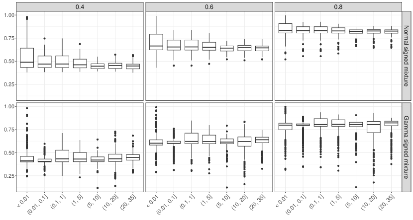
Figure 7: Theoretical acceptance rate of the stratified sampling scheme with respect to the vanilla average acceptance rate categories (x-axis in %) and user-specified acceptance rate $\delta$ for the 2,800 randomly generated signed mixtures of, respectively, Normal distributions (top row) and Gamma distributions (bottom row). An acceptance rate lower than $\delta$ signals the presence of negative weight residuals.

References

- \bibcommenthead
- Devroye [1985] Devroye, L.: Non-Uniform Random Variate Generation. Springer, New-York (1985)
- Bignami and De Matteis [1971] Bignami, A., De Matteis, A.: A Note on Sampling from Combinations of Distributions. IMA Journal of Applied Mathematics 8(1), 80–81 (1971)
- Beaulieu [1990] Beaulieu, N.C.: An infinite series for the computation of the complementary probability distribution function of a sum of independent random variables and its application to the sum of Rayleigh random variables. IEEE Transactions on Communications 38(9), 1463–1474 (1990) https://doi.org/10.1109/26.61387
- Delaigle and Hall [2010] Delaigle, A., Hall, P.: Defining probability density for a distribution of random functions. The Annals of Statistics 38(2), 1171–1193 (2010)
- Hubalek and Kuznetsov [2011] Hubalek, F., Kuznetsov, A.: A convergent series representation for the density of the supremum of a stable process. Electronic Communications in Probability 16, 84–95 (2011) https://doi.org/10.1214/ECP.v16-1601
- Zhang and Zhang [2005] Zhang, B., Zhang, C.: Finite mixture models with negative components. In: Perner, P., Imiya, A. (eds.) Machine Learning and Data Mining in Pattern Recognition, pp. 31–41. Springer, ??? (2005)
- Müller et al. [2012] Müller, P., Ali-Löytty, S., Dashti, M., Nurminen, H., Piché, R.: Gaussian mixture filter allowing negative weights and its application to positioning using signal strength measurements. In: 2012 9th Workshop on Positioning, Navigation and Communication, pp. 71–76 (2012). https://doi.org/10.1109/WPNC.2012.6268741
- Schuster et al. [2020] Schuster, I., Mollenhauer, M., Klus, S., Muandet, K.: Kernel conditional density operators. In: Chiappa, S., Calandra, R. (eds.) Proceedings of the Twenty Third International Conference on Artificial Intelligence and Statistics. Proceedings of Machine Learning Research, vol. 108, pp. 993–1004. PMLR, ??? (2020)
- Elston and Glassy [1989] Elston, D.A., Glassy, C.A.: Simulating from a mixture of exponential distributions with some negatively weighted components. Journal of Statistical Computation and Simulation 33(1), 1–9 (1989)
- Gumbel [1960] Gumbel, E.J.: Bivariate exponential distributions. Journal of the American Statistical Association 55, 698–707 (1960)
- Dantzig [1963] Dantzig, B.G.: Linear Programming and Extensions. Princeton University Press, Princeton (1963)