Design of Linear Precoders for Correlated Sources in MIMO Multiple Access Channels

Abstract

This work focuses on distributed linear precoding when users transmit correlated information over a fading Multiple-Input and Multiple-Output Multiple Access Channel. Precoders are optimized in order to minimize the sum-Mean Square Error (MSE) between the source and the estimated symbols. When sources are correlated, minimizing the sum-MSE results in a non-convex optimization problem. Precoders for an arbitrary number of users and transmit and receive antennas are thus obtained via a projected steepest-descent algorithm and a low-complexity heuristic approach. For the more restrictive case of two single-antenna users, a closed-form expression for the minimum sum-MSE precoders is derived. Moreover, for the scenario with a single receive antenna and any number of users, a solution is obtained by means of a semidefinite relaxation. Finally, we also consider precoding schemes where the precoders are decomposed into complex scalars and unit norm vectors. Simulation results show a significant improvement when source correlation is exploited at precoding, especially for low SNRs and when the number of receive antennas is lower than the number of transmitting nodes.

I Introduction

The simultaneous transmission of information from spatially separated devices often occurs in many wireless communications applications like Wireless Sensor Networks and mobile cellular networks. We focus on the Multiple Access Channel (MAC), also called uplink channel, where multiple user terminals transmit their data to one centralized node. We further consider the more general Multiple-Input and Multiple-Output (MIMO) case where both the receiver and the individual users are equipped with several antennas. More specifically, we address the transmission of correlated information over the fading MAC using linear precoding.

WSNs is an example of a scenario where the assumption of sources transmitting statistically independent information does not often hold because the information is usually correlated. For example, the measurements of a parameter of interest (temperature, humidity, etc.) using sensors placed in a given area often produce correlated data. The traditional way to optimize such communication systems consists of maximizing the throughput by removing the source correlation and then protecting the relevant data with an appropriate channel coding scheme. This is known as the separation principle where source and channel coding are optimized separately [1]. This strategy has been shown to be optimal for multiple scenarios under certain circumstances (large block lengths, high delay, etc.), but this no longer holds for others like the transmission of correlated data over a MAC [2, 3].

An alternative approach consists in designing the transmission scheme to minimize the signal distortion while exploiting the source correlation. In this case, the source symbols are directly transformed into the corresponding channel symbols using appropriate encoding mappings. Some examples of this strategy in MAC communications are linear mappings [2, 4], non-linear mappings [5, 6, 7] or schemes based on vector quantizers [2, 8, 9]. Linear mappings show near-optimal performance for low Signal-to-Noise Ratio (SNR) values, whereas non-linear approaches more efficiently exploit high correlations in the high SNR region [10]. However, current strategies to optimize non-linear mappings for time-varying channels are computationally unaffordable in practical applications, and the alternative is to use parametric mappings adapted to the channel conditions with a small number of parameters. Linear schemes and parametric non-linear mappings are in general suboptimal for fading channels, but their performance can be improved using precoding techniques that exploit the channel knowledge at transmission.

In multiuser scenarios assuming uncorrelated information, the channel capacity can be approached with non-linear strategies such as Costa precoding [11] or Tomlinson-Harashima precoding [12, 13]. Linear precoding, however, often provides a reasonable performance with much lower complexity [14, 15]. Linear precoders usually aim at optimizing metrics like the Signal-to-Interference-Noise Ratio (SINR) [16], the sum- Mean Squared Error (MSE) [17, 18], or the balancing of individual distortions [19, 20]. In general, these approaches improve the performance of digital communications and, also, lowering the MSE is optimal from the point of view of analog communications where the ultimate goal is minimizing the signal distortion.

In this work, we address the optimization of distributed linear precoding techniques that exploit the source correlation to minimize the signal distortion in the fading MIMO MAC. Unlike the uncorrelated sources case, the source covariance matrix is no longer diagonal and the resulting optimization problems cannot be reformulated in a convex form. In spite of that, optimal solutions are obtained for some particular scenarios, while suboptimal approaches are considered in the more general case. The optimization of linear transceivers according to the MSE metric has already been considered for correlated sources and single-user MIMO channels [4], and for the case of bivariate Gaussian sources and collaborative Gaussian MAC [21]. The design of linear filters based on the SINR is addressed in [22]. However, they considered an array model and a particular error model to perform the analysis, and the precoding scalar factors are set to one. Also, some authors addressed the linear precoding of correlated sources through the design of Code Division Multiple Access (CDMA) signatures where the users transmit their symbols using several channel uses over a fading MAC and the receiver has a single antenna [23, 24].

The remaining of this paper is organized as follows. Section II presents the communication model considered in this work. In Section III, we address the design of linear precoding schemes for the general MIMO MAC and present three approaches which provide different alternatives to exploit source correlation. Section IV focuses on the Multiple-Input and Single-Output (MISO) MAC scenario where the linear precoders are obtained by using Semidefinite Programming (SDP) to simplify the optimization problem. Section V provides an analytical solution for the two-user Single-Input and Multiple-Output (SIMO) MAC precoder. Section VI presents the results of simulation experiments carried out to illustrate the performance of the proposed strategies. Finally, Section VII is devoted to the conclusions.

I-A Contributions

In this work, we propose different approaches to optimize the linear precoding of correlated Gaussian sources according to sum-MSE:

• A closed-form expression for the optimal linear precoder that minimizes the sum-MSE in the two-user SIMO MAC scenario.

• An SDP approach for scenarios with an arbitrary number of users and a single receive antenna. This solution leads to a convex optimization problem that can be efficiently solved by interior point methods.

• For the general case of multiple antennas at transmission and reception, two approaches are considered. The first one is a heuristic approximation assuming all users are decoded with the same receive filter. The second one is based on splitting the precoding vectors into a complex-valued scalar and a unit-norm direction vector. Direction vectors are obtained using either Maximum Ratio Transmitter (MRT) or nullspace-directed SVD (Nu-SVD) that do not take into account source correlation. However, gain factors are determined to minimize the sum-MSE by exploiting source correlation.

II System Model

Figure 1: Block-diagram of a fading MIMO MAC system with $K$ users, linear precoders, and a linear receiver.

Let us consider the fading MIMO MAC system model shown in Fig. 1 where $K$ individual users with $N_{T}$ antennas each send correlated information to a common receiver with $N_{R}$ antennas. The $k$-th user sends one source symbol per channel use $s_{k}$. The vector $\mathbf{s}=[s_{1},s_{2},\ldots,s_{K}]^{T}$ comprising all users source symbols follows a multivariate complex-valued distribution with zero mean and covariance matrix $\mathbf{C}_{\mathbf{s}}=E\left[\mathbf{s}\mathbf{s}^{H}\right]$. The superindices ^T and ^H represent the transpose and Hermitian operators, respectively. The elements $[\mathbf{C}_{\mathbf{s}}]_{i,j}=\rho_{i,j}$ represent the correlation between the $i$-th and $j$-th source symbols. Without loss of generality, we will assume that $\rho_{i,i}=1~{}\forall i$ and $0\leq\rho_{i,j}\leq 1~{}\forall i,j$ such that $i\neq j$.

The source symbols are individually precoded at each user using a linear scheme and the resulting symbols are then transmitted to the receiver over their corresponding fading channels. We will consider a small-scale fading model, disregarding the attenuation caused by free space propagation and other effects. The received MAC signal is represented as

$$\mathbf{y}=\sum_{k=1}^{K}\mathbf{H}_{k}\mathbf{p}_{k}s_{k}+\mathbf{n},$$ (1)

where $\mathbf{p}_{k}\in\mathbb{C}^{N_{T}\times 1}$ and $\mathbf{H}_{k}\in\mathbb{C}^{N_{R}\times N_{T}}$ are the $k$-th user linear precoding vector and MIMO channel response, respectively; and $\mathbf{n}=[n_{1},\ldots,n_{N_{R}}]^{T}$ represents the complex-valued Additive White Gaussian Noise (AWGN) such that $\mathbf{n}\sim\mathcal{N}_{\mathbb{C}}(\mathbf{0},\sigma_{n}^{2}\mathbf{I})$. An individual power constraint is imposed at each transmitter, which is given by $\mathbf{p}_{k}^{H}\mathbf{p}_{k}\leq T_{k},k=1,\ldots,K$ since the power of the source symbols is assumed to be equal to $1$. The received signal (1) can be rewritten in a more compact form as

$$\mathbf{y}=\mathbf{H}\mathbf{P}\mathbf{s}+\mathbf{n},$$ (2)

where $\mathbf{H}=[\mathbf{H}_{1}\cdots\mathbf{H}_{K}]$ and $\mathbf{P}=\operatorname{blockdiag}\left(\mathbf{p}_{1},\ldots,\mathbf{p}_{K}\right)$, with $\operatorname{blockdiag}(\cdot)$ the operator that constructs a block-diagonal matrix and puts the matrices received as arguments on its main diagonal, setting the off-diagonal elements to zero. Finally, a linear estimate of the source symbols $\hat{\mathbf{s}}=[\hat{s}_{1},\hat{s}_{2},\ldots,\hat{s}_{K}]^{T}=\mathbf{W}^{H}\mathbf{y}$ is computed, $\mathbf{W}$ being the linear receiver filter response.

In the ensuing sections, we consider several strategies to determine the linear precoders in $\mathbf{P}$ for the described MIMO MAC system model.

III MIMO MAC Linear Precoding

Along this work, the distortion between the source and the estimated symbols will be measured in terms of the sum-MSE criterion as

$$\xi_{\text{sum}}=\mathbb{E}\left[\sum\limits_{k=1}^{K}|s_{k}-\hat{s}_{k}|^{2}\right]=\mathbb{E}\left[\operatorname{tr}\left((\mathbf{s}-\hat{\mathbf{s}})(\mathbf{s}-\hat{\mathbf{s}})^{H}\right)\right].$$ (3)

For given precoders and channel responses, $\mathbf{P}$ and $\mathbf{H}$, the linear Minimum Mean Squared Error (MMSE) receiving filter is

$$\mathbf{W}^{H}=\mathbf{C}_{\mathbf{s}}\mathbf{P}^{H}\mathbf{H}^{H}\left(\mathbf{H}\mathbf{P}\mathbf{C}_{\mathbf{s}}\mathbf{P}^{H}\mathbf{H}^{H}+\frac{1}{\sigma_{n}^{2}}\mathbf{I}\right)^{-1}.$$ (4)

Substituting (4) into (3) leads to the following expression for the sum-MSE [25]

$$\xi_{\text{sum}}=f(\mathbf{P})=\operatorname{tr}\left(\frac{1}{\sigma_{n}^{2}}\mathbf{P}^{H}\mathbf{H}^{H}\mathbf{H}\mathbf{P}+\mathbf{C}_{s}^{-1}\right)^{-1}.$$ (5)

The optimal linear MIMO MAC precoder that minimizes the sum-MSE is hence determined from the following constrained optimization problem

$$\underset{\mathbf{p}_{1},\ldots,\mathbf{p}_{K}}{\arg\min}~{}~{} \operatorname{tr}\left(\frac{1}{\sigma_{n}^{2}}\mathbf{P}^{H}\mathbf{H}^{H}\mathbf{H}\mathbf{P}+\mathbf{C}_{s}^{-1}\right)^{-1}$$ (6)

$$s.t.~{}~{} \mathbf{p}_{k}^{H}\mathbf{p}_{k}\leq T_{k},\forall k\in[1,K],$$

$$\mathbf{P}=\operatorname{blockdiag}\left(\mathbf{p}_{1},\ldots,\mathbf{p}_{K}\right),$$

where $\mathbf{p}_{k}^{H}\mathbf{p}_{k}\leq T_{k}$ represents the individual power constraints and $\mathbf{P}=\operatorname{blockdiag}\left(\mathbf{p}_{1},\ldots,\mathbf{p}_{K}\right)$ arises from the restriction that users do not cooperate and, therefore, the source symbols are individually precoded at each transmitter.

The optimization problem in (6) is non-convex on $\mathbf{P}$ when sources are correlated. When $\mathbf{C_{s}}=\mathbf{I}$ (i.e. uncorrelated sources), (6) can be reformulated in convex form over the transmit covariance matrices $\mathbf{P}\mathbf{C_{s}}\mathbf{P}^{H}$ using the matrix inversion lemma (see [17] and references therein). A convex reformulation has also been adopted when designing CDMA signatures for the transmission of correlated sources with one receive antenna [23, 24]. By dropping the restrictions over the shape of $\mathbf{P}$, e.g., allowing users to cooperate in the MAC or considering a Broadcast Channel (BC), idempotent matrices $\mathbf{C_{s}}$ are also valid. Nevertheless, none of these strategies are valid to obtain a convex reformulation of (6), since they cannot be applied to the case of distributed non-cooperative users as is usually the case in the MAC. However, some interesting conclusions can be drawn for asymptotic cases assuming that the entries of the channel matrix are independent and identically distributed (i.i.d.) complex-valued Gaussian random variables with zero mean and unit variance, i.e., $[\mathbf{H}]_{i,j}\sim\mathcal{N}_{\mathbb{C}}(0,1)$:

• When $N_{T}=1,N_{R}\rightarrow\infty$ and the number of users is fixed, the product $\frac{1}{N_{R}}\mathbf{H}^{H}\mathbf{H}$ converges almost surely to the identity matrix [26]. In this case, the MSE can be approximated as

  $$\operatorname{tr} \left(\frac{1}{\sigma_{n}^{2}}\mathbf{P}^{H}\mathbf{H}^{H}\mathbf{H}\mathbf{P}+\mathbf{C}_{s}^{-1}\right)^{-1}$$ (7)

  $$=\frac{1}{N_{R}}\operatorname{tr}\left(\frac{1}{N_{R}\sigma_{n}^{2}}\mathbf{P}^{H}\mathbf{H}^{H}\mathbf{H}\mathbf{P}+\frac{1}{N_{R}}\mathbf{C}_{s}^{-1}\right)^{-1}$$

  $$\approx\frac{1}{N_{R}}\operatorname{tr}\left(\frac{1}{\sigma_{n}^{2}}\mathbf{P}^{H}\mathbf{P}\right)^{-1}=\frac{\sigma_{n}^{2}}{N_{R}}\sum_{k=1}^{K}\frac{1}{|p_{k}|^{2}},$$

  and therefore the optimum power allocation is $p_{k}^{o}=\sqrt{T_{k}},\forall k$.

• In the high SNR regime ($\sigma_{n}^{2}\rightarrow 0$), the weight of the source correlation matrix in (6) is negligible. Therefore, the solutions for uncorrelated scenarios apply and $p_{k}^{o}=\sqrt{T_{k}}$.

In the described scenarios, good solutions for the optimal linear precoder are expected to be obtained without considering source correlation. In the next subsections, different approaches are studied for the design of linear precoders that exploit the source correlation.

III-A Projected Gradient Algorithm

A first approach to solve (6) is by means of a projected steepest-descent or gradient algorithm, where the precoding matrix $\mathbf{P}$ is updated at each iteration by

$$\mathbf{P}^{(i+1)}=t\left(\mathbf{P}^{i}+\mu^{i}\nabla f(\mathbf{P}^{i})\right),$$ (8)

where $i$ indicates the iteration number, $\mu$ is the algorithm step size, $\nabla f(\mathbf{P})$ is the gradient vector of the cost function $\xi_{\text{sum}}=f(\mathbf{P})$ with respect to $\mathbf{P}$ given by

$$\nabla f(\mathbf{P})=\frac{\partial f(\mathbf{P})}{\partial\mathbf{P}^{*}}=-\frac{2}{\sigma_{n}^{2}}\mathbf{H}^{H}\mathbf{H}\mathbf{P}\left(\frac{1}{\sigma_{n}^{2}}\mathbf{P}^{H}\mathbf{H}^{H}\mathbf{H}\mathbf{P}+\mathbf{C}_{s}^{-1}\right)^{-2},$$

and $t\left(\cdot\right)$ projects the precoder into the space of feasible solutions given by the set of constraints. In our case, the projection normalizes the power of the user precoders in $\mathbf{P}$ that exceeds their corresponding constraints and sets the off-diagonal elements to zero. Hence, $t\left(\cdot\right)$ is a projector onto a closed convex set, thus it is non-expansive, i.e., $\|t(\mathbf{P}_{1})-t(\mathbf{P}_{2})\|_{F}\leq\|\mathbf{P}_{1}-\mathbf{P}_{2}\|_{F}$ [27, Prop. 2.1.3]. Applying this property and with $\mathbf{P}^{o}$ the optimum of the cost function, we get $\|\mathbf{P}^{(i)}-\mathbf{P}^{o}\|_{F}^{2}\geq\|\mathbf{P}^{(i+1)}-\mathbf{P}^{o}\|_{F}^{2}\geq\|t(\mathbf{P}^{(i+1)})-\mathbf{P}^{o}\|_{F}^{2}$ and convergence to a local optimum is guaranteed as long as the step size is properly adjusted at each iteration by using, e.g., a line or Armijo’s search [27]. Since the problem is non-convex, the convergence of algorithm (8) to the global optimal solution is not guaranteed, but it always achieves a stationary point.

The computational complexity of this algorithm can be significant since the number of steps to achieve a solution with an error below some given threshold is unbounded in general. In practical terms, we have checked that its performance is as good as any other method we have investigated, and hence we will use it as a reference for comparison.

III-B Aligned MRT

In this section, we present a low complexity approach based on aligning the different users to a single receive direction. This simple design is inspired by the idea that only a small part of the signals from other users is actually an interference when the source symbols are highly correlated, and hence the received symbols can be combined constructively. This approach is especially suitable for low SNRs since the impact of the source correlation on the sum-MSE minimization is more significant at the low SNR regime, while it vanishes for high SNRs.

The selection of the receive direction is of key importance since it will determine the overall system performance. Unfortunately, the selection of the best direction taking into account the channels for all the users is a combinatorial problem. Hence, we propose a heuristic where the precoders are designed assuming that the receive filter is common for all users, i.e.

$$\underset{\mathbf{g},\mathbf{p}}{\arg\max}\max_{k}|\mathbf{g}^{H}\mathbf{H}_{k}\mathbf{p}|,~{}~{}s.t.~{}~{}\|\mathbf{g}\|=1,\|\mathbf{p}\|=1,$$ (9)

where the receive direction $\mathbf{g}$ is chosen as the channel left singular vector corresponding to the maximum singular value among all users. Given the direction vector $\mathbf{g}$, the precoder for the $k$-th user is computed as the vector $\mathbf{p}_{k}$ that maximizes the product $|\mathbf{g}^{H}\mathbf{H}_{k}\mathbf{p}_{k}|$, i.e.,

$$\mathbf{p}_{k}=\frac{\sqrt{T_{k}}}{\|\mathbf{H}_{k}^{H}\mathbf{g}\|}\mathbf{H}_{k}^{H}\mathbf{g}.$$ (10)

This approach hence maximizes the power of the correlated signal in the receive direction $\mathbf{g}$, because the users encode their symbols to allocate the available power into a single spatial direction. Finally, for the precoders (10), the receive filters are computed according to (4). This strategy will be termed Aligned MRT (AMRT).

III-C MRT and Nu-SVD for Correlated Sources

In this section, we focus on Maximum Ratio Transmitter (MRT) and nullspace-directed Singular Value Decomposition (SVD) algorithm (Nu-SVD), two representative linear precoding strategies for the MIMO BC and MAC. We next explain how to integrate MRT and Nu-SVD precoding in a MIMO MAC signaling scheme that exploits source correlation. The key step is to decompose the individual precoders as $\mathbf{p}_{k}=\gamma_{k}\mathbf{u}_{k}$, where $\gamma_{k}\in\mathbb{C}$ is a complex-valued gain factor and $\mathbf{u}_{k}\in\mathbb{C}^{N_{T}\times 1}$ is a unit-norm direction vector, i.e., $\|\mathbf{u}_{k}\|^{2}=1$. When considering MRT, the directions $\mathbf{u}_{k}$ are chosen to maximize the receiver SNR, i.e. $\mathbf{u}_{k}^{\text{MRT}}=\mathbf{v}_{k,1}$, where $\mathbf{v}_{k,1}$ is the right singular vector with the largest singular value in the SVD $\mathbf{H}_{k}=\mathbf{U}_{k}\boldsymbol{\Sigma}_{k}\mathbf{V}_{k}^{H}$ [28].

An alternative strategy is the iterative nullspace-directed SVD algorithm proposed for precoding in the MIMO BC [15] [14, Section V]. It can be applied to the MIMO MAC by invoking the MSE-duality to transform the receive filters in the BC into the precoders in the MAC [17, 29]. In general, this approach iteratively searches for matrices $\mathbf{P}_{\text{NSVD}}=\operatorname{blockdiag}\left(\mathbf{u}_{1}^{\text{NSVD}},\ldots,\mathbf{u}_{K}^{\text{NSVD}}\right)$ and $\mathbf{W}_{\text{NSVD}}$ such that the inter-user interference is canceled and it hence provides solutions that satisfy the condition $\mathbf{W}_{\text{NSVD}}^{H}\mathbf{H}\mathbf{P}_{\text{NSVD}}=\mathbf{I}$. This property holds both in the BC and the MAC.

In uncorrelated sources scenarios, the solutions for the gain factors $\gamma_{k}$ are trivial and are set to the maximum available power, i.e. $\gamma_{k}=\sqrt{T_{k}}$. However, source correlation can be exploited at transmission if the gain factors $\gamma_{k}$ are optimized to minimize the sum-MSE, as shown analytically in Section V for the two-user SIMO MAC and numerically in Section VI for a larger number of users. This can be done by applying the projected steepest-descent algorithm in (8) to the equivalent channels $\tilde{\mathbf{h}}_{k}=\mathbf{H}_{k}\mathbf{u}_{k}$. This approach reduces the dimension of the search space since the original problem with $N_{T}K$ variables is transformed into a search over the $K$ gain coefficients.

IV Multiuser SISO scenario

For the particular scenario with a single receive antenna and a single transmit antenna per user, i.e., $N_{R}=1,N_{T}=1$, the channel matrix reduces to a row vector $\mathbf{h}\in\mathbb{C}^{1\times N_{T}K}$ and the sum-MSE expression (5) can be rewritten by applying the matrix inversion lemma as

$$\xi_{\text{sum}}= \operatorname{tr}\left(\frac{1}{\sigma_{n}^{2}}\mathbf{P}^{H}\mathbf{h}^{H}\mathbf{h}\mathbf{P}+\mathbf{C}_{s}^{-1}\right)^{-1}$$

$$= K-\operatorname{tr}\left(\mathbf{C}_{s}\mathbf{P}^{H}\mathbf{h}^{H}\left(\mathbf{h}\mathbf{P}\mathbf{C}_{s}\mathbf{P}^{H}\mathbf{h}^{H}+\sigma_{n}^{2}\right)^{-1}\mathbf{h}\mathbf{P}\mathbf{C}_{s}\right)$$

$$= K-\frac{\mathbf{p}^{H}\mathbf{H}\mathbf{C}_{s}^{2}\mathbf{H}^{H}\mathbf{p}}{\mathbf{p}^{H}\mathbf{H}\mathbf{C}_{s}\mathbf{H}^{H}\mathbf{p}+\sigma_{n}^{2}},$$ (11)

where $\mathbf{H}=\operatorname{diag}(\mathbf{h})$, and $\mathbf{p}\in\mathbb{C}^{N_{T}K\times 1}$ stacks the diagonal elements of $\mathbf{P}^{H}$. Hence, the optimization problem can be restated as

$$\underset{\mathbf{p}}{\arg\max}~{}~{} \frac{\mathbf{p}^{H}\mathbf{H}\mathbf{C}_{s}^{2}\mathbf{H}^{H}\mathbf{p}}{\mathbf{p}^{H}\mathbf{H}\mathbf{C}_{s}\mathbf{H}^{H}\mathbf{p}+\sigma_{n}^{2}}$$ (12)

$$s.t.~{}~{} \mathbf{p}^{H}\mathbf{e}_{k}\mathbf{e}_{k}^{T}\mathbf{p}\leq T_{k},\forall k\in[1,K],$$

where $\mathbf{e}_{k}$ denotes the indicator vector. Following a similar approach to [30], the system is homogenized with $\mathbf{p}=\mathbf{q}/t$, and rewritten as

$$\underset{\mathbf{q},t}{\arg\max}~{}~{} f(\mathbf{q},t)=\frac{\mathbf{q}^{H}\mathbf{H}\mathbf{C}_{s}^{2}\mathbf{H}^{H}\mathbf{q}}{\mathbf{q}^{H}\mathbf{H}\mathbf{C}_{s}\mathbf{H}^{H}\mathbf{q}+\sigma_{n}^{2}t^{2}}$$ (13)

$$s.t.~{}~{} \mathbf{p}^{H}\mathbf{e}_{k}\mathbf{e}_{k}^{T}\mathbf{p}\leq t^{2}T_{k},\forall k\in[1,K].$$

If we denote $g(\mathbf{z})=f(\mathbf{q},t)$ with $\mathbf{z}=[\mathbf{q}^{T},t]^{T}$, it can be seen that it is invariant to scaling, i.e. $g(k\mathbf{z})=g(\mathbf{z}),k\in\mathbb{R}^{+}$. Hence, we can fix the denominator to a constant value to transform the problem as

$$\underset{\mathbf{z}}{\arg\max}~{}~{} \mathbf{z}^{H}\mathbf{A}\mathbf{z}$$ (14)

$$s.t.~{}~{} \mathbf{z}^{H}\mathbf{B}\mathbf{z}=1,$$ (15)

$$\mathbf{z}^{H}\mathbf{D}_{k}\mathbf{z}\leq 0,\forall k\in[1,K],$$ (16)

$$t\neq 0,$$ (17)

where $\mathbf{A}=\operatorname{blockdiag}(\mathbf{H}\mathbf{C}_{s}^{2}\mathbf{H}^{H},0)$, $\mathbf{B}=\operatorname{blockdiag}(\mathbf{H}\mathbf{C}_{s}\mathbf{H}^{H},\sigma_{n}^{2})$, and $\mathbf{D}_{k}=\operatorname{blockdiag}(\mathbf{e}_{k}\mathbf{e}_{k}^{T},-T_{k})$, which is a non-convex Quadratically Constrained Quadratic Programming (QCQP) problem. This problem simplifies by dropping condition (17) because for $t=0$ the constraints in (16) are fulfilled only with $\mathbf{q}=\mathbf{0}$, but then (15) is not satisfied. Hence, the feasible set is empty for $t=0$. We now define $\mathbf{Z}=\mathbf{z}\mathbf{z}^{H}$ and rewrite the optimization problem (14)-(17) as

$$\underset{\mathbf{Z}}{\arg\max}~{}~{} \operatorname{tr}(\mathbf{A}\mathbf{Z})$$ (18)

$$s.t.~{}~{} \operatorname{tr}(\mathbf{B}\mathbf{Z})=1,$$

$$\operatorname{tr}(\mathbf{D}_{k}\mathbf{Z})\leq 0,\forall k\in[1,K],$$

$$\mathbf{Z}\succeq 0,$$

where a constraint $\operatorname{rank}(\mathbf{Z})=1$ has been dropped. The problem in (18) is a SDP that can be efficiently solved with interior point methods, and it is a convex approximation of the QPQC in (14)-(17). Their solutions are not guaranteed to coincide because it is possible, for an optimal $\mathbf{Z}^{o}$ in (18), that $\operatorname{rank}(\mathbf{Z}^{*})>1$. In that case, it is necessary to resort to techniques that obtain rank-1 approximations of $\mathbf{Z}^{o}$ to estimate the optimal solution of (14)-(17). In our problem, we can obtain optimal rank-1 approximations when the solutions to (18) have a particular structure using the following lemma.

Lemma IV.1

Given an optimal solution $\mathbf{Z}^{o}$ for a problem in the form of (18) such that

$$\mathbf{Z}^{o}=\left(\begin{array}[]{cc}\bar{\mathbf{Z}}&\mathbf{v}\\ \mathbf{v}^{H}&w\end{array}\right),$$ (21)

then, if $\operatorname{rank}(\bar{\mathbf{Z}})=1$ with $\bar{\mathbf{Z}}=\mathbf{u}\mathbf{u}^{H}$, an optimal rank-1 approximation to $\mathbf{Z}^{o}$ is

$$\mathbf{Z}^{+}=\left(\begin{array}[]{cc}\mathbf{u}\mathbf{u}^{H}&\mathbf{u}\sqrt{w}\\ \mathbf{u}^{H}\sqrt{w}&w\end{array}\right),$$ (24)

and the optimal solution to problem (14) is $\mathbf{q}^{o}=\mathbf{u}$ and $t^{o}=\sqrt{w}$.

Proof:

This is straightforward by checking the structure of $\mathbf{A}$, $\mathbf{B}$ and $\mathbf{D}_{k}$, where the vectors $\mathbf{v}$ from the optimal solution are multiplied by zeros. Hence, since $\operatorname{tr}(\mathbf{AZ}^{o})=\operatorname{tr}(\mathbf{AZ}^{+})$, and the restrictions are fulfilled, i.e., $\operatorname{tr}(\mathbf{B}\mathbf{Z}^{+})=1$ and $\operatorname{tr}(\mathbf{D}_{k}\mathbf{Z}^{+})\leq 0,\forall k\in[1,K]$, we conclude that $\mathbf{Z}^{+}$ is also optimal. Hence, it optimizes (14) with the solutions given by the lemma. ∎

In case $\operatorname{rank}(\bar{\mathbf{Z}})>1$, we choose the eigenvector with the largest associated eigenvalue as approximation. Finally, the precoder is defined as $\mathbf{p}^{o}=\mathbf{u}/\sqrt{w}$. We have experimentally checked that, if $N_{T}=1$, the solutions for $\bar{\mathbf{Z}}$ obtained through the SDP are always rank-1. Hence, they are always optimal. This approach can be naturally extended to more than one transmit antenna per user by modifying the constraints, but we found that the solutions of the relaxed version of the problem are not always rank-1. Hence, we restrict our results in Section VI to $N_{T}=1$.

V Optimal Linear Precoding for the Two-User SIMO MAC

The sum-MSE minimization problem (6) is difficult to solve analytically for the general MIMO MAC. However, in this section, we will show that it can be analytically solved for the more specific two-user SIMO MAC, i.e., for the case of two single-antenna users and an arbitrary number of receive antennas. In this scenario, the precoder matrix reduces to

$$\mathbf{P}=\left(\begin{array}[]{cc}\sqrt{P_{1}}e^{-j\pi\phi_{1}}&0\\ 0&\sqrt{P_{2}}e^{-j\pi\phi_{2}}\end{array}\right),$$ (27)

where $P_{1}$ and $P_{2}$ represent the power allocated to the single-antenna users $1$ and $2$, respectively, while $\phi_{1}$ and $\phi_{2}$ represent their phase shifts. The source covariance matrix also reduces to

$$\mathbf{C}_{\mathbf{s}}=\left(\begin{array}[]{cc}1&\rho\\ \rho&1\end{array}\right),$$ (30)

where $\rho=E[s_{1}s_{2}^{*}]$ represents the source symbols correlation between the two users. Without loss of generality, we assume $\rho$ is real-valued. Particularizing (3) for this scenario, the sum-MSE is given by [2]

$$\xi_{\text{sum}}(P_{1},P_{2},\phi_{d},\sigma_{n}^{2},\rho,\mathbf{H})= \sigma_{n}^{2}\frac{2\sigma_{n}^{2}+(1-\rho^{2})(P_{1}\|\mathbf{h}_{1}\|^{2}+P_{2}\|\mathbf{h}_{2}\|^{2})}{\sigma_{n}^{4}+\sigma_{n}^{2}\upsilon+\omega},$$ (31)

where

$$\upsilon= P_{1}\|\mathbf{h}_{1}\|^{2}+P_{2}\|\mathbf{h}_{2}\|^{2}+2\rho\sqrt{P_{1}P_{2}}\Re\{e^{-j\pi\phi_{d}}\mathbf{h}_{1}^{H}\mathbf{h}_{2}\},$$

$$\omega= P_{1}P_{2}(1-\rho^{2})\left(\|\mathbf{h}_{1}\|^{2}\|\mathbf{h}_{2}\|^{2}-|\mathbf{h}_{1}^{H}\mathbf{h}_{2}|^{2}\right)=P_{1}P_{2}(1-\rho^{2})|\mathbf{H}^{H}\mathbf{H}|,$$

and $\phi_{d}=\phi_{1}-\phi_{2}$. The terms $\mathbf{h}_{1}$ and $\mathbf{h}_{2}$ correspond to the channel responses for the first and second transmitter, respectively, such that $\mathbf{H}=[\mathbf{h}_{1}\mathbf{h}_{2}]$. For two users, the optimization problem (6) simplifies to

$$\underset{P_{1},P_{2},\phi_{d}}{\arg\min}~{}~{}~{}\xi_{\text{sum}},~{}~{}s.t.~{}~{}~{}P_{1}\leq T_{1},\,P_{2}\leq T_{2}.$$ (32)

The optimal linear precoder is obtained with the help of the following two lemmas. The first one determines the optimal phases while the second determines the optimal power allocations for the optimal phases.

Lemma V.1

The optimal phases $\phi_{1}^{\text{opt}}$ and $\phi_{2}^{\text{opt}}$ for the two-user SIMO MAC linear precoder must satisfy

$$\phi_{1}^{\text{opt}}-\phi_{2}^{\text{opt}}=\phi_{d}^{\text{opt}}=\underset{\phi_{d}}{\arg\max}~{}\Re\{e^{-j\pi\phi_{d}}\mathbf{h}_{1}^{H}\mathbf{h}_{2}\}=\arg(\mathbf{h}_{1}^{H}\mathbf{h}_{2}).$$ (33)

Proof:

The variable $\phi_{d}$ is only present in the denominator of (31), in the term $\Re\{e^{-j\pi\phi_{d}}\mathbf{h}_{1}^{H}\mathbf{h}_{2}\}$. Thus, for any transmit powers $P_{1}$ and $P_{2}$, the sum-MSE lowers when this terms increases. It is straightforward to see that this term is maximum for $\phi_{d}^{\text{opt}}=\arg(\mathbf{h}_{1}^{H}\mathbf{h}_{2})$ because in that case $\Re\{e^{-j\pi\phi_{d}}\mathbf{h}_{1}^{H}\mathbf{h}_{2}\}=|\mathbf{h}_{1}^{H}\mathbf{h}_{2}|$. ∎

Using this lemma, without loss of generality, we can assume that $\phi_{1}^{\text{opt}}=0$ and therefore $\phi_{2}^{\text{opt}}=\phi_{d}^{\text{opt}}$. Since the term $\Re\{e^{-j\pi\phi_{d}}\mathbf{h}_{1}^{H}\mathbf{h}_{2}\}$ is multiplied by the correlation factor $\rho$, this optimization of the precoder phases only improves the performance in the case of correlated sources with $\rho>0$. Besides, the gain is more remarkable as the source correlation increases, as we will show in the results section.

The next step is to find the optimal power allocation that minimizes the sum-MSE assuming the optimal value for the precoder phases. Replacing $\phi_{d}$ by its optimal value in (31) produces

$$\bar{\xi}_{\text{sum}}(P_{1},P_{2},\sigma_{n}^{2},\rho,\mathbf{H})= \sigma_{n}^{2}\frac{2\sigma_{n}^{2}+(1-\rho^{2})(P_{1}\|\mathbf{h}_{1}\|^{2}+P_{2}\|\mathbf{h}_{2}\|^{2})}{\sigma_{n}^{4}+\sigma_{n}^{2}\bar{\upsilon}+\omega},$$ (34)

where $\bar{\upsilon}=P_{1}\|\mathbf{h}_{1}\|^{2}+P_{2}\|\mathbf{h}_{2}\|^{2}+2\rho\sqrt{P_{1}P_{2}}|\mathbf{h}_{1}^{H}\mathbf{h}_{2}|.$ The following Lemma provides the optimal power allocation for given $\phi_{d}$.

Lemma V.2

The solution to the optimal power allocation problem

$$\underset{P_{1},P_{2}}{\arg\min}~{}~{}~{}\bar{\xi}_{\text{sum}},~{}~{}~{}~{}s.t.~{}~{}~{}P_{1}\leq T_{1},P_{2}\leq T_{2}$$ (35)

is

• If $\rho=0$, $\rho=1$ or $|\mathbf{h}^{H}_{1}\mathbf{h}_{2}|=0$, then $P_{1}=T_{1}$ and $P_{2}=T_{2}$.

• In any other case, $P_{1}=\min\left(T_{1},f_{1}\left(T_{2}\right)^{2}\right)$ and $P_{2}=\min\left(T_{2},f_{2}\left(T_{1}\right)^{2}\right)$ where

  $$f_{1}(P_{2},\sigma_{n}^{2},\rho,\mathbf{H}) =Z+\sqrt{Z^{2}+\frac{\|\mathbf{h}_{2}\|^{2}}{\|\mathbf{h}_{1}\|^{2}}P_{2}+\frac{2\sigma_{n}^{2}}{(1-\rho^{2})\|\mathbf{h}_{1}\|^{2}}},$$ (36)

  $$f_{2}(P_{1},\sigma_{n}^{2},\rho,\mathbf{H}) =f_{1}(P_{1},\sigma_{n}^{2},\rho,[\mathbf{h}_{2},\mathbf{h}_{1}]),$$ (37)

  with

  $$Z= \frac{\sigma_{n}^{2}}{(1-\rho^{2})|\mathbf{h}_{1}^{H}\mathbf{h}_{2}|\sqrt{P_{2}}}$$

  $$+\frac{\sigma_{n}^{4}\|\mathbf{h}_{1}\|^{2}+\left(2\sigma_{n}^{2}+(1-\rho^{2})\|\mathbf{h}_{2}\|^{2}P_{2}\right)|\mathbf{H}^{H}\mathbf{H}|P_{2}}{2\sigma_{n}^{2}\rho|\mathbf{h}_{1}^{H}\mathbf{h}_{2}|\|\mathbf{h}_{1}\|^{2}\sqrt{P_{2}}}.$$

Proof:

The Lagrangian function associated to (35) is

$$\mathcal{L}=\bar{\xi}_{\text{sum}}(P_{1},P_{2},\sigma_{n}^{2},\rho,\mathbf{H})+\lambda_{1}(P_{1}-T_{1})+\lambda_{2}(P_{2}-T_{2}).$$ (38)

The optimal precoder must hence satisfy the following necessary Karush-Kuhn-Tucker (KKT) conditions [31, 32]

$$\frac{\partial\mathcal{L}}{\partial P_{1}}=\sigma_{n}^{2}\frac{\alpha_{1}(P_{1},P_{2},\sigma_{n}^{2},\rho,\mathbf{H})}{\beta(P_{1},P_{2},\sigma_{n}^{2},\rho,\mathbf{H})} +\lambda_{1}=0$$ (39)

$$\frac{\partial\mathcal{L}}{\partial P_{2}}=\sigma_{n}^{2}\frac{\alpha_{2}(P_{1},P_{2},\sigma_{n}^{2},\rho,\mathbf{H})}{\beta(P_{1},P_{2},\sigma_{n}^{2},\rho,\mathbf{H})} +\lambda_{2}=0$$ (40)

$$\lambda_{1}(P_{1}-T_{1}) =0$$ (41)

$$\lambda_{2}(P_{2}-T_{2}) =0,$$ (42)

with

$$\alpha_{1}(P_{1}, P_{2},\sigma_{n}^{2},\rho,\mathbf{H})=-\sigma_{n}^{4}(1+\rho^{2})\|\mathbf{h}_{1}\|^{2}$$

$$-2\sigma_{n}^{2}(1-\rho^{2})|\mathbf{H}^{H}\mathbf{H}|P_{2}-(1-\rho^{2})^{2}\|\mathbf{h}_{2}\|^{2}|\mathbf{H}^{H}\mathbf{H}|P_{2}^{2}$$

$$+\sigma_{n}^{2}\rho(1-\rho^{2})|\mathbf{h}_{1}^{H}\mathbf{h}_{2}|\left(\|\mathbf{h}_{1}\|^{2}P_{1}-\|\mathbf{h}_{2}\|^{2}P_{2}\right)\sqrt{\frac{P_{2}}{P_{1}}}$$

$$-2\sigma_{n}^{4}\rho|\mathbf{h}_{1}^{H}\mathbf{h}_{2}|\sqrt{\frac{P_{2}}{P_{1}}},$$ (43)

$$\alpha_{2}(P_{1}, P_{2},\sigma_{n}^{2},\rho,\mathbf{H})=\alpha_{1}(P_{2},P_{1},\sigma_{n}^{2},\rho,[\mathbf{h}_{2},\mathbf{h}_{1}]),$$

$$\beta(P_{1}, P_{2},\sigma_{n}^{2},\rho,\mathbf{H})=(\sigma_{n}^{4}+\sigma_{n}^{2}\bar{\upsilon}+\omega)^{2}.$$

As observed, the denominator $\beta(\cdot)$ is always positive because it is a quadratic form. Hence, the direction of the gradient functions will only depend on the numerator terms $\alpha_{1}(\cdot)$ and $\alpha_{2}(\cdot)$. Notice that the expression for $\alpha_{2}(\cdot)$ is identical to $\alpha_{1}(\cdot)$ but with the powers $P_{1}$ and $P_{2}$ and the columns in the channel matrix exchanged.

To obtain some insight into the problem, we analyze some particular scenarios:

• For uncorrelated sources ($\rho=0$), (V.2) simplifies to

  $$\alpha_{1}(P_{1}, P_{2},\sigma_{n}^{2},0,\mathbf{H})=$$

  $$-\sigma_{n}^{4}\|\mathbf{h}_{1}\|^{2}-2\sigma_{n}^{2}|\mathbf{H}^{H}\mathbf{H}|P_{2}-\|\mathbf{h}_{2}\|^{2}|\mathbf{H}^{H}\mathbf{H}|P_{2}^{2}.$$

• On the contrary, for fully correlated sources ($\rho=1$), (V.2) simplifies to

  $$\alpha_{1}(P_{1},P_{2},\sigma_{n}^{2},1,\mathbf{H}) =-2\sigma_{n}^{4}\|\mathbf{h}_{1}\|^{2}-2\sigma_{n}^{4}|\mathbf{h}_{1}^{H}\mathbf{h}_{2}|\sqrt{\frac{P_{2}}{P_{1}}}.$$

• When considering orthogonal access channels where $\mathbf{h}_{1}^{H}\mathbf{h}_{2}=0$, (V.2) simplifies to

  $$\alpha_{1}(P_{1}, P_{2},\sigma_{n}^{2},\rho,\mathbf{H})=-\sigma_{n}^{4}(1+\rho^{2})-\sigma_{n}^{4}(1+\rho^{2})\|\mathbf{h}_{1}\|^{2}$$

  $$-2\sigma_{n}^{2}(1-\rho^{2})|\mathbf{H}^{H}\mathbf{H}|P_{2}-(1-\rho^{2})^{2}\|\mathbf{h}_{2}\|^{2}|\mathbf{H}^{H}\mathbf{H}|P_{2}^{2}.$$

In the previous three scenarios, the numerator $\alpha_{1}(\cdot)$ is always lower than zero regardless of the channel conditions and the source correlation because $\sigma_{n}^{2}$, $\|\mathbf{h}_{1}\|^{2}$, $\|\mathbf{h}_{2}\|^{2}$, $P_{1}$, $P_{2}$, $|\mathbf{H}^{H}\mathbf{H}|$ and $|\mathbf{h}1^{H}\mathbf{h}_{2}|$ are all strictly positive. From (39) we conclude that $\lambda_{1}>0$, and therefore $P_{1}$ must be equal to $T_{1}$ to satisfy the condition in (41). Similar reasoning applies to $P_{2}$. Hence, increasing simultaneously the power allocated to both users lowers the sum-MSE, achieving a minimum when each user transmits with all its available power.

We now consider the general case. The numerators $\alpha_{1}(\cdot)$ and $\alpha_{2}(\cdot)$ are no longer necessarily negative and, for a given channel realization $\mathbf{H}$ and source correlation $\rho$, their sign depends on the power allocated to each user, $P_{1}$ and $P_{2}$. For convenience, we rewrite (V.2) as follows

$$\alpha_{1}(P_{1},P_{2},\sigma_{n}^{2},\rho,\mathbf{H})=A+ B\left(\|\mathbf{h}_{1}\|^{2}P_{1}-\|\mathbf{h}_{2}\|^{2}P_{2}\right)\sqrt{\frac{P_{2}}{P_{1}}}$$

$$-2\sigma_{n}^{4}\rho|\mathbf{h}_{1}^{H}\mathbf{h}_{2}|\sqrt{\frac{P_{2}}{P_{1}}},$$ (44)

with

$$A= -\sigma_{n}^{4}(1+\rho^{2})\|\mathbf{h}_{1}\|^{2}-2\sigma_{n}^{2}(1-\rho^{2})|\mathbf{H}^{H}\mathbf{H}|P_{2}$$

$$-(1-\rho^{2})^{2}\|\mathbf{h}_{2}\|^{2}|\mathbf{H}^{H}\mathbf{H}|P_{2}^{2},$$

$$B= ~{}\sigma_{n}^{2}\rho(1-\rho^{2})|\mathbf{h}_{1}^{H}\mathbf{h}_{2}|.$$

As observed, the term $A$ is negative regardless of the power allocation, the channel response, the noise variance and the source correlation. The term $B$ is larger than zero but it is multiplied by $\left(\|\mathbf{h}_{1}\|^{2}P_{1}-\|\mathbf{h}_{2}\|^{2}P_{2}\right)$ and by $\sqrt{\frac{P_{2}}{P_{1}}}$ which is always positive. Hence, $\|\mathbf{h}_{1}\|^{2}P_{1}>\|\mathbf{h}_{2}\|^{2}P_{2}$ is a necessary condition for $\alpha_{1}(\cdot)>0$. Applying the same reasoning for $\alpha_{2}(\cdot)$, we conclude that it is necessary that $\|\mathbf{h}_{2}\|^{2}P_{2}>\|\mathbf{h}_{1}\|^{2}P_{1}$ to guarantee that $\alpha_{2}(\cdot)$ is also positive. Both conditions cannot be fulfilled simultaneously, and it is hence impossible to find feasible $P_{1}$ and $P_{2}$ values such that $\alpha_{1}(\cdot)\geq 0$ and $\alpha_{2}(\cdot)\geq 0$ at the same time.

Depending on the power values, we can define the three following regions

$$\mathcal{R}_{1} =\{(P_{1},P_{2})~{}|~{}\alpha_{1}(P_{1},P_{2},\sigma_{n}^{2},\rho,\mathbf{H})\leq 0~{}\land~{}\alpha_{2}(P_{1},P_{2},\sigma_{n}^{2},\rho,\mathbf{H})\leq 0\},$$

$$\mathcal{R}_{2} =\{(P_{1},P_{2})~{}|~{}\alpha_{1}(P_{1},P_{2},\sigma_{n}^{2},\rho,\mathbf{H})\leq 0~{}\land~{}\alpha_{2}(P_{1},P_{2},\sigma_{n}^{2},\rho,\mathbf{H})>0\},$$

$$\mathcal{R}_{3} =\{(P_{1},P_{2})~{}|~{}\alpha_{1}(P_{1},P_{2},\sigma_{n}^{2},\rho,\mathbf{H})>0~{}\land~{}\alpha_{2}(P_{1},P_{2},\sigma_{n}^{2},\rho,\mathbf{H})\leq 0\}.$$

According to the analysis above, the remaining region, corresponding to the power pairs such that the terms $\alpha_{1}(\cdot)$ and $\alpha_{2}(\cdot)$ are positive at the same time, is empty. Also, when $\mathcal{R}_{2}$ and $\mathcal{R}_{3}$ exist, assigning maximum available power to both users might not be optimal.

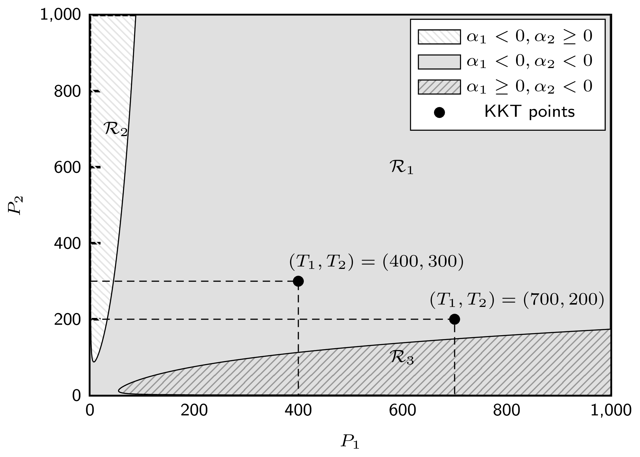
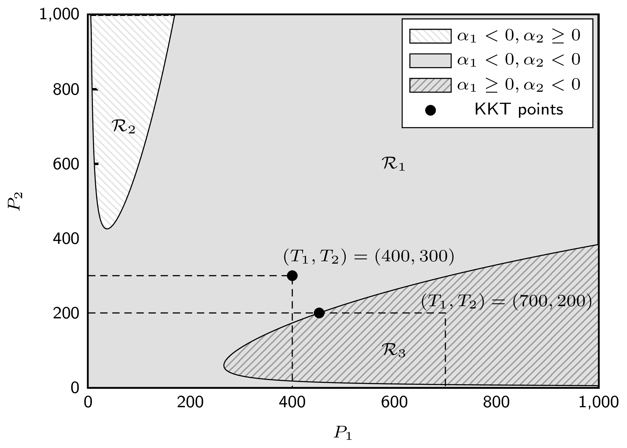
Figure 2: Example of the three feasible regions defined according to the sign of the gradient vectors for the two-user SIMO MAC with a correlation factor $\rho=0.95$ (top) and $\rho=0.99$ (bottom), for $\mathbf{h}_{1}=(1,1)^{T}$, $\mathbf{h}_{2}=(1,0.5)^{T}$ and $\sigma_{n}^{2}=1$.

Fig. 2 shows an example of the three regions described above. Each region corresponds to a different behaviour of the gradient vectors for $P_{1}$ and $P_{2}$. As observed, the boundary between $\mathcal{R}_{1}$ and $\mathcal{R}_{2}$ corresponds to the points where $\alpha_{2}(\cdot)$ is equal to zero. Similarly, the boundary between $\mathcal{R}_{1}$ and $\mathcal{R}_{3}$ corresponds to the points where $\alpha_{1}(\cdot)$ is equal to zero. Therefore, the points on both boundaries can be determined by

$$f_{1}(P_{2}, \sigma_{n}^{2},\rho,\mathbf{H})=-\frac{A}{2B\|\mathbf{h}_{1}\|^{2}\sqrt{P_{2}}}$$

$$+\sqrt{\frac{A^{2}}{4B^{2}\|\mathbf{h}_{1}\|^{4}P_{2}}+\frac{\|\mathbf{h}_{2}\|^{2}}{\|\mathbf{h}_{1}\|^{2}}P_{2}+\frac{2\sigma_{n}^{2}}{(1-\rho^{2})\|\mathbf{h}_{1}\|^{2}}},$$ (45)

$$f_{2}(P_{1}, \sigma_{n}^{2},\rho,\mathbf{H})=f_{1}(P_{1},\sigma_{n}^{2},\rho,[\mathbf{h}_{2},\mathbf{h}_{1}]),$$ (46)

where $f_{1}(\cdot)$ results from solving $\alpha_{1}(\cdot)=0$ for $\sqrt{P_{1}}$, and $f_{2}(\cdot)$ from solving $\alpha_{2}(\cdot)=0$ for $\sqrt{P_{2}}$. In this case, $f_{1}(\cdot)$ determines the values $\sqrt{P_{1}}$ where $\alpha_{1}(\cdot)=0$ for a given $P_{2}$, while $f_{2}(\cdot)$ provides the values $\sqrt{P_{2}}$ where $\alpha_{2}(\cdot)=0$ given $P_{1}$. Hence, with (45) and (46), the regions defined above can be expressed in an alternative form as

$$\mathcal{R}_{1} =\left\{(P_{1},P_{2}):\sqrt{P_{1}}\leq f_{1}(P_{2},\sigma_{n}^{2},\rho,\mathbf{H})\land\sqrt{P_{2}}\leq f_{2}(P_{1},\sigma_{n}^{2},\rho,\mathbf{H})\right\},$$ (47)

$$\mathcal{R}_{2} =\left\{(P_{1},P_{2}):\sqrt{P_{1}}\leq f_{1}(P_{2},\sigma_{n}^{2},\rho,\mathbf{H})\land\sqrt{P_{2}}>f_{2}(P_{1},\sigma_{n}^{2},\rho,\mathbf{H})\right\},$$ (48)

$$\mathcal{R}_{3} =\left\{(P_{1},P_{2}):\sqrt{P_{1}}>f_{1}(P_{2},\sigma_{n}^{2},\rho,\mathbf{H})\land\sqrt{P_{2}}\leq f_{2}(P_{1},\sigma_{n}^{2},\rho,\mathbf{H})\right\}.$$ (49)

Since the gradient cannot be equal to zero for $P_{1}$ and $P_{2}$ simultaneously, the only feasible KKT points must lie on the boundaries defined by the power constraints. In that case, we distinguish three different situations depending on the region in which the point $(\sqrt{T_{1}},\sqrt{T_{2}})$ falls into:

1. If $\left(\sqrt{T_{1}},\sqrt{T_{2}}\right)\in\mathcal{R}_{1}$, the only feasible KKT point is just $(\sqrt{T_{1}},\sqrt{T_{2}})$. On one hand, this point satisfies the KKT conditions in (39), (40), (41) and (42) with $\lambda_{1}>0$ and $\lambda_{2}>0$. On the other hand, from (47) and (48), we know that points $(t,\sqrt{T_{2}})$ with $t<\sqrt{T_{1}}$ fall into $\mathcal{R}_{1}$ or $\mathcal{R}_{2}$ where $\alpha_{1}(\cdot)$ is always negative. In this case, condition (41) forces $\lambda_{1}=0$, and (39) is no longer satisfied. The same applies to points $(\sqrt{T_{1}},t)$ where $t<\sqrt{T_{2}}$. Hence there are not more feasible KKT points on the constraints boundaries.

2. If $\left(\sqrt{T_{1}},\sqrt{T_{2}}\right)\in\mathcal{R}_{2}$, then it cannot be a KKT point because $\alpha_{2}(\cdot)>0$ in this region, and (40) cannot be satisfied with $\lambda_{2}\geq 0$. Hence, the only possible KKT point can be found by lowering the power of the second user until achieving the point that makes $\alpha_{2}(\cdot)=0$. Hence $\sqrt{P_{2}}=f_{2}(P_{1},\sigma_{n}^{2},\rho,\mathbf{H})$. In that case, the point $(\sqrt{T_{1}},f_{2}(T_{1},\sigma_{n}^{2},\rho,\mathbf{H}))$ satisfies the KKT conditions with $\lambda_{2}=0$ and $\lambda_{1}>0$.

3. By symmetry, the same reasoning applies if $\left(\sqrt{T_{1}},\sqrt{T_{2}}\right)\in\mathcal{R}_{3}$ getting $(f_{1}(T_{2},\sigma_{n}^{2},\rho,\mathbf{H}),\sqrt{T_{2}})$.

It can be concluded from the previous remarks that the feasible KKT points for the optimization problem in (35) are $\left(\sqrt{T_{1}},\sqrt{T_{2}}\right)$, $\left(\sqrt{T_{1}},f_{2}\left(\sqrt{T_{1}}\right)\right)$ and $\left(f_{1}\left(\sqrt{T_{2}}\right),\sqrt{T_{2}}\right)$, leading to the power allocations stated in the Lemma. ∎

Fig. 2 depicts a geometric representation of the KKT points depending on the shape of each region for a given channel and two different correlations, $\rho=0.95$ and $\rho=0.99$. As observed, when the power constraints are set to $(T_{1},T_{2})=(400,300)$, the corresponding point falls into $\mathcal{R}_{1}$ for both correlation factors, and hence the optimal solution allocates all the available power to both users. When the power constraints are set to $(T_{1},T_{2})=(700,200)$, the corresponding point again falls into $\mathcal{R}_{1}$ for $\rho=0.95$, but it falls into $\mathcal{R}_{3}$ for $\rho=0.99$. Thus, increasing the source correlation causes the optimal power allocation to be $(P_{1},P_{2})=(452.73,200)$. Moreover, the optimal sum-MSE for the case $(T_{1},T_{2})=(700,200)$ and $\rho=0.95$ is $\xi_{\text{sum}}^{o}=0.027$, and it decreases to $\xi_{\text{sum}}^{o}=0.010$ when $\rho=0.99$, although the power allocated to the first user is lower in the latter case. A similar result would be obtained for power constraints falling into $\mathcal{R}_{2}$, but in this case decreasing the power allocated to the second user.

In summary, using Lemma V.1 and Lemma V.2, the optimal precoders that minimize the sum-MSE for the two-user SIMO MAC are given by

• If $\rho=0$, $\rho=1$ or $|\mathbf{h}^{H}_{1}\mathbf{h}_{2}|=0$

  $$\mathbf{P}^{o}=\left[\begin{array}[]{cc}\sqrt{T_{1}}&0\\ 0&\sqrt{T_{2}}e^{-j\arg(\mathbf{h}_{1}^{H}\mathbf{h}_{2})}\end{array}\right].$$ (52)

• In any other case

  $$\mathbf{P}^{o}=\left[\begin{array}[]{cc}\min\left(\sqrt{T_{1}},f_{1}\left(T_{2}\right)\right)&0\\ 0&\min\left(\sqrt{T_{2}},f_{2}\left(T_{1}\right)\right)e^{-j\arg(\mathbf{h}_{1}^{H}\mathbf{h}_{2})}\end{array}\right].$$ (55)

Notice that combining this result with the MRT and Nu-SVD precoders described in Section III-C allows to analytically determine the gain factors $\gamma_{1}$ and $\gamma_{2}$ for the two-user MIMO MAC by simply replacing $\mathbf{h}_{k}$ by the equivalent channel responses $\tilde{\mathbf{h}}_{k}=\mathbf{H}_{k}\mathbf{u}_{k}$.

V-A Sum-MSE Analysis

In this subsection, we show some asymptotic results on the sum-MSE for the two-user MAC when optimal linear precoding is considered. We study the impact of the number of receive antennas assuming that entries of the channel matrix are i.i.d. according to a zero-mean unit-variance complex-valued Gaussian distribution, i.e., $[\mathbf{H}]_{i,j}\sim\mathcal{N}_{\mathbb{C}}(0,1)$:

• When $N_{R}\rightarrow\infty$, the sum-MSE is given by

  $$\bar{\xi}_{\text{sum}}(\sigma_{n}^{2},\rho,\mathbf{H})\approx \frac{2\sigma_{n}^{4}+(1-\rho^{2})\sigma_{n}^{2}N_{R}(T_{1}+T_{2})}{\sigma_{n}^{4}+\sigma_{n}^{2}N_{R}(T_{1}+T_{2})+T_{1}T_{2}N_{R}^{2}(1-\rho^{2})},$$

  the sum-MSE decreases when the number of receive antennas increases, since the denominator grows quadratically and the numerator linearly. Moreover, the impact of increasing the number of receive antennas on the performance varies with the source correlation. This will be checked experimentally in the results section.

• When $N_{R}=1$, the term depending on the determinant of $\mathbf{H}^{H}\mathbf{H}$ in (31) equals to zero, and we obtain the following expression for the sum-MSE

  $$\bar{\xi}_{\text{sum}}(P_{1}, P_{2},\sigma_{n}^{2},\rho,\mathbf{H})=$$

  $$\frac{2\sigma_{n}^{2}+(1-\rho^{2})(P_{1}|h_{1}|^{2}+P_{2}|h_{2}|^{2})}{\sigma_{n}^{2}+P_{1}|h_{1}|^{2}+P_{2}|h_{2}|^{2}+2\sqrt{P_{1}P_{2}}\rho|h_{1}^{H}h_{2}|}.$$ (56)

  As observed, for fixed $P_{1}$ and $P_{2}$, the impact of increasing the correlation factor $\rho$ is more significant in this case because it implies to simultaneously decrease the numerator and to increase the denominator, which contribute to lower the sum-MSE jointly. As previously shown, when $N_{R}\rightarrow\infty$, both numerator and denominator decrease with correlation.

VI Simulation Results

In this section, the performance of the precoding techniques proposed for correlated sources is evaluated for different MAC scenarios by means of computer simulations. In these simulations, $M$ vectors of $K$ source symbols are generated from a multivariate complex-valued circularly symmetric Gaussian distribution with zero mean and covariance matrix $\mathbf{C_{s}}$. Then, each user individually precodes its source symbols and transmits them over a specific realization of the fading MAC. The channel realizations are assumed to be independent and identically distributed complex-valued circularly symmetric Gaussian random variables with zero mean and unit variance, i.e., Rayleigh fading. At the receiver, each vector of observed symbols is employed to obtain an estimate of the original symbols using the corresponding linear filter. Finally, the sum-MSE between the source and the decoded symbols for the $l$-th channel realization is estimated as $\hat{\xi}^{l}_{\text{sum}}=\frac{1}{M}\sum_{m=1}^{M}\sum_{k=1}^{K}(s_{k,m}-\hat{s}_{k,m})^{2}.$ Each point of the performance curves is obtained after repeating the previous computer experiment over $L$ different channel realizations and averaging the resulting estimated sum-MSE distortions as $\hat{\xi}_{\text{sum}}=\frac{1}{L}\sum_{l=1}^{L}\hat{\xi}^{l}_{\text{sum}}.$ In particular, the different experiments consist of the transmission of blocks of $M=1000$ source symbols over $L=1000$ channel realizations. The performance indicator in the figures of this section is the sum- Signal-to-Distortion Ratio (SDR) normalized by the number of users $K$, which is defined as

$$\text{SDR (dB)}=10\log_{10}(K/\hat{\xi}_{\text{sum}}).$$ (57)

This performance indicator is usually plotted with respect to the SNR. Without loss of generality, we assume $\sigma_{n}^{2}=1$ and, therefore, the SNR per user is directly given by its power constraint: $\text{SNR}_{k}~{}\text{(dB)}=10\log_{10}(T_{k})~{}\forall k$.

In this section, we present the performance of the proposed linear precoding schemes in terms of the obtained SDR for different ranges of SNR. We also plot an upper bound for the achievable SDR under the assumption of separate source and channel coding, whose computation is described in Appendix A. Also, in some scenarios we show the performance of a transmission scheme that uses non-linear modulo functions to transform the source symbols [7], prior to being encoded with the linear strategies described in this work. In this case, the modulo mappings are optimized for the equivalent channel matrix resulting from the product of precoding and channel. Note that this approach can be seen as a scheme that separately performs non-linear source encoding and linear channel encoding. This strategy helps to gain some insight on the differences observed with respect to the separation bound.

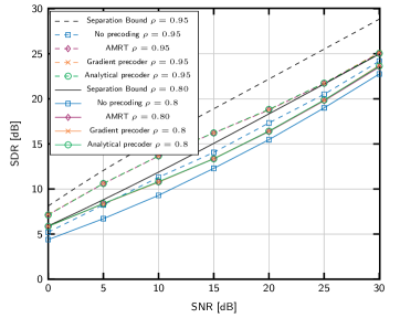
Figure 3: Performance with and without precoding for a two-user SIMO MAC with $N_{R}=2$ receive antennas and equal power constraints. Two different correlation factors are considered: $\rho=0.8$ and $\rho=0.95$.

In the first computer experiment, we consider a two-user SIMO MAC scenario with $N_{R}$ = 2 receive antennas. The power constraints are identical for the two users, i.e. $\text{SNR}_{1}=\text{SNR}_{2}=\text{SNR}$, and $\rho$ is the correlation between the two users symbols. Fig. 3 shows the performance curves obtained when the source symbols are transmitted with the analytical precoder given by (55) for two different correlation factors: $\rho=0.8$ and $\rho=0.95$. These curves are compared to those obtained with other three approaches: 1) scaling by the available powers (i.e. without precoding), 2) low-complexity AMRT in Section III-B, and 3) the projected gradient algorithm described in Section III-A. On one hand, the optimal linear precoder provides a performance gain for all range of SNRs with respect to no precoding, especially for low and medium SNRs. As expected, this gain is larger for higher correlation factors, since it ranges between $0.7$ dB and $1.6$ dB for $\rho=0.8$, and between $1$ dB and $2.5$ dB for $\rho=0.95$. On the other hand, the AMRT and the projected gradient algorithms provide the same performance as that of the optimal precoder. Note that AMRT and no precoding allocate all the available power to both user. Thus the gain of the AMRT with respect to no precoding comes just from adjusting the phase of the encoder coefficients. Also, for the two-user SIMO MAC, the phase computed by AMRT agrees with the optimal one. According to the AMRT definition in (10) and assuming, without loss of generality, that $\mathbf{g}=\lambda\mathbf{h}_{1}$, the scalar gains are $p_{1}=\frac{\sqrt{T_{k}}}{\|\mathbf{h}_{1}^{H}\mathbf{g}\|}\mathbf{h}_{1}^{H}\mathbf{g}=\sqrt{T_{1}}$ and $p_{2}=\frac{\sqrt{T_{k}}}{\|\mathbf{h}_{2}^{H}\mathbf{g}\|}\mathbf{h}_{2}^{H}\mathbf{g}=\frac{\sqrt{T_{k}}}{\|\mathbf{h}_{2}^{H}\mathbf{h}_{1}\|}\mathbf{h}_{2}^{H}\mathbf{h}_{1}$, and we can see that they comply with the optimality condition in (33). We then conclude that in this scenario with equal power constraints, the gain comes mainly from an appropriate adjusting of the encoder phases. Finally, the gap with respect to the separation bound is especially small for low SNRs, although it gradually increases with the SNR.

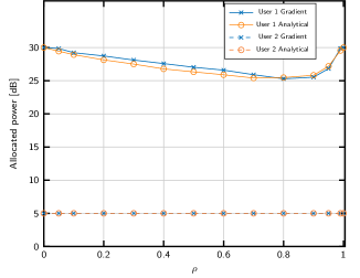
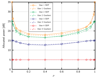
Figure 4: Average power allocated to each user after precoding the source symbols for a two-user SIMO MAC with $N_{R}=2$ antennas when the power constraints are set such that $\text{SNR}_{1}=30$ dB and $\text{SNR}_{2}=5$ dB (top). Four-user SISO MAC with $N_{R}=1$ antennas and power constraints $\text{SNR}=[35,25,15,5]$ (bottom).

Fig. 4 plots the average power allocated to each user depending on the source correlation for two scenarios: 1) a two-user SIMO MAC with $N_{R}=2$ antennas, when the individual power constraints are set such that $\text{SNR}_{1}=30$ dB and $\text{SNR}_{2}=5$ dB, 2) a four-user MAC with $N_{T}=1$ and $N_{R}=1$ antennas, and power constraints such that the user SNRs are 35, 25, 15 and 5 dB. The optimal precoders in the first scenario are obtained, for each channel realization, using the analytical expression in (55) and the projected gradient algorithm explained in Section III-A. Then, the power allocated to each user is averaged over all channel realizations. As observed, the user with the most restrictive power constraint transmits at its maximum power to lower the sum-MSE. The power allocated to the other user depends on the correlation factor. As explained in Section V, this power is the maximum available when the correlation factor is $\rho=0$ and $\rho=1$. However, the users with the largest power budgets should not use all their available power for intermediate correlation factors. In the second scenario, the linear precoders are obtained with the semidefinite relaxation described in Section IV and also with the gradient algorithm. The results suggest that the optimal power allocation policy for this scenario is similar to that of the previous case, and the users with more available power can benefit from the source correlation to save power for a broad range of correlation factors. This also justifies the approach proposed in Section III-C, which is based on the assumption that allocating all the available power to the users is not necessarily optimal when $\rho>0$.

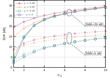
Figure 5: Performance of the optimal linear precoder depending on the number of receive antennas for the two-user SIMO MAC, for SNR=5 dB and SNR=20 dB, and different correlation factors.

Fig. 5 shows the performance of the optimal linear precoder for the two-user SIMO MAC with a different number of receive antennas, for SNR=5 dB and SNR=20 dB. Separation bounds are omitted for clarity. An interesting result is observed when the source symbols are highly correlated since high SDR values are obtained even for a small number of receive antennas. As seen in (56), the phase of the user precoders is designed to exploit the source correlation by aligning the user channels, which contributes to lower the sum-MSE, especially for $N_{R}=1$ and high correlation factors. The impact of increasing the receive antennas on the SDR is more remarkable for uncorrelated sources, although the performance gain diminishes for a large number of receive antennas regardless of the source correlation. Moreover, the gain due to the correlation with a large number of receive antennas vanishes for high SNRs, while a small gain is still observed for low SNRs. This agrees with the asymptotic analysis shown in Section III.

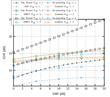
Figure 6: Performance with different precoding strategies for a SIMO MAC with and without precoding depending on the number of receive antennas $N_{R}$ with $K=10$ users, $\rho=0.95$ and equal power constraints.

We now consider a SIMO MAC scenario with $K=10$ users. In such a case, the optimal sum-MSE precoders cannot be obtained via analytical expressions. Hence, we show results for the projected gradient algorithm, the SDP in Section IV, and the aligned MRT algorithm in Section III-B. Fig. 6 shows the performance curves with and without precoding for three different number of receive antennas: $N_{R}=1$, $2$ and $5$. The power constraints are equal for all the users and the source correlation is $\rho_{i,j}=\rho=0.95,\forall i\neq j$. The corresponding bounds based on source-channel separation are also shown. As observed, the performance achieved by the AMRT and the SDP is close to the one provided by the projected gradient algorithm. The gain provided by these precoders is more significant as the number of receive antennas is smaller, and the extreme case occurs when $N_{R}=1$ where the precoding gain is substantial (about $8$ dB). Increasing the number of receive antennas improves the overall performance in general, but the gain provided by the different precoders is not so significant with respect to the uncoded case. These results agree with the behavior observed for two users and confirm the suitability of linearly encoding the source symbols for scenarios with a smaller number of receive antennas than users and correlated sources. It is also interesting to remark that for low SNR values, the precoding schemes improve the bound based on source-channel separation, showing that some low computational complexity strategies such as AMRT can beat separate coding.

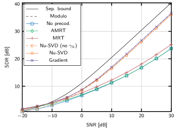
Figure 7: Performance with different precoding strategies for a MIMO MAC with $K=10$, $N_{T}=2$, $N_{R}=10$, $\rho=0.40$ and equal power constraints.

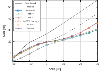
Figure 8: Performance with different precoding strategies for a MIMO MAC with $K=10$, $N_{T}=2$, $N_{R}=10$, $\rho=0.99$ and equal individual constraints.

In the ensuing experiments, we consider a MIMO MAC scenario with $K=10$ users with $N_{T}=2$ antennas per user and equal power constraints, and a receiver with $N_{R}=10$ antennas. The correlation factor is $\rho_{{i,j}}=\rho=0.40~{}\forall i,j,~{}i\neq j$. Figure 7 plots the performance curves when the linear precoder is obtained with the following strategies: 1) projected gradient algorithm, 2) AMRT, 3) optimized MRT, 4) optimized Nu-SVD and 5) Regular Nu-SVD. Recall that for the optimized version of MRT and Nu-SVD, the factor gains $\gamma_{k}$ are adjusted as explained in Section III-C to exploit the source correlation. At the receiver, the linear MMSE filter, given by (4), is employed for all the precoding methods. On one hand, the precoder obtained with the projected gradient algorithm provides the best performance for all the considered SNR values. The optimized Nu-SVD scheme closely approaches this performance for all SNR values, providing certain gain (about 1-2 dB) with respect to the regular Nu-SVD up to SNR=0 dB, due to the adjusting of the factor gains. Optimized MRT also obtains the same performance as the gradient precoder and Nu-SVD for SNR values below 0 dB, but the gap with the other strategies increases with the SNR. Low-complexity AMRT behaves in a similar way to the previous strategies at low SNR regimes, but it converges to the uncoded scheme for SNR $\geq 0$ dB since the correlation between the source symbols is low. On the other hand, projected gradient and Nu-SVD performance stay close to the separation bound, due to the low correlation factor, while the modulo-based encoding of the source symbols does not contribute to improving the performance. Also, the separation bound shown for $K>2$ users does not take into account individual constraints and the bound calculation is only based on equating the sum-distortion and the sum-capacity. For this reason, the separation bound is not necessarily tight and an additional gap between the performance curves and the bound can be observed. In spite of that, linear precoder exceeds the performance of any separation-based scheme in the low SNR regime.

Fig. 8 plots the performance curves for the previous scenario but for higher correlation $\rho=0.99$. Again, the best performance is achieved with the precoders obtained with the projected gradient algorithm, and the optimized Nu-SVD precoding scheme also performs closely for all SNR values. In this case, adjusting the $\gamma_{k}$ factors significantly improves the SDR obtained with the regular Nu-SVD (about $5$ dB for low SNRs) due to the higher source correlation. MRT also takes advantage of the high correlation and performs close to those schemes for SNRs below $10$ dB, lowering the gap for high SNRs with respect to $\rho=0.4$. Similar behavior is observed for AMRT, although for large SNR values its performance is again closer to no precoding. In this scenario, the gap with respect to the separation bound is larger than in the previous experiment. It is interesting to observe that, unlike for $\rho=0.4$, the combination of modulo mappings and linear precoding provides significant improvement with respect to directly precoding the source information, especially for high SNRs. This combined strategy allows to reduce the gap to the separation bound for SNR values over 0 dB, and this gain can be attributed to the non-linear nature of the modulo mapping. Different works [2, 9] have shown that the linear precoder of source symbols is optimal for SNRs lower than a particular value. However, this SNR threshold diminishes as the source correlation increases and, in this case, non-linear mappings are required to approach the theoretical limits.

VII Conclusion

Linear distributed encoding for the transmission of correlated information over fading MIMO MACs has been considered. Precoders are designed to minimize the sum-MSE considering the source correlation which results in a non-convex optimization problem. We have proposed different strategies to obtain the linear precoders at each user in the general MIMO MAC scenario. The convergence of these solutions to the optimal minimum is not guaranteed, but they provide good performance in different situations and various computational complexity levels. In the more restrictive case of two-user SIMO MAC, we have derived a closed-form expression for the optimal precoder. A significant performance gain is achieved by adjusting the precoder phase difference between the two nodes and with an adequate power allocation. Regarding power allocation, an interesting fact has been observed: the nodes must transmit with all the available power when sources are either uncorrelated and fully correlated, while for other correlation levels lower power can be used. Computer simulations show a significant performance improvement regarding SDR with respect to the uncoded case, especially for low SNRs and numbers of transmitting nodes larger than the number of receive antennas, where it is possible to achieve large SDR values by exploiting the source correlation. Hence, the proposed strategies are useful in those communication scenarios such as WSNs, where the simplicity and the power consumption of the nodes is a critical requirement.

Appendix A Upper Bound based on Source-Channel Separation

The separation bound is calculated by equating the source rate-distortion region and the capacity region of the fading MAC. Given a set of distortion targets $\mathbf{d}=[D_{1},D_{2},...,D_{N}]^{T}$, the rate distortion region $\mathcal{R}(\mathbf{d})$ is the set of rate distortion functions corresponding to the individual sources, i.e. $R_{k}^{D}(D_{i}),k=1,...,K$, and by the sum-rate distortion function $R_{\text{sum}}^{D}(\mathcal{D})$. For the case of distributed encoding of bivariate Gaussian sources under the MSE distortion, this region is defined in [33, 34]. For scenarios with more than two source symbols, [35] provides the following lower bound for the sum-rate

$$R_{\text{sum}}^{D}(\mathbf{d})=\min_{\mathbf{D}_{\mathbf{s}}:d_{ii}\leq[\mathbf{d}]_{i}}~{}~{}\log\left(\frac{|\mathbf{C}_{\mathbf{s}}|}{|\mathbf{D}_{\mathbf{s}}|}\right),$$ (58)

where $\mathbf{D}_{\mathbf{s}}=(\mathbf{C}_{s}^{-1}+\mathbf{B})^{-1}$, for some diagonal matrix $\mathbf{B}$, and $\mathbf{C}_{\mathbf{s}}$ is the source covariance matrix. The whole rate-distortion region is defined by (58) applied to all user subsets, but its computation is unaffordable for large number of users. In this case, the separation bound can be approximated by equating only the sum-distortion function to the sum-capacity of the MAC. In general, this bound will be optimistic since the individual rate constraints are not necessarily satisfied.

The sum-capacity of a MIMO MAC with non-cooperative users is

$$R_{\text{{sum}}}^{C}(\mathbf{H})=\log\left|\mathbf{I}+\frac{1}{\sigma_{n}^{2}}\sum_{k=1}^{K}\mathbf{H}_{k}\mathbf{Q}_{k}\mathbf{H}_{k}^{H}\right|,$$ (59)

where the covariance matrices $\mathbf{Q}_{k}$ can be computed with the iterative waterfilling algorithm [36], with the constraints $\operatorname{tr}(\mathbf{Q}_{k})<T_{k},\forall k$.

In general, the separation bound can be defined in terms of intersections between the rate distortion and capacity regions. For two users, we state the following minimization problem

$$D_{\text{sum}}(\mathbf{H})=\min_{D_{1},D_{2}:\mathcal{C}(\mathbf{H})\cap\mathcal{R}(D_{1},D_{2})\neq\emptyset}~{}~{}D_{1}+D_{2},$$ (60)

where $\mathcal{C}(\mathbf{H})$ represents the capacity region while $\mathcal{R}(D_{1},D_{2})=\mathcal{R}_{1}^{D}(D_{1})\cap\mathcal{R}_{2}^{D}(D_{2})\cap\mathcal{R}_{\text{sum}}^{D}(D_{1},D_{2})$ is the corresponding rate distortion region for the bivariate Gaussian distribution. For $K>2$, we will only consider the constraints on the sum rates for all users, due to the computational complexity of searching for the best intersection between regions in such case. Hence, the separation bound is calculated by equating (58) and (59), i.e.,

$$D_{\text{sum}}(\mathbf{H})=\min_{\mathbf{d}:R^{D}_{\text{sum}}(\mathbf{d})=R_{\text{sum}}^{C}(\mathbf{H})}~{}~{}\mathbf{1}^{T}\mathbf{d},$$ (61)

and then averaging the obtained distortions for each channel realization to determine the optimum SDR, i.e. $\text{SDR}_{\text{opt}}=\mathbb{E}_{\mathbf{H}}[1/D_{\text{sum}}(\mathbf{H})].$

References

- [1] C. E. Shannon, “A mathematical theory of communication,” The Bell System Technical Journal, vol. 7, pp. 379–423, 1948.
- [2] A. Lapidoth and S.Tingueley, “Sending a bivariate Gaussian over a Gaussian MAC,” IEEE Trans. on Information Theory, vol. 56, no. 6, pp. 2714–2752, 2010.
- [3] D. Gunduz, E. Erkip, A. Goldsmith, and V. Poor, “Source and channel coding for correlated sources over multiuser channels,” IEEE Trans. on Information Theory, vol. 55, no. 9, pp. 3927–3944, Sep 2009.
- [4] K.-H. Lee and D. Petersen, “Optimal linear coding for vector channels,” IEEE Transactions on Communications, vol. 24, no. 12, pp. 1283–1290, Dec 1976.
- [5] J. Karlsson and M. Skoglund, “Lattice-based source-channel coding in wireless sensor networks,” in 2011 IEEE International Conference on Communications (ICC), June 2011, pp. 1–5.
- [6] M. S. Mehmetoglu, E. Akyol, and K. Rose, “Deterministic annealing-based optimization for zero-delay source-channel coding in networks,” IEEE Transactions on Communications, vol. 63, no. 12, pp. 5089–5100, Dec 2015.
- [7] P. Suárez-Casal, O. Fresnedo, L. Castedo, and J. García-Frías, “Analog transmission of correlated sources over fading simo multiple access channels,” IEEE Transactions on Communications, vol. 65, no. 7, pp. 2999–3011, July 2017.
- [8] N. Wernersson, J. Karlsson, and M. Skoglund, “Distributed quantization over noisy channels,” IEEE Transactions on Communications, vol. 57, no. 6, pp. 1693–1700, June 2009.
- [9] P. A. Floor, A. N. Kim, T. A. Ramstad, I. Balasingham, N. Wernersson, and M. Skoglund, “On joint source-channel coding for a multivariate gaussian on a gaussian mac,” IEEE Transactions on Communications, vol. 63, no. 5, pp. 1824–1836, May 2015.
- [10] N. Wernersson and M. Skoglund, “Nonlinear coding and estimation for correlated data in wireless sensor networks,” IEEE Transactions on Communications, vol. 57, no. 10, pp. 2932–2939, October 2009.
- [11] M. Costa, “Writing on dirty paper (corresp.),” IEEE Transactions on Information Theory, vol. 29, no. 3, pp. 439–441, May 1983.
- [12] M. Tomlinson, “New automatic equaliser employing modulo arithmetic,” Electronics Letters, vol. 7, no. 5, pp. 138–139, March 1971.
- [13] H. Harashima and H. Miyakawa, “Matched-transmission technique for channels with intersymbol interference,” IEEE Transactions on Communications, vol. 20, no. 4, pp. 774–780, Aug 1972.
- [14] Q. H. Spencer, A. L. Swindlehurst, and M. Haardt, “Zero-forcing methods for downlink spatial multiplexing in multiuser mimo channels,” IEEE Transactions on Signal Processing, vol. 52, no. 2, pp. 461–471, Feb 2004.
- [15] Z. Pan, K.-K. Wong, and T.-S. Ng, “Generalized multiuser orthogonal space-division multiplexing,” IEEE Transactions on Wireless Communications, vol. 3, no. 6, pp. 1969–1973, Nov 2004.
- [16] M. Schubert and H. Boche, “Solution of the multiuser downlink beamforming problem with individual sinr constraints,” IEEE Transactions on Vehicular Technology, vol. 53, no. 1, pp. 18–28, Jan 2004.
- [17] R. Hunger, M. Joham, and W. Utschick, “On the mse-duality of the broadcast channel and the multiple access channel,” IEEE Transactions on Signal Processing, vol. 57, no. 2, pp. 698–713, Feb 2009.
- [18] A. J. Tenenbaum and R. S. Adve, “Joint multiuser transmit-receive optimization using linear processing,” in 2004 IEEE International Conference on Communications (IEEE Cat. No.04CH37577), vol. 1, June 2004, pp. 588–592.
- [19] S. Shi, M. Schubert, and H. Boche, “Downlink mmse transceiver optimization for multiuser mimo systems: Mmse balancing,” IEEE Transactions on Signal Processing, vol. 56, no. 8, pp. 3702–3712, Aug 2008.
- [20] J. González-Coma, A. Gründinger, M. Joham, and L. Castedo, “MSE Balancing in the MIMO BC: Unequal Targets and Probabilistic Interference Constraints,” IEEE Transactions on Signal Processing, vol. PP, no. 99, pp. 1–1, 2017.
- [21] O. Dabeer, A. Roumy, and C. Guillemot, “Linear transceivers for sending correlated sources over the gaussian mac,” in National Communication Conference, Kanpur (India), Jan 2007.
- [22] J. Yang and A. Swindlehurst, “Maximum sinr beamforming for correlated sources,” in 1995 International Conference on Acoustics, Speech, and Signal Processing, vol. 3, May 1995, pp. 1916–1919 vol.3.
- [23] J. Acharya, R. Roy, J. Singh, and C. Rose, “Optimal signature sets for transmission of correlated data over a multiple access channel,” in Global Telecommunications Conference, 2004. GLOBECOM ’04. IEEE, vol. 2, Nov 2004, pp. 1046–1050 Vol.2.
- [24] P. Yahampath, “Steepest-descent optimization of cdma signatures for multiple correlated sources with applications to joint source-channel coding,” IEEE Transactions on Communications, vol. 63, no. 4, pp. 1343–1354, April 2015.
- [25] S. M. Kay, Fundamentals of Statistical Signal Processing. Prentice Hall, 1993.
- [26] T. L. Marzetta, “Noncooperative Cellular Wireless with Unlimited Numbers of Base Station Antennas,” IEEE Transactions on Wireless Communications, vol. 9, no. 11, pp. 3590–3600, November 2010.
- [27] D. Bertsekas, “On the goldstein-levitin-poljak gradient projection method,” IEEE Trans. on Automatic Control, vol. 52, no. 2, pp. 461–471, Feb 2004.
- [28] E. Björnson, M. Bengtsson, and B. Ottersten, “Optimal Multiuser Transmit Beamforming: A Difficult Problem with a Simple Solution Structure [Lecture Notes],” Signal Processing Magazine, IEEE, vol. 31, no. 4, pp. 142–148, July 2014.
- [29] T. Bogale and L. Vandendorpe, “Robust Sum MSE Optimization for Downlink Multiuser MIMO Systems With Arbitrary Power Constraint: Generalized Duality Approach,” IEEE Transactions on Signal Processing, vol. 60, no. 4, pp. 1862–1875, April 2012.
- [30] A. Beck and M. Teboulle, “On minimizing quadratically constrained ratio of two quadratic functions,” Journal of Convex Analysis, vol. 17, no. 3, pp. 789–804, 2010.
- [31] W.Karush, “Minima of functions of several variables with inequalities as side constraints,” M.Sc. Dissertation, Dept. of Mathematics, Univ. of Chicago, Chicago, Illinois,, 1939.
- [32] H. W. Kuhn and A. W. Tucker, “Nonlinear programming,” in Proc. of 2nd Berkeley Symposium. Berkeley: University of California Press, 1951, pp. 481–492.
- [33] Y. Oohama, “Gaussian multiterminal source coding,” vol. 43, no. 6, pp. 1912–1923, Nov 1997.
- [34] A. Wagner, S. Tavildar, and P. Viswanath, “Rate region of the quadratic Gaussian two-encoder source-coding problem,” vol. 54, no. 5, pp. 1938–1961, May 2008.
- [35] J. Wang, J. Chen, and X. Wu, “On the Sum Rate of Gaussian Multiterminal Source Coding: New Proofs and Results,” IEEE Transactions on Information Theory, vol. 56, no. 8, pp. 3946–3960, Aug 2010.
- [36] W. Yu, W. Rhee, S. Boyd, and J. M. Cioffi, “Iterative water-filling for gaussian vector multiple-access channels,” IEEE Transactions on Information Theory, vol. 50, no. 1, pp. 145–152, Jan 2004.