Traversable Wormholes in Minimally Geometrical Deformed
Trace-Free Gravity using Gravitational Decoupling

Abstract

In this work, we investigate wormhole solutions through the utilization of gravitational decoupling, employing the Minimal Geometric Deformation (MGD) procedure within the framework of Trace-Free Gravity. We base our investigation on static and spherically symmetric Morris-Thorne traversable wormholes, considering both constant and variable equation of state parameters. We derive the field equations and extract the shape function for each scenario. Moreover, we explore the gravitational decoupling technique and examine various forms of energy density for both a smeared and particle-like gravitational source, encompassing the realm of noncommutative geometry and a statically charged fluid. We also examinethe wormhole geometry through the utilization of embedding diagrams. Through our analysis, we uncover a violation of the Null Energy Condition (NEC). To conclude, we employ the Gauss-Bonnet theorem to determine the weak deflection angle for the wormhole configurations.

I Introduction

A Trace-Free version of the Einstein (TFE) equations provides the resolution of the cosmological constant problem of which the observed cosmological constant is much smaller than the expected value. The formulation was proposed by Weinberg in his review Weinberg:1988cp . Indeed, the trace-free gravity is essentially equivalent to adopting unimodular gravity Finkelstein:2000pg ; Henneaux:1989zc ; Unruh:1988in ; Ng:1990xz ; Alvarez:2005iy ; Ellis:2010uc ; Ellis:2013uxa ; Barcelo:2014mua ; Burger:2015kie ; Alvarez:2015oda ; Shaposhnikov:2008xb ; Smolin:2010iq ; Jain:2012gc ; Alvarez:2013fs ; Eichhorn:2013xr and its generalized versions Barvinsky:2019agh ; Barvinsky:2017pmm . The approach does not only determine a unique value for the effective cosmological constant, but it also does solve the discrepancy between theory and observation in the standard approach. This article is aimed to investigate traversable wormhole solutions in TFE gravity, incorporating the consideration of variable equations of state and taking advantage of gravitational decoupling by means of minimal geometric deformation (MGD) approach.

As widely acknowledged, solving Einstein field equations poses a non-trivial challenge, particularly when dealing with cases invoking spherical symmetry. A recent advancement addressing this complexity is the introduction of a novel methodology known as the gravitational decoupling through the minimal geometric deformation (MGD) scheme Ovalle:2017fgl ; Ovalle:2017wqi . The Brane-World scenario Casadio:2012rf ; Casadio:2013uma ; Ovalle:2013xla ; Ovalle:2014uwa ; Casadio:2015jva was originally investigated using such an approach. Subsequently, it evolved into a gravitational source decoupling scheme, facilitating the extension of isotropic spherical solutions of the Einstein field equations to encompass anisotropic domains Ovalle:2017fgl . Over time, this approach has been broadly adopted across various branches, see for wormholes Tello-Ortiz:2021kxg , playing a pivotal role in expanding or constructing novel solutions for the Einstein equations and their extensions, see e.g., Casadio:2015gea ; Ovalle:2017wqi ; Ovalle:2018gic ; Tello-Ortiz:2022hyf .

Gibbons and Werner introduced a novel geometric approach for computing the weak deflection angle, employing the Gauss-Bonnet theorem (GBT) on optical geometries applicable to asymptotically flat spacetimes Gibbons:2008rj . This technique involves solving the GBT integral over an infinite domain defined by the light ray boundaries. Subsequently, Werner extended this methodology to stationary spacetimes by incorporating the Finsler-Randers optical geometry, utilizing Nazım’s osculating Riemannian manifolds Werner:2012rc .

Building upon Werner’s work, Ishihara et al. further extended the method to finite distances, specifically considering scenarios with significant impact parameters, as opposed to relying on asymptotic receiver and source conditions Ishihara:2016vdc ; Ishihara:2016sfv . T. Ono et al. later applied this finite-distance approach to axisymmetric spacetimes Ono:2017pie . Crisnejo and Gallo Crisnejo:2018uyn utilized the GBT to derive gravitational light deflections within a plasma medium. More recently, Li et al. investigated the impact of finite distances on the weak deflection angle, introducing massive particles and the Jacobi metric within the framework of GBT Li:2020dln ; Li:2020wvn . For further developments in this field, one can refer to more recent works on wormholes Jusufi:2017mav ; Ovgun:2018tua ; Ovgun:2018fnk ; Kumaran:2021rgj and black holes Javed:2022kzf ; Pantig:2022toh ; Okyay:2021nnh ; Belhaj:2020rdb ; Islam:2020xmy ; Kumar:2020hgm ; QiQi:2023nex ; Huang:2023bto ; dePaula:2023ozi ; Huang:2022gon ; Huang:2022soh ; Parbin:2022iwt ; Halla:2022xce .

In this work, we investigate wormhole solutions through the utilization of gravitational decoupling, employing the MGD procedure within the framework of Unimodular Gravity. In Sec.II, we take a recap of the basic concept of Unimodular Gravity and employ the MGD procedure. We then examine static and spherically symmetric Morris-Thorne traversable wormholes in Sec.III. In this section, we consider both constants and variables in the equation of state parameter. We also compute the shape function for each case. In Sec.IV, we consider the gravitational decoupling technique and consider the forms of the energy density for a gravitational source in the context of noncommutative geometry and a statically charged fluid. Here we obtain the decoupled solutions of the wormholes. Moreover, we test the energy conditions. Subsequently, the embedding diagrams of the wormholes are illustrated in Sec.V. In Sec.VII, we use the Gauss-Bonnet theorem to compute the weak deflection angle for wormhole solutions. We conclude our findings in the last section.

II Unimodular Gravity & Its Geometrical Deformation

A detailed formulation of trace-free Einstein gravity and its relationship with unimodular gravity is given in Refs.Ellis:2010uc ; Ellis:2013uxa . Recall that in the standard formulation the gravitational field is governed by the Einstein field equations:

$$R_{\mu\nu}-\frac{1}{2}g_{\mu\nu}R+\lambda g_{\mu\nu}=8\pi T^{(m)}_{\mu\nu}\,.$$ (1)

As a result, in unimodular gravity, the presence of an additional constraint on the metric determinant reduces $10$ independent field equations to $9$ independent field equations. Taking the trace of the field equations (1), we obtain

$$4\lambda=R+8\pi T^{(m)}\,.$$ (2)

Multiplying each side of Eq.(2) by $\tfrac{1}{4}g_{\mu\nu}$ and adding the result to Eq.(1) yields the trace-free field equations:

$$G_{\mu\nu}=8\pi{\bar{T}}_{\mu\nu}\,,$$ (3)

where we have defined

$$G_{\mu\nu}\equiv R_{\mu\nu}-\frac{1}{4}g_{\mu\nu}R\,,$$ (4)

and

$${\bar{T}}_{\mu\nu}\equiv\left(T^{(m)}_{\mu\nu}-\frac{1}{4}g_{\mu\nu}T^{(m)}\right)\,.$$ (5)

Any extension to the above theory will eventually produce new terms in the effective four-dimensional Einstein equations. These “corrections” are usually handled as part of an effective energy-momentum tensor. In the following, the MGD takes the simplest modification:

$$G_{\mu\nu}=8\pi{\bar{T}}_{\mu\nu}+\delta({\rm new\,\,terms})_{\mu\nu}\,,$$ (6)

The new terms in Eq.(6) may be viewed as part of an effective energy-momentum tensor, whose explicit form may contain new fields, like scalar, vector, and tensor fields, all of them coming from the new gravitational sector not described by Einstein’s theory.

Therefore, we have the following modification to the stress-momentum tensor:

$$T_{\mu\nu}={\bar{T}}_{\mu\nu}+\alpha({\rm new\,\,terms})_{\mu\nu}=\Big{(}T^{(m)}_{\mu\nu}-\frac{1}{4}g_{\mu\nu}T^{(m)}\Big{)}+\delta\,\varepsilon_{\mu\nu}\,.$$ (7)

It is clear that the case $\delta=0$ yields to the original Unimodular Gravity. We consider the contribution of two gravitational sources $T^{\mu(m)}_{\nu}$, which is known as the seed source and $\varepsilon^{\mu}_{\nu}$. Here the intensity of influence of the source $\varepsilon_{\mu\nu}$ over $T^{(m)}_{\mu\nu}$ parametrized by a dimensionaless constant $\delta$.

III Traversable Wormhole Solutions

We consider a static and spherically symmetric Morris-Thorne traversable wormhole in the Schwarzschild coordinates $(t,r,\theta,\phi)$ given by [4]

$$ds^{2}=-e^{2\Phi(r)}dt^{2}+\frac{1}{\left(1-\frac{b(r)}{r}\right)}dr^{2}+r^{2}\left(d\theta^{2}+\sin^{2}\theta d\phi^{2}\right)\,,$$ (8)

where $\Phi(r)$ and $b(r)$ are the redshift and shape functions, respectively. They are functions of the radial coordinate $r$ only. In the wormhole geometry, the redshift function $\Phi$ should be finite in order to avoid the formation of an event horizon. The radial coordinate $r$ ranges from a minimum value $r_{0}$, corresponding to the throat of the wormhole, where $b(r_{0})=r_{0}$ at $r=r_{0}$. A crucial aspect of wormholes is the flaring-out condition, expressed as $b(r)-b^{\prime}(r)r\geq 0$ in the vicinity of the throat, where a prime denotes a derivative with respect to the radial coordinate $r$. Additionally, it is required that $b(r)/r\rightarrow 0$ as $r\rightarrow\infty$. It is worth noting that the supplementary condition $b(r)/r<1$ is also enforced. We define a perfect fluid source with energy-momentum tensor as

$${\bar{T}}_{ab}=({\bar{\rho}}+{\bar{p}}_{t})U_{a}U_{b}+{\bar{p}}_{t}g_{ab}+({\bar{p}}_{r}-{\bar{p}}_{t})X_{a}X_{b}\,,$$ (9)

where $\bar{\rho}$ is the energy density measured by a comoving observer with the fluid, and $U_{a}$ and $X_{a}$ are its timelike four-velocity and a spacelike unit vector orthogonal to $U_{a}$ and angular directions, respectively. We define an appropriate frame of the fluid velocity vectors Cadoni:2020izk

$$U^{a}=e^{-\Phi}\delta^{a}_{0}\,,\quad X^{a}=\sqrt{1-\frac{b(r)}{r}}\delta^{a}_{1}\,,$$ (10)

so that $U_{a}U^{a}=-1$ and $X_{a}X^{a}=1$. Here we are working in geometrized units setting the gravitational constant $G$ and the speed of light $c$ to unity. The trace-free components of the energy-momentum tensor Eq.(9) in this case read

$${\bar{T}}_{ab} = \biggl{(}\frac{1}{4}e^{2\Phi}\left({\bar{p}}_{r}+2{\bar{p}}_{t}+3{\bar{\rho}}\right),\frac{1}{4}(3{\bar{p}}_{r}-2{\bar{p}}_{t}+{\bar{\rho}})\frac{1}{(1-\frac{b}{r})},$$ (11)

$$\quad\quad\frac{1}{4}r^{2}\left(-{\bar{p}}_{r}+2{\bar{p}}_{t}+{\bar{\rho}}\right),\frac{1}{4}r^{2}\sin^{2}(\theta)\left(-{\bar{p}}_{r}+2{\bar{p}}_{t}+{\bar{\rho}}\right)\biggl{)}.$$

For $(t,t)$ component, we find

$${\cal G}_{tt}=\frac{e^{2\Phi}}{4r^{2}}(b^{\prime}(2-r\Phi^{\prime})+2r(2\Phi^{\prime}+r\Phi^{\prime 2}+r\Phi^{\prime\prime})-b(3\Phi^{\prime}+2r\Phi^{\prime 2}+2r\Phi^{\prime\prime})),$$ (12)

while for $(r,r)$ component,

$${\cal G}_{rr}=\frac{1}{4(b-r)r^{2}}(b(4+5r\Phi^{\prime}-2r^{2}\Phi^{\prime 2}-2r^{2}\Phi^{\prime\prime})+r(-b^{\prime}(2+r\Phi^{\prime})+2r(-2\Phi^{\prime}+r\Phi^{\prime 2}+r\Phi^{\prime\prime}))),$$ (13)

and for $(\theta,\theta)$ component,

$${\cal G}_{\theta\theta}=\frac{1}{4r}(b(2+r\Phi^{\prime}-2r^{2}\Phi^{\prime 2}-2r^{2}\Phi^{\prime\prime})+r^{2}(-b^{\prime}\Phi^{\prime}+2r(\Phi^{\prime 2}+\Phi^{\prime\prime}))),$$ (14)

where ${\cal G}_{\theta\theta}=\sin^{2}\theta{\cal G}_{\phi\phi}$. Then using the information of metric (4) and (5) in the TFE for the general form, we come up with

$$8\pi\left[\left({\bar{p}}_{r}+2{\bar{p}}_{t}+3{\bar{\rho}}\right)\right] = \frac{1}{r^{2}}(b^{\prime}(2-r\Phi^{\prime})+2r(2\Phi^{\prime}+r\Phi^{\prime 2}+r\Phi^{\prime\prime})$$ (15)

$$-b(3\Phi^{\prime}+2r\Phi^{\prime 2}+2r\Phi^{\prime\prime}))\,,$$

$$8\pi\left[(3{\bar{p}}_{r}-2{\bar{p}}_{t}+{\bar{\rho}})\right] = \frac{-1}{r^{3}}(b(4+5r\Phi^{\prime}-2r^{2}\Phi^{\prime 2}-2r^{2}\Phi^{\prime\prime})+r(-b^{\prime}(2+r\Phi^{\prime})$$ (16)

$$+2r(-2\Phi^{\prime}+r\Phi^{\prime 2}+r\Phi^{\prime\prime})))\,,$$

$$8\pi\left[\left(-{\bar{p}}_{r}+2{\bar{p}}_{t}+{\bar{\rho}}\right)\right] = \frac{1}{r^{3}}(b(2+r\Phi^{\prime}-2r^{2}\Phi^{\prime 2}-2r^{2}\Phi^{\prime\prime})$$ (17)

$$+r^{2}(-b^{\prime}\Phi^{\prime}+2r(\Phi^{\prime 2}+\Phi^{\prime\prime})))\,.$$

We can directly derive the Einstein field equations for $\Phi^{\prime}=0$ to obtain

$$\frac{b^{\prime}}{4\pi r^{2}} = {\bar{p}}_{r}+2{\bar{p}}_{t}+3{\bar{\rho}}\equiv{\bar{\rho}}^{\rm eff.}\,,$$ (18)

$$-\frac{2b-rb^{\prime}}{4\pi r^{3}} = 3{\bar{p}}_{r}-2{\bar{p}}_{t}+{\bar{\rho}}\equiv{\bar{p}}^{\rm eff.}_{r}\,,$$ (19)

$$\frac{b}{4\pi r^{3}} = -{\bar{p}}_{r}+2{\bar{p}}_{t}+{\bar{\rho}}\equiv{\bar{p}}^{\rm eff.}_{t}\,.$$ (20)

Therefore, the effective matter sector of the present consideration is given by

$$\frac{2b^{\prime}}{r^{2}} = 8\pi\left[\left({\bar{p}}_{r}+2{\bar{p}}_{t}+3{\bar{\rho}}\right)+\delta\varepsilon^{0}_{0}\right]\equiv 8\pi\rho^{\rm eff.},\,$$ (21)

$$-\frac{4b-2rb^{\prime}}{r^{3}} = 8\pi\left[(3{\bar{p}}_{r}-2{\bar{p}}_{t}+{\bar{\rho}})-\delta\varepsilon^{1}_{1}\right]\equiv 8\pi p^{\rm eff.}_{r}\,,$$ (22)

$$\frac{2b}{r^{3}} = 8\pi\left[\left(-{\bar{p}}_{r}+2{\bar{p}}_{t}+{\bar{\rho}}\right)-\delta\varepsilon^{2}_{2}\right]\equiv 8\pi p^{\rm eff.}_{t}\,.$$ (23)

To split the complex set of Eqs. (21)–(23), we implement the gravitational decoupling by means of the MGD. In this case, the minimally deformed shape function $b(r)$ is given by

$$b(r)\rightarrow b(r)+\delta f(r)\,,$$ (24)

with ${\bar{b}}(r)$ being the original shape function given in the preceding section and $f(r)$ the decoupler function. Basically, values of $\delta$ could be small. Putting Eq.(24) into the set (21)–(23), we obtain the following system of equations

$$\frac{2b^{\prime}}{r^{2}} = 8\pi\left[\left({\bar{p}}_{r}+2{\bar{p}}_{t}+3{\bar{\rho}}\right)\right]\,,$$ (25)

$$-\frac{4b-2rb^{\prime}}{r^{3}} = 8\pi\left[(3{\bar{p}}_{r}-2{\bar{p}}_{t}+{\bar{\rho}})\right]\,,$$ (26)

$$\frac{2b}{r^{3}} = 8\pi\left[\left(-{\bar{p}}_{r}+2{\bar{p}}_{t}+{\bar{\rho}}\right)\right]\,.$$ (27)

The second set of equations is given by

$$\frac{2f^{\prime}(r)}{r^{2}} = 8\pi\varepsilon^{0}_{0}\,,$$ (28)

$$\frac{4f(r)-2rf^{\prime}(r)}{r^{3}} = 8\pi\varepsilon^{1}_{1}\,,$$ (29)

$$-\frac{2f(r)}{r^{3}} = 8\pi\varepsilon^{2}_{2}\,.$$ (30)

To obtain specific forms of $f(r)$, we will consider two types of density profiles generated in noncommutative geometry and a statically charged fluid.

III.1 Constants $\omega$ & $\beta$

Basically, it is first common to assume the barotropic equations of state given as ${\bar{p}}_{r}=\omega{\bar{\rho}}$ with $\omega$ being a constant as well as $p_{t}=\beta p_{r}$ with constant $\beta$. As mentioned in Ref.Agrawal:2022atn , the values of $\omega$ can be constrained to $-1.5\leq\omega\leq 1$. This allows us to describe various types of cosmological fluids, for example stiff matter Carr:2010wk , radiation Bahamonde:2016ixz , Dustlike Kashargin:2020miw , dark energy Wang:2016pwd , phantom fluid Cataldo:2013ala , and holographic dark energy Garattini:2023wgk . Moreover, we also need $\beta\neq 1$ to guarantee anisotropy and $\beta\neq 0$ to avoid singularities. From Eq.(18)-Eq.(20), we find

$$-\frac{b}{8\pi r^{3}}+\frac{rb^{\prime}}{8\pi r^{3}} = {\bar{p}}_{r}+{\bar{\rho}}=(1+\omega){\bar{\rho}}\,,$$ (31)

$$\frac{r(\omega-1)b^{\prime}(r)+(\omega+3)b(r)}{16\pi(\omega+1)r^{3}} = {\bar{p}}_{t}\,.$$ (32)

We can simply solve for the analytical solution of the above system to obtain

$$b(r)=r_{0}\,\Big{(}\frac{r}{r_{0}}\Big{)}^{\frac{2\omega\beta+\omega+3}{2\omega\beta-\omega+1}}\,,$$ (33)

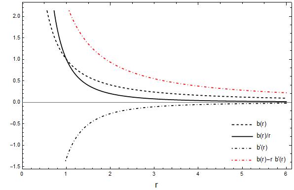
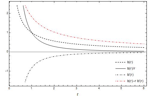
Figure 1: We show the behaviors of $b(r),b^{\prime}(r),b(r)/r$ and $b(r)-rb^{\prime}(r)$ versus $r$ in Eq.(33) for $\beta=-1.1$ and $r_{0}=1$ and $\omega=0.8$ (Left Panel) and $\omega=1$ (Right Panel).

matching with that found in Ref.Agrawal:2022atn . We recover the Ellis-Bronnikov (EB) shape function, $b(r)=\tfrac{r^{2}_{0}}{r}$, when $\omega=-\beta^{-1}$. We can show that the shape function (33) satisfies the usual properties displayed in Fig.(1). We can also simply check the expression of the flare-out condition given by

$$\frac{b(r)-rb^{\prime}(r)}{b(r)^{2}}=-\frac{2(\omega+1)\left(\frac{r}{r_{0}}\right)^{-\frac{2\beta\omega+\omega+3}{2\beta\omega-\omega+1}}}{(2\beta-1)r_{0}\omega+r_{0}}{\underset{r=r_{0}}{=}}-\frac{2(\omega+1)}{(2\beta-1)r_{0}\omega+r_{0}}>0\,.$$ (34)

which yields the constraints on $\omega$ and $\beta$:

$$\omega>0\land\beta<\frac{\omega-1}{2\omega}\,.$$ (35)

In this case, we can easily compute the energy density to obtain

$${\bar{\rho}}(r)=-\frac{1}{8\pi(\omega+1)r^{2}}\left(\frac{r}{r_{0}}\right)^{\frac{2(\omega+1)}{\omega(2\beta-1)+1}}\,.$$ (36)

which, on the throat becomes

$$\rho(r_{0})=-\frac{1}{8\pi(\omega+1)r_{0}^{2}}\,.$$ (37)

Using $\rho(r)$, we can compute $p_{r}$ and $p_{t}$ to obtain

$${\bar{p}}_{r} = -\frac{\omega}{8\pi(\omega+1)r^{2}}\left(\frac{r}{r_{0}}\right)^{\frac{2(\omega+1)}{\omega(2\beta-1)+1}}\,,$$ (38)

$${\bar{p}}_{t} = -\frac{\omega\beta}{8\pi(\omega+1)r^{2}}\left(\frac{r}{r_{0}}\right)^{\frac{2(\omega+1)}{\omega(2\beta-1)+1}}\,.$$ (39)

We see from Fig.(2) for constants $\omega$ & $\beta$, the NEC and SEC are violated at the wormhole throat $r=r_{0}$. In other words, we discover that at the wormhole throat $r=r_{0}$, we have for the energy condition $\rho^{\rm eff.}+p^{\rm eff.}_{r}<0$, along with the condition $\rho^{\rm eff.}+p^{\rm eff.}_{r}+2p^{\rm eff.}_{t}<0$, by arbitrary small values.

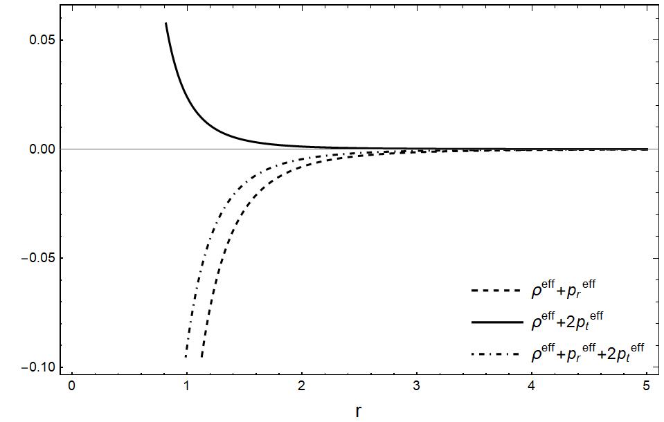
Figure 2: We show the behaviors of $\rho^{\text{eff}}+p_{r}^{\text{eff}}$, $\rho^{\text{eff}}+2p_{t}^{\text{eff}}$ and $\rho^{\text{eff}}+p_{r}^{\text{eff}}+2p_{t}^{\text{eff}}$ versus $r$ using $\beta=-1.1$, $r_{0}=1$ and $\omega=0.8$.

III.2 Variable $\omega$ & Constant $\beta$

In the preceding subsection, we have worked on the constant EoS and discussed some important properties of the shape function $b(r)$ illustrated in Fig.(1). However, variable EoS can also be considered. In case of $\omega=\omega(r)$, we come up with

$$\int\frac{1}{b(r)}\,db(r)=\int\frac{(2\beta\omega(r)+\omega(r)+3)}{r(2\beta\omega(r)-\omega(r)+1)}\,dr\,.$$ (40)

Therefore, we obtain

$$b(r)=r_{0}\,\exp\Big{(}\int\frac{(2\beta\omega(r)+\omega(r)+3)}{r(2\beta\omega(r)-\omega(r)+1)}\,dr\Big{)}\,.$$ (41)

with $r_{0}$ being a constant. Let us take a more general EoS:

$$\omega(r)=\frac{1}{\mu r}\,.$$ (42)

We find that

$$\omega(r){\underset{r=r_{0}}{\rightarrow}}\frac{1}{\mu r_{0}},\,\,\,\omega(r){\underset{\mu\rightarrow 0}{\rightarrow}}\infty\,,\quad{\rm and}\quad\omega(r){\underset{r\,{\rm or}\,\mu\rightarrow\infty}{\rightarrow}}0\,.$$ (43)

We solve Eq.(41) to obtain

$$b(r)=r_{0}\,\left(\frac{r}{r_{0}}\right)^{\frac{2\beta+1}{2\beta-1}}\left(\frac{1-2\beta-\mu r}{1-2\beta-\mu r_{0}}\right)^{\frac{4(\beta-1)}{2\beta-1}}\,.$$ (44)

We can also simply check the expression of the flare-out condition given by

$$\frac{b(r)-rb^{\prime}(r)}{b(r)^{2}}\Big{|}_{r=r_{0}}=\frac{2\mu r_{0}+2}{-\mu r_{0}^{2}-2\beta r_{0}+r_{0}}>0\,.$$ (45)

For more convenience, we take instead $\mu=\tfrac{\mu_{1}}{r_{0}}$ to have

$$\frac{b(r)-rb^{\prime}(r)}{b(r)^{2}}\Big{|}_{r=r_{0}}=\frac{2\mu_{1}+2}{-2\beta r_{0}-\mu_{1}r_{0}+r_{0}}>0\,.$$ (46)

With a flare-out condition, we find the constraints on $\beta$ and $\mu_{1}$:

$$\beta\leq 1\land-1<\mu_{1}<1-2\beta\land r_{0}>0\,.$$ (47)

If we take $\beta=-1.1$, we find that $-1<\mu_{1}<3.2$. However, in the following, we consider $\mu=-\tfrac{\beta}{r_{0}}$ and write

$$\omega(r)=-\frac{r_{0}}{\beta r}\,,$$ (48)

where

$$\omega(r){\underset{r=r_{0}}{\rightarrow}}-\frac{1}{\beta}\,,\quad{\rm and}\quad\omega(r){\underset{r\rightarrow\infty}{\rightarrow}}0\,.$$ (49)

In this case, $\beta$ is the only free parameter. Substituting Eq.(48) into Eq.(41), we find

$$b(r)=r_{0}\left(\frac{r}{r_{0}}\right)^{\frac{2\beta+1}{2\beta-1}}\left(\frac{\beta r-2\beta r_{0}+r_{0}}{r_{0}-\beta r_{0}}\right)^{\frac{4(\beta-1)}{2\beta-1}}\,.$$ (50)

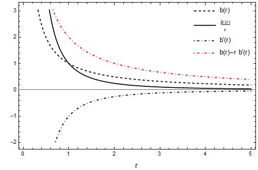
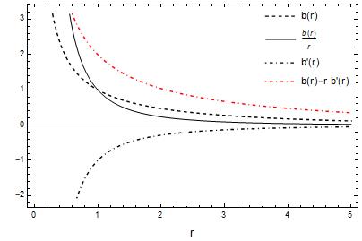
Figure 3: We show the behaviors of $b(r),b^{\prime}(r),b(r)/r$ and $b(r)-rb^{\prime}(r)$ versus $r$ in Eq.(50) for $r_{0}=1$ and $\beta=-0.01$ (Left Panel) and $\beta=-0.05$ (Right Panel).

We can quantify the features of a shape function $b(r)$. Assuming that $|\beta|\ll{\cal O}(1)$, we can expand $b(r)$ to the first order of $\beta$ to obtain

$$b(r)=\frac{r_{0}^{2}}{r}+\frac{4}{r}\left(-r_{0}^{2}\log\left(\frac{r}{r_{0}}\right)+rr_{0}-r_{0}^{2}\right)\beta+{\cal O}(\beta^{2})\,.$$ (51)

We see that when $|\beta|\ll{\cal O}(1)$ a shape function satisfies the usual properties as it should be. Notice that we can obtain the EB shape function, $b(r)=\tfrac{r^{2}_{0}}{r}$, when $\beta=0$. The behaviors of $b(r)$ can be seen in Fig.(3). In this case, we can easily compute the energy density to obtain

$${\bar{\rho}}(r)=-\frac{\beta}{4\pi(\beta-1)r^{2}}\left(\frac{r}{r_{0}}\right)^{\frac{2}{2\beta-1}+1}\left(\frac{\beta r-2\beta r_{0}+r_{0}}{r_{0}-\beta r_{0}}\right)^{\frac{2}{1-2\beta}+1}\,.$$ (52)

which, on the throat becomes

$${\bar{\rho}}(r_{0})=-\frac{\beta}{4\pi(\beta-1)r_{0}^{2}}\,.$$ (53)

Using ${\bar{\rho}}(r)$, we can compute ${\bar{p}}_{r}$ and ${\bar{p}}_{t}$ to obtain

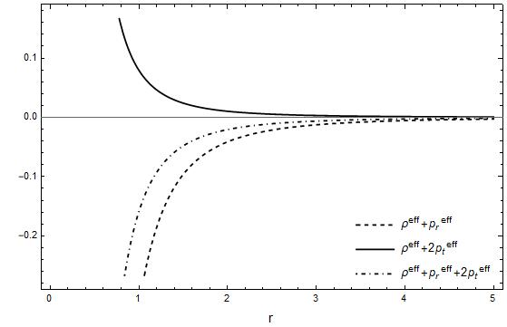
Figure 4: We show the behaviors of $\rho^{\text{eff}}+p_{r}^{\text{eff}}$, $\rho^{\text{eff}}+2p_{t}^{\text{eff}}$ and $\rho^{\text{eff}}+p_{r}^{\text{eff}}+2p_{t}^{\text{eff}}$ versus $r$ using $\beta=-0.01$, and $r_{0}=1$.

$${\bar{p}}_{r} = \frac{1}{4\pi(\beta-1)r^{2}}\left(\frac{r}{r_{0}}\right)^{\frac{2}{2\beta-1}}\left(\frac{\beta r-2\beta r_{0}+r_{0}}{r_{0}-\beta r_{0}}\right)^{\frac{2}{1-2\beta}+1}\,,$$ (54)

$${\bar{p}}_{t} = \frac{\beta}{4\pi(\beta-1)r^{2}}\left(\frac{r}{r_{0}}\right)^{\frac{2}{2\beta-1}}\left(\frac{\beta r-2\beta r_{0}+r_{0}}{r_{0}-\beta r_{0}}\right)^{\frac{2}{1-2\beta}+1}\,.$$ (55)

In this case, we also discover that the NEC & SEC are violated, i.e., $\rho^{\text{eff}}+p_{r}^{\text{eff}}<0,\,\rho^{\text{eff}}+p_{r}^{\text{eff}}+2p_{t}^{\text{eff}}<0$, by arbitrary small values, see Fig.(4).

IV Decoupled solutions

We consider the gravitational decoupling technique and consider two forms of the energy density for a smeared and particle-like gravitational source in the context of noncommutative geometry and a statically charged fluid.

IV.1 Non-commutative Geometry Density Profiles

In the context of noncommutative geometry, an interesting development of string/M-theory involves the requirement for quantizing spacetime. The non-commutativity of spacetime is encoded in the commutator $[{\bf x}^{\mu},{\bf x}^{\nu}]=i\theta_{\mu\nu}$, where $\theta_{\mu\nu}$ is an antisymmetric matrix which determines the fundamental discretization of spacetime. It has also been shown that noncommutativity flavors the smeared objects instead of the point-like structures in flat spacetime Smailagic:2003yb . Mathematically, the smearing permits substitution of the Dirac-delta function by a Gaussian distribution of minimal length $\sqrt{\theta}$.

Specifically, the formulation of the energy density for a gravitational source that is static, spherically symmetric, and resembles both a smeared and particle-like structure has been examined Nicolini:2005vd ; Lobo:2010uc given by

$$\rho_{\theta}(r)=\frac{M}{(4\pi\theta)^{3/2}}\exp\Big{(}-\frac{r^{2}}{4\theta}\Big{)}\,,$$ (56)

where the mass $M$ is diffused throughout a region of linear size $\sqrt{\theta}$ due to the intrinsic uncertainty encoded in the coordinate commutator. Like black holes, see e.g., Refs.Nicolini:2005vd ; DiGrezia:2007bxw , the wormhole metric is expected to be modified when a noncommutative spacetime is taken into account, see Rahaman:2014dpa ; Garattini:2008xz ; Rahman:2022pug . Moreover, we also get inspired by the work of Mehdipour when searching for a new fluid model. A Lorentzian distribution of particle-like gravitational source permits possible energy density profile as given in Ref.Mehdipour:2011mc ; Rahaman:2014dpa ; Liang:2012vx as follows:

$$\rho_{\phi}(r)=\frac{M\sqrt{\phi}}{\pi^{2}(r^{2}+\phi)^{2}}\,$$ (57)

with $\phi$ being the noncommutativity parameter. We next consider Eqs. (28)-(30) and employ the density profiles given above to quantify the decoupled solutions, $f(r)$. We assume that $\varepsilon^{0}_{0}=\rho_{\theta,\phi}$ and solve for $f(r)$ to obtain.

$$f(r)=\begin{cases}M\left(\text{erf}\left(\frac{r}{2\sqrt{\theta}}\right)-\text{erf}\left(\frac{r_{0}}{2\sqrt{\theta}}\right)-\frac{r}{\sqrt{\pi}\sqrt{\theta}}e^{-\frac{r^{2}}{4\theta}}+\frac{r_{0}}{\sqrt{\pi}\sqrt{\theta}}e^{-\frac{r_{0}^{2}}{4\theta}}\right)&\text{for}\,\rho_{\theta}=\varepsilon^{0}_{0}\,,\\ \frac{2M}{\pi}\left(\frac{r_{0}/\sqrt{\phi}}{\frac{r_{0}^{2}}{\phi}+1}-\frac{r/\sqrt{\phi}}{\frac{r^{2}}{\phi}+1}+\tan^{-1}\left(\frac{r}{\sqrt{\phi}}\right)-\tan^{-1}\left(\frac{r_{0}}{\sqrt{\phi}}\right)\right)&\text{for}\,\,\rho_{\phi}=\varepsilon^{0}_{0}\,.\end{cases}$$ (58)

We can simply check that a condition of $f(r=r_{0})=0$ is satisfied. Substituting $f(r)$ to Eq.(33), the original (traversable) wormhole solutions can be geometrically deformed. In this case, the original wormhole solution will be deformed by the above results. Therefore, we obtain for $\rho_{\theta}=\varepsilon^{0}_{0}$

$$\frac{b(r)}{\sqrt{\theta}} = \frac{r_{0}}{\sqrt{\theta}}\,\Big{(}\frac{r/\sqrt{\theta}}{r_{0}/\sqrt{\theta}}\Big{)}^{\frac{2\omega\beta+\omega+3}{2\omega\beta-\omega+1}}$$ (59)

$$+ \delta\frac{M}{\sqrt{\theta}}\left(\text{erf}\left(\frac{r}{2\sqrt{\theta}}\right)-\text{erf}\left(\frac{r_{0}}{2\sqrt{\theta}}\right)-\frac{r}{\sqrt{\pi}\sqrt{\theta}}e^{-\frac{r^{2}}{4\theta}}+\frac{r_{0}}{\sqrt{\pi}\sqrt{\theta}}e^{-\frac{r_{0}^{2}}{4\theta}}\right)\,,$$

and for $\rho_{\phi}=\varepsilon^{0}_{0}$

$$\frac{b(r)}{\sqrt{\phi}} = \frac{r_{0}}{\sqrt{\phi}}\,\Big{(}\frac{r/\sqrt{\phi}}{r_{0}/\sqrt{\phi}}\Big{)}^{\frac{2\omega\beta+\omega+3}{2\omega\beta-\omega+1}}$$ (60)

$$+ \frac{2\delta}{\pi}\frac{M}{\sqrt{\phi}}\left(\frac{r_{0}/\sqrt{\phi}}{\frac{r_{0}^{2}}{\phi}+1}-\frac{r/\sqrt{\phi}}{\frac{r^{2}}{\phi}+1}+\tan^{-1}\left(\frac{r}{\sqrt{\phi}}\right)-\tan^{-1}\left(\frac{r_{0}}{\sqrt{\phi}}\right)\right)\,.$$

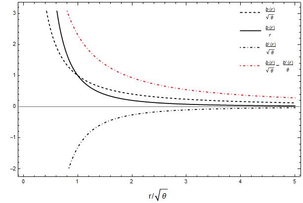
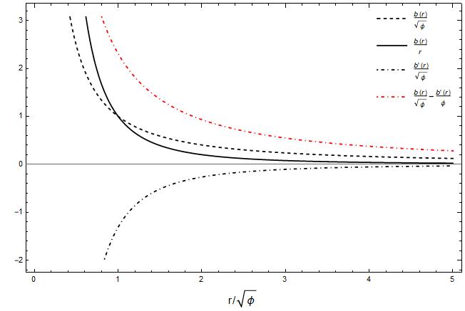
Figure 5: We show the behaviors of $\frac{b(r)}{\sqrt{\theta}},\frac{b^{\prime}(r)}{\sqrt{\theta}},\frac{b(r)}{\sqrt{\theta}}r$ and $\frac{b(r)-rb^{\prime}(r)}{\sqrt{\theta}}$ versus $\frac{r}{\sqrt{\theta}}$ in Eq.(59) for $\beta=-1.1$, $\omega=0.8$, $r_{0}=1$, $\delta=0.001$ and $\frac{M}{\sqrt{\theta}}=1$ (Left Panel) and $\frac{b(r)}{\sqrt{\phi}},\frac{b^{\prime}(r)}{\sqrt{\phi}},\frac{b(r)}{\sqrt{\phi}}r$ and $\frac{b(r)-rb^{\prime}(r)}{\sqrt{\phi}}$ versus $\frac{r}{\sqrt{\phi}}$ in Eq.(60) for $\beta=-1.1$, $\omega=0.8$, $r_{0}=1$, $\delta=0.001$ and $\frac{M}{\sqrt{\phi}}=1$ (Right Panel).

We can show that the shape function (59) and (60) satisfy the usual properties, see Fig.(5), namely the throat condition and so on. More specifically, using $b^{\prime}(r_{0})<1$, we have for Eq.(59):

$$\delta<\frac{1}{\frac{M}{\sqrt{\theta}}r_{0}^{2}}\Big{(}2\sqrt{\pi}me^{\frac{r_{0}^{2}}{4}}+2\sqrt{\pi}e^{\frac{r_{0}^{2}}{4}}\Big{)}\,,$$ (61)

and for Eq.(60):

$$\delta<\frac{e^{\frac{r_{0}^{2}}{4}}8\sqrt{\pi}}{\frac{M}{\sqrt{\phi}}r_{0}^{2}(mr_{0}-\beta+2)}\Big{(}mr_{0}+1\Big{)}\,,$$ (62)

where $m=\frac{2\omega\beta+\omega+3}{2\omega\beta-\omega+1}$.

IV.2 Electromagnetic field

The procedure used to obtain wormhole solutions can be extended to include also the electromagnetic field as an additional source. Here we include the contribution of an electric field generated by a point charge, $\cal{Q}$. The Einstein–Maxwell equations for a statically charged fluid can be given in terms of density $\rho(r)$, radial pressure $p_{r}$, and tangential pressure $p_{t}$. We follow the algebraic structure of stress-energy tensors for electromagnetic fields given in Dymnikova:2004zc ; Dymnikova:2021dqq by $T^{0}_{0}=T^{1}_{1}$ implying that $\rho=-p_{r}$. A pure spherically symmetric electromagnetic field without the contribution of any additional sources is determined by

$$T^{\rm EM}_{\mu\nu}=\frac{{\cal Q}^{2}}{8\pi r^{4}}{\rm diag.}(1,-1,1,1)\,,$$ (63)

which is conserved and traceless. We assume that $\varepsilon^{0}_{0}=T^{0}_{0}$ and solve for $f(r)$ to obtain.

$$f(r)=\frac{{\cal Q}^{2}}{2}\Big{(}\frac{1}{r_{0}}-\frac{1}{r}\Big{)}\,,$$ (64)

which a condition of $f(r=r_{0})=0$ is assumed. In this case, the original wormhole solution will be deformed by the above result. Therefore, we obtain

$$b(r)=r_{0}\,\Big{(}\frac{r}{r_{0}}\Big{)}^{\frac{2\omega\beta+\omega+3}{2\omega\beta-\omega+1}}+\delta\frac{{\cal Q}^{2}}{2}\Big{(}\frac{1}{r_{0}}-\frac{1}{r}\Big{)}\,.$$ (65)

We can show that the shape function (59) and (60) satisfy the usual properties, see Fig.(6), namely the throat condition and so on. We can also simply check the expression of the flare-out condition given by

$$\frac{b(r)-rb^{\prime}(r)}{b(r)^{2}}=\frac{2rr_{0}\left(\delta{\cal Q}^{2}((2\beta-1)\omega+1)(r-2r_{0})-4rr_{0}^{2}(\omega+1)\left(\frac{r}{r_{0}}\right)^{\frac{2\beta\omega+\omega+3}{2\beta\omega-\omega+1}}\right)}{((2\beta-1)\omega+1)\left(\delta{\cal Q}^{2}r-\delta{\cal Q}^{2}r_{0}+2rr_{0}^{2}\left(\frac{r}{r_{0}}\right)^{\frac{2\beta\omega+\omega+3}{2\beta\omega-\omega+1}}\right)^{2}}\,,$$ (66)

which yields the constraints at $r=r_{0}$:

$$\frac{\delta{\cal Q}^{2}(-2\beta\omega+\omega-1)-4r_{0}^{2}(\omega+1)}{2r_{0}^{3}((2\beta-1)\omega+1)}>0\quad{\longrightarrow}\quad{\cal Q}^{2}<\frac{-4r_{0}^{2}\omega-4r_{0}^{2}}{2\beta\delta\omega-\delta\omega+\delta}\,,$$ (67)

with the following conditions:

$$\delta>0\land\omega>0\land\left(r_{0}>0\land\beta<\frac{\omega-1}{2\omega}\right)\,.$$ (68)

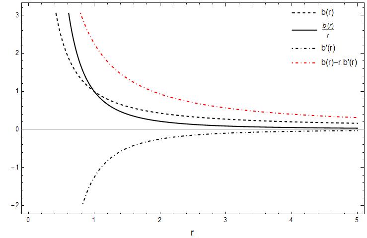
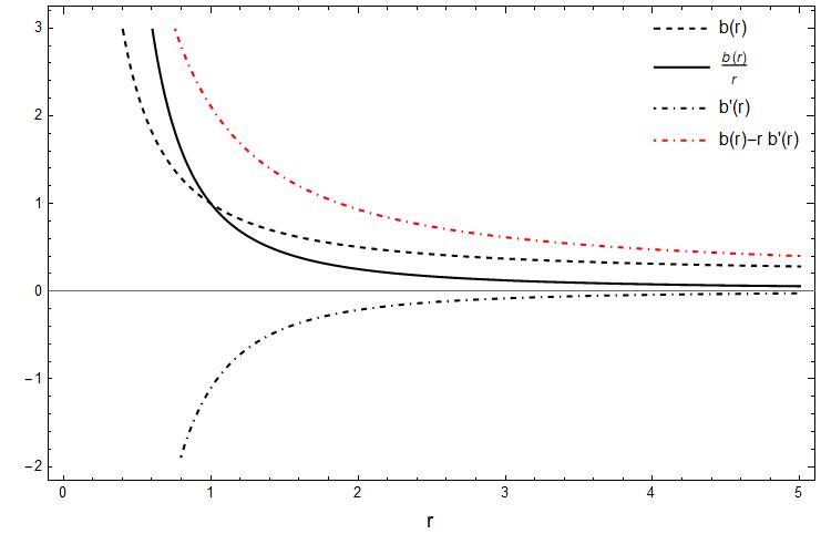
Figure 6: We show the behaviors of $b(r),b^{\prime}(r),b(r)/r$ and $b(r)-rb^{\prime}(r)$ versus $r$ in Eq.(69) for $\beta=-1.1$, $r_{0}=1$ and ${\cal Q}=1$ (Left Panel) and ${\cal Q}=2$ (Right Panel).

Moreover, in case of $\omega=\omega(r)$ and constant $\beta$, we have

$$b(r)=r_{0}\left(\frac{r}{r_{0}}\right)^{\frac{2\beta+1}{2\beta-1}}\left(\frac{\beta r-2\beta r_{0}+r_{0}}{r_{0}-\beta r_{0}}\right)^{\frac{4(\beta-1)}{2\beta-1}}+\delta\frac{{\cal Q}^{2}}{2}\Big{(}\frac{1}{r_{0}}-\frac{1}{r}\Big{)}\,.$$ (69)

We find for the flare-out condition to be satisfied:

$$\delta>0\land r_{0}>0\land|{\cal Q}|<2\sqrt{\frac{r_{0}^{2}}{\delta}}\,.$$ (70)

Notice that values of ${\cal Q}$ depend on a parameter $\delta$ and do not depend on $\beta$ in this case.

V Embedding diagram

In this section, we analyse the embedding diagrams to represent the wormhole solutions by considering an equatorial slice $\theta=\pi/2$ at some fix moment in time $t$ = constant. The metric then becomes

$$ds^{2}=\frac{1}{\left(1-\frac{b(r)}{r}\right)}dr^{2}+r^{2}d\phi^{2}\,,$$ (71)

Having embed the metric (71) into three-dimensional Euclidean space, we can visualize this slice. Here we parameterize spacetime using the cylindrical coordinates as

$$ds^{2}=dz^{2}+dr^{2}+r^{2}d\phi^{2}\,,$$ (72)

which can be rewritten as

$$ds^{2}=\Big{(}1+\Big{(}\frac{dz}{dr}\Big{)}^{2}\Big{)}dr^{2}+r^{2}d\phi^{2}\,.$$ (73)

Having compared Eq.(71) with Eq.(73), we come up with:

$$\frac{dz}{dr}=\pm\sqrt{\Big{(}\frac{r}{r-b(r)}-1\Big{)}}\,.$$ (74)

To test the results, we consider $b(r)$ given by Eq.(60) and Eq.(69). Invoking numerical techniques allows us to illustrate the wormhole shape given in Fig.(7). In Fig.(7), we consider various shape functions $b(r)$ given in Eq.(50), (60), and (69). We use $\beta=-1.1$ for all plots, and take $\delta=0.01,\,\omega=0.8$ and $M/\sqrt{\phi}=1$ for Eq.(60) and $\delta=0.01,\,\omega=0.8$ and ${\cal Q}=1$ for Eq.(69).

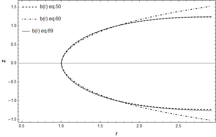
Figure 7: We display the embedding diagrams of various shape functions given in Eq.(50), (60), and (69).

VI Energy Conditions

We can further explore and check the energy conditions. In this section, we only consider the two types of energy conditions to examine the wormhole solutions. The first one is null energy condition (NEC) given as $T_{\mu\nu}k^{\mu}k^{\nu}\geq 0$, which determines the non-negative value of energy-momentum tensor with $k_{\mu}$ being null vectors. The NEC yields $\rho+p_{r}\geq 0$. Please note that the null energy condition (NEC) can be understood as the requirement for the energy of particles moving along a null geodesic, such as photons and massless particles, to remain non-negative. Additionally, the strong energy condition (SEC) defined as $\left(T_{\mu\nu}-\frac{1}{2}Tg_{\mu\nu}\right)X^{\mu}X^{\nu}\geq 0$ with $X_{\mu}$ being a timelike vector field, yields $\rho+2p_{t}\geq 0$ and $\rho+p_{r}+2p_{t}\geq 0$. However, the traversable wormholes in some particular models, e.g., Casimir wormholes Garattini:2019ivd ; Jusufi:2020rpw , need the (exotic) matter which violates the energy conditions.

VI.1 Constants $\omega$ & $\beta$

We first consider constants $\omega$ and $\beta$ and take $b(r)$ given in Eq.(59), and then compute the energy density. We find

$$\theta\,\rho(Y) = -\frac{1}{8\pi(\omega+1)Y^{2}}\left(\frac{Y}{Y_{0}}\right)^{\frac{2(\omega+1)}{\omega(2\beta-1)+1}}+\delta\frac{P}{(4\pi)^{3/2}}\exp\Big{(}-\frac{Y^{2}}{4}\Big{)}\,.$$ (75)

Using $\rho(Y)$, we can compute $p_{Y}$ and $p_{Y}$ to obtain

$$\theta\,p_{r}(Y) = -\frac{\omega}{8\pi(\omega+1)Y^{2}}\left(\frac{Y}{Y_{0}}\right)^{\frac{2(\omega+1)}{\omega(2\beta-1)+1}}$$ (76)

$$- \delta\frac{P}{8\pi^{3/2}Y^{3}}\Big{(}4\sqrt{\pi}\left(\text{erf}\left(\frac{Y_{0}}{2}\right)-\text{erf}\left(\frac{Y}{2}\right)\right)+\left(Y^{2}+4\right)Ye^{-\frac{Y^{2}}{4}}-4Y_{0}e^{-\frac{Y_{0}^{2}}{4}}\Big{)}\,,$$

$$\theta\,p_{t}(Y) = -\frac{\omega\beta}{8\pi(\omega+1)Y^{2}}\left(\frac{Y}{Y_{0}}\right)^{\frac{2(\omega+1)}{\omega(2\beta-1)+1}}$$ (77)

$$- \delta\frac{P}{4\pi\theta Y^{3}}\Big{(}\text{erf}\left(\frac{Y}{2}\right)-\text{erf}\left(\frac{Y_{0}}{2}\right)-\frac{e^{-\frac{Y^{2}}{4}}Y}{\sqrt{\pi}}+\frac{e^{-\frac{Y_{0}^{2}}{4}}\text{Y0}}{\sqrt{\pi}}\Big{)}\,,$$

where $Y\equiv r/\sqrt{\theta},\,P\equiv M/\sqrt{\theta}$. The stress-energy tensor (SET) can be computed using Eq.(11). We next consider constants $\omega$ and $\beta$ and take $b(r)$ given in Eq.(60), and then compute the energy density to obtain

$$\phi\,\rho(Z) = -\frac{1}{8\pi(\omega+1)Z^{2}}\left(\frac{Z}{Z_{0}}\right)^{\frac{2(\omega+1)}{\omega(2\beta-1)+1}}+\delta\frac{Q}{\pi^{2}}\left(\frac{1}{\left(1+Z^{2}\right)^{2}}\right)\,.$$ (78)

Using $\rho(Z)$, we can compute $p_{r}$ and $p_{t}$ to obtain

$$\phi\,p_{r}(Z) = -\frac{\omega}{8\pi(\omega+1)Z^{2}}\left(\frac{Z}{Z_{0}}\right)^{\frac{2(\omega+1)}{\omega(2\beta-1)+1}}$$ (79)

$$- \delta\frac{Q}{\pi^{2}Z^{3}}\left(-\frac{Z+3Z^{3}}{\left(1+Z^{2}\right)^{2}}+\frac{Z_{0}}{1+Z_{0}^{2}}+\text{tan}^{-1}(Z)-\text{tan}^{-1}(Z_{0})\right)\,,$$

$$\phi\,p_{t}(Z) = -\frac{\omega\beta}{8\pi(\omega+1)Z^{2}}\left(\frac{Z}{Z_{0}}\right)^{\frac{2(\omega+1)}{\omega(2\beta-1)+1}}$$ (80)

$$- \delta\frac{Q}{2\pi^{2}Z^{3}}\left(\frac{Z}{1+Z^{2}}-\frac{Z_{0}}{1+Z_{0}^{2}}-\text{tan}^{-1}(Z)+\text{tan}^{-1}(Z_{0})\right)\,,$$

where $Z\equiv r/\sqrt{\phi},\,Q\equiv M/\sqrt{\phi}$. We find from Fig.(6) that for small values of $\delta$ the NEC and SEC cannot be satisfied. However, since $b(r)$ is dependent on $\delta$, the usual properties of $b(r)$ cannot be satisfied, e.g., $b(r)/r\nrightarrow 0$ for $r\rightarrow\infty$ if $\delta$ is not so small, $\delta\gg{\cal O}(1)$.

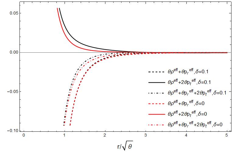
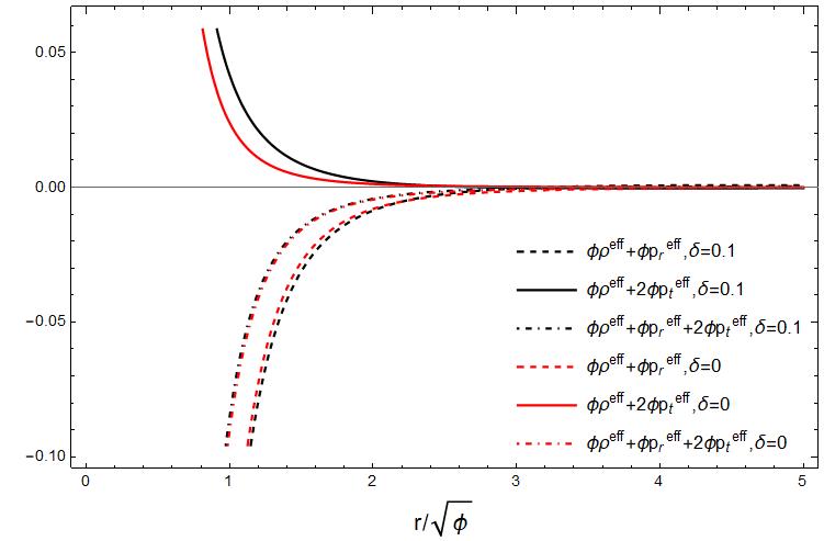
Figure 8: We show the behaviors of $\theta\rho^{\text{eff}}+\theta p_{r}^{\text{eff}}$, $\theta\rho^{\text{eff}}+2\theta p_{t}^{\text{eff}}$, $\theta\rho^{\text{eff}}+\theta p_{r}^{\text{eff}}+2\theta p_{t}^{\text{eff}}$ versus $r/\sqrt{\theta}$ using $\beta=-1.1$, $r_{0}=1$, $\omega=0.8$ for the Gaussian distribution Eq.(56) (Left panel), and $\phi\rho^{\text{eff}}+\phi p_{r}^{\text{eff}}$, $\phi\rho^{\text{eff}}+2\phi p_{t}^{\text{eff}}$, $\phi\rho^{\text{eff}}+\phi p_{r}^{\text{eff}}+2\phi p_{t}^{\text{eff}}$ versus $r/\sqrt{\phi}$ using $\beta=-1.1$, $r_{0}=1$, $\omega=0.8$ for the Lorentzian distribution Eq.(57) (Right panel).

We next consider constants $\omega$ and $\beta$ and take $b(r)$ given in Eq.(65), and then compute the energy density. We find

$$\rho(r) = -\frac{1}{8\pi(\omega+1)r^{2}}\left(\frac{r}{r_{0}}\right)^{\frac{2(\omega+1)}{\omega(2\beta-1)+1}}+\delta\frac{{\cal Q}^{2}}{8\pi r^{4}}\,.$$ (81)

Using $f(r)$, we can compute $p_{r}=\theta^{1}_{1}$ and $p_{t}=\theta^{2}_{2}$ to obtain

$$p_{r}(r) = -\frac{\omega}{8\pi(\omega+1)r^{2}}\left(\frac{r}{r_{0}}\right)^{\frac{2(\omega+1)}{\omega(2\beta-1)+1}}-\delta\frac{{\cal Q}^{2}}{8\pi r^{4}}\Big{(}\frac{2r}{r_{0}}-3\Big{)}\,,$$ (82)

$$p_{t}(r) = -\frac{\omega\beta}{8\pi(\omega+1)r^{2}}\left(\frac{r}{r_{0}}\right)^{\frac{2(\omega+1)}{\omega(2\beta-1)+1}}-\delta\frac{{\cal Q}^{2}}{8\pi r^{4}}\Big{(}1-\frac{r}{r_{0}}\Big{)}\,.$$ (83)

The behaviors of $\theta\rho^{\text{eff}}+\theta p_{r}^{\text{eff}}$, $\theta\rho^{\text{eff}}+2\theta p_{t}^{\text{eff}}$, $\theta\rho^{\text{eff}}+\theta p_{r}^{\text{eff}}+2\theta p_{t}^{\text{eff}}$ versus $r/\sqrt{\theta}$ for the Gaussian distribution Eq.(56), and $\phi\rho^{\text{eff}}+\phi p_{r}^{\text{eff}}$, $\phi\rho^{\text{eff}}+2\phi p_{t}^{\text{eff}}$, $\phi\rho^{\text{eff}}+\phi p_{r}^{\text{eff}}+2\phi p_{t}^{\text{eff}}$ versus $r/\sqrt{\phi}$ for the Lorentzian distribution Eq.(57) has been illustrated in Fig.(8). In Fig.(9), we notice that the NEC is also violated for the charged fluid deformation.

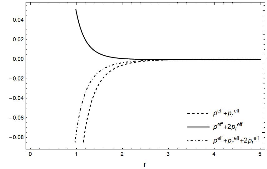
Figure 9: We show the behaviors of $\rho^{\text{eff}}+p_{r}^{\text{eff}}$, $\rho^{\text{eff}}+2p_{t}^{\text{eff}}$ and $\rho^{\text{eff}}+p_{r}^{\text{eff}}+2p_{t}^{\text{eff}}$ versus $r$ using $\beta=-1.1$, $r_{0}=1$ $\omega=0.8$ and ${\cal Q}=1$.

VI.2 Variable $\omega$ & Constant $\beta$

In this case, we can easily compute the energy density to obtain

$$\theta\,\rho(Y) = -\frac{\beta}{4\pi(\beta-1)Y^{2}}\left(\frac{Y}{Y_{0}}\right)^{\frac{2}{2\beta-1}+1}\left(\frac{\beta Y-2\beta Y_{0}+r_{0}}{Y_{0}-\beta Y_{0}}\right)^{\frac{2}{1-2\beta}+1}+\delta\frac{P}{(4\pi)^{3/2}}\exp\Big{(}-\frac{Y^{2}}{4}\Big{)}\,.$$ (84)

Using $\rho(Y)$, we can compute $p_{Y}$ and $p_{Y}$ to obtain

$$\theta\,p_{r}(Y) = \frac{1}{4\pi(\beta-1)Y^{2}}\left(\frac{Y}{Y_{0}}\right)^{\frac{2}{2\beta-1}}\left(\frac{\beta Y-2\beta Y_{0}+Y_{0}}{Y_{0}-\beta Y_{0}}\right)^{\frac{2}{1-2\beta}+1}$$ (85)

$$- \delta\frac{P}{8\pi^{3/2}Y^{3}}\Big{(}4\sqrt{\pi}\left(\text{erf}\left(\frac{Y_{0}}{2}\right)-\text{erf}\left(\frac{Y}{2}\right)\right)+\left(Y^{2}+4\right)Ye^{-\frac{Y^{2}}{4}}-4Y_{0}e^{-\frac{Y_{0}^{2}}{4}}\Big{)}\,,$$

$$\theta\,p_{t}(Y) = \frac{\beta}{4\pi(\beta-1)Y^{2}}\left(\frac{Y}{Y_{0}}\right)^{\frac{2}{2\beta-1}}\left(\frac{\beta Y-2\beta Y_{0}+Y_{0}}{Y_{0}-\beta Y_{0}}\right)^{\frac{2}{1-2\beta}+1}$$ (86)

$$- \delta\frac{P}{4\pi\theta Y^{3}}\Big{(}\text{erf}\left(\frac{Y}{2}\right)-\text{erf}\left(\frac{Y_{0}}{2}\right)-\frac{e^{-\frac{Y^{2}}{4}}Y}{\sqrt{\pi}}+\frac{e^{-\frac{Y_{0}^{2}}{4}}\text{Y0}}{\sqrt{\pi}}\Big{)}\,,$$

We next consider $\omega(r)$ and constant $\beta$ and take $b(r)$ given in Eq.(69), and then compute the energy density to obtain

$$\phi\,\rho(Z) = -\frac{\beta}{4\pi(\beta-1)Z^{2}}\left(\frac{Z}{Z_{0}}\right)^{\frac{2}{2\beta-1}+1}\left(\frac{\beta Z-2\beta Z_{0}+Z_{0}}{Z_{0}-\beta Z_{0}}\right)^{\frac{2}{1-2\beta}+1}+\delta\frac{Q}{\pi^{2}}\left(\frac{1}{\left(1+Z^{2}\right)^{2}}\right)\,.$$ (87)

Using $\rho(Z)$, we can compute $p_{r}$ and $p_{t}$ to obtain

$$\phi\,p_{r}(Z) = \frac{1}{4\pi(\beta-1)Z^{2}}\left(\frac{Z}{Z_{0}}\right)^{\frac{2}{2\beta-1}}\left(\frac{\beta Z-2\beta Z_{0}+Z_{0}}{Z_{0}-\beta Z_{0}}\right)^{\frac{2}{1-2\beta}+1}$$ (88)

$$- \delta\frac{Q}{\pi^{2}Z^{3}}\left(-\frac{Z+3Z^{3}}{\left(1+Z^{2}\right)^{2}}+\frac{Z_{0}}{1+Z_{0}^{2}}+\text{tan}^{-1}(Z)-\text{tan}^{-1}(Z_{0})\right)\,,$$

$$\phi\,p_{t}(Z) = \frac{\beta}{4\pi(\beta-1)Z^{2}}\left(\frac{Z}{Z_{0}}\right)^{\frac{2}{2\beta-1}}\left(\frac{\beta Z-2\beta Z_{0}+Z_{0}}{Z_{0}-\beta Z_{0}}\right)^{\frac{2}{1-2\beta}+1}$$ (89)

$$- \delta\frac{Q}{2\pi^{2}Z^{3}}\left(\frac{Z}{1+Z^{2}}-\frac{Z_{0}}{1+Z_{0}^{2}}-\text{tan}^{-1}(Z)+\text{tan}^{-1}(Z_{0})\right)\,.$$

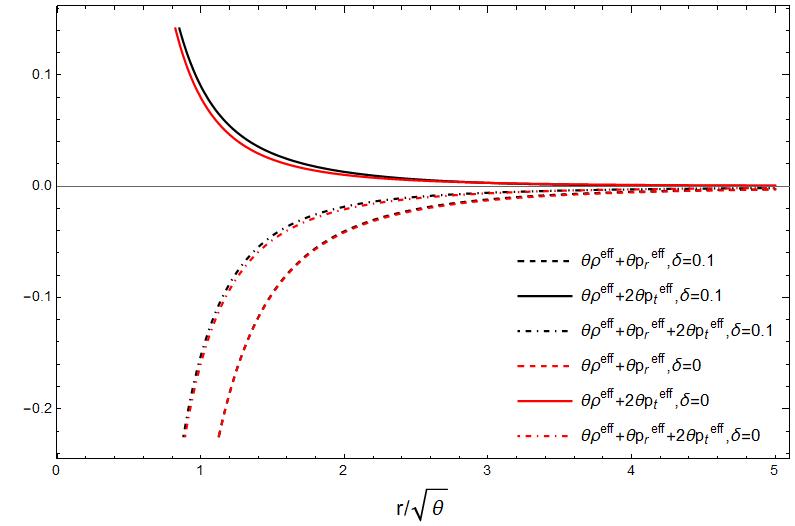
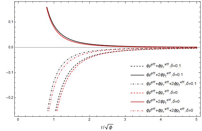
Figure 10: We show the behaviors of $\theta\rho^{\text{eff}}+\theta p_{r}^{\text{eff}}$, $\theta\rho^{\text{eff}}+2\theta p_{t}^{\text{eff}}$, $\theta\rho^{\text{eff}}+\theta p_{r}^{\text{eff}}+2\theta p_{t}^{\text{eff}}$ versus $r/\sqrt{\theta}$ using $\beta=-0.01$, $r_{0}=1$, $P=1$ for the Gaussian distribution Eq.(56) (Left panel), and $\phi\rho^{\text{eff}}+\phi p_{r}^{\text{eff}}$, $\phi\rho^{\text{eff}}+2\phi p_{t}^{\text{eff}}$, $\phi\rho^{\text{eff}}+\phi p_{r}^{\text{eff}}+2\phi p_{t}^{\text{eff}}$ versus $r/\sqrt{\phi}$ using $\beta=-0.01$, $r_{0}=1$, $Q=1$ for the Lorentzian distribution Eq.(57) (Right panel).

We consider $\omega(r)$ and constant $\beta$ and take $b(r)$ given in Eq.(69), and then compute the energy density. We find

$$\rho(r) = -\frac{\beta}{4\pi(\beta-1)r^{2}}\left(\frac{r}{r_{0}}\right)^{\frac{2}{2\beta-1}+1}\left(\frac{\beta r-2\beta r_{0}+r_{0}}{r_{0}-\beta r_{0}}\right)^{\frac{2}{1-2\beta}+1}+\delta\frac{{\cal Q}^{2}}{8\pi r^{4}}\,.$$ (90)

Using $f(r)$, we can compute $p_{r}=\theta^{1}_{1}$ and $p_{t}=\theta^{2}_{2}$ to obtain

$$p_{r}(r) = \frac{1}{4\pi(\beta-1)r^{2}}\left(\frac{r}{r_{0}}\right)^{\frac{2}{2\beta-1}}\left(\frac{\beta r-2\beta r_{0}+r_{0}}{r_{0}-\beta r_{0}}\right)^{\frac{2}{1-2\beta}+1}-\delta\frac{{\cal Q}^{2}}{8\pi r^{4}}\Big{(}\frac{2r}{r_{0}}-3\Big{)}\,,$$ (91)

$$p_{t}(r) = \frac{\beta}{4\pi(\beta-1)r^{2}}\left(\frac{r}{r_{0}}\right)^{\frac{2}{2\beta-1}}\left(\frac{\beta r-2\beta r_{0}+r_{0}}{r_{0}-\beta r_{0}}\right)^{\frac{2}{1-2\beta}+1}-\delta\frac{{\cal Q}^{2}}{8\pi r^{4}}\Big{(}1-\frac{r}{r_{0}}\Big{)}\,,$$ (92)

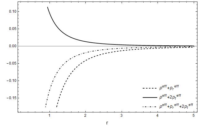
Figure 11: We show the behaviors of $\rho^{\text{eff}}+p_{r}^{\text{eff}}$, $\rho^{\text{eff}}+2p_{t}^{\text{eff}}$ and $\rho^{\text{eff}}+p_{r}^{\text{eff}}+2p_{t}^{\text{eff}}$ versus $r$ using $\beta=-0.01$, $r_{0}=1$ $\delta=0.01$and ${\cal Q}=1$.

The behaviors of $\theta\rho^{\text{eff}}+\theta p_{r}^{\text{eff}}$, $\theta\rho^{\text{eff}}+2\theta p_{t}^{\text{eff}}$, $\theta\rho^{\text{eff}}+\theta p_{r}^{\text{eff}}+2\theta p_{t}^{\text{eff}}$ versus $r/\sqrt{\theta}$ for the Gaussian distribution Eq.(56) and $\phi\rho^{\text{eff}}+\phi p_{r}^{\text{eff}}$, $\phi\rho^{\text{eff}}+2\phi p_{t}^{\text{eff}}$, $\phi\rho^{\text{eff}}+\phi p_{r}^{\text{eff}}+2\phi p_{t}^{\text{eff}}$ versus $r/\sqrt{\phi}$ for the Lorentzian distribution Eq.(57) can be seen in Fig.(10). In Fig.(11), we notice that the NEC is also violated for the charged fluid deformation.

VII Weak gravitational lensing

Embarking on this section, we revisit the Gauss-Bonnet theorem and embark on the calculation of the weak deflection angle for wormhole configurations. Our starting point is the expression for null geodesics, $ds^{2}=0$, which can be rearranged to yield:

$$dt^{2}=\gamma_{ij}dx^{i}dx^{j}=\frac{1}{W}dr^{2}+r^{2}d\Omega^{2},~{}$$ (93)

Within this context, indices i and j represent the spatial dimensions $(1to3)$, and $\gamma_{ij}$ denotes the optical metric. To utilize the Gauss-Bonnet theorem effectively, we must first calculate the Gaussian curvature associated with Eq.(50). This calculation is presented in detail here:

$$\mathcal{K}=\frac{R}{2} \approx \frac{6\beta^{2}r_{0}^{2}}{r^{4}}+\frac{2\beta r_{0}^{2}}{r^{4}}-\frac{r_{0}^{2}}{r^{4}}-\frac{6\beta^{2}r_{0}}{r^{3}}-\frac{2\beta r_{0}}{r^{3}}.~{}$$ (94)

Within this framework, $\gamma\equiv\det(\gamma_{ij})$ represents the determinant of the optical metric, and $R$ denotes the Ricci scalar. Let $D$ be a compact, oriented, nonsingular two-dimensional Riemannian surface characterized by its Euler characteristic $\chi(D)$and Gaussian curvature $\mathcal{K}$. This domain is enclosed by a piecewise-smooth curve with geodesic curvature $\kappa$. The link between the deflection angle of light and the Gaussian curvature stems from the Gauss-Bonnet theorem, which is invoked by employing the following expressions:

$$\int\int_{D}\mathcal{K}dS+\oint_{\partial D}\kappa dt+\sum_{i=1}\beta_{i}=2\pi\chi(D),~{}$$ (95)

Within this context, $dS$ represents the differential element of area, $\kappa$ denotes the geodesic curvature of the boundary, defined as $\kappa=|\nabla_{\dot{C}}\dot{C}|$ and $\beta_{i}$ represents the $i^{\text{th}}$ exterior angle. For a particular region $\tilde{D}$ enclosed by a geodesic $C_{1}$ extending from the source $S$ to the observer $O$ and a circular curve $C_{R}$ intersecting $C_{1}$ orthogonally at $S$ and $O$, Equation (95) reduces to:

$$\int\int_{\tilde{D}}\mathcal{K}dS+\int_{C_{R}}\kappa(C_{R})dt=\pi,~{}$$ (96)

During this derivation, we employed the conditions $\kappa(C_{1})=0$ and the Euler characteristic $\chi(\tilde{D})=1$. For the specific circular curve $C_{R}:=r(\phi)=R=\text{const}$, the non-zero segment of the geodesic curvature is calculated as:

$$\kappa(C_{R})=\left(\nabla_{\dot{C}_{R}}\dot{C}_{R}\right)^{r}=\dot{C}^{\phi}_{R}(\partial_{\phi}\dot{C}^{r}_{R})+\Gamma^{r}_{\phi\phi}(\dot{C}^{\phi}_{R})^{2},$$ (97)

In this context, $\dot{C}_{R}$ represents the directional derivative of the circular curve $C_{R}$, and $\Gamma^{r}_{\phi\phi}$ signifies the Christoffel symbol corresponding to the optical metric (93). As $R$ tends towards infinity, we arrive at:

$$\lim_{R\rightarrow\infty}\left[\kappa(C_{R})dt\right]=d\phi.~{}$$ (98)

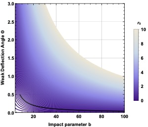
Figure 12: The deflection angle, $\Theta$, as expressed in Eq.(101) is plotted against the impact parameter $b$ using $\beta=-1.1$ in Eq.(50).

By substituting Eq. (98) into Eq. (96), we arrive at:

$$\int\int_{D}\mathcal{K}dS+\int_{0}^{\pi+\Theta}d\phi\pi=\pi.$$ (99)

In this context, the surface area on the equatorial plane is formulated as Gibbons:2008rj :

$$dS=\sqrt{\gamma}drd\phi$$ (100)

Following this, the weak deflection angle of light can be determined for Eq.50 as:

$$\Theta = -\int\int_{\tilde{D}}\mathcal{K}dS=-\int^{\pi}_{0}\int^{\infty}_{\frac{b}{\sin\phi}}\mathcal{K}dS$$ (101)

$$\simeq -\frac{3\pi\beta^{2}r_{0}^{2}}{2b^{2}}-\frac{\pi\beta r_{0}^{2}}{2b^{2}}+\frac{\pi r_{0}^{2}}{4b^{2}}+\frac{12\beta^{2}r_{0}}{b}+\frac{4\beta r_{0}}{b}.~{}$$

In this analysis, we utilized the zero-order particle trajectory $r=b/\sin\phi$, where $0\leq\phi\leq\pi$in the weak deflection limit. The dependence of the deflection angle on the impact parameter, as influenced by the wormhole geometry, is presented graphically in Fig.(12). Our findings reveal that the deflection angle is contingent upon the parameters $\beta$ and $r_{0}$ for $\omega(r)=-\tfrac{r_{0}}{\beta r}$. For specific values of $\beta$, it is observed that the deflection angle increases as $r_{0}$ grows. These results warrant comparison with those obtained using an alternative approach recently proposed in Ref.Li:2024ugi .

VIII Concluding Remarks

In this work, we investigate wormhole solutions invoking the Minimal Geometric Deformation (MGD) procedure within the framework of Unimodular Gravity. We employed a static and spherically symmetric Morris-Thorne traversable wormholes and considered both constants and variables in the equation of state parameter. More specifically, we considered $\omega={\rm cont.}$ and $\omega=\omega(r)=-\tfrac{r_{0}}{\beta r}$. We computed field equations and derived the shape functions. We showed that the usual properties of the obtained shape functions has been satisfied. We considered the gravitational decoupling technique and considered various forms of the energy density for a smeared and particle-like gravitational source in the context of noncommutative geometry and a statically charged fluid. We obtained the novel wormhole solutions showing the violation of the Null Energy Condition (NEC). We used the Gauss-Bonnet theorem to compute the weak deflection angle of light for the wormhole solutions. We also found that the deflection angle depends upon the parameter $\beta$ and $r_{0}$ for $\omega(r)=-\tfrac{r_{0}}{\beta r}$.

We can further test whether these wormholes be sustained by their own quantum fluctuations. In particular, the energy density of the graviton-one loop contribution to classical energy in a traversable wormhole background and the finite one loop energy density have to be considered as a self-consistent source for these wormhole geometries. To this end, we shall follow the existing publications, see e.g., Garattini:2005gd ; Garattini:2007ff ; Garattini:2008xz . However, the wormhole equation of state is still unknown and hence the present work can be tested by the wormhole observations, see. e.g., Abe:2010ap ; Toki:2011zu ; Godani:2021aub ; Ohgami:2015nra ; Dai:2019mse .

- (1) S. Weinberg, Rev. Mod. Phys. 61 (1989), 1-23
- (2) D. R. Finkelstein, A. A. Galiautdinov and J. E. Baugh, J. Math. Phys. 42 (2001), 340-346
- (3) M. Henneaux and C. Teitelboim, Phys. Lett. B 222 (1989), 195-199
- (4) W. G. Unruh, Phys. Rev. D 40 (1989), 1048
- (5) Y. J. Ng and H. van Dam, J. Math. Phys. 32 (1991), 1337-1340
- (6) E. Alvarez, JHEP 03 (2005), 002
- (7) G. F. R. Ellis, H. van Elst, J. Murugan and J. P. Uzan, Class. Quant. Grav. 28 (2011), 225007
- (8) G. F. R. Ellis, Gen. Rel. Grav. 46 (2014), 1619
- (9) C. Barceló, R. Carballo-Rubio and L. J. Garay, Phys. Rev. D 89 (2014) no.12, 124019
- (10) D. J. Burger, G. F. R. Ellis, J. Murugan and A. Weltman, [arXiv:1511.08517 [hep-th]].
- (11) E. Álvarez and S. González-Martín, Phys. Rev. D 92 (2015) no.2, 024036
- (12) M. Shaposhnikov and D. Zenhausern, Phys. Lett. B 671 (2009), 187-192
- (13) L. Smolin, Phys. Rev. D 84 (2011), 044047
- (14) P. Jain, A. Jaiswal, P. Karmakar, G. Kashyap and N. K. Singh, JCAP 11 (2012), 003
- (15) E. Alvarez and M. Herrero-Valea, Phys. Rev. D 87 (2013), 084054
- (16) A. Eichhorn, Class. Quant. Grav. 30 (2013), 115016
- (17) A. O. Barvinsky, N. Kolganov, A. Kurov and D. Nesterov, Phys. Rev. D 100 (2019) no.2, 0235425
- (18) A. O. Barvinsky and A. Y. Kamenshchik, Phys. Lett. B 774 (2017), 59-63
- (19) J. Ovalle, Phys. Rev. D 95 (2017) no.10, 104019
- (20) F. Tello-Ortiz, S. K. Maurya and P. Bargueño, Eur. Phys. J. C 81 (2021) no.5, 426
- (21) J. Ovalle, R. Casadio, R. da Rocha and A. Sotomayor, Eur. Phys. J. C 78 (2018) no.2, 122
- (22) R. Casadio and J. Ovalle, Gen. Rel. Grav. 46 (2014), 1669
- (23) R. Casadio, J. Ovalle and R. da Rocha, Class. Quant. Grav. 31 (2014), 045016
- (24) J. Ovalle and F. Linares, Phys. Rev. D 88 (2013) no.10, 104026
- (25) J. Ovalle, L. Á. Gergely and R. Casadio, Class. Quant. Grav. 32 (2015), 045015
- (26) R. Casadio, J. Ovalle and R. da Rocha, EPL 110 (2015) no.4, 40003
- (27) R. Casadio, J. Ovalle and R. da Rocha, Class. Quant. Grav. 32 (2015) no.21, 215020
- (28) J. Ovalle, Phys. Lett. B 788 (2019), 213-218
- (29) F. Tello-Ortiz, B. Mishra, A. Alvarez and K. N. Singh, Fortsch. Phys. 71 (2023) no.2-3, 2200108
- (30) G. W. Gibbons and M. C. Werner, Class. Quant. Grav. 25 (2008), 235009
- (31) M. C. Werner, Gen. Rel. Grav. 44, 3047-3057 (2012).
- (32) A. Ishihara, Y. Suzuki, T. Ono, T. Kitamura and H. Asada, Phys. Rev. D 94, no.8, 084015 (2016).
- (33) A. Ishihara, Y. Suzuki, T. Ono and H. Asada, Phys. Rev. D 95, no.4, 044017 (2017).
- (34) T. Ono, A. Ishihara and H. Asada, Phys. Rev. D 96, no.10, 104037 (2017).
- (35) G. Crisnejo and E. Gallo, Phys. Rev. D 97, no.12, 124016 (2018).
- (36) Z. Li and A. Övgün, Phys. Rev. D 101, no.2, 024040 (2020).
- (37) Z. Li, G. Zhang and A. Övgün, Phys. Rev. D 101, no.12, 124058 (2020).
- (38) K. Jusufi and A. Övgün, Phys. Rev. D 97, no.2, 024042 (2018).
- (39) A. Övgün, İ. Sakallı and J. Saavedra, JCAP 10, 041 (2018).
- (40) A. Övgün, Phys. Rev. D 98, no.4, 044033 (2018).
- (41) Y. Kumaran and A. Övgün, Turk. J. Phys. 45, no.5, 247-267 (2021) [arXiv:2111.02805 [gr-qc]].
- (42) W. Javed, M. Aqib and A. Övgün, Phys. Lett. B 829, 137114 (2022).
- (43) R. C. Pantig and A. Övgün, Eur. Phys. J. C 82, no.5, 391 (2022).
- (44) M. Okyay and A. Övgün, JCAP 01, no.01, 009 (2022).
- (45) A. Belhaj, M. Benali, A. El Balali, H. El Moumni and S. E. Ennadifi, Class. Quant. Grav. 37, no.21, 215004 (2020).
- (46) S. U. Islam, R. Kumar and S. G. Ghosh, JCAP 09, 030 (2020).
- (47) R. Kumar, S. G. Ghosh and A. Wang, Phys. Rev. D 101, no.10, 104001 (2020).
- (48) Q. Qi, Y. Meng, X. J. Wang and X. M. Kuang, Eur. Phys. J. C 83, no.11, 1043 (2023).
- (49) Y. Huang, Z. Cao and Z. Lu, JCAP 01, 013 (2024).
- (50) M. A. A. de Paula, H. C. D. Lima, Junior, P. V. P. Cunha and L. C. B. Crispino, Phys. Rev. D 108, no.8, 084029 (2023).
- (51) Y. Huang, B. Sun and Z. Cao, Phys. Rev. D 107, no.10, 104046 (2023).
- (52) Y. Huang and Z. Cao, Phys. Rev. D 106, no.10, 104043 (2022).
- (53) N. Parbin, D. J. Gogoi, J. Bora and U. D. Goswami, Phys. Dark Univ. 42, 101315 (2023).
- (54) M. Halla and V. Perlick, Phys. Rev. D 107, no.2, 024048 (2023)
- (55) M. Cadoni, A. P. Sanna and M. Tuveri, Phys. Rev. D 102 (2020) no.2, 023514
- (56) A. S. Agrawal, B. Mishra and P. H. R. S. Moraes, Eur. Phys. J. Plus 138 (2023) no.3, 275
- (57) B. J. Carr, T. Harada and H. Maeda, Class. Quant. Grav. 27 (2010), 183101
- (58) S. Bahamonde, M. Jamil, P. Pavlovic and M. Sossich, Phys. Rev. D 94 (2016) no.4, 044041
- (59) P. E. Kashargin and S. V. Sushkov, Universe 6 (2020) no.10, 186
- (60) D. Wang and X. h. Meng, Eur. Phys. J. C 76 (2016) no.9, 484
- (61) M. Cataldo and P. Meza, Phys. Rev. D 87 (2013) no.6, 064012
- (62) R. Garattini and P. Channuie, [arXiv:2311.04620 [gr-qc]].
- (63) A. Smailagic and E. Spallucci, J. Phys. A 36 (2003), L467
- (64) P. Nicolini, A. Smailagic and E. Spallucci, Phys. Lett. B 632 (2006), 547-551
- (65) F. S. N. Lobo and R. Garattini, JHEP 12 (2013), 065
- (66) E. Di Grezia, G. Esposito and G. Miele, J. Phys. A 41 (2008), 164063
- (67) R. Garattini and F. S. N. Lobo, Phys. Lett. B 671 (2009), 146-152
- (68) F. Rahaman, I. Karar, S. Karmakar and S. Ray, Phys. Lett. B 746 (2015), 73-78
- (69) N. Rahman, M. Kalam, A. Das, S. Islam, F. Rahaman and M. Murshid, Eur. Phys. J. Plus 138 (2023) no.2, 146
- (70) S. H. Mehdipour, Eur. Phys. J. Plus 127 (2012), 80
- (71) J. Liang and B. Liu, EPL 100 (2012) no.3, 30001
- (72) I. Dymnikova, Class. Quant. Grav. 21 (2004), 4417-4429
- (73) I. Dymnikova and E. Galaktionov, J. Phys. Conf. Ser. 2103 (2021) no.1, 012078
- (74) R. Garattini, Eur. Phys. J. C 79 (2019) no.11, 951
- (75) K. Jusufi, P. Channuie and M. Jamil, Eur. Phys. J. C 80 (2020) no.2, 127
- (76) Z. Li, [arXiv:2401.12525 [gr-qc]].
- (77) R. Garattini, Class. Quant. Grav. 22 (2005), 1105-1118
- (78) R. Garattini and F. S. N. Lobo, Class. Quant. Grav. 24 (2007), 2401-2413
- (79) F. Abe, Astrophys. J. 725 (2010), 787-793
- (80) Y. Toki, T. Kitamura, H. Asada and F. Abe, Astrophys. J. 740 (2011), 121
- (81) N. Godani and G. C. Samanta, Annals Phys. 429 (2021), 168460
- (82) T. Ohgami and N. Sakai, Phys. Rev. D 91 (2015) no.12, 124020
- (83) D. C. Dai and D. Stojkovic, Phys. Rev. D 100 (2019) no.8, 083513