Simulation of the formation of patterned polymer films:
using composite substrates in evaporative lithography
Abstract
The continuing development of evaporative lithography is important for many areas such as the creation of photonic crystals for optronics and microelectronics, the development of biosensors for medical applications and biotechnology, and for the formation of functional coatings for nanotechnology, including the application of thin, protective polymer coatings. The article proposes a mathematical model that allows us to explain the basic mechanisms of the formation of thin polymer films (less than 50 m thick) during their deposition onto a composite substrate by methanol evaporation from a solution. If the thermal conductivity of the substrate is spatially non-uniform, this results in inhomogeneous evaporation along the free film surface. Therefore, as the film dries, a patterned polymer coating is left behind on the substrate. The mathematical model described here is based on the lubrication approximation and takes into account the dependence of the solution density on the concentration. The numerical computation results are in qualitative agreement with the experimental data of other authors. The article shows that solutal Marangoni flow plays a primary role in the process under consideration. This study allows us to better understand the mechanisms that can be used in evaporative lithography.
I Introduction
The evaporative self-assembly process allows different patterns of deposition to be obtained on a substrate as the droplets and films dry Deegan et al. (1997); Deegan (2000); Sefiane (2014). A further logical progression of this method is evaporative lithography Routh and Russel (1998); Harris et al. (2007); Harris and Lewis (2008). Various key parameters can be altered to influence the evaporation to produce particular deposit patterns. These approaches can be classified as passive or active methods. In passive methods the parameters are configured ahead of starting process. Active methods are controlled by parameters that can be adjusted in real time. A separate subgroup, of “hybrid methods”, can be considered, where evaporative lithography is combined with other methods related, or not, to evaporative self-assembly. A large number of examples are described in the review Kolegov and Barash (2020). Here we will mention only a few articles in this field, including some relatively recent ones.
When solving problems in the field of evaporative lithography, numerical methods are often used to cope with the nonlinearity of the differential equations, the need to consider several subdomains (liquid, substrate and air) and the complex geometry of the computational domain. However, for some special cases, an analytical solution to the problem may be obtained, for example, the case of an axisymmetric colloidal drop drying on a horizontal impermeable substrate, if we consider the stationary vapor flux density with a spatial heterogeneity described by an empirical expression using an adjustable parameter D'Ambrosio et al. (2023). This model allows one to calculate the field of the capillary flow affecting the transfer of colloidal particles that depends on the character of the evaporation (for example, can increase either near the drop periphery or in center, while in other cases evaporation occurs uniformly over the entire free surface). An analytical solution can also be obtained for the Marangoni flow Li, Kar, and Kumar (2019). For example, such a flow can be controlled by non-uniform heating of the substrate (cell) Al-Muzaiqer et al. (2021a, b). There is also another example: when a temperature gradient arises in a drop of water with suspended gold nanoparticles under local illumination of the free surface. This results in a surface tension gradient and, as a consequence, thermal Marangoni flow develops. Such subregion heating occurs if the light wavelength matches the plasmonic absorption of the gold nanoparticles Farzeena and Varanakkottu (2022). This allows one to control the process of deposit formation in real time and therefore to obtain different patterns, including of particle mixtures (gold nanoparticles and polymer microspheres) on the substrate. The local irradiation time affects the morphology of such deposits. In addition, the deposit morphology is often affected by the substrate wettability Perkins-Howard et al. (2022). A special chemical surface treatment may be used to make a hydrophobic substrate hydrophilic in order to obtain densely packed microspheres instead of disordered structures. This difference is the result of the capillary attraction of particles that occurs on a hydrophilic surface in a thin liquid film. Evaporative self-assembly can also enable microsphere masks to be obtained on a solid surface for further use in colloidal lithography Perkins-Howard et al. (2022). In the case of bioliquid droplets, the deposit formation may be controlled using solutal Marangoni flow Hegde et al. (2022). When an ethanol drop hanging on the tip of a syringe needle is placed above a sessile drop of bioliquid (above its free surface in a particular, local subregion), a surface tension gradient appears. This results from ethanol vapor being adsorbed at the “liquid–air” interface, thereby reducing the bioliquid’s surface tension. This method can be used in biomedical applications. The coffee ring effect can be suppressed by directing an infrared laser beam onto the top of a sessile drop of saline solution, resulting in the formation of a central crystalline deposit Li et al. (2021). The local liquid heating results in a temperature gradient on the free surface and, therefore, in spatially inhomogeneous evaporation. This approach can produce a spot-like deposit formation Li et al. (2021). An experiment Goy et al. (2022) was performed to measure the resulting spot size versus the power of the IR laser and the diameter of the light beam directed at the top of the sessile water drop. The central spot was surrounded by a ring formed at the contact line. Based on analytical flow velocity estimates, the authors showed that this form of deposit is associated with the competition between the capillary and Marangoni flows Goy et al. (2022) (stagnation point where is the radius of the base of the drop). Another way to achieve the deposition of particles in specific locations is to use a substrate with an array of micropores Berneman et al. (2021). If a reduced atmospheric pressure, close to a vacuum, is created under the substrate, the liquid quickly evaporates from the sessile drop through the substrate micropores. A flow of liquid occurs carrying particles towards the pores. To prevent the particles from being sucked into the vacuum region along with the liquid molecules, they must have a size exceeding the pore diameter Berneman et al. (2021). Evaporative lithography allows the deposition of functional coatings. For example, electrically conductive ink can be deposited into microchannels of a topographically structured surface through nanoparticle transfer by the capillary flow induced by evaporation Corletto and Shapter (2021). Thermocapillary flow in a liquid film can be affected by spatial inhomogeneity of the substrate’s thermal conductivity. The lubrication approximation together with analytical solution have been used to study the influence of a series of parameters on the flow of clear liquid and the shape of the free film’s surface on a composite substrate Gambaryan-Roisman (2010). A continuation of that work investigated non-stationary heat distribution in a solid substrate Gambaryan-Roisman (2012). The influence of non-uniform thermal properties and non-uniform substrate heating on thermocapillary flow and on free film surface deformation is described in detail in the review Gambaryan-Roisman (2015). Variable-stiffness composite substrates allow control of the deposit geometry. For example, if such a substrate includes two surface subregions where the outer one is hard and the inner one is soft, then a stripe of deposited particles is formed at the boundary of these subregions Iqbal et al. (2022). In this way, stripes may be obtained not only along the perimeters of circles (coffee ring effect) but also along those of squares, triangles, etc. The overall duration of evaporation from a liquid droplet depends on the substrate’s thermal conductivity. This parameter can be adjusted in a graphene-polydimethylsiloxane substrate, for example. The higher the graphene concentration in the composite substrate the higher its thermal conductivity, causing the sessile drop to evaporate faster Goel et al. (2019). Chemically heterogeneous substrates with uneven distribution of surface wettability (from hydrophilic to hydrophobic) result in instability of liquid nanofilms, up to the appearance of local ruptures. This process can be described using the stochastic lubrication equation and the molecular dynamics method Zhao, Zhang, and Si (2023).
The purpose of this article is to study, numerically, the formation of a patterned polymer coating associated with a film drying on a particular composite substrate that had previously been experimentally observed Cavadini et al. (2013). Several mechanisms that may presumably influence this process are discussed here. A direct comparison of the numerical results and experimental data Cavadini et al. (2013) is then used to determine the mechanism playing the primary role.
II Methods
II.1 Physical problem statement
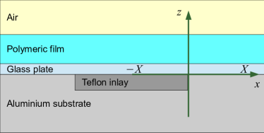
Take a liquid polymer film (methanol-poly(vinyl acetate) solution with 67 wt.% methanol) being applied to a thin glass plate located on top of an aluminum substrate. A thin Teflon inlay is embedded into the aluminum substrate (Fig. 1). The film height corresponds to the finite size but its length and width are assumed infinite (the author and readers can imagine this mentally for the convenience of the mathematical description, although in the actual experiment all dimensions were finite). We also assume that the Teflon inlay has a finite width and infinite length. In addition, the height of the Teflon layer is much less than the substrate height so we can assume a zero thickness coating. In consideration of the foregoing, let us consider the problem in a one-dimensional formulation where the film thickness (height) depends on the coordinate and time . Here, the axis is disregarded since the film thickness along it will be uniform throughout the process. Heat exchange between the liquid and substrate occurs through the interface between these two phases. It is important to keep in mind that this heat exchange is spatially inhomogeneous, depending on whether the substance in contact with the film is Teflon or aluminum. For this reason, we take into account the substrate thermal conductivity dependence only along the coordinate. We assume that the glass plate thickness is much less than that of the aluminum substrate, . Thus, the thermal properties of the plate do not need to be considered here. The values and were not specified in the experiment Cavadini et al. (2013). The substrate thickness has been determined approximately based on Fig. 3 of the Ref. Cavadini et al. (2013) ( 2 mm). The initial thickness of the polymer film is known, 150 m. The substrate is located perpendicular to the gravity vector. Point corresponds to the center of the Teflon strip so we consider this to be the boundary of symmetry. The opposite point corresponds to the boundary located at a sufficient distance from the point , coinciding with the edge of the Teflon inlay. Let us estimate the time of thermal, , and diffusional relaxation, , along the vertical direction of the liquid layer, 0.2 s and 24.7 s. Note that , where is the evaporation time. Therefore, we disregard the mass and heat transfer along the vertical direction.
The physical and geometric parameters of the problem are presented in Table 1. The values of most of the physical quantities are taken from various handbooks. See Appendix A for more details on the parameters: , , , , and .
| Symbol | Parameter | Value | UoM |
|---|---|---|---|
| Gravity acceleration | 9.8 | m/s2 | |
| Volumetric thermal expansion factor of methanol | K-1 | ||
| Volumetric thermal expansion factor of air | K-1 | ||
| Heat of evaporation | J/kg | ||
| Specific heat capacity of the liquid | 2619 | J/(kg K) | |
| Specific heat capacity of aluminum substrate | 903 | J/(kg K) | |
| Specific heat capacity of dry air | 1007 | J/(kg K) | |
| Surface tension coefficient of methanol Cavadini et al. (2013) | N/m | ||
| Dynamic viscosity of methanol | s Pa | ||
| Methanol density | 792 | kg/m3 | |
| Air density | 1.225 | kg/m3 | |
| Kinematic viscosity of methanol | m2/s | ||
| Kinematic viscosity of air | m2/s | ||
| Aluminum density | kg/m3 | ||
| Thermal conductivity coefficient of the liquid | 0.2 | W/(m K) | |
| Thermal conductivity coefficient of aluminum | 236 | W/(m K) | |
| Thermal conductivity coefficient of Teflon | 0.25 | W/(m K) | |
| Thermal conductivity coefficient of air | 0.026 | W/(m K) | |
| Thermal diffusion coefficient of the liquid | m2/s | ||
| Thermal diffusion coefficient of air | m2/s | ||
| “Sol–gel” phase transition concentration | 0.58 | – | |
| Initial solution concentration Cavadini et al. (2013) | 0.33 | – | |
| Saturation temperature | 338 | K | |
| Ambient temperature Cavadini et al. (2013) | 303 | K | |
| Temperature difference between substrate and the liquid | 2.36 (Table 1 Ahlers and Xu (2001)) | K | |
| Temperature difference between the substrate and air | 10 (Fig. 11 Cavadini et al. (2013)) | K | |
| “Liquid–substrate” convective heat exchange coefficient | 61 | W/(m2K) | |
| “Liquid–air” convective heat exchange coefficient | 50 (see Appendix A) | W/(m2K) | |
| “Substrate–air” convective heat exchange coefficient | 0.033 | W/(m2K) | |
| Mutual diffusion coefficient for concentration Tönsmann, Scharfer, and Schabel (2021) | m2/s | ||
| Evaporation process time | 60 | s | |
| Molar weight of the liquid | 0.032 | kg/mol | |
| Universal gas constant | 8.31 | J/(mol K) | |
| Polymer density | 1190 | kg/m3 | |
| Density difference between the polymer and liquid | 398 | kg/m3 | |
| Temperature gradient of surface tension | N/(m K) | ||
| Horizontal region size | 1 | cm | |
| Film thickness (height) Cavadini et al. (2013) | 150 | m | |
| Substrate thickness (height) | 2 | mm |
As the alcohol evaporates, the film surface cools. A vertical temperature gradient appears in the system. Due to the temperature difference, the substrate loses its heat to the film through thermal conductivity. But, as mentioned earlier, heat transfer will occur non-uniformly along the “liquid–substrate” interface, because the substrate is a composite (aluminum conducts heat better than Teflon). The result is that a horizontal temperature gradient appears, promoting non-uniform liquid evaporation along the free film surface. This, in turn, results in the appearance of capillary flows associated with a Laplace pressure gradient. Such a flow is sometimes called compensatory flow since the root cause is non-uniform evaporation, resulting in a curvature change of the free film surface. We neglect the influence of gravity on the fluid flow since a thin liquid film is being considered with a capillary length of 2.4 mm (). Another potential mass transfer mechanism involves thermocapillary flow. Indeed, the temperature gradient along the free surface results in a surface tension difference and, consequently, this leads to the thermal Marangoni effect. The thermocapillary flow is directed along the free surface from the low to the high surface tension regions, and therefore from the warm region to the relatively cold one. Moreover, the vapor flux density gradient affects the admixture concentration difference along the free liquid surface, also affecting the non-uniform change in surface tension, and, consequently, the appearance of solutal Marangoni flow. Convective and diffusive mass and heat transfer can enhance or weaken the above effects generally, affecting the formation of the solid, patterned polymer coating.
In the experiment Cavadini et al. (2013), an air stream was passed over the film with different velocity values, 0.5, 1, and 1.5 m/s. The results showed that the profile of the dried polymer film only weakly depended on in the considered range of values. In this regard, the air flow is not taken into account here.
II.2 Mathematical model
The horizontal mass and heat transfer (along the axis) are important in the system under consideration since diffusion processes smooth out the differences along the vertical direction ( axis), and uniform distribution is expected along the axis. Let us describe the problem in a one-dimensional formulation. It is convenient to write the mathematical model in dimensionless form to reduce the number of problem parameters (see Table 2). The lubrication approximation may be used to describe the hydrodynamics for a thin film ( 150 m). The liquid is assumed incompressible. In this case, the expression for the horizontal flow velocity averaged over the liquid layer height is written as Al-Muzaiqer et al. (2021b)
| (1) |
where , , , , and are the functions depending on the coordinate and time . Here, is the polymer mass fraction (concentration) in the solution, is the viscosity, and is the surface tension (for information on and see section II.3). The tilde symbol denotes dimensionless quantities. To convert to dimensional quantities, the following relations should be used: , , , , , and . Here, we use the characteristic length 1 mm, velocity 1 mm/s, and time 1 s. In (1), the Heaviside function is added to eliminate the mass transfer by convective flow in the model when the critical concentration is reached. Formula (1) takes into account both capillary flow and Marangoni flow.
| Symbol | Parameter | Value |
|---|---|---|
| Capillary number | ||
| Fourier number (liquid) | 0.1 | |
| Fourier number (substrate) | 0.08 | |
| Bulygin number | 1.5 | |
| Grashof number (liquid) | 70 | |
| Grashof number (air) | 1.5 | |
| Prandtl number (liquid) | 6.7 | |
| Prandtl number (air) | 0.7 | |
| Rayleigh number (liquid) | 469 | |
| Rayleigh number (air) | 1.05 | |
| Nusselt number (liquid)111Parameters and are described in Appendix A. | 0.3 | |
| Nusselt number (air) | ||
| Modified Graetz number (liquid to substrate heat transfer) | 34 | |
| Modified Graetz number (substrate to liquid heat transfer) | 40 | |
| Modified Graetz number (liquid to air heat transfer) | 41.5 | |
| Modified Graetz number (substrate to air heat transfer) | 37.8 | |
| Peclet number | 1099 |
On the other hand, when deriving equations based on the conservation law for the polymer and solution as a whole, we consider the concentration dependence of the liquid density. For more information on the concepts of quasi-incompressible and semi-compressible fluids, see Ref. Roubíček (2021). In this case, the spatiotemporal film thickness evolution is described by the equation
| (2) |
where the vapor flux density and solution density are expressed by the empirical formulas in section II.3.
The polymer concentration in solution is described by the convection-diffusion equation
| (3) |
where is the Peclet number (Table 2) and is the mutual diffusion coefficient (section II.3). In Eq. (3), the Heaviside function allows us to “turn off” diffusion when a critical concentration is reached. The derivation of the equations (2) and (3) is presented in Appendix B.
Heat transfer in a liquid is described by the equation Kolegov (2018)
| (4) |
where is the liquid temperature (, where is the characteristic temperature), is the thermal conductivity coefficient of the substrate (), is the Fourier number for the liquid, is the Bulygin number, and and are the modified Graetz numbers (see Table 2 and section II.3). Eq. (4) takes into account convective and diffusive heat transfers (thermal conductivity), evaporative cooling, and heat exchange via the “liquid–substrate” and “liquid–air” boundaries. Previously, Eq. 4 was obtained by considering the thermal energy balance in an elementary liquid column under the assumption of constant density Kolegov (2018).
Let us write a separate equation for the substrate temperature Al-Muzaiqer et al. (2021b)
| (5) |
where is the substrate temperature (), is the Fourier number for the substrate, and and are the modified Graetz numbers (see Table 2). Eq. (5) takes into account both the substrate thermal conductivity and the heat exchange with the liquid and the environment. The mathematical model is a system of partial differential equations (1)–(5).
II.3 Closing relations
The mathematical model described in section II.2 can be supplemented with closing relations for the functions , , , , and . To accomplish this, we will use empirical formulas.
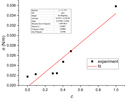
The surface tension depends on the solution temperature and concentration. As a first approximation, we will use a linear dependence (Fig. 2). The values of the parameters and are chosen to approximate the experimental data Cavadini et al. (2015) (, ). This dependence allows us to take into account both the solutal Marangoni flow and the thermal one in formula (1). In order to eliminate the solutal Marangoni flow from the model, it is sufficient to use the value . The thermal Marangoni flow may be eliminated from consideration via . Capillary flow may be eliminated from the model by multiplying the first term in parentheses in formula (1) by a small number (for example, 10-9).
The methanol density varies within 1% in the considered temperature range, therefore, we take into account only the concentration dependence, , where . Thus, we also use a linear dependence for density as a first-order approximation.
To describe the dependence of the vapor flux density on liquid temperature, we use the Hertz–Knudsen formula
with an additional factor added in order to simulate at in the model (evaporation stops when the liquid runs out). It is difficult to find experimental data on the vapor flux density versus concentration of the solution considered here, but they would be very useful in order to develop a more accurate model. The empirical parameter determines the liquid evaporation rate. The value is adjusted so that the time of complete liquid evaporation approximately corresponds to the experimental time Cavadini et al. (2013). The characteristic vapor flux density is taken to be 0.8 kg/(m2s). We assume that the concentration of methanol vapor away from the film is close to zero, therefore, the partial pressure is Sazhin (2006). The saturated vapor pressure depends on temperature. This dependence can be described using the semi-empirical Antoine equation,
where the constants 133.3 and 273.15 are used to convert from one unit of measurement to another (from mm Hg to Pa and from ∘C to K). The following empirical parameter values are used for methanol: 8.08097, 1582.27, and 239.7.
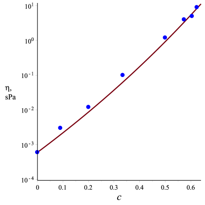
The methanol viscosity varies within 6% in the considered temperature range, which is very insignificant. Therefore, we will only take into account the dependence of viscosity on solution concentration. To accomplish this, we use the Mooney formula
where and . The empirical parameters and are determined using the least squares method (Fig. 3). The exponent will return huge values at high concentrations so we can multiply its argument by the Heaviside function,
to minimize computational problems. The fact is that, at , the viscosity . Due to the Heaviside function, the expression for the flow velocity (1) gives the value 0 at so the viscosity calculation result is no longer so important.
The mutual diffusion coefficient depends on the solution concentration,
Let us take the following values of empirical parameters: 30.39, 111.17, and 5.57 (see Table A4 Tönsmann, Scharfer, and Schabel (2021)).
The thermal conductivity coefficient of the substrate is a function of a spatial coordinate, . This approximation is written considering that . Here, to smooth out the sharp drop in thermal conductivity at point , the analytical Heaviside function
is used, where , and the parameter controls the transition zone size (the value was used in the calculations).
II.4 Initial and boundary conditions
Assume the shape of the free surface is flat at the initial time, , where , and, in addition, that temperature and concentration are distributed uniformly, and . At the boundary , let us use the following boundary conditions for symmetry reasons:
In the zero approximation, suppose that the flow velocity, film height, concentration, and temperature reach constant values away from the difference in substrate thermal conductivity () at the boundary , so let’s write the boundary conditions as
II.5 Numerical methods
The problem was solved by the finite difference method. The pdsolve module of the Maple 18 was used for the numerical computation. Central differences were used to discretize the spatial derivatives. The implicit difference scheme with first and second order approximations in time and space, respectively, was solved by Newton’s iterative method. The computation used a spatial grid consisting of nodes (). In this case, the spatial step is . To perform the computational experiments, the time step was used. The model was verified by checking the implementation of the mass conservation law for the polymer. To accomplish this, the expression
was computed at the initial and final time steps. Here, () is a number representing the spatial (time) node. The error was about 1%, which may be due to the computational accuracy. To validate the model the numerical results and experimental data were compared (see section III).
III Results and discussion
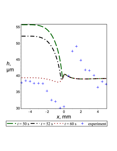
To study the formation of a patterned polymer coating during alcohol evaporation, a series of computational experiments were performed. From these, first of all, it is necessary to understand which mechanism plays the primary role: the thermal Marangoni flow, the capillary flow or the solutal Marangoni flow. To accomplish this, let us compare the results of two computations with the experimental data Cavadini et al. (2013). The first computation “A” takes into account the capillary flow and the thermal Marangoni flow (Fig. 4a). The solutal Marangoni flow and the capillary flow are taken into account in the second computation “B” (Fig. 4b). If capillary flow dominated, then both results would be similar but this is far from the case. We do not know what the residual fraction of liquid was when measuring the final film thickness Cavadini et al. (2013), therefore, Fig. 4 shows numerical results for several time points towards the end of the evaporation process. The comparison presented in Fig. 4b shows the qualitative similarity of the numerical computation results and the experimental data. This allows us to conclude that solutal Marangoni flow in the system under consideration plays a primary role. For this reason, the results presented below relate solely to computation “B”. Perhaps the quantitative match did not work out due to assuming when constructing the model, but the experimental data Cavadini et al. (2013) correspond to the value m/s in Fig. 4.
(a)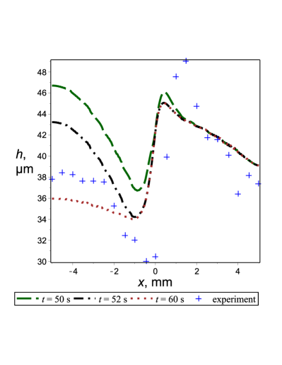 (b)
(b)
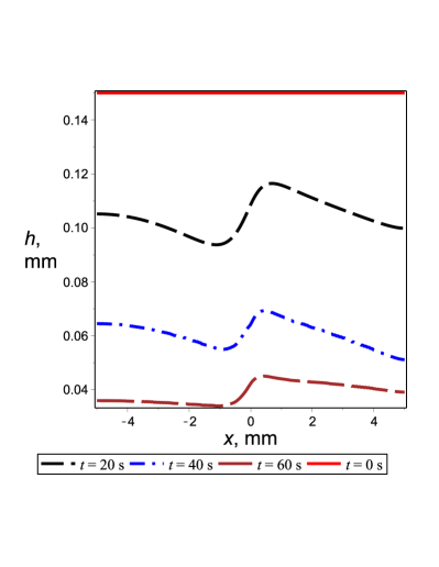
The shape of the free film surface for several consecutive time points is shown in Fig. 5a. In addition, for convenience, the spatiotemporal evolution of is shown in the form of a 3D plot (Fig. 5b). The shape of the free film surface at the initial time is flat. Further, during the evaporation, this surface shape becomes curved. The film height decreases over time as the liquid evaporates. As in the experiment Cavadini et al. (2013), reduction of in the Teflon region () can be observed, and thickening of this layer occurs in the aluminum region (). The fact is that the polymer weight increases over time in the aluminum region and decreases over the Teflon since the fluid flow transfers the admixture from the Teflon to the aluminum.
(a)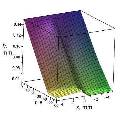 (b)
(b)
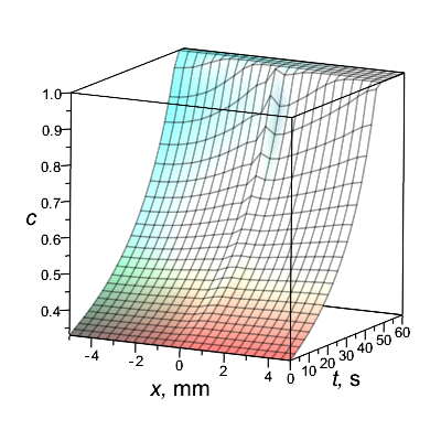
The polymer mass fraction increases with time above the aluminum faster than above the Teflon (Fig. 6). After the 50th second, not much fluid remains, and that which does is principally above the Teflon, that is, evaporation no longer occurs above the aluminum. By the 60th second of the process, evaporation stops completely since no alcohol remains in the system. At this moment, a solid patterned polymer film has formed. Around point a small bump may be noticed in the mass fraction value (Fig. 6), it is there that the valley is adjacent to the peak of (Fig. 4b).
The temperature calculation results indicate that the film (Fig. 7a) and substrate temperature (Fig. 7b) in the aluminum region remain almost unchanged over time. Aluminum has a relatively high thermal conductivity coefficient so the heat transferred by this material to the solution is quickly balanced by the environmental heat. The temperature in the region of the Teflon, which has a relatively low thermal conductivity, drops over time since evaporative cooling does not have time to be balanced by heat inflow from outside.
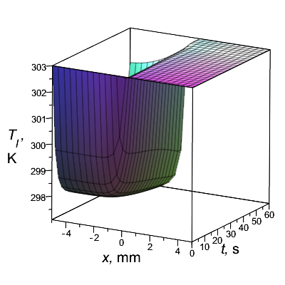
(a) (b)
(b)
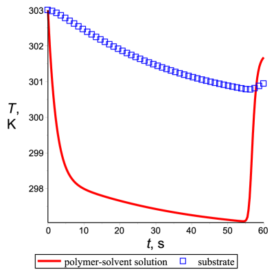
(a)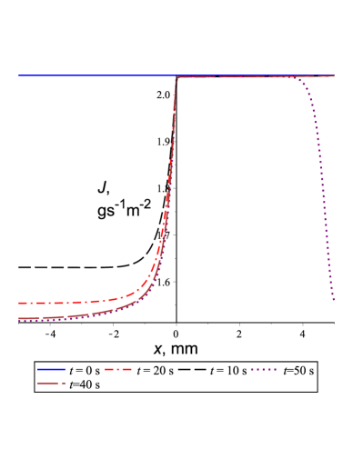 (b)
(b)
However, by the 55th second, the temperature gradient changes direction starting to rise (Fig. 8a). This is because the alcohol has almost completely evaporated around point by this time, resulting in the vapor flux density (Fig. 8b). The maximum temperature change of the film is about 6 K. In the case of the substrate, the maximum temperature change is approximately 2 K. Temperature dynamics affect the vapor flux density. At the process start (), the value 2.05 g/(m2s) is uniform along the free film surface (Fig. 8b), because the temperature is also distributed uniformly along the spatial coordinate (Fig. 7a). Later, the value decreases in the relatively cold region above the Teflon (). At the process end, the vapor flux density also starts to decrease in the region of the aluminum () since the polymer mass fraction value approaches 1.

The redistribution of polymer mass can be inferred by the curve of pressure (Fig. 9) exerted by this mass on the substrate by gravity (). The mass decreases over time above the Teflon layer and increases in the region of the aluminum surface. The reason for this is the convective mass transfer caused by the solutal Marangoni effect.
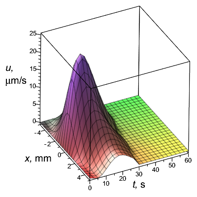
As can be seen from Fig. 10 the flow velocity initially increases over time. The solution flow is directed along the positive direction of the axis, from the Teflon layer to the aluminum surface. The maximum value of is reached at time 20 s in the point and is about 25 m/s. As this indicates the horizontal flow velocity averaged over the liquid layer height it should be understood that the solutal Marangoni flow velocity on the free film surface will be greater than this value. Subsequently, the velocity decreases reaching the value by about the 35th second i.e. the flow ceases. It follows that convective mass transfer occurs only during this period of time. At this point the solution concentration exceeds the critical value so the flow stops due to the high viscosity.
IV Conclusion
The results of the numerical computations indicate that solutal Marangoni flow plays a key role in the formation of a patterned polymer film as the methanol is lost during drying. This confirms the hypothesis of the authors of the practical experiment Cavadini et al. (2013). The results obtained here are in qualitative agreement with their experimental data. This study allows us to better understand the mechanisms that can be used in evaporative lithography.
The rapid heat transfer from the aluminum surface to the liquid results in this region being less cold than the Teflon coating region, meaning that, above the aluminum surface, the vapor flux density is greater. Due to the relatively rapid evaporation, the polymer concentration in that local region increases more strongly resulting in a significant increase in the surface tension coefficient. Accordingly, the solutal Marangoni flow is directed towards the aluminum surface along the free surface of the liquid film. This transfers even more polymer there. As a consequence, this additionally promotes a local increase in the polymer concentration in the solution and intensification of fluid flow affecting the admixture mass transfer. Thus, the Matthew effect emerges here. This flow increases until the viscosity begins to dominate. A further increase in viscosity due to an increase in the concentration of the solution leads to cessation of the flow.
The one-dimensional model described here is phenomenological in its nature. To obtain more accurate quantitative predictions a complex model should to be developed considering additional details such as the air flow velocity over the free film surface, , etc. In order to determine how the plate thickness affects the polymer film geometry a multidimensional model must be developed.
Acknowledgements.
This work is supported by Grant No. 22-79-10216 from the Russian Science Foundation (https://rscf.ru/en/project/22-79-10216/).Data Availability Statement
The data that support the findings of this study are available from the corresponding author upon reasonable request.
Appendix A Estimation of several problem parameters
The surface tension temperature gradient can be estimated using the empirical formula derived from the Eötvös rule, where the constant 2.1 g cm2/(s2 K mol2/3). Substituting the values of the liquid parameters (methanol density 0.792 g/cm3 and molar weight 32 g/mol) results in g/(K s2) and converting grams to kilograms provides the value , presented in Table 1.
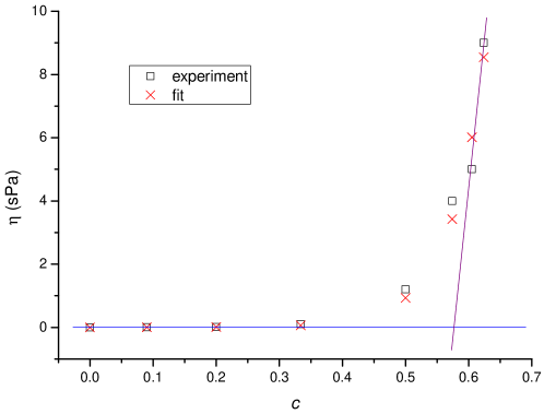
Fig. 11 shows the method for determination of the phase transition concentration (see Table 1). The experimental data are taken from the article Tönsmann, Scharfer, and Schabel (2021). Two main linear trends were determined, at the intersection of which the value was obtained.
The convective heat exchange coefficients are calculated as follows: and (see Table 1, 2) where the Nusselt numbers and Patochkina, Kazarinov, and Tkachenko (2016). The values of the empirical parameters were taken from Table 1 of Ref. Patochkina, Kazarinov, and Tkachenko (2016) (, ). The value for is taken from the article Gatapova et al. (2014) in accordance with the value (see Table 1).
Appendix B Derivation of equations based on the mass conservation law
Consider the mass balance of the solution in an elementary volume (Fig. 12). The left border of corresponds to the coordinate , and the right border corresponds to the coordinate . The upper boundary “air–liquid” is determined by the coordinate . The lower boundary “liquid–substrate” () is impermeable, thus there is no mass flux through it. The outflux of mass occurs through the upper boundary as a result of evaporation. In addition, the convective flow transfers the matter across the left and right boundaries of .
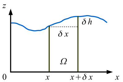
During , the mass of the solution in the volume will change due to changes in the volume itself and in the solution density,
| (6) |
where notation such as should be interpreted as . The mass flux density through the left and right (lateral) sides is written as . The length of the upper boundary is expressed as
where is the thickness difference of the film on the left and right borders of .
Let us take into account the area of the lateral sides, , and the area of the upper one, . The change in mass in during is associated with the transfer of mass through the lateral and upper boundaries,
| (7) |
Equate the right parts of the expressions (6) and (7), divide by , and get
As a result of the limit transition (, ), we come to the equation
| (8) |
it follows from the lubrication approximation that
Now let us consider the balance of the polymer mass in the elementary volume . During the time , the mass of the polymer changes by
| (9) |
This mass change is caused by convective and diffusive transport across the lateral boundaries of ,
| (10) |
where the diffusion flux density of the admixture is , this following from Fick’s law. Equate the right parts of (9) and (10), divide them by , and, as a result of the limiting transition, we obtain the convection–diffusion equation
Next, this equation is rewritten in the following form,
Divide the left and right sides of the equation by and taking into account (8) we get
In dimensionless form, this equation can be written as (3).
References
- Deegan et al. (1997) R. D. Deegan, O. Bakajin, T. F. Dupont, G. Huber, S. R. Nagel, and T. A. Witten, “Capillary flow as the cause of ring stains from dried liquid drops,” Nature 389, 827–829 (1997).
- Deegan (2000) R. D. Deegan, “Pattern formation in drying drops,” Physical Review E 61, 475–485 (2000).
- Sefiane (2014) K. Sefiane, “Patterns from drying drops,” Advances in Colloid and Interface Science 206, 372–381 (2014).
- Routh and Russel (1998) A. F. Routh and W. B. Russel, “Horizontal drying fronts during solvent evaporation from latex films,” AIChE Journal 44, 2088–2098 (1998).
- Harris et al. (2007) D. J. Harris, H. Hu, J. C. Conrad, and J. A. Lewis, “Patterning colloidal films via evaporative lithography,” Physical Review Letters 98, 148301 (2007).
- Harris and Lewis (2008) D. J. Harris and J. A. Lewis, “Marangoni effects on evaporative lithographic patterning of colloidal films,” Langmuir 24, 3681–3685 (2008).
- Kolegov and Barash (2020) K. S. Kolegov and L. Y. Barash, “Applying droplets and films in evaporative lithography,” Advances in Colloid and Interface Science 285, 102271 (2020).
- D'Ambrosio et al. (2023) H.-M. D'Ambrosio, S. K. Wilson, A. W. Wray, and B. R. Duffy, “The effect of the spatial variation of the evaporative flux on the deposition from a thin sessile droplet,” Journal of Fluid Mechanics 970 (2023), 10.1017/jfm.2023.503.
- Li, Kar, and Kumar (2019) T. Li, A. Kar, and R. Kumar, “Marangoni circulation by UV light modulation on sessile drop for particle agglomeration,” Journal of Fluid Mechanics 873, 72–88 (2019).
- Al-Muzaiqer et al. (2021a) M. A. Al-Muzaiqer, N. A. Ivanova, V. M. Fliagin, and P. V. Lebedev-Stepanov, “Transport and assembling microparticles via Marangoni flows in heating and cooling modes,” Colloids and Surfaces A: Physicochemical and Engineering Aspects 621, 126550 (2021a).
- Al-Muzaiqer et al. (2021b) M. A. Al-Muzaiqer, K. S. Kolegov, N. A. Ivanova, and V. M. Fliagin, “Nonuniform heating of a substrate in evaporative lithography,” Physics of Fluids 33, 092101 (2021b).
- Farzeena and Varanakkottu (2022) C. Farzeena and S. N. Varanakkottu, “Patterning of metallic nanoparticles over solid surfaces from sessile droplets by thermoplasmonically controlled liquid flow,” Langmuir 38, 2003–2013 (2022).
- Perkins-Howard et al. (2022) B. Perkins-Howard, A. R. Walker, Q. Do, D. I. Senadheera, F. Hazzazi, J. P. Grundhoefer, T. Daniels-Race, and J. C. Garno, “Surface wettability drives the crystalline surface assembly of monodisperse spheres in evaporative colloidal lithography,” The Journal of Physical Chemistry C 126, 505–516 (2022).
- Hegde et al. (2022) O. Hegde, R. Chatterjee, A. Rasheed, D. Chakravortty, and S. Basu, “Multiscale vapor-mediated dendritic pattern formation and bacterial aggregation in complex respiratory biofluid droplets,” Journal of Colloid and Interface Science 606, 2011–2023 (2022).
- Li et al. (2021) D. Li, R. Chen, X. Zhu, Q. Liao, D. Ye, Y. Yang, W. Li, H. Li, and Y. Yang, “Light-fueled beating coffee-ring deposition for droplet evaporative crystallization,” Analytical Chemistry 93, 8817–8825 (2021).
- Goy et al. (2022) N.-A. Goy, N. Bruni, A. Girot, J.-P. Delville, and U. Delabre, “Thermal Marangoni trapping driven by laser absorption in evaporating droplets for particle deposition,” Soft Matter 18, 7949–7958 (2022).
- Berneman et al. (2021) N. Berneman, I. Jimidar, W. V. Geite, H. Gardeniers, and G. Desmet, “Rapid vacuum-driven monolayer assembly of microparticles on the surface of perforated microfluidic devices,” Powder Technology 390, 330–338 (2021).
- Corletto and Shapter (2021) A. Corletto and J. G. Shapter, “Thickness/morphology of functional material patterned by topographical discontinuous dewetting,” Nano Select 2, 1723–1740 (2021).
- Gambaryan-Roisman (2010) T. Gambaryan-Roisman, “Marangoni convection, evaporation and interface deformation in liquid films on heated substrates with non-uniform thermal conductivity,” International Journal of Heat and Mass Transfer 53, 390–402 (2010).
- Gambaryan-Roisman (2012) T. Gambaryan-Roisman, “Marangoni-induced deformation of evaporating liquid films on composite substrates,” Journal of Engineering Mathematics 73, 39–52 (2012).
- Gambaryan-Roisman (2015) T. Gambaryan-Roisman, “Modulation of Marangoni convection in liquid films,” Advances in Colloid and Interface Science 222, 319–331 (2015).
- Iqbal et al. (2022) R. Iqbal, A. Matsumoto, D. Carlson, K. T. Peters, R. Funari, A. K. Sen, and A. Q. Shen, “Evaporation driven smart patterning of microparticles on a rigid-soft composite substrate,” Journal of Colloid and Interface Science 623, 927–937 (2022).
- Goel et al. (2019) P. Goel, M. D. Choudhury, A. B. Aqeel, X. Li, L.-H. Shao, and H. Duan, “Effect of thermal conductivity on enhanced evaporation of water droplets from heated graphene–PDMS composite surfaces,” Langmuir 35, 6916–6921 (2019).
- Zhao, Zhang, and Si (2023) C. Zhao, Z. Zhang, and T. Si, “Fluctuation-driven instability of nanoscale liquid films on chemically heterogeneous substrates,” Physics of Fluids 35 (2023), 10.1063/5.0159155.
- Cavadini et al. (2013) P. Cavadini, J. Krenn, P. Scharfer, and W. Schabel, “Investigation of surface deformation during drying of thin polymer films due to Marangoni convection,” Chemical Engineering and Processing: Process Intensification 64, 24–30 (2013).
- Ahlers and Xu (2001) G. Ahlers and X. Xu, “Prandtl-number dependence of heat transport in turbulent Rayleigh–Bénard convection,” Physical Review Letters 86, 3320–3323 (2001).
- Tönsmann, Scharfer, and Schabel (2021) M. Tönsmann, P. Scharfer, and W. Schabel, “Transient three-dimensional flow field measurements by means of 3D µptv in drying poly(vinyl acetate)-methanol thin films subject to short-scale Marangoni instabilities,” Polymers 13, 1223 (2021).
- Roubíček (2021) T. Roubíček, “From quasi-incompressible to semi-compressible fluids,” Discrete and Continuous Dynamical Systems - Series S 14, 4069 (2021).
- Kolegov (2018) K. S. Kolegov, “Simulation of patterned glass film formation in the evaporating colloidal liquid under IR heating,” Microgravity Science and Technology 30, 113–120 (2018).
- Cavadini et al. (2015) P. Cavadini, J. Erz, D. Sachsenheimer, A. Kowalczyk, N. Willenbacher, P. Scharfer, and W. Schabel, “Investigation of the flow field in thin polymer films due to inhomogeneous drying,” Journal of Coatings Technology and Research 12, 921–926 (2015).
- Sazhin (2006) S. S. Sazhin, “Advanced models of fuel droplet heating and evaporation,” Progress in Energy and Combustion Science 32, 162–214 (2006).
- Patochkina, Kazarinov, and Tkachenko (2016) O. L. Patochkina, Y. G. Kazarinov, and V. I. Tkachenko, “Physical model of the dependence of the nusselt number on the rayleigh number,” Technical Physics 61, 1626–1632 (2016).
- Gatapova et al. (2014) E. Y. Gatapova, A. A. Semenov, D. V. Zaitsev, and O. A. Kabov, “Evaporation of a sessile water drop on a heated surface with controlled wettability,” Colloids and Surfaces A: Physicochemical and Engineering Aspects 441, 776–785 (2014).