SAGAbg I: A Near-Unity Mass Loading Factor in Low-Mass Galaxies via their Low-Redshift Evolution in Stellar Mass, Oxygen Abundance, and Star Formation Rate

Abstract

Measuring the relation between star formation and galactic winds is observationally difficult. In this work we make an indirect measurement of the mass loading factor (the ratio between mass outflow rate and star formation rate) in low-mass galaxies using a differential approach to modeling the low-redshift evolution of the star-forming main sequence and mass–metallicity relation. We use the SAGA (Satellites Around Galactic Analogs) background galaxies, those spectra observed by the SAGA survey that are not associated with the main SAGA host galaxies, to construct a sample of 11925 spectroscopically confirmed low-mass galaxies from $0.01\lesssim z\leq 0.21$ and measure a auroral line metallicity for 120 galaxies. The crux of the method is to use the lowest redshift galaxies as the boundary condition of our model, and to infer a mass-loading factor for the sample by comparing the expected evolution of the low redshift reference sample in stellar mass, gas-phase metallicity, and star formation rate against the observed properties of the sample at higher redshift. We infer a mass-loading factor of $\eta_{\rm m}{}=0.92^{+1.76}_{-0.74}$, which is in line with direct measurements of the mass-loading factor from the literature despite the drastically different set of assumptions needed for each approach. While our estimate of the mass-loading factor is in good agreement with recent galaxy simulations that focus on resolving the dynamics of the interstellar medium, it is smaller by over an order of magnitude than the mass-loading factor produced by many contemporary cosmological simulations.

1 Introduction

Low-mass ($M_{\star}\lesssim 10^{10}M_{\odot}$) and dwarf ($M_{\star}\lesssim 10^{9}M_{\odot}$) galaxies are systems of interest for topics that range from stellar feedback to large-scale structure to the nature of dark matter. In the nearby Universe, ongoing surveys are working to map out the low-mass satellite population of galaxies like our Milky Way in an effort to systematically explore the effect of environment on low-mass galaxy evolution and the implication of extragalactic satellite populations on ideas of near-field cosmology (Geha et al., 2017; Mao et al., 2021; Carlsten et al., 2022). At larger scales, the low-mass end of the stellar-to-halo mass relation remains broadly unconstrained but necessary for a full understanding of cosmological structure formation (Grossauer et al., 2015; Leauthaud et al., 2020; Carlsten et al., 2021), the galaxy-halo connection (Nadler et al., 2020; Danieli et al., 2022), and the properties of dark matter (Nadler et al., 2021; Newton et al., 2021). The number densities and density profiles of the dwarfs also have the potential to shed light on the nature of dark matter (see, e.g. Governato et al., 2012; Del Popolo & Pace, 2016; Bullock & Boylan-Kolchin, 2017; Nadler et al., 2020). On galactic scales, it has long been thought that the structure and evolution of dwarf galaxies are expected to be more sensitive to the nature of star formation feedback than are their massive counterparts, making these small systems important observational probes of our understanding of feedback and the baryon cycle (see, e.g. Dekel & Silk, 1986; White & Frenk, 1991; Dalcanton, 2007; Geha et al., 2012; Oñorbe et al., 2015; El-Badry et al., 2016; Wetzel et al., 2016; Hu, 2019; Semenov et al., 2021; Kado-Fong et al., 2022a, b; Jahn et al., 2022).

Star formation and the (self-)regulation thereof are thought be a crucial driver of structure and evolution in low-mass galaxies (Kim & Ostriker, 2018; Hu, 2019; Steinwandel et al., 2022a, b), but quantifying the impacts of the star formation cycle on individual galaxies is difficult due to the stochastic and temporally variable nature of star formation. A crucial component of the self-regulation of star formation is the ability of star formation to remove mass from the gas reservoir of the gas galaxy not only through conversion of gas to stars, but via galactic-scale outflows driven by star formation feedback (see, e.g. Lynden-Bell, 1975; Pagel & Patchett, 1975; Carigi, 1994; Lilly et al., 2013; Muratov et al., 2015; Anglés-Alcázar et al., 2017; Kim & Ostriker, 2018; Hu, 2019; Nelson et al., 2019; Pandya et al., 2020, 2021; Carr et al., 2022; Ostriker & Kim, 2022; Steinwandel et al., 2022a, b, 2023). The mass-loading factor, $\eta_{\rm m}$, is a key metric of star formation feedback that quantifies the amount of gas mass lifted out of a galaxy’s interstellar medium (ISM) per unit star formation, i.e.:

$$\eta_{\rm m}{}\equiv\frac{\dot{M}_{\rm out}}{\text{SFR}},$$ (1)

where $\dot{M}_{\rm out}$ is the rate of mass outflow from the galaxy. Crucially for this work, the mass-loading factor is thought to play a key role in setting the mass–metallicity relation by controlling the flow of metal-enriched gas out of the ISM.

To measure a mass outflow rate one must determine both the location of the gas (i.e. that the relevant gas has been lifted out of the galaxy) and the speed of the gas (to estimate the rate at which the gas is flowing out of the host galaxy). Due to the projected nature of extragalactic astronomy, it is often difficult to measure both the distance from the midplane $z$ (or $r$) and outflow velocity $v_{z}$ (or $v_{r}$). Even when both position and velocity can be measured (Marasco et al., 2023), the complex dynamical state of the gas reservoirs in low-mass galaxies make the interpretation of their kinematics – and thus the estimation of the mass-loading factor – a complex task. Deriving an estimate of a total mass density from observable quantities of specific lines is also subject to uncertainties due to assumptions regarding ionization and abundance corrections. One either observes that the gas has been displaced but not the speed of the displaced gas (McQuinn et al., 2019) or observes the velocity of the gas but not its position (Martin, 1999; Heckman et al., 2015; Chisholm et al., 2017; Marasco et al., 2023).

Another approach to constraining the mass-loading factor is to determine the range of mass-loading factors that are permissible given the current state of the mass metallicity relation or other scaling relations (Lilly et al., 2013; Lin & Zu, 2023). Using the chemical enrichment history of individual or sets of galaxies is a well-established method of modeling their gas cycling processes due to the inherent link between a galaxy’s gaseous and stellar content (see, e.g. Lynden-Bell, 1975; Pagel & Patchett, 1975; Carigi, 1994; Matteucci, 2016; Maiolino & Mannucci, 2019; Matteucci, 2021). The difficulty with this more indirect approach is that the mass-loading factor is not the sole parameter that sets the mass–metallicity relation at $z\sim 0$ and some degree of complexity is required to instantiate $z\sim 0$ observations; these models have nevertheless been successful in establishing mass-loading factor estimates across a large range of stellar masses (see, for example, Bouché et al., 2010; Yin et al., 2011; Davé et al., 2012; Lilly et al., 2013; Yin et al., 2023).

In this work, we adapt the indirect method of estimating the mass-loading factor via its effect on the low-redshift ($z\lesssim 0.2$) evolution of both the star-forming main sequence and mass–metallicity relations. Rather than taking on the substantial hurdle of producing a realistic $z\sim 0$ galaxy population, we will use our observed lowest redshift galaxy sample as our $z=0$ boundary condition.

This approach differs from classic literature methods in its intrasample differential nature, where we will explicitly model the selection function of a single sample rather than making a multi-sample comparison (as in, e.g. Zahid et al., 2012), and by using the lowest redshift galaxies in our sample as a tautologically realistic boundary condition for our method (as opposed to full-fledged regulator models such as Lilly et al., 2013). Here, the size and depth of our sample allow us to explicitly characterize the selection function of the SAGA background galaxy sample to enable modeling of chemical evolution on an intrasample basis. The method allows us to partially circumvent the well-known issue of absolute calibrations in gas-phase metallicity estimates (Kewley & Ellison, 2008; Kewley et al., 2019), directly account for photometric and spectroscopic incompleteness during model comparison, and use measured star formation rates (SFRs) as model inputs rather than predicting SFR via star formation efficiency arguments.

In order to execute this approach, we need a large spectroscopic sample of low-mass galaxies out to a sufficiently large redshift such that some physical evolution of the population is expected to be detectable. The Satellites Around Galactic Analogs (SAGA) background galaxies provide such a sample. Although the main science driver of the SAGA Survey is a census of satellite galaxies around Milky Way-like hosts, the vast majority of the spectra collected are of low-mass galaxies at somewhat higher redshift. The SAGA sample sits in the wider context of efforts that have been put into cataloging the dwarf galaxy population within the Local Volume and nearby Universe (Dale et al., 2009; Lee et al., 2009a, b; Berg et al., 2012; Hunter et al., 2012; Cook et al., 2014). New and ongoing surveys are now systematically mapping out the low-mass galaxy population at $z>0$ (Darragh-Ford et al., 2022; Luo et al., 2023), which has borne out new possibilities for understanding the broader population of dwarf galaxies and contextualizing our Local Volume on a wider scale.

We will argue that the SAGA galaxies imply an average mass-loading factor of $\eta_{\rm m}\sim 1$ at $10^{7.5}\lesssim M_{\star}/M_{\odot}\lesssim 10^{9.5}$, in agreement with observational measures of the mass-loading factor of individual galaxies and inconsistent with recent simulations that call for large mass-loading factors at low mass in order to produce realistic $z=0$ dwarfs.

We adopt a flat $\Lambda$CDM cosmology with $\Omega_{m}=0.3$ ($\Omega_{\Lambda}=0.7$), and $H_{0}=70\ {\rm km\ s^{-1}}{}\ {\rm Mpc^{-1}}$. We use a Kroupa (2001) initial mass function (IMF) unless otherwise specified, and convert literature results that use other IMFs to a Kroupa (2001) IMF as stated in the text.

2 SAGAbg-A and the SAGA Background Galaxies

The SAGA Survey is a spectroscopic search for satellites down to $M_{r}\sim-12$ around MW-like hosts at $z\sim 0.01$ (Geha et al., 2017; Mao et al., 2021). Due to the rarity of the satellite galaxies, the significant majority of spectra collected by SAGA are galaxies that are not associated with the SAGA hosts, in order to reach a highly complete survey. Nevertheless, these non-satellite (background) galaxies tend to be low-redshift and relatively low-mass due to the photometric selection used by SAGA (Mao et al., 2021).

These background spectra represent a sample of primarily low-mass galaxies down to a limiting magnitude of $m_{r}\sim 21$, a magnitude fainter than the Galaxy And Mass Assembly survey(GAMA, Baldry et al., 2010) with effective exposure times around twice as long. The SAGA background spectra thus provide a fainter and deeper look into the low-redshift, low-mass galaxy population than has been possible with previous generation spectroscopic surveys.

In this work, we consider a subset of SAGA background galaxies which we will call the SAGAbg-A sample. The nomenclature simply refers to the galaxies’ status as background galaxies (bg), and that this is the first subset of the background galaxies used for science (-A). The SAGAbg-A sample only includes galaxies for which spectra were either drawn from archival SDSS or GAMA observations or obtained with AAT/2dF or MMT/Hectospec during the SAGA spectroscopic campaign, and excludes the satellites of the SAGA hosts themselves (i.e., the main science targets of the SAGA Survey). The SAGAbg-A sample considered covers an on-sky area of around 110 sq. deg., though as we will discuss in Section 4 the spatial coverage over this area is not uniform. The data set includes the data presented in Geha et al. (2017) and Mao et al. (2021), as well as additional survey data that will be presented in a forthcoming work (Mao et al., in preparation).

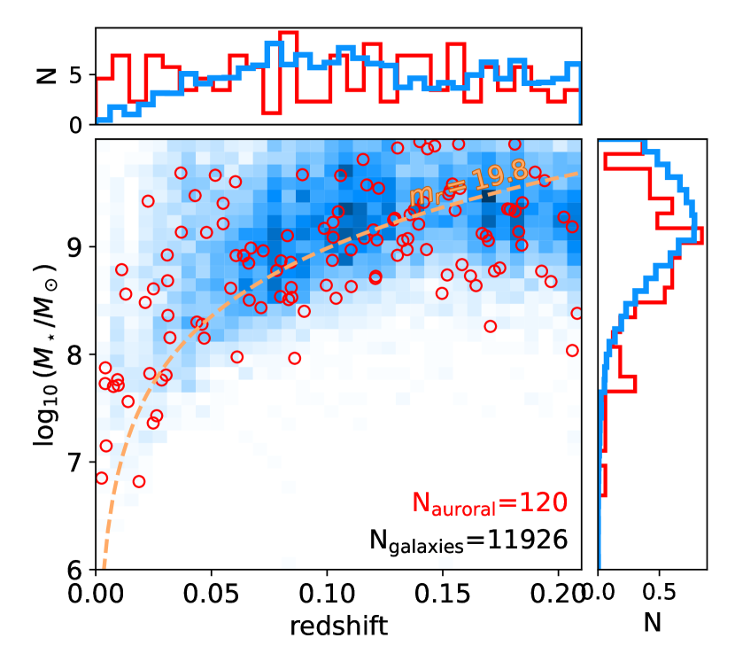
Figure 1: The distribution of the SAGAbg-A sample in redshift and stellar mass; we restrict our sample to those galaxies with stellar masses $\log_{10}(M_{\star}/M_{\odot})$$<10$ and $z<0.21$. Unfilled red circles show galaxies for which we can measure weak auroral line metallicities, as will be presented in detail in Section 2.2. The top and right panels show the projection of the distribution over stellar mass and redshift, respectively, for both the full (blue) and auroral line-detected (red) samples. In the main panel, the gold dashed curve shows the stellar mass corresponding to an apparent magnitude of $m_{r}=19.8$ assuming $(g-r)=0.3$, which corresponds to the limiting magnitude of the majority of GAMA spectroscopic fields.

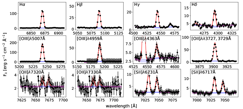
Figure 2: An example spectrum fit for a galaxy at $z=0.047$ (RA=11h16m05.2s, Dec=+48d20m15.1s), showing fits to different emission lines. Note that the redder O II weak lines are not fit for the galaxy as they are redshifted beyond 8000 Å. In each panel, the top left label indicates the emission line of interest. Black points show observed specific flux, while the red curve shows the best-fit model. The blue curve shows the same best-fit model without emission (i.e., showing only stellar absorption and continuum).

Figure 3: The same as Figure 2, but showing only the key weak auroral lines ([O III]$\lambda$4363Å and [O II]$\lambda$7320Å,[O II]$\lambda$7330Å) and their strong line counterparts for three galaxies at different redshifts. Note that in the highest redshift example shown here (bottom row), the O II auroral lines are redshifted out of the spectrum wavelength range and are hence not shown. The galaxies shown are at (RA=11h16m05.2s, Dec=+48d20m15.1s; RA=21h39m13.5s, Dec=-42d35m07.3s, RA=13h46m56.4s, Dec=+41d54m26.0s).

2.1 Photometric Selection

The photometric selection of the SAGA Survey is designed to completely span the range of photometric properties occupied by the SAGA satellites, which are low-mass ($\log_{10}(M_{\star}/M_{\odot})$$\lesssim 10$) galaxies at $z\lesssim 0.013$. As the SAGA Survey progressed, the photometric selection has evolved to exclude more background galaxies while maintaining the completeness of satellite galaxies (Geha et al., 2017; Mao et al., 2021). As such, when we consider the SAGA background galaxies, their effective photometric selection is not uniform across different SAGA hosts. Because we are interested only in the galaxies not associated with the SAGA hosts, however, we argue that it is sufficient to characterize the realized aggregate selection function of the SAGA background galaxies.

The SAGA host fields, when the satellites themselves are excluded, can be considered to be random fields. Since there should be no differences in the population of galaxies between two random fields, there should also be no difference – modulo cosmic variation – between targeting each random field with somewhat different photometric cuts and targeting all fields with the average photometric cuts as weighted by number of spectra obtained using each selection function.

Taking this aggregate approach allows us to characterize the SAGAbg-A sample by its effective photometric selection, which we will quantify as the fraction of SAGA photometric targets that are in the SAGAbg-A sample (we remind the reader that this is not equivalent to the fraction of galaxies with a SAGA redshift). Our model is built around the idea that our sample is incomplete, and that we can quantify our incompleteness relative to some “most complete” subset. We will return to this idea more quantitatively in Section 4 when we build a model to understand the physical evolution of our observed samples.

While we defer a full characterization of this aggregate selection function and its impact on the present sample to Section 4, we would like to acquaint the reader with the sample at hand we show in Figure 1 the distribution of the sample over redshift and stellar mass. The stellar mass that would correspond to an apparent magnitude of $m_{r}=19.8$ for a galaxy with a restframe color of $(g-r)=0.3$ using our color-mass relation as an orange curve. This apparent magnitude is roughly equal to the limiting magnitude of most field in the Galaxy Mass and Assembly (GAMA) survey (Driver et al., 2009).

2.2 SAGA Spectra

Measuring star formation rates from H$\alpha$ luminosities and gas-phase metallicites from temperature-sensitive oxygen line flux ratios requires flux-calibrated spectra. As mentioned earlier, the SAGAbg-A sample used in this work includes all spectra obtained from MMT/Hectospec and AAT/2dF (including GAMA archival spectra), as well as all archival spectra of SAGA photometric targets taken by SDSS.

We find that the relative flux calibration of the SAGA AAT and MMT spectra, particularly those spectra from AAT/2dF, degrades at $\lambda\gtrsim 8000$ Å. This cutoff was determined by comparing SAGA spectra to spectra of the same galaxies released by the GAMA survey; we deem the SAGA flux calibration unreliable when the fractional difference $f(\lambda)\equiv|F_{\lambda}^{\rm SAGA}(\lambda)-F_{\lambda}^{\rm GAMA}(\lambda)|/\sqrt{\sigma_{F_{\lambda}}^{\rm SAGA}(\lambda)^{2}+\sigma_{F_{\lambda}}^{\rm GAMA}(\lambda)^{2}}$ between the SAGA and GAMA flux calibration reaches $f(\lambda_{\rm cut})>2$ and the sign of $df/d\lambda$ is constant at $\lambda>\lambda_{\rm cut}$. We thus cut off the spectra in our analysis at $\lambda{{\color[rgb]{0,0,0}{}_{\rm cut}}}=8000$ Å for spectra originating from AAT/2dF and $\lambda{{\color[rgb]{0,0,0}{}_{\rm cut}}}=8200$ Å for MMT/Hectospec. We note that the spectra obtained by SAGA have an average integration time of 2 hours on the 3.9m AAT and 1.5 hours on the 6.5m MMT and comprise the vast majority (94%) of the final sample.

Next, we flux calibrate our spectra using the SAGA $g-$ and $r-$band photometry by assuming that the spectrum is representative of the full galaxy (i.e. assuming that there are no underlying population gradients) and applying the multiplicative conversion to reproduce the SAGA photometry from integrating the SAGA spectrum. This method is well-suited for our sample because the galaxies are generally small even compared to the relatively small AAT/2dF and MMT/Hectospec fibers: the median on-sky effective radius of our sample is 1.2″, while the AAT/2dF and MMT/Hectospec fibers are 2.1″ and 1.5″ in diameter, respectively. Because the $g-$ and $r-$bands lie on different AAT/2dF spectrograph arms, we allow for different flux calibrations in $g$ and $r$ for AAT/2dF spectra to correct for any discontinuities between the two arms that persisted beyond relative flux calibration. Finally, because the relative flux calibration is quite important for our metallicity measurements, we remove any AAT/2dF spectra that contain a discontinuity of greater than 5% across the spectrograph break after absolute flux calibration.

We apply flux calibration to the SDSS spectra in the same way that we do for the SAGA AAT and MMT spectra. The flux calibration provided by the GAMA public data release are already calibrated consistently to our flux calibration and so we do not perform an additional flux calibration. For all spectra we correct for galactic extinction assuming a Cardelli et al. (1989) extinction curve with an assumed $R_{V}=3.1$ and the galactic $A_{V}$ measured by Schlafly & Finkbeiner (2011) at the position of each target via the IRSA galactic dust and reddening server (IRSA, 2022).

3 Measurements

In this work, we will infer weak line ratios and strong line fluxes of the SAGAbg-A spectra, convert those line measurements to estimates of ISM physical conditions, and use those physical conditions to make an inference about the evolution of the galaxy sample over a short period of cosmic time (e.g. lookback times of less than $t_{lb}$$\lesssim 2.5$ Gyr). Throughout this process, we will leverage our external knowledge (e.g. of atomic physics, of the sample selection) to make an inference of the system as a whole rather than independently estimating parameters from individual components of our data.

We will measure gas-phase metallicities for the sample using the “electron temperature” approach, which uses temperature-sensitive weak line ratios to constrain the temperature (and thus the emissivity) of O II and O III-emitting gas. The quality of the SAGA spectra allows us to confidently measure these key auroral line fluxes ([O III]$\lambda$4363Å, [O II]$\lambda$7320Å, and [O II]$\lambda$7330Å) for a small but significant fraction of the galaxy sample. These line ratios are strongly temperature-dependent and density-insensitive (for the densities relevant to this work). Auroral line metallicities are often thought of as “gold standard” metallicities because ion abundance can be directly computed from flux ratios (e.g. of [O III]$\lambda$5007Å/H$\beta$) once the temperature and density (and thus the line emissivities) are measured from temperature-sensitive line ratios. However, it is important to note that auroral line metallicities also suffer from biases. The most often-used auroral line [O III]$\lambda$4363Å is rarely seen at metallicities exceeding $\log_{10}\text{(O/H)}+12=8.7$ — this bias is mitigated by the low metallicity of our sample (for a recent review, see Kewley et al., 2019). It is also known that auroral line metallicity samples tend to preferentially select metal-poor galaxies (Kewley & Ellison, 2008), and that samples selected to have [O III]$\lambda$4363Å detections can result in an underestimate of the mass-metallicity relation (Curti et al., 2020). Furthermore, the impact of temperature and density inhomogeneities on $T_{e}$-based metallicity estimates remains an open question at both the H II region and galactic scale (Chen et al., 2023; Méndez-Delgado et al., 2023a, b).

Nevertheless, we find that it is preferable to compare auroral line metallicities across cosmic time than to compare either empirical calibrations of strong line ratios or theoretical metallicity calibrations. The former regularly show mean offsets of 0.5–1.0 dex between theoretical calibrations of the same strong line ratio, and the latter’s fidelity relies on our uncertain understanding of stellar atmospheres, evolution, and other model assumptions. In Appendix C, we rerun our analysis using various strong line metallicity calibrations from the literature and find that the conclusions are robust against choices of metallicity calibrator that accurately reproduces the known mass-metallicity relation of low-mass galaxies in the nearby Universe.

3.1 Line Measurements

The first step to measuring gas-phase metallicities is to measure fluxes of the relevant lines in our sample. The most important lines for our analysis in this paper series are H$\alpha$, H$\beta$, [O III]$\lambda$4363Å, [O III]$\lambda$5007Å, [O II]$\lambda\lambda$3727,3729Å, [O II]$\lambda$7320Å, and [O II]$\lambda$7330Å. We also fit a wider set of lines including the density-sensitive pair [S II]$\lambda$6717Å and [S II]$\lambda$6731Å. We show an example of a SAGA spectrum around the emission lines of interest in Figure 2 and several examples of the key weak auroral lines in galaxies across the redshift range of our sample in Figure 3. A full accounting of the lines fit for this analysis will be provided as a value-added catalog in a forthcoming work (Mao et al., in preparation).

We fit our emission lines and Balmer absorption features simultaneously; we allow the amplitude and position to vary for each line but assume that all the emission lines can be well-described by a Gaussian profile of the same width $\sigma_{em}$. The Balmer absorption features are also fit as an ensemble of Gaussian profiles wherein we require that the ratio between the equivalent width of each absorption feature and the equivalent width of the H$\beta$ absorption feature is held to be unity for H$\gamma$ and H$\delta$, and 0.5 for H$\alpha$ (i.e. $\rm EW_{H\alpha}=0.5EW_{H\beta}$). This relationship is chosen based on the models of González Delgado et al. (1999); we adopt a strict assumption here because the H$\alpha$ absorption is not spectrally resolved and is therefore degenerate with the emission component. We approximate the continuum local to each emission line as a constant value, and hold the continuum flux of lines separated by less than 140Å to be equal. We infer the properties of the all the emission line profiles in each SAGA spectra simultaneously via the Markov Chain Monte Carlo ensemble sampler implemented in emcee (Foreman-Mackey et al., 2013).

Our approach allows us to straightforwardly incorporate our knowledge of atomic physics into the line profile fitting by including this information into our formulation of the prior. In particular, we have strong constraints on the minimum allowable flux ratio of lines originating from the same species wherein the redder line is in the numerator. As an example, consider the flux ratio between H$\alpha$ and H$\beta$, i.e., the Balmer decrement. For a gas at $n_{e}$$=10^{3}$ cm^-3 and $T_{e}$$=10^{4}$ K, the intrinsic flux ratio between H$\alpha$ and H$\beta$ should be 2.86. In the presence of reddening from dust, the observed flux ratio may be larger than this value (but not smaller). We thus adopt a sigmoid prior

$$\rm Pr(A_{H\alpha},A_{H\beta})=(1+e^{-k(A_{H\alpha}/A_{H\beta}-\tilde{A}_{H\alpha,H\beta}b)})^{-1}$$ (2)

where $k=30$ and $b=0.925$ are the shape parameters of the sigmoid function, $\tilde{A}_{H\alpha,H\beta}$ is the intrinsic flux ratio (here assumed to be 2.86), and $\rm A_{H\alpha}$ and $\rm A_{H\beta}$ are the amplitudes of the H$\alpha$ and H$\beta$ lines, taking advantage of the fact that the ratio of the fluxes will be equal to the ratio of the amplitudes when the linewidth is equal. Note that the prior allows for, but is weighted against, line ratios somewhat below the assumed minimum intrinsic ratio. The same exercise can be performed with the other lines in the spectrum; we assume sigmoid priors with the following assumed intrinsic ratios:

• $\tilde{A}_{H\alpha,H\gamma}=6.11$

• $\tilde{A}_{H\alpha,H\delta}=11.06$

• $\tilde{A}_{[OIII]5007,[OIII]4959}=2.98$

• $\tilde{A}_{[OIII]5007,[OIII]4363}=6.25$

• $\tilde{A}_{[SII]4077,[SII]4069}=6.25$,

based on the minimum intrinsic line ratio for a reasonable ($10^{2}\lesssim T\lesssim 10^{5}$ K) range in temperature as computed by the package pyneb.

We adopt a simple Gaussian likelihood over our model parameters:

$$\ln\mathcal{L}(\vec{F}_{\lambda}|\vec{\theta}_{\ell})=-\frac{1}{2}\sum_{i}{\left[\frac{{\left(\hat{F}_{\lambda}(\lambda_{i},\vec{\theta}_{\ell})-F_{\lambda,i}\right)}^{2}}{\sigma_{F_{\lambda,i}}^{2}}+\ln{\left(2\pi\sigma_{F_{\lambda},i}^{2}\right)}\right]},$$ (3)

where the index refers to the index of the resolution element, $\hat{F}_{\lambda}(\lambda_{i})$ and $F_{\lambda,i}$ are the predicted and observed specific fluxes in that resolution element, respectively, and $\sigma_{F_{\lambda}}$ is the uncertainty in the specific flux. The observed spectrum is thus simply $\vec{F}_{\lambda}=\{F_{\lambda,0},F_{\lambda,1}...F_{\lambda,M}\}$ for $M$ resolution elements. The vector $\vec{\theta}_{\ell}$ is of length $2N_{\rm em}+N_{\rm cont}+3$; $\vec{\theta}_{\ell}$ describes the parameters of the line model. Here $N_{\rm em}\leq 18{}$ is the number of emission lines fit and $N_{\rm cont}\leq 10$ is the number of continuum regions fits. The numbers here are given as upper limits because lines that are redshifted beyond $\lambda=8000\text{ \AA}$ are excluded from the model. There are then an additional three parameters: $\sigma_{\rm em}$, the width of the emission lines, $\text{EW}_{\rm abs}$, the equivalent width of the Balmer lines, and $\sigma_{\rm abs}$, the width of the (Balmer) absorption lines. We show an example of our line-fitting procedure for a single galaxy in Figure 2, and several examples of the key O II and O III lines we use to estimate gas-phase metallicities across the sample redshift range in Figure 3.

Because some of the lines that we fit are quite weak (at maximum $\sim 10\%$ the flux of H$\alpha$ and [O III]$\lambda$5007Å), we visually inspect each galaxy in which the inference predicts a less than 16% chance that the auroral oxygen lines could originate from stochastic fluctuations to ensure that the measured features are not observational artifacts such as residuals from sky subtraction. Finally, in Appendix A we test both our flux calibration and line measurement methods against published GAMA survey results to verify that our methodology is consistent with established literature methods.

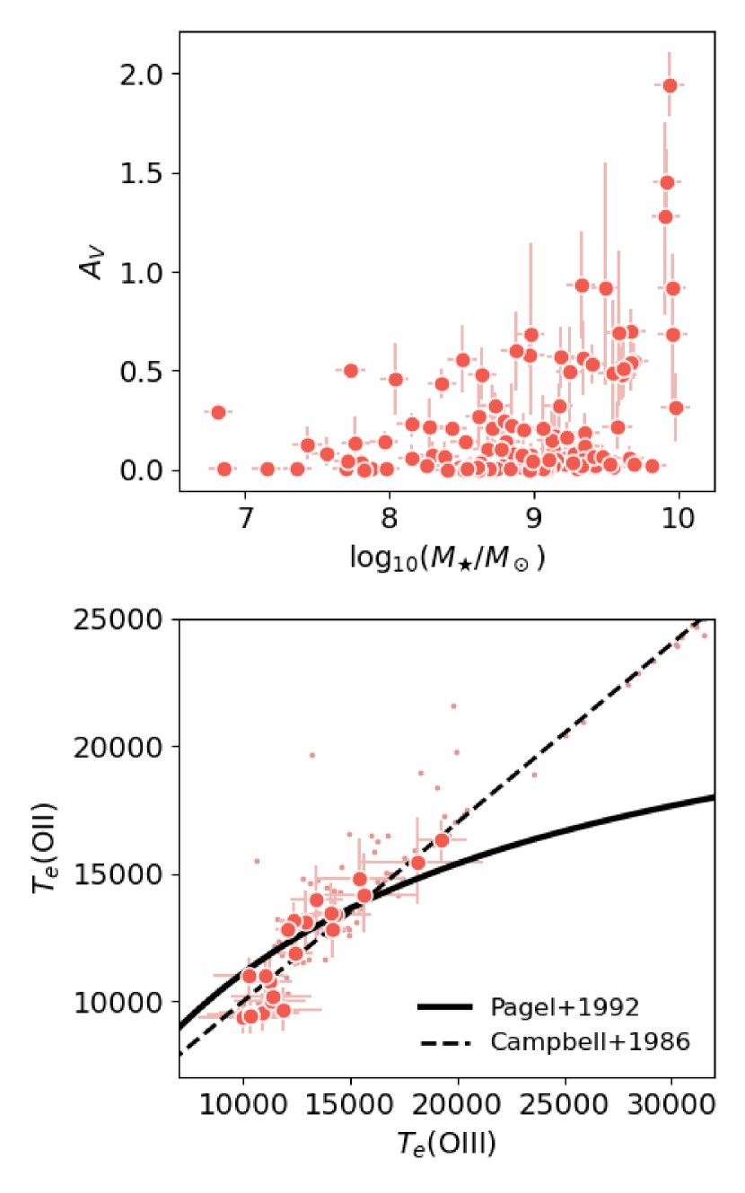
Figure 4: Top: stellar mass versus internal visual extinction ($A_{V}$) for the sample of galaxies for which we could measure a reliable auroral line metallicity. Bottom: $T_{e}$(O III) versus $T_{e}$(O II), where large points with error bars show galaxies where the auroral lines [O II]$\lambda$7320Å and [O II]$\lambda$7330Å are covered by the portion of the spectra with a reliable flux calibration and a strong detection (probability of being drawn from a blank spectrum $<0.05$) of at least one of the red auroral O II lines is present. Small scatter points indicate galaxies for which a weak auroral line metallicity could be measured from [O III]$\lambda$4363Å, but for which the O II lines were outside the rest-frame wavelength coverage of the SAGA spectrum. These galaxies are expected to follow the assumed prior temperature relation much more closely, though upper limits on [O II]$\lambda$7320Å and [O II]$\lambda$7330Å may still provide information that causes the estimate of $T_{e}$(O II) to deviate from the mean value assumed by the prior relation of Campbell et al. (1986, dashed line).

3.2 Determining ISM conditions

Line emissivity coefficients are generally a function of temperature ($T_{e}$) and density ($n_{e}$); thus, to invert line flux ratios to abundance ratios, we need to know the physical condition of the gas that is emitting the lines. Similar to our approach to measuring line fluxes, we will infer our ISM conditions of interest ($T_{e}$(O III), $T_{e}$(O II), and $A_{V}$) simultaneously via Markov Chain Monte Carlo sampling implemented from emcee. We additionally adopt a Calzetti et al. (2000) extinction curve and note that the best-fit extinction in these galaxies tends to be low, with $A_{V}<0.5$, which is unsurprising given their low stellar masses (see Figure 4).

A common method to estimate $T_{e}$ is to use the auroral [O III]$\lambda$4363Å line to leverage the temperature-sensitivity and density-insensitivity of the [O III]$\lambda$4363Å/[O III]$\lambda$5007Å flux ratio. This allows us to estimate the average $T_{e}$ probed by O⁺⁺, which we will follow the literature in calling the “high ionization” (O⁺⁺) zone electron temperature. However, H II regions are not typically isothermal — the average temperature that O⁺⁺ lines probe is not necessarily the same as the average temperature that O⁺ lines probe. To constrain the overall oxygen abundance, then, one needs a constraint on both $T_{e}$(O III) and $T_{e}$(O II). A relation between the high-ionization and “low-ionization” (O⁺) zones is often adopted (Berg et al., 2012). However, these relations are based on photoionization models of H II regions (Stasińska, 1990), and different models give different relations between the effective $T_{e}$ of each species (see, e.g. Campbell et al., 1986; Stasińska, 1990; Pagel et al., 1992).

Fortunately, there are also temperature-sensitive O II line ratios that can provide a more direct constraint on $T_{e}$(O II), though we note that these line ratios do have a moderate dependence on density (Hägele et al., 2006; Pérez-Montero, 2017). These are [O II]$\lambda$7320Å/[O II]$\lambda\lambda$3727,3729Å and [O II]$\lambda$7330Å/[O II]$\lambda\lambda$3727,3729Å. Unfortunately, these lines are close to our red wavelength cutoff (8000Å) even at $z=0$ and pass out of our redshift range at $z=0.09$. Additionally, at low SNR it is not guaranteed that both [O III]$\lambda$4363Å and the pair of weak O II lines will yield high-confidence detections. To account for either missing coverage or marginal detections, instead of measuring $T_{e}$(O III) and $T_{e}$(O II) independently we adopt a prior over their relationship based on the model prediction of Stasińska (1990):

$$\text{$T_{e}$({O~{}II})}\sim\mathcal{N}(0.7\ \text{$T_{e}$({O~{}III})}+\text{T}_{0},\sigma_{\text{$T_{e}$}}^{2}),$$ (4)

where $\text{T}_{0}=3000\text{ K}$ and we assume $\sigma_{\text{$T_{e}$}}=1500\rm\ K$. Here, $\mathcal{N}(\mu,\sigma^{2})$ denotes a normal distribution with mean $\mu$ and variance $\sigma^{2}$. We have also performed the same inference using the temperature relation of Pagel et al. (1992) and found that while our assumption for the form of the prior does result in different estimates of $T_{e}$(O II) when [O II]$\lambda$7220Å and [O II]$\lambda$7330Å are not covered, it does not significantly change our final metallicity estimates given the uncertainty on the posterior distribution of gas-phase metallicities.

We adopt uniform priors over $T_{e}$(O III) and $A_{V}$:

$$\begin{split}\text{$T_{e}$({O~{}III})}&\sim\mathcal{U}(5\times 10^{3},4\times 10^{4})\ {\rm K}\\ A_{V}&\sim\mathcal{U}(0,\infty),\end{split}$$ (5)

where the bounds on the former are set by the range of $T_{e}$(O III) seen in high-SNR measurements of individual H II regions in low-mass galaxies by Berg et al. (2012).

We would also like to constrain the density associated with the line emission, $n_{e}$. However, the density-sensitive line ratio that we have access to is from S II ([S II]$\lambda$6717Å/[S II]$\lambda$6731Å), and is only sensitive down to $n_{e}$$\sim 10^{2}$ cm^-3. We have run a version of this inference with $n_{e}$ allowed to vary and the S II lines included, and find in practice that our sample is consistent with the 100 cm^-3 low-density limit. This is in line with previous works over similar mass ranges (Berg et al., 2012; Andrews & Martini, 2013), so we choose to adopt $n_{e}$$=10^{2}$ cm^-3 for this work to avoid propagating the uncertainty of the S II density estimate without adding additional information to the inference. We also find that the inclusion of density as a free parameter does not significantly affect our inference of $T_{e}$(O II) despite the density dependence of the indicator line ratio. This is likely both because the O II line ratio is more sensitive to temperature than density over the densities probed, and because the overall oxygen abundance is expected to be dominated by doubly-ionized oxygen at these metallicities (Curti et al., 2017).

Here we use the posteriors of the line-fitting inference to construct a likelihood via density estimation. In particular, we estimate the probability density function of our line ratios of interest from the posterior distributions over line fluxes obtained in the previous section via a Gaussian kernel density estimate. We perform the density estimation independently for each of the line ratios considered; the likelihood is then simply the product of the estimated likelihood for each line ratio. For each line ratio considered, we first compute the line ratio predicted from the corresponding $T_{e}$ using the flux ratios computed using pyneb using the transition probabilities and temperature-dependent collision strengths reported by Storey & Zeippen (2000) and Storey et al. (2014) for O III, Zeippen (1982) and Kisielius et al. (2009) for O II, and Pequignot et al. (1991) and Storey & Hummer (1995) for H recombination. We then apply differential reddening assuming a Calzetti et al. (2000) extinction curve with an assumed $R_{V}=4.05$ to determine the expected observed line ratio for a given value of $A_{V}$.

In Figure 4 we show the distribution of our inferred physical properties in the stellar mass-extinction plane (top) and $T_{e}$(O III)-$T_{e}$(O II) plane (bottom). Our inferred extinctions show generally low $A_{V}$ at low mass and increasing maximum observed $A_{V}$ with stellar mass, in good agreement with previous works in the same mass range (e.g. Lee et al., 2009b). Our $T_{e}$(O II) inferences generally follow the prior defined by Equation 4. Even when adopting the Pagel et al. (1992) temperature relation as a prior in Equation 4, there is some suggestion that the sample is better fit by the Stasińska (1990) model (dashed line) at $T_{e}$(O III)$\sim 10^{4}$ K, though we caution that the difference between the Pagel et al. (1992) and Stasińska (1990) temperature relations are small in this regime.

3.3 Gas-phase Metallicities

We follow conventional methods presented in the literature to derive oxygen abundances from our inferred $T_{e}$(O III) and $T_{e}$(O II) (see, e.g. Berg et al., 2012; Andrews & Martini, 2013; Berg et al., 2019) . As discussed above, we fix $n_{e}$$=10^{2}$ cm^-3 in our abundance estimates. We compute the abundances of O⁺ and O⁺⁺ with respect to H⁺ by comparing each species’ strong lines with respect to H$\beta$ after correcting for extinction contributed by the target galaxy’s ISM using a Calzetti et al. (2000) extinction curve and our inferred $A_{V}$.

We use the package pyneb to compute the emissivity of each line with respect to H$\beta$, where:

$$\frac{N(\rm O^{X})}{N(\rm H^{+})}=\frac{F^{\rm e}_{{\rm[O^{X}]}_{i}}}{F^{\rm e}_{\rm H\beta}}\frac{j_{\rm H\beta}(T_{e}({\rm H^{+}}),n_{e})}{j_{{\rm[O^{X}]}_{i}}(T_{e}({\rm O^{X}}),n_{e})},$$ (6)

where $N(.)$ is the column density of the species, and X refers to the ionization state of oxygen. The superscript e refers to emitted (i.e., galactic extinction and reddening-corrected) line flux. Here we assume that $T_{e}$(H⁺) is equal to the geometric mean of $T_{e}$(O II) and $T_{e}$(O III). For O⁺⁺ we take the mean of the relative abundances as determined independently using [O III]$\lambda$4959Å and [O III]$\lambda$5007Å. We use the blended O II doublet to determine the relative column density O⁺ by considering the expected emissivity from both lines in the doublet.

Finally, we follow the typical assumption that the total oxygen abundance is the sum of the dominant ionic species abundances relative to H⁺, i.e.:

$$\rm\frac{O}{H}\approx\frac{O^{+}}{H^{+}}+\frac{O^{++}}{H^{+}},$$ (7)

which has generally been found to hold true in studies that seek to directly detect higher ionization states of oxygen via O IV lines in dwarf galaxies (Berg et al., 2019).

3.4 Star Formation Rates

We estimate star formation rates following Calzetti (2013) for a Kroupa IMF:

$$\text{SFR}=\beta_{c}{F^{\rm e}_{\text{H$\alpha${}}}(4\pi d_{L}^{2})},$$ (8)

where $\beta_{c}=5.5\times 10^{-42}\ M_{\odot}\text{ erg}^{-1}$ is a scaling factor that depends on the adopted IMF and evolutionary library, as well as GMC-scale assumptions about ionizing photon leakage from H II regions and ionizing photon absorption by dust. We correct for optical extinction from a fit to the Balmer decrement; we show the distribution of $A_{V}$ for the same as a function of stellar mass in Figure 4.

3.5 Stellar Masses

We follow the stellar mass prescription established for the SAGA survey by Mao et al. (2021) and estimate our stellar masses as:

$$\log_{10}\left(\frac{M_{\star}}{M_{\odot}}\right)=1.254+1.098(g-r)_{\rm rf}-0.4M_{r,\rm rf}.$$ (9)

The “rf” subscript above indicates restframe measurements.

This relation is an adaptation of the Bell et al. (2003) mass-to-light and color relation that has been calibrated for the SAGA sample via a comparison to stellar mass estimates in the SAGA mass range. As in Mao et al. (2021), we assume an uncertainty of 0.2 dex for our stellar mass estimates.

Although the color–stellar mass relation that we use in this work has been calibrated for our stellar mass range by Mao et al. (2021), it is worth noting that color–mass relations for low mass galaxies are often extrapolations from relations calibrated at higher mass. To make sure that the SAGA color–mass relation is applicable to our background galaxies, we compare the publicly available stellar masses produced by the GAMA survey via SED fitting (StellarMassesLambdarv20, Taylor et al., 2011) with the stellar masses that we would assign to these galaxies using the above color–mass relation. Here we use the same photometry as the GAMA SED-fit stellar masses to exclude any additional systematic differences that could result from a comparison of different photometric methods.

We find that, over 6.8$<$$\log_{10}(M_{\star}/M_{\odot})$$\leq$10, there is an average offset of $\log_{10}(M_{\star}/[M_{\odot}])_{SED}-\log_{10}(M_{\star}/[M_{\odot}])_{\rm SAGA}=\Delta$$\log_{10}(M_{\star}/M_{\odot})$$=0.01$ between the two methods. However, there is a significant positive slope to the relation between $\Delta$$\log_{10}(M_{\star}/M_{\odot})$ and $\log_{10}(M_{\star}/M_{\odot})$ such that lower stellar masses show a larger discrepancy, up to a median $\Delta$$\log_{10}(M_{\star}/M_{\odot})$$=0.13$ at $\log_{10}(M_{\star}/M_{\odot})$$<7.2$. This slope is significant and is in line with ongoing work to inspect the fidelity of photometric stellar mass estimates at low stellar masses (de los Reyes et al., in preparation); for the scope of this analysis, however, we will simply emphasize that this offset is below our assumed uncertainty in stellar mass of $0.2$ dex.

3.6 Final Sample Numbers

There are 24074 galaxies in the SAGA targeting catalog that lie in our SAGAbg-A selection criteria – i.e. a spectrum from AAT, MMT, GAMA or SDSS at $z<0.21$ with a stellar mass estimate of $\log_{10}(M_{\star}/M_{\odot})$$<10$. We discard galaxies with insufficiently accurate relative flux calibrations (see Section 2.2), where the uncertainty on the optical extinction was greater than 1 dex, or where the emission lines of interest were contaminated by observational artifacts. Requiring that H$\beta$ is sufficiently well detected to derive a reliable measure of $A_{V}$ removes a significant number of galaxies for which only the strongest lines (typically H$\alpha$, [O II]$\lambda\lambda$3727,3729Å, and [O III]$\lambda$5007Å) are detected at high SNR.

We thus arrive at a final sample of 11925 low-mass, low-redshift galaxies; of these, we measure a reliable auroral metallicity estimate in 120. Of these 120 galaxies, 66 have spectra which cover both the O III and O II auroral lines. The vast majority of our galaxies are from SAGA AAT/MMT observations, which account for 11195 spectra. Archival GAMA and SDSS observations account for 180 and 550 galaxies, respectively.

We include the measured line fluxes, inferred metallicities, and estimated ISM conditions ($A_{V}$, $T_{e}$(O III), and $T_{e}$(O II)) of the 120 galaxies with reliable auroral line metallicity estimates as a catalog associated with this work. In Table 1 we show an excerpt of the provided catalog.

Table 1: Galaxy Properties and Emission Line Measurements of 120 SAGAbg-A Galaxies with Secure Auroral Line Metallicities

OBJID	RA	Dec	$z_{\rm spec}$	$\log_{10}(\frac{M_{\star}}{M_{\odot}})$	$\sigma_{\log_{10}(\frac{M_{\star}}{M_{\odot}})}$	$P_{16}[A_{V}]$	$P_{50}[A_{V}]$	$P_{84}[A_{V}]$	$P_{16}[T_{e}(OIII)]$	$P_{50}[T_{e}(OIII)]$	$P_{84}[T_{e}(OIII)]$	$P_{16}[T_{e}(OII)]$	$P_{50}[T_{e}(OII)]$	$P_{84}[T_{e}(OII)]$	$P_{16}[F_{\rm H\alpha}]$	$P_{50}[F_{\rm H\alpha}]$	$P_{84}[F_{\rm H\alpha}]$	$F_{\rm Halpha,lim}$	$P_{16}[\log_{10}(\rm O/H)+12]$	$P_{50}[\log_{10}(\rm O/H)+12]$	$P_{84}[\log_{10}(\rm O/H)+12]$
	∘	∘				$\mathrm{mag}$	$\mathrm{mag}$	$\mathrm{mag}$	$\mathrm{K}$	$\mathrm{K}$	$\mathrm{K}$	$\mathrm{K}$	$\mathrm{K}$	$\mathrm{K}$	$\mathrm{10^{-17}\,erg\,s^{-1}\,cm^{-2}}$	$\mathrm{10^{-17}\,erg\,s^{-1}\,cm^{-2}}$	$\mathrm{10^{-17}\,erg\,s^{-1}\,cm^{-2}}$	$\mathrm{10^{-17}\,erg\,s^{-1}\,cm^{-2}}$
915501850000001608	206.09614	41.55101	0.0370	9.14	0.2	0.0463	0.108	0.189	8870		12600	8820	9520	10300	2210	2240	2280		8.44	8.57	8.71
903485560000002676	227.09712	3.04321	0.1644	8.64	0.2	0.0102	0.0334	0.0758	15000		17400	13100	14700	16200	193	194	195		7.83	7.92	8.03
916052160000001588	174.86955	56.12117	0.1346	8.97	0.2	0.281	0.686	1.14	12600		18100	11300	13600	16200	154	155	157		7.91	8.1	8.36

Note. — A full version of this table with all of the emission lines measured for this work is published in its entirety in machine-readable format. An abbreviated version of the table is shown here for guidance. We report the $X^{\rm th}$ percentile of the estimated posterior of quantity $Y$ as $P_{X}[Y]$. For each emission line we also report limiting fluxes computed directly as 3 times the standard deviation of the specific flux in the featureless regions of the spectra near each emission line of interest, holding the shape of the line fixed ($F_{\rm lim}=3\sigma_{F_{\lambda}}\sqrt{2\pi}\ell$, where $\ell$ is the best-fit width of the emission line).

4 Modeling the SAGAbg-A Sample in $M_{\star}$-$Z_{O}$-redshift Space

To model the observed evolution of our sample we take a differential approach. We use the observed low-redshift galaxy sample as a tautologically realistic boundary condition and attempt to reproduce the evolution of the observed sample in stellar mass–metallicity–star formation rate space. Given a galaxy’s star formation rate (SFR) and stellar mass and some finite timestep $\Delta t$, the model removes from the galaxy both the mass in stars and the mass in oxygen that was created over $\Delta t$ given the SFR, and restores to the galaxy the gas that was driven out by the star formation that occurred over $\Delta t$ given a mass-loading factor $\eta_{\rm m}$.

Starting with our lowest redshift galaxies as a “reference” sample, we predict how these galaxies move through both SFR–$\log_{10}(M_{\star}/M_{\odot})$ and $Z_{O}$–$\log_{10}(M_{\star}/M_{\odot})$ space with increasing redshift (or, equivalently, lookback time). Our model has three fit parameters: a parameterization of the galaxies’ recent star formation histories ($a_{\rm SFH}$), the mass-loading factor ($\eta_{\rm m}{}$, efficiency at which star formation feedback expels gas), and 21cm-bright gas fraction ($f_{21}{}$).

4.1 Model Assumptions

In constructing this differential model we assume the following:

Relative completeness

We assume that our low-redshift galaxy reference sample is the most complete subset of our sample. That is, any galaxy at higher redshift would be detectable if it were at the distance of the reference sample.

Evolutionary link

We assume that evolving the reference sample backwards in time should, once our detection and selection functions have been applied, reflect the higher redshift samples. That is, we assume that there is an evolutionary link between the reference sample and higher redshift bins.

Accretion

We assume that the accretion of stars is negligible compared to in-situ star formation over the last $\sim$2.5 Gyr and that mass inflow balances mass outflow and gas consumption by star formation.

We justify the first assumption as follows: more distant galaxies will have lower H$\alpha$ fluxes for a given H$\alpha$ luminosity, and redshift-induced observational reddening in our bands of interest indicates that we will tend to select bluer and more star-forming galaxies at fixed stellar mass and increasing redshift. Because SAGAbg-A preferentially contains blue background galaxies via the SAGA photometric selection, the first assumption should be naturally satisfied.

The second assumption should be generally satisfied given our relative completeness assumption and the fact that the rate of stellar mass accretion is small compared to our stellar mass range, though there will be some galaxies that enter or leave the selection area (e.g. stellar mass exceeds $M_{\star}=10^{10}M_{\odot}$, quenching). Our stellar mass range is selected such that self-quenching in the past $\sim$2.5 Gyr should be a marginal effect — in the field, $\sim 5\%$ of galaxies at $\log_{10}(M_{\star}/M_{\odot})$$=9.75$ and $<1\%$ of those at $\log_{10}(M_{\star}/M_{\odot})$$<8.5$ are quenched (Geha et al., 2012).

We do not make an explicit environmental cut on our sample, and should thus consider whether the divergent evolution of field and satellite galaxies would affect our analysis. Because we select for star-forming galaxies due to our line detection criterion and low-mass, blue galaxies due to our photometric selection, we find that our satellite fraction is both small and constant. We show in Appendix G that our satellite fraction is consistent with $\approx 5\%$ across all redshift bins.

There should also be galaxies at the high stellar mass end of our sample that will reach $\log_{10}(M_{\star}/M_{\odot})$$>10$ by our $z\sim 0$ reference sample. However, our comparison should not be affected by these galaxies given that we are performing a relative optimization (and by construction, none of our models will produce galaxies that exceeded $\log_{10}(M_{\star}/M_{\odot})$$=10$ at high redshift and became $\log_{10}(M_{\star}/M_{\odot})$$<10$ at $z\approx 0$).

Finally, due to a declining stellar-to-halo mass relation over time, low-mass galaxies are not generally expected to accrete significant stellar mass via minor mergers (Purcell et al., 2007; Brook et al., 2014). Though major mergers between dwarf galaxies do occur, these are relatively rare at low redshift, with pair and merger searches yielding an expected merger incidence of a few percent (Stierwalt et al., 2015; Besla et al., 2018; Kado-Fong et al., 2020a). We thus expect stellar mass build-up due to accretion to be negligible in the past $\sim$2.5 Gyr for our sample on a statistical level.

In our fiducial model, we will assume that the inflow of pristine gas balances the consumption of gas and mass outflow by galactic winds, i.e., that $\dot{M}_{g}=0$. The exact nature of mass inflow into low-redshift galaxies is still a highly open question, especially at the stellar mass range of interest in this work (Rubin et al., 2012; Di Teodoro & Peek, 2021). Thus, to estimate the effect that this assumption has on our estimates of the mass-loading factor, we run three additional models in which we modify our inflow assumption: a model where pristine gas accretion scales with the star formation rate as defined by an additional free parameter such that $\dot{M}_{\rm in}=\alpha\text{SFR}$ (following Schmidt et al. 2016 and Krumholz et al. 2018), a model where inflow of enriched gas from the CGM balances mass loss to the reservoir, and a model where no accretion is allowed at all.

Neither our estimate of the mass-loading factor nor our estimate of the average H I fraction in our galaxies are shifted beyond their fiducial 68% confidence intervals; as such, because neither of these accretion models is as well-motivated for our mass regime as our fiducial model, we continue with our assumption of negligible accretion. Further discussion of the inflow models can be found in Appendix B.

4.2 Sample retrogression

We adopt a variation on the classic leaky box model wherein outflows are balanced by pristine gas inflow to model the retrogression with increasing lookback time of our reference sample of lowest redshift ($z<0.035$) galaxies — the construction of which we discuss in the following section — and assume that the star formation history of the average galaxy in the past $\sim$2.5 Gyr can be approximated as follows.

We write the star formation rate of a given reference sample galaxy at some lookback time in terms of the $z<0.035$ SFR and one of our model parameters, $a_{\rm SFH}{}$:

$$\text{SFR}(t_{lb})=\text{SFR}(t_{lb}=0)[1+a_{\rm SFH}{}t_{lb}].$$ (10)

Unlike chemical evolution models, we model (and observe) the star formation rate evolution itself rather than derive a star formation rate while fitting, e.g., a depletion time. This very simple form for the recent average change in the SFR at fixed stellar mass is adopted for two reasons. First, with some foresight, we will find that this form for $\text{SFR}(t_{lb})$ is able to describe the observed change in the sample over our redshift range (we return to this point in Section 5.1). A more complex model for the recent average star formation history is therefore not motivated by the data. Second, because we are using real low-redshift galaxies as a reference sample, the processes that drive scatter in the $M_{\star}-$SFR plane should already be present in our description of this sequence. These include both physical processes such as the stochasticity of sampling the initial mass function and cluster mass function may drive increased scatter between SFR tracers at the H$\alpha$ luminosities considered (Fumagalli et al., 2011), bursts of star formation on timescales small or comparable to our $\Delta t_{lb}$ (Emami et al., 2019), as well as observational effects such as the validity of the constant 10 Myr-averaged SFR assumption in H$\alpha$ SFR calibrators (Kennicutt & Evans, 2012).

Given the star formation rate of a galaxy at $t_{lb}=t_{i}$, we would like to predict how the stellar mass, gas mass, and mass in oxygen has changed from lookback time $t_{i}$ to a more distant lookback time $t_{i+1}$ where $\Delta t=t_{i+1}-t_{i}>0$. As noted above, given the mass and redshift range of our sample, we ignore the contribution of accreted stars to the total stellar mass growth in our model. The change in stellar mass can then be written as:

$$\dot{M}_{\star}(t_{i})=\text{SFR}(t_{i}).$$ (11)

Note that because we are going backwards in cosmic time (increasing lookback time), $\Delta t_{lb}<0$ and thus $\dot{M}_{\star}(t_{i})\Delta t_{lb}<0$.

Similarly, star formation both increases the mass of gas-phase oxygen through stellar production and depletes the mass of oxygen by locking mass in stars and expelling mass through star formation feedback:

$$\dot{M}_{O}(t_{i})=(p_{O}-Z_{O}(t_{i})\left[1+y_{Z}\eta_{\rm m}{}-f_{\rm rec}\right])\dot{M}_{\star},$$ (12)

which directly invokes our model parameter $\eta_{\rm m}{}$, the mass-loading factor. We assume pristine gas accretion, a stellar yield of $p_{O}=0.035$ as computed by Vincenzo et al. (2016) using a Kroupa (2001) IMF and the yields of Romano et al. (2010). $p_{O}$ is sensitive to both the stellar library and IMF assumed: Vincenzo et al. (2016) find a range of $0.027<p_{O}<0.039$ for all combinations of considered stellar yields (those of Romano et al. 2010 and Nomoto et al. 2013) and Chabrier/Kroupa IMFs. $Z_{O}(t_{i})\equiv M_{O}/M_{g}(t_{i})$ is the mass fraction of oxygen at $t_{lb}=t_{i}$ and $y_{Z}$ is the over-enrichment of the outflows. We assume a fiducial $y_{Z}=2$ following Steinwandel et al. (2023), but have verified that the results of our analysis are not affected at the $1\sigma$ level if we were to adopt $1<=y_{Z}<=3$ (where $y_{Z}=1$ corresponds to perfect mixing between the ISM and outflows). $f_{\rm rec}$ is the fraction of stellar mass assumed to be immediately returned to the ISM under the instantaneous recycling assumption. The recycling fraction is typically calculated by assuming that stars of subsolar mass live forever and that stars of supersolar mass recycle instantaneously; for a Kroupa (2001) IMF this yields $f_{\rm rec}\approx 0.32$. We slightly modify this such that stars with lifetimes shorter than $\Delta t_{lb}$ are assumed to recycle instantaneously ($M\approx 3.5M_{\odot}$), which results in a slightly smaller adopted $f_{\rm rec}=0.19$.

To arrive at our full predictions we evolve our reference sample, which we will discuss presently, out to $z=0.21$. Our fiducial inference uses a redshift bin size of $\Delta z=0.035$ ($\Delta t_{lb}\approx 477$ Myr), or 6 bins across our redshift range, but we have rerun our inference with 4 and 8 bins to ensure that our choice of binning does not affect our results.

4.3 Constructing the reference sample

We divide our sample into bins out to $z=0.21$ ($t_{lb}$$=2.5$ Gyr). Our reference sample is comprised of the galaxies in the first redshift bin, at $0<z<0.035$ — or, equivalently, $0<\text{$t_{lb}$}<480$ Myr. This first bin contains 698 galaxies, 23 of which have a reliable auroral line metallicity.

We measure a mass–metallicity relation based on the $z<0.035$ galaxies that have auroral line metallicities in order to statistically estimate metallicities for the other $z<0.035$ galaxies that do not have auroral line metallicities. We fit the same functional form as adopted by Andrews & Martini (2013) for our nearby mass–metallicity relation:

$$\begin{split}\log_{10}(\rm O/H)+12=&\log_{10}(\rm O/H)_{\rm asm}+12\\ &-\log_{10}\left(1+\left(\frac{M_{\rm TO}}{M_{\star}}\right)^{\gamma}\right),\end{split}$$ (13)

where we find the best-fit parameters using a Gaussian likelihood and Gaussian priors centered on the best-fit values of Andrews & Martini (2013). We find best-fit values of $\log_{10}(\rm O/H)_{\rm asm}+12=8.44^{+0.36}_{-0.53}$, $\log_{10}(M_{\rm TO}/M_{\star})=8.8^{+1.2}_{-0.93}$, and $\gamma=0.6^{+0.19}_{-0.28}$. We also infer an intrinsic scatter in the mass–metallicity relation of ${\sigma_{\rm intr}=0.31^{+0.074}_{-0.086}}$. We find that our low redshift mass–metallicity relation is in good agreement with previous measurements of nearby galaxies, shown using blue (Berg et al., 2012) and orange (Cook et al., 2014) points in Figure 5. This agreement indicates that our use of the electron temperature method to determine oxygen abundances has not imposed a significant bias in our sample selection at the lowest redshift bin we consider.

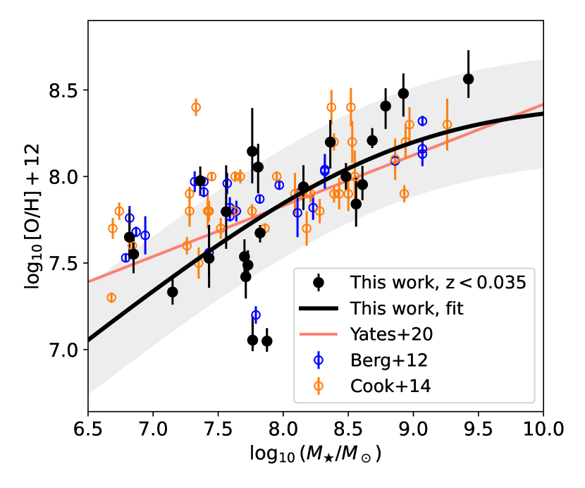
Figure 5: Stellar mass versus gas-phase metallicity for the galaxies in the reference sample ($z<0.035$) for which we are able to measure reliable auroral-line temperature metallicities. Our fit to the $0<z<0.035$ mass–metallicity relation is shown in grey, where the shaded region shows the $1\sigma$ intrinsic scatter of the fit. For context, we also show measurements of nearby galaxy samples using the same temperature-sensitive auroral line ratio approach that we apply here (Berg et al., 2012; Cook et al., 2014; Yates et al., 2020). All measurements are adjusted to a Kroupa (2001) IMF, but otherwise shown as published. We find good agreement between our sample and the literature.

Finally, in order to estimate the galaxies’ mass in oxygen we need an estimate of the total gas mass of the reference sample galaxies. We adopt individual H I masses for the reference galaxy samples and fit an average H I gas fraction as a parameter in our model. 28 of our reference galaxies have a match in the extragalactic ALFALFA catalog of Haynes et al. (2018); we estimate an H I mass for the remainder of the galaxies in our reference sample using the Bradford et al. (2015) relation. We find that the few galaxies that have an ALFALFA detection are in good agreement with the estimates from the Bradford et al. (2015) relation at their stellar mass. In Appendix D we take an alternate route to estimating $M_{g}$ by assuming a fixed star formation efficiency, and find that it does not affect the outcome of this analysis.

To arrive at an estimate for the total gas mass in our reference sample galaxies we will infer the average mass fraction of 21cm-bright H I as a free parameter in our model:

$$f_{21}{}=\frac{M_{\rm 21}}{M_{g}},$$ (14)

where $M_{g}$ is the total gas mass in hydrogen. This observationally defined quantity primarily traces the warm neutral medium (WNM), though there is evidence for significant emission from thermally unstable neutral hydrogen in the Solar Neighborhood. The total gas mass in the ISM, however, should include all phases of the ISM; if we assume that it is the warm neutral medium that is traced by 21 cm emission, we would expect a value of $f_{21}{}\approx 0.4$ for Solar Neighborhood-like conditions (Heiles & Troland, 2003).

4.4 Comparing Model Predictions to Observations

Finally, we must also include the effects of our selection function. This includes both the photometric selection described in Section 2.1, and the requirement for an emission line detection. We compute the expected $g-r$ color at luminosity distance $d_{L}(t_{i+1})$ and effective on-sky radius at angular diameter distance $d_{A}(t_{i+1})$ by computing reverse $k$-corrections directly from the spectra; we require that the galaxy have an apparent magnitude of $m_{r}<21$ to remain “observed”, which we will presently describe, at $t_{i+1}$. Galaxies that are flagged as observed at a given lookback time $t_{i+1}$ are excluded from our computation of the likelihood, which we will detail in the following section (Section 4.5).

The probability that any given galaxy will be securely redshifted by the SAGA survey is the product of the probability that the galaxy will be targeted, and the probability that the target will be sufficiently bright to obtain a secure redshift. Let us first consider the probability that a galaxy will be targeted.

The effective SAGA targeting scheme is based upon the apparent (galactic extinction-corrected) $r-$band magnitude of the galaxy, its effective $r-$band surface brightness, and its $g-r$ color (Mao et al., 2021). In order to quantify the probability that a retrogressed galaxy would have been selected for observation, we simply measure the fraction of galaxies that have observations from SDSS, GAMA, or SAGA AAT/MMT as a function of their (binned) photometric properties. This is done in three dimensions; for visualization purposes we show the projected targeted fraction for our photometric parameter space in Figure 6. In each panel group, the upper panels show the distribution of all possible targets (left, red) and the targeted galaxies (right, blue). The main panel shows the fraction of galaxies targeted as a function of their photometric properties, where the size of the box corresponds inversely to the uncertainty on the measured fraction assuming a binomial distribution. One can clearly see the imprint of the photometric selection described in Mao et al. (2021), wherein galaxies that are bluer and lower surface brightness are more likely to have been observed.

At each timestep, we compute the observed-frame $r$-band magnitude, $r$-band surface brightness, and $g-r$ color of each retrogressed galaxy. We compute the expected $g-r$ color at luminosity distance $d_{L}(t_{i+1})$ and the effective on-sky radius at angular diameter distance $d_{A}(t_{i+1})$ by computing reverse k-corrections directly from the spectra. We do not account for the change in the age and metallicity of the underlying stellar populations when computing this shift but note that the change in apparent magnitude due to the change in stellar mass and stellar age is small ($\Delta m_{r}\sim 0.1$) over our redshift range compared to the effect on the apparent magnitude from distance ($\Delta m_{r}\lesssim 7$).

At each timestep we estimate the targeted fraction by drawing from a uniform distribution bounded by the 95% confidence interval. We then sample from a uniform distribution bounded by zero and unity, and the galaxy is flagged as observed if the targeted probability exceeds the drawn number.

We then must consider whether the SAGA survey would be able to obtain a secure redshift for the galaxy at the proposed timestep. We estimate the H$\alpha$ detection limit as three times the standard deviation of the blank spectrum within $140(1+z_{i+1})$ Å of H$\alpha$ (we mask H$\alpha$, [N II]$\lambda$6548Å, and [N II]$\lambda$6583Å). To estimate the expected strength of H$\alpha$, we convert SFR$(t_{i+1})$ to an H$\alpha$ flux using the inverse of Equation 8, i.e.:

$$F_{\text{H$\alpha${}}}(t_{i+1})=\frac{\text{SFR}(t_{i+1})/[M_{\odot}\ \rm yr^{-1}]}{5.5\times 10^{-42}}\frac{1}{4\pi d_{L}^{2}(z_{i+1})}.$$ (15)

To be flagged as observable, we require that $F_{\text{H$\alpha${}}}(t_{i+1})$ exceed the $3\sigma$ detection limit defined above.

Figure 6: The effective photometric selection of the present sample. Each panel grouping shows the projected distribution of the targeting catalog (top left, red), the distribution of the present sample (top right, teal), and the fraction of galaxies for a given region of photometric parameter space that are in SAGAbg-A. In the main panel, the size of each box corresponds to the inverse of the uncertainty on the targeted fraction assuming a binomial distribution.

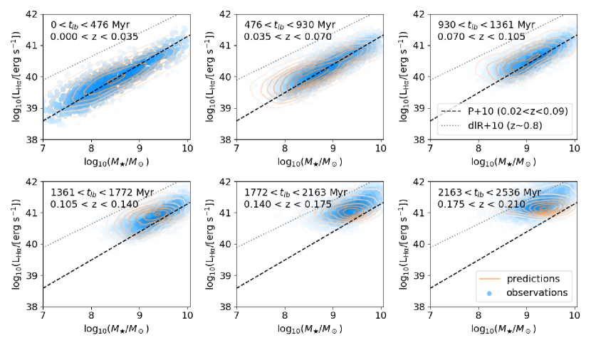
Figure 7: A comparison between the predicted (orange) and observed (blue) SAGA background sample as a function of redshift in the $M_{\star}$-$L_{\rm H\alpha}$ plane. Here we also show the SFMS fit of Peng et al. (2010) based off of SDSS ($0.02<z<0.09$) and that of de los Reyes et al. (2015) (the narrow-band NewH$\alpha$ survey, $z\sim 0.8$) to compare with established literature results.

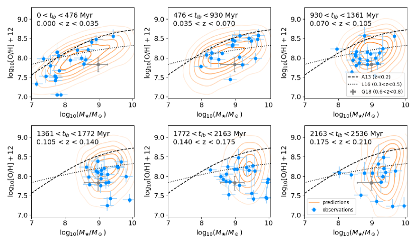
Figure 8: The same as Figure 7, but for the stellar mass-gas phase metallicity plane. Again we show literature results from other studies that derive metallicities from auroral oxygen lines: results from stacked SDSS spectra at $z<0.2$ (Andrews & Martini, 2013), from the MACT survey at $0.3<z<0.5$ (Ly et al., 2016), and at $0.6<z<0.85$ (Gao et al., 2018).

4.5 Parameter Estimation

With this model of the SAGAbg-A selection function in hand, we can now consider how to leverage this information during our inference of the physical parameters of interest

We first place a uniform prior on all three parameters of interest over a physically reasonable range, where the directly sampled parameter is $\log_{10}(\eta_{\rm m})$ rather than $\eta_{\rm m}$ itself.

$$\text{Pr}[a_{\rm SFH}{}] \propto\begin{cases}\text{const.}&\text{if\ }a_{\rm SFH}{}<4\\ 0&\text{else}\end{cases}$$ (16a)

$$\text{Pr}[\log_{10}\eta_{\rm m}] \propto\begin{cases}\text{const.}&\text{if\ }10^{-3}<\eta_{\rm m}{}<10^{3}\\ 0&\text{else}\\ \end{cases}$$ (16b)

$$\text{Pr}[f_{21}] \propto\begin{cases}\text{const.}&\text{if\ }0<f_{21}<1\\ 0&\text{else}.\\ \end{cases}$$ (16c)

Here we estimate our likelihood based on density estimation using a kernel density estimate over our model predictions for fixed parameter choice, sampling from the Bradford et al. (2015) $M_{\rm HI}-M_{\odot}$ relation and, for reference galaxies that do not have a secure direct temperature method metallicity estimate, our established reference mass–metallicity relation as shown in Figure 5.

As in the ISM property inference, we estimate the probability density functions independently and thus the joint likelihood can be written as:

$$\begin{split}\ln\mathcal{L}_{j}(\vec{\text{SFR}},\vec{M}_{\star},\vec{Z}_{O}|\vec{\theta}_{m},z_{j})&=\sum_{i}\mathcal{L}_{{{\color[rgb]{0,0,0}j}}}^{{{\color[rgb]{0,0,0}\rm SM}}}(\text{SFR}_{i},M_{\star,i}|\vec{\theta}_{m},z_{j})+\\ &\ \ \mathcal{L}_{{{\color[rgb]{0,0,0}j}}}^{\text{{{\color[rgb]{0,0,0}MM}}}}(Z_{O,i},M_{\star,i}|\vec{\theta}_{m},z{{\color[rgb]{0,0,0}{}_{j}}})\\ \ln\mathcal{L}(\vec{\text{SFR}},\vec{M}_{\star},\vec{Z}_{O}|\vec{\theta}_{m})&=\sum_{j}\ln\mathcal{L}_{j}(\vec{\text{SFR}},\vec{M}_{\star},\vec{Z}_{O}|\vec{\theta}_{m},z_{j}),\end{split}$$ (17)

where $X_{i}$ indicates the $i^{\text{th}}$ observation of quantity $X$ (SFR, stellar mass, or gas-phase metallicity) in a given redshift bin, $z_{j}$ is the $j^{\text{th}}$ redshift bin, and $\vec{\theta}_{m}$ are the model parameters ($a_{\rm SFH}{}$, $\eta_{\rm m}{}$, and $f_{21}{}$) adopted at walker step $m$. $\mathcal{L}_{j}^{\rm MM}$ and $\mathcal{L}_{j}^{\rm SM}$ refer to the likelihood of the data in metallicity-stellar mass space and SFR-stellar mass space, respectively. We estimate the likelihood of the higher redshift ($z>0.035$) samples via a Gaussian kernel density estimate with bandwidth $N^{-1/(d+4)}$ (i.e. Scott’s Rule, Scott 1992) computed from the predictions of our model, where we redraw from the $M_{\star}-M_{21}$ and $M_{\star}-Z_{O}$ relations ten times for each density estimate of the predictions. In order to incorporate our knowledge of our sample selection function, we exclude retrogressed galaxies whose properties lie outside of the SAGAbg-A selection/detection criteria as described in Section 4.2 when constructing the density estimate.

This kernel density estimate allows us to arrive at a non-parametric form for both $\mathcal{L}^{\text{SM}}_{j}(\text{SFR}_{i},M_{\star,i}|\vec{\theta}_{m},z_{j})$ and $\mathcal{L}^{\text{MM}}_{j}(Z_{O,i},M_{\star,i}|\vec{\theta}_{m},z_{j})$. We then compute the likelihood of observing the sample at the $j$^th redshift bin for all galaxies in the SAGAbg-A sample at the relevant redshifts. In the case of the star-forming main sequence, we compute the likelihood over all galaxies in the sample. In the case of the mass-metallicity relation, we compute the likelihood over only the galaxies that have a measured oxygen abundance from the auroral lines discussed in Section 3.2. We note that, as discussed in Appendix C, our estimate of the mass-loading factor would not be significantly affected if we were to use a strong-line indicator of metallicity that agrees with our low redshift ($z<0.035$) measure of the mass-metallicity relation.

As above, we use the emcee implementation of the Affine Invariant Markov Chain Monte Carlo ensemble sampler (Foreman-Mackey et al., 2013) for parameter inference. We run the chain for 10000 steps with 32 walkers and visually confirm chain convergence.

5 Results

5.1 The SAGAbg-A Sample in $M_{\star}$-SFR Space

Here we discuss the observed evolution of the SAGAbg-A sample in stellar mass and star formation rate in both our observations and model. The observed evolution is a product of both the physical evolution and the effect of our observational limitations and selection on the $M_{\star}-L_{H\alpha}$ plane as a function of redshift. Becuse the SAGAbg-A sample contains only star-forming galaxies (due to our emission line detection requirements), we will compare our results in this section to literature measures of the star-forming main sequence (SFMS).

Each panel in Figure 7 shows a redshift slice of $\Delta z=0.035$ ($370<\Delta t_{lb}<480$ Myr) with our observed sample shown by the blue points (colored by a Gaussian kernel density estimate to visually indicate density) and our model predictions shown by orange contours. In each panel, we also show the SDSS SFMS ($0.02<z<0.09$) of Peng et al. (2010) as a dashed black line and the NewH$\alpha$ SFMS ($z\sim 0.8$) of de los Reyes et al. (2015) as a dotted black line; these two surveys are chosen due to their redshift range and use of H$\alpha$ as a SFR indicator.

We find good agreement between our observations and model predictions both visually in Figure 7 and through a quantitative comparison of summary statistics in Appendix E. This supports our choice of a simple, linear approximation to the recent SFH of the galaxies in our sample (see Equation 10). The average star formation rate at fixed stellar mass in our sample moves upwards by around 0.4 dex across our sampled redshift range, varying smoothly between the relations of Peng et al. (2010) and de los Reyes et al. (2015). The shift of the SFMS shown in Figure 7, as stated above, is a combination of a physical shift in the SFMS and an observational shift imposed by the H$\alpha$ flux limit of our spectra. In Paper II of this series, we will examine the implications of the physical component of this shift.

5.2 The Mass–Metallicity Relation

Having now established that our simple retrogression model reproduces our observed sample in the stellar mass-star formation rate plane, we will now consider the results of the somewhat more complex stellar mass-gas phase metallicity (MZR) plane.

In Figure 8 we show the MZR analog of Figure 7, wherein each panel shows our observed auroral line galaxies in blue and model predictions in orange. In each panel, we also show literature measurements that use the same metallicity method and bound our redshift limits. Given the systematic uncertainties that underpin strong line metallicity calibrations (for a recent review, see Kewley et al., 2019) and the importance of comparing equivalent measures in matters of redshift evolution, we only compare to literature measurements of metallicity that have been made with the auroral lines that we consider in this work. We show mass–metallicity relations derived from stacked SDSS spectra by Andrews & Martini (2013) at $0<z<0.2$, individual galaxy measurements at $0.3<z<0.5$ by Ly et al. (2016), and individual galaxies at $1.5<z<3.5$ from the MOSDEF survey by Sanders et al. (2020). We convert all relations to a Kroupa IMF from a Chabrier (2003) IMF. At $z<0.035$ our measurements agree well with Andrews & Martini (2013), while at $0.17<z<0.21$ our measurements are in good agreement with Ly et al. (2016).

Similar to the star-forming main sequence, there is good agreement between our observations, model predictions, and literature results. As with the SFMS, we evaluate the success of our model based on the evolution of summary statistics in Appendix E, though visual concordance is also shown in Figure 8.

Previous works have found evidence for an anti-correlation between star formation rate and gas-phase metallicity at fixed stellar mass (Mannucci et al., 2010; Andrews & Martini, 2013), though the strength of this effect and its dependence on the method of metallicity estimation is still disputed (Hughes et al., 2013; Sánchez et al., 2013; Telford et al., 2016). Our star formation rate sensitivity limit increases with redshift due to distance. To test whether the observed change in the mass–metallicity relation can be entirely attributed to a correlation between SFR and gas-phase metallicity, we consider the galaxies in our sample with star formation rates exceeding the minimum star formation rate observed in our sample of [O III]$\lambda$4363Å-detected galaxies at $z>0.17$ (our highest redshift bin). That is, we consider only the galaxies that should have emission lines that are detectable at a distance corresponding to $z=0.17$, all other properties of the galaxy being held constant. We find an anti-correlation between redshift and gas-phase metallicity with a best-fit slope of $d(\log_{10}[\text{O/H}])/dz=-1.7^{+0.9}_{-0.7}$, which is consistent with the slope of the Taylor expansion of the Ly et al. (2016) relation of $d(\log_{10}[\text{O/H}])/dz=-1.0^{+0.2}_{-0.1}$ when measured over $0<z<1$.

Despite using auroral lines to derive oxygen abundances, it is not entirely straightforward to compare our results with that of Andrews & Martini (2013). They directly stacked SDSS spectra to measure auroral line metallicities, and the ratio of the mean of the emission line need not necessarily be the mean of the emission line ratios (which itself need not reflect the mean of the $T_{e}$ distribution!); nevertheless, it is encouraging to see the agreement with the stacked SDSS results and the present work at $0<z<0.035$.

It is crucial to remember that all of these works (the present sample included) are subject to emission line strength biases in that the strong line emitters tend to be the galaxies where weak auroral line metallicity measurements may be made. However, the overall body of literature indicates that understanding both observational results and observational limitations will be crucial in understanding the history of low-mass galaxy enrichment.

Figure 9: Posterior distributions of our modeled parameters $a_{\rm SFH}{}$, $\eta_{\rm m}{}$, and $f_{21}{}$. The posterior distributions shown here are smoothed by a Gaussian kernel of $\sigma=1.5$.

5.3 Model Fits: $\eta_{\rm m}{}$ (and $a_{\rm SFH}{}$, $f_{21}{}$)

Having now demonstrated that our model is able to reproduce the observed SAGAbg-A sample distribution in $M_{\star}$-SFR-$Z_{O}$-$z$ space, let us consider the inferred parameters themselves. As laid out in Section 4, we fit three parameters in this model: $a_{\rm SFH}{}$, which parameterizes the average increase in SFR as a function of redshift (Equation 10), $\eta_{\rm m}{}$, the mass-loading factor (Equation 12), and $f_{21}{}$, the average 21cm-bright H I mass fraction (Equation 14). In Figure 9 we show a corner plot of the inferred parameters $a_{\rm SFH}{}$, $\eta_{\rm m}{}$, and $f_{21}{}$. There is no evidence for strong correlations in the joint posteriors of our parameter inference, and we report the median and 68% scatter in Figure 9.

Taking the inferred parameters in turn, let us first consider the recent evolution in the average SFH of the sample. We find evidence for a moderate increase in SFR as a function of lookback time, indicating that the shift in the observed SFMS cannot be fully explained by our observational limits, and is due in part to a physical shift upwards in the star-forming main sequence from $t_{lb}$$\sim 0$ to $t_{lb}$$\sim$2.5 Gyr. This effect will be more thoroughly examined in the second paper of this series (Kado-Fong et al., in preparation).

Finally, we arrive at an estimated mass-loading factor of $\eta_{\rm m}{}=0.92^{+1.76}_{-0.74}$. This inferred value for the mass-loading factor is close to unity (i.e., one solar mass of gas expelled per year for each solar mass of stars formed), and was derived using a framework that differs significantly from direct measures of the mass-loading factor. In the following discussion, we will consider the implications of this relatively low mass-loading factor in the broader context of previous observational measures of $\eta_{\rm m}{}$ and current theoretical predictions for mass-loading in low-mass galaxies.

Because $\eta_{\rm m}{}$ could be a mass-dependent quantity, it is also important to constrain the stellar mass range over which this $\eta_{\rm m}{}$ inference is sensitive. To do so, we rerun our inference while varying both the upper and lower limits on stellar mass until the uncertainty on any of the inferred parameters exceeds twice that of the uncertainty in the fiducial run. The effective stellar mass range of the sample as characterized by this empirical method is $10^{7.5}\lesssim M_{\star}/M_{\odot}\lesssim 10^{9.5}$. This range also corresponds roughly to the 10^th and 90^th percentiles of the stellar mass distribution of the reference sample.

6 Discussion

We now consider the implications of our estimated mass-loading factor on the contemporary landscape of measurements and predictions of the mass-loading factor. This section begins with a comparison between our inferred $\eta_{\rm m}{}$ and observational results from the literature that are based on direct measurements of mass outflow rates (Section 6.1). We then compare to contemporary results from models and simulations of low-mass galaxies in Section 6.2 before touching on the limitations of our simple model for the low-mass galaxy population in Section 6.3.

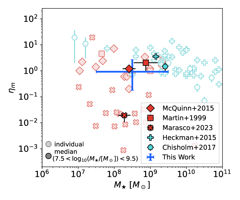
Figure 10: Mass loading factor vs. stellar mass, comparing our results to direct observations of outflowing gas. These studies either rely on detection of outflowing gas in H$\alpha$ emission (red circles show McQuinn et al. 2019, red squares show Martin 1999; red line shows Marasco et al. 2023) or from UV absorption features (aqua crosses show Heckman et al. 2015; aqua circles show Chisholm et al. 2017). For each study, we show both the individual galaxy measurements as light points and the median of the sample in the stellar mass range $7.5<\log_{10}(M_{\star}/[M_{\odot}])<9.5$ as the dark points with black outlines. The uncertainties on the median of the literature samples are estimated via bootstrap resampling.

6.1 Comparison to Direct Measures of $\eta_{\rm m}{}$

There are two main methods of measuring $\eta_{\rm m}{}$: direct and indirect. Direct measures of $\eta_{\rm m}{}$ are typically made for individual galaxies by tracing gas that has been deemed to be outflowing by some definition, while indirect measures trace the impact that outflows enact on some other aspect of galaxy evolution at a sample or population level. The study at hand is a type of indirect observation, albeit one done in a differential manner.

Our value of $\eta_{\rm m}{}$ is in good agreement with most direct measurements of galaxies in the relevant stellar mass range. In Figure 10, the marker shape indicates the individual study while the color represents the type of measurement: red points indicate direct measurements via H$\alpha$ emission, while turquoise points indicate direct measurements via UV absorption.

We find good agreement between our results and those of McQuinn et al. (2019) and Martin (1999), both of whom use H$\alpha$ emission to identify and measure mass outflow rates. The spectroscopic study of Marasco et al. (2023) find a near-negligible mass-loading factor of $\eta_{\rm m}{}\approx 0.02$ for low-mass galaxies based off of an analysis of the flux-weighted velocity distribution of H$\alpha$ lines in integral field unit (IFU) spectroscopy. A discrepancy between the literature results may be related to a difference in methodology; whereas the first two studies identify H$\alpha$ emitting gas that is spatially offset from host dwarf galaxies (Martin, 1998, 1999; McQuinn et al., 2019), Marasco et al. (2023) decompose the full H$\alpha$ line profile of the galaxy of face-on galaxies into outflowing and non-outflowing components.

A mass-loading estimate based on H$\alpha$ should trace only $\eta_{\rm m}{}$ of gas in the warm phase, whereas the present work does not distinguish between ISM phases. The concordance is not surprising, however, if we consider that the warm phase is predicted to dominate mass outflow (Kim et al., 2020; Steinwandel et al., 2022b). An estimate of $\eta_{\rm m}{}$ as defined by Equation 12 could therefore be reasonably expected to be in agreement with measures of $\eta_{\rm m,warm}$, the mass-loading factor in the warm (ionized) phase.

We derive an estimate for the mass-loading factor that is somewhat lower than the estimates that have been made from UV absorption features. In the overlapping region of stellar mass space, we find good agreement with Chisholm et al. (2017), though we caution that this includes only two galaxies from their sample. The Heckman et al. (2015) median mass-loading factor, $\eta_{\rm m}\approx 2.5$, is slightly higher than our estimate. Both UV-based studies shown here have a high fraction of starbursting dwarfs; a change in $\eta_{\rm m}{}$ as a function of SFR or $\Sigma_{\rm SFR}$ is another plausible explanation for the offset in $\eta_{\rm m}{}$ given the spatially coherent nature of star formation and star formation-driven outflows.

We note that is also not straightforward to compare H$\alpha$ and UV-based studies against each other. First, the H$\alpha$ literature studies and this work use H$\alpha$-derived SFRs, which probe $\sim 5$ Myr timescales, while UV-based star formation rates probe significantly longer ($\sim 100$ Myr) timescales. Our own indirect estimate of $\eta_{\rm m}{}$ is averaged over $\sim 400$ Myr given the size of our redshift bins. Thus, we may expect our estimate of $\eta_{\rm m}{}$ to be biased low compared to direct measurements if the majority of the outflowing mass recycles on timescales short compared to 400 Myr. In practice, the concordance between our results and the direct measurements presented here implies that this effect does not strongly impact the comparison. Indeed, the study most significantly offset from our results and other literature results (Marasco et al., 2023) estimates mass-loading factors significantly lower than our own estimate.

The concordance between the mass-loading factor we present here and the results from direct detection studies is encouraging because these methods to estimate $\eta_{\rm m}{}$ demand different simplifying assumptions. Directly measuring outflow rates requires strong assumptions about the geometry and velocity of the outflows, while our differential method requires strong assumptions about ISM mixing and accretion timescales. There is minimal overlap between the assumptions made by direct outflow measures and our indirect differential approach: arriving at the same answer is an important measure of observational consensus-building in an arena where theoretical models differ by orders of magnitude.

Figure 11: Mass loading factor vs. stellar mass, comparing our results to models that infer $\eta_{\rm m}{}$ as a parameter influencing some other property of the galaxy population. We show the gas regulator model of Lilly et al. (2013) as a solid green line, the fit to the mass–metallicity relation of Lin & Zu (2023) as a dashed purple curve, and the model of the total oxygen galaxy budget of Zahid et al. (2012) as an orange shaded region.

6.1.1 Comparison to $\eta_{\rm m}{}$ Inferred from Analytic Models

We compare our results to three indirect constraints on the mass-loading factor in low-mass galaxies: two studies that inferred $\eta_{\rm m}{}$ from the $z\sim 0$ mass–metallicity relation (Lilly et al. (2013) and Lin & Zu (2023)), one that compared the mass–metallicity relation between surveys at different redshifts (Zahid et al., 2012), and one that inferred $\eta_{\rm m}{}$ from the stellar-to-halo mass and ISM-to-stellar mass relations (Carr et al., 2022).

Our estimate of $\eta_{\rm m}{}$ is in good agreement with the gas regulator model of Lilly et al. (2013) at the high mass end of our sample and significantly lower than the chemical evolution model estimate of Lin & Zu (2023), despite the fact that both studies aim to reproduce the observed SDSS $M_{\star}$-metallicity-SFR distribution at $z\sim 0$ to estimate $\eta_{\rm m}{}$. We also find good agreement with the inter-survey comparison of SDSS and DEEP2 by Zahid et al. (2012). All three of these studies use gas-phase metallicities estimated through strong-line calibrations — Lilly et al. (2013) and Lin & Zu (2023) moreover use the same SDSS metallicities as measured by Mannucci et al. (2010). These calibrations are known to incur systematic uncertainties of up to $\sim\!1\text{ dex}$ both between different line ratio estimators (Kewley & Ellison, 2008) and between different calibrations of the same line ratio estimators (Kewley et al., 2019). A systematic offset in metallicity could explain a difference between our results and those of Lin & Zu (2023), but not the difference between the results of Lin & Zu (2023) and Lilly et al. (2013).

We also find good agreement with Carr et al. (2022) in that they argue for winds with a low mass-loading factor ($0.1\lesssim\eta_{\rm m}{}\lesssim 10$) and a high energy loading factor. However, we note that the form of their mass-loading factor dependence with halo mass was chosen to agree with direct measurements of $\eta_{\rm m}{}$, and thus is not independent of the concordance that we find with direct observations of $\eta_{\rm m}{}$.

6.2 Comparison to Theoretical Predictions

In Figure 12 we compare to predictions of $\eta_{\rm m}{}$ from the simulation literature. Simulations provide a more direct view of the mass-loading factor, as outflowing gas can be explicitly traced and tabulated. However, the exact definition of outflowing gas varies significantly from work to work: a prediction for the mass-loading factor is typically set by computing mass flux for some subset of the gas classified as outflowing through a slab or shell displaced a few kpc from the galaxy of interest. Outflows are either selected to be all gas that is moving away from the midplane ($v_{z}>0$ or $v_{R}>0$, depending on the coordinate system used, see e.g. Muratov et al., 2015; Kim & Ostriker, 2018; Hu, 2019; Nelson et al., 2019; Steinwandel et al., 2022a, b) or a subset of the gas that is predicted to escape to a given midplane distance (Anglés-Alcázar et al., 2017; Pandya et al., 2021). Both the height and outflow selection criteria can change the estimate of $\eta_{\rm m}{}$ by a factor of several (Nelson et al., 2019; Pandya et al., 2021); we will discuss the effect of these choices on our approach to simulation comparison below.

To illustrate the implications of where and how simulators measure their mass-loading factors, in Figure 12 we show with outlined points only those mass-loading factor predictions for a set of works in which the mass outflow rate is computed with a velocity cut of $v_{\rm out}>0$. The differences between the predictions here should be roughly indicative of the differences in physical prescriptions and numerical effects for these simulations. In the same color, we also show an expanded view of the theoretical landscape which includes a wider range of methods to determine $\dot{M}_{\rm out}$. It is generally understood that differences in subgrid models for star formation – and in particular supernova – feedback as well as numerical methods for how energy and momentum from star formation feedback contribute significantly to the range of mass-loading factors seen in simulations. Furthermore, here we see that $\eta_{\rm m}$ can vary by a factor of several for the same simulation; Pandya et al. (2021) showed in particular that mass-loading factors derived from the FIRE simulations can vary between $\eta_{\rm m}\sim 5$ and $\eta_{\rm m}\sim 30$ for galaxies at $\log_{10}(M_{\star}/M_{\odot})$$\approx 8.5$ due only to differences in how outflows are identified.

6.2.1 Comparison to High Resolution Galaxy Simulations

We consider two resolved-ISM, non-cosmological galaxy simulations close to our mass range: the LMC-mass galaxy simulation of Steinwandel et al. (2022b), with a gas mass resolution of $m_{\rm gas}=4M_{\odot}$, and the lower mass ($M_{\star}\approx 2\times 10^{7}M_{\star}$) simulation of Hu (2019), with a mass resolution of $m_{\rm gas}=1M_{\odot}$. We find that these two simulations, which bound the stellar mass range we probe, also bound our prediction for $\eta_{\rm m}{}$.

Let us first compare to the Steinwandel et al. (2022b) of the LMC-mass galaxy. We show the time-averaged estimate of $\eta_{\rm m}{}$ at $z=\{3,5,10\}$ kpc from the disk (where 10 kpc is approximately 0.1 $R_{vir}$). There is relatively little change in $\eta_{\rm m}{}$ as a function of height off the midplane beyond $z\sim 1$ kpc relative to the range of $\eta_{\rm m}{}$ proposed by the full set of simulations we consider. We also compare to the lower mass simulation of Hu (2019) using their asymptotic value of $\eta_{\rm m}{}(R)$. The mass-loading factor estimated by Hu (2019) is somewhat higher than our estimated $\eta_{\rm m}{}$. This could be consistent with the picture of a stellar mass-dependent $\eta_{\rm m}{}$, but as we discussed in Section 6.1, it remains unclear how strong this mass dependence is in observations.

Figure 12: A comparison between our results (the blue error bar in each panel) to various theoretical predictions from the literature. The color denotes the class of simulation, while the shape of the marker denotes the individual study as described in the text. Individual galaxy simulations are shown in green (the green triangle shows Hu 2019; the green circles show Steinwandel et al. 2022a and Steinwandel et al. 2022b), the FIRE zoom simulations in orange (the solid orange line shows Muratov et al. 2015; the dotted orange line shows Anglés-Alcázar et al. 2017; the dashed orange line shows Pandya et al. 2021) and mauve shows results from Illustris TNG50 (Nelson et al., 2019) where outflows are defined as $v_{r}>0$ (upper curve) and where outflows are defined as $v_{r}>150\ {\rm km\ s^{-1}}{}$ (lower curve). All literature references where outflows are defined with a $v_{z}>0$ cut at some midplane distance are shown by outlined markers.

6.2.2 Comparison to Cosmological Simulations

Finally, we consider the big box and zoom cosmological simulations. All three orange lines in Figure 12 originate from analyses of the FIRE-1 and FIRE-2 simulations (Muratov et al., 2015; Anglés-Alcázar et al., 2017; Pandya et al., 2021), with baryonic mass resolutions of $250\leq m_{\rm bary}\leq 7100M_{\odot}$. As demonstrated in Pandya et al. (2021), the difference in the three FIRE $\eta_{\rm m}{}$ estimates originates from a difference in how $\dot{M}_{\rm out}$ is defined, rather than a difference in physical prescriptions between FIRE-1 and FIRE-2. In particular, Muratov et al. (2015) uses a $v_{r}>0$ cut at $R=0.25R_{\rm vir}$ (similar to the isolated galaxy simulations), Anglés-Alcázar et al. (2017) directly tracks the displacement of gas out of the galactic midplane, and Pandya et al. (2021) leverages a cut on the Bernoulli velocity at $0.1-0.2R_{\rm vir}$ to distinguish between escaping winds and gas that may remain bound at large radii.

Having laid out the guides by which these three works compute $\eta_{\rm m}{}$, it is likely that a true comparison to our $\eta_{\rm m}{}$ estimate would be somewhere between that of Muratov et al. (2015) and Pandya et al. (2021). The mass-loading estimate of Anglés-Alcázar et al. (2017) likely includes gas that is quickly recycled into the ISM and would therefore be systematically higher than our $\eta_{\rm m}{}$ estimate as a matter of definition. On the other hand, the mass-loading factor estimate of Pandya et al. (2021) could be systematically offset to lower $\eta_{\rm m}{}$ than our estimate because their definition attempts to only capture gas that will truly escape the galaxy, excluding gas that may remain bound at large radii. Because that bound gas would remain unavailable for future generations of star formation (for some timescale that is long compared to our sample redshift range), it should be included in our estimate of $\eta_{\rm m}{}$. The positive radial velocity at $0.25R_{\rm vir}$ criterion that Muratov et al. (2015) make to define $\eta_{\rm m}{}$ is also closely aligned to that of Steinwandel et al. (2022b).

We additionally note that low-mass FIRE galaxies have been found to have low H I-to-stellar mass ratios compared to observed galaxies (El-Badry et al., 2018; Kado-Fong et al., 2022b); this finding is in agreement with a picture in which the FIRE-1 and FIRE-2 mass-loading factors are systematically displacing more gas from low-mass halos than proceeds in the observed Universe, though it is certainly not the only explanation for such a discrepancy.

Few big box cosmological simulations have a sufficient mass resolution to interpret the implication of mass-loading on low-mass halos, and even fewer have reported mass-loading factors. With a baryonic mass resolution of $m_{\rm bary}=8\times 10^{4}M_{\odot}$, Illustris TNG50 (Nelson et al., 2019) is the highest resolution and smallest box size run of the TNG suite and has published mass-loading factors, though these mass-loading factor predictions were computed at $z=2$. It is unclear how the mass-loading factor is expected to evolve between $z=2$ and $z=0$, though some simulations have reported negligible evolution (Pandya et al., 2021). We show the TNG50 results as thick mauve curves: the upper curve shows $\eta_{\rm m}{}$ at $R=10$ kpc where outflows are defined by $v_{r}>0$, and the lower curve shows the same where outflows are defined as $v_{r}>150~{}{\rm km\ s^{-1}}{}$. In both cases the resulting $\eta_{\rm m}{}$ is higher than our estimate by around an order of magnitude.

6.3 Limitations and Possible Biases

As we emphasized earlier in this text, the model presented in this work is by design a narrow and incomplete view of galaxy evolution — our present scope is not to instantiate the galaxy population from first (or some facsimile for first) principles but to explain the evolution over a small range of physically interesting parameter space.

In order to reconcile our results with the mass-loading factors produced in cosmological simulations, we would need to be significantly underestimating the mass-loading factor. In our fiducial equilibrium model (Equation 12), the derivative of $\dot{Z}_{O}$ (the time derivative of the oxygen abundance) with respect to the mass-loading factor can be written as

$$\begin{split}\frac{d\dot{Z}_{O}}{d\eta_{\rm m}}(t)=-\frac{Z_{O}(t)y_{z}\dot{M}_{\star}(t)}{M_{g}}.\end{split}$$ (18)

If we assume that $\dot{Z}_{O}$ is non-negative, an increase in the mass-loading factor results in a lower value of $|\dot{Z}_{O}(t)|$; that is, a shallower evolution in the mass–metallicity relation. If the true mass-loading factor were higher, as cosmological simulations require, we would need to be incomplete in low-metallicity galaxies at low redshift and/or incomplete in high-metallicity galaxies at high redshift, particularly at the high mass end. We find it unlikely that we are incomplete at low metallicity at low redshift given the concordance of our low-redshift mass–metallicity relation with that of deeper nearby galaxy samples (as shown in Figure 5). Though higher metallicity objects tend to have weaker [O III]$\lambda$4363Å lines with respect to the brighter O III emission lines, potentially imposing a bias at high redshift, the concordance that we reach between strong line and auroral line indicators (see Appendix C) that it is unlikely that the discrepancy between our estimate and theoretical requirements can be explained by observational incompleteness.

We note that our emission line-based selection produces a sample that contains relatively fewer satellite galaxies with respect to the overall satellite fraction expected at our stellar mass range (see Appendix G for details on our estimated satellite fractions). The mass-loading factors calculated from the high-resolution, non-cosmological simulations are based on completely isolated galaxies, while the mass-loading factors for the cosmological simulations include satellite galaxies. If our concordance with the resolved-ISM simulations were due to the impact of environment rather than star formation feedback prescriptions, the lowest-SFR galaxies that are missing from our sample – at this mass range, the transitional satellites – would need to have tremendously high mass-loading factors. We consider this situation unlikely: empirical studies have suggested that $\eta_{\rm m}$ is either insensitive to or increases with SFR (as discussed in Section 6.1).

Finally, it is also worth considering that the subset of galaxies at a given redshift for which we are able to measure electron temperatures via auroral lines is biased towards those galaxies with the highest star formation rates, as these galaxies tend to have higher overall emission line fluxes. There is evidence that there is a relationship between the star formation rate, stellar mass, and gas-phase metallicity of galaxies, called the Fundamental Metallicity Relation (FMR, Mannucci et al., 2010; Andrews & Martini, 2013). However, there has been significant discussion in the literature as to the strength, systematics, and even the very existence of this relation (Hughes et al., 2013; Sánchez et al., 2013; Telford et al., 2016; Pistis et al., 2023). Nevertheless, if we consider the effect that the FMR-as-observed would have on our sample, we may expect our local mass–metallicity relation to be biased low due to our need to detect the weak auroral lines to estimate a metallicity and the stated anti-correlation between gas-phase metallicity and star formation rate. However, we note that as shown in Appendix C, we reach the same estimate of the mass-loading factor for most choices of strong line calibrators.

By model design, incurring a systematic offset in gas-phase metallicity at fixed stellar mass in our reference sample will be partially accounted for by an offset in the same direction across the full sample. Furthermore, and quite apart from the model construction, our observed mass–metallicity relation is in good agreement with literature relations at both $z\sim 0$ (Berg et al., 2012; Andrews & Martini, 2013; Cook et al., 2014) and with the measured rate at which the mass–metallicity relation evolves (Ly et al., 2016). Though these studies may also be subject to the same potential SFR–metallicity biases, the heterogeneity of depth of the datasets — which directly controls the lowest H$\alpha$ luminosity, and thus SFR, that is included at a given distance — makes it difficult for such a concordance to be reached if the impact of a fundamental metallicity relation strongly biased the resulting observed MZR. We conclude that the discrepancy between our measured mass-loading factor and those required by cosmological simulations is unlikely to be a result of a systematic bias in our method.

7 Conclusions

In this work, we have used the background (non-SAGA host satellite) spectra collected by the SAGA survey to probe the star-forming cycle of low-mass galaxies in the $z<0.21$ Universe. The SAGA survey’s limiting magnitude is around a magnitude deeper than past wide-field efforts ($m_{\rm lim,SAGA}=20.75$), making the SAGAbg-A galaxies a novel window into the low-mass and low-redshift Universe.

In this work, we examined the apparent evolution of the star-forming main sequence and the stellar mass-gas phase metallicity relation within the last $\sim$2.5 Gyr as a method to constrain the star formation cycle at low redshift. We constructed a simple “retrogression” model to trace the evolution of our sample as a function of redshift. In essence, rather than attempt to instantiate the galaxy sample from theoretical principles, we ask whether we can accurately predict the appearance of the sample in $M_{\star}-\text{SFR}-Z_{\text{O}}$ space as a function of redshift by evolving our lowest redshift sample backward in time. At each timestep, we: remove the mass in stars that were made during the redshift bin (equivalently $\Delta t$) given the galaxy’s SFR, remove the yield in oxygen that was generated by those stars, and restore to the ISM both the mass that had been locked in those stars and the gas that had been expelled by star formation feedback as quantified by some value of the mass-loading factor, $\eta_{\rm m}{}\equiv\dot{M}_{\rm out}/\text{SFR}$.

In the main technical thrust of this work, we showed that:

• Our model, which includes both the physical evolution of the SAGAbg-A sample and the sample observability as imposed by the SAGA selection and detection criteria, can successfully predict the apparent redshift evolution of the sample in stellar $M_{\star}$-$Z_{O}$-SFR space (see Section 5.1 and Section 5.2).

• Our best-fit model favors a positive evolution of the SFMS normalization (which will be presented in greater depth in Paper II) and a low, near-unity mass-loading factor at $\eta_{\rm m}{}=0.92^{+1.76}_{-0.74}$ (Section 5.3).

The uncertainty on our estimate of the mass-loading factor is dominated by the relatively small number of galaxies for which we can measure a “direct” auroral line gas-phase metallicity. A large increase in the number of low-mass galaxies at appreciable redshift (i.e. $z\gtrsim 0.03$) for which these weak auroral lines are confidently detected would allow a stellar mass dependence to be introduced into this model.

In the context of the mass-loading literature, we found that:

• Our estimate of $\eta_{\rm m}{}$ is consistent with recent observational results from studies that directly estimate the mass outflow rate from detections of extra-planar gas (Section 6.1).

• Our measure of $\eta_{\rm m}{}$ is in good agreement with some, but not all, estimates of the mass-loading factor made by modeling the mass-metallicity relation or other aspects of galaxy chemical evolution (Section 6.1.1)

• We find good agreement with $\eta_{\rm m}{}$ measurements of single galaxy simulations (Section 6.2.1). However, our estimate of $\eta_{\rm m}{}$ is significantly lower than cosmological zooms and big box simulations, which predict mass-loading factors of up to $\eta_{\rm m}\approx 50$ over our stellar mass range (Section 6.2.2).

The fact that we arrive at consistent values of the mass-loading factors compared to direct measurements despite approaching the $\eta_{\rm m}{}$ measurement problem with a very different set of assumptions — our retrogression model makes strong assumptions about short-term galaxy evolution and ISM mixing, while direct $\eta_{\rm m}{}$ studies make strong assumptions about the geometry and kinematic structure of the outflows — is a crucial step forward for consensus-building in a volume of parameter space where theoretical predictions differ by more than an order of magnitude.

Our results join a growing body of both observational and theoretical work that indicate that low-mass galaxies are not as efficient at moving gas to large radii as has been claimed is required in some simulations to produce realistic galaxies in this mass range. Due to the importance of star formation and star formation feedback in low-mass galaxies, changing the efficiency at which outflows are launched would not only have implications for the chemical enrichment of dwarfs, but also for their stellar structure (El-Badry et al., 2016; Kado-Fong et al., 2020b, 2022b), gas content (El-Badry et al., 2018; Mancera Piña et al., 2019; Pandya et al., 2020), and structural diversity (Mancera Piña et al., 2020; Kado-Fong et al., 2021; Cardona-Barrero et al., 2023).

This paper represents a first effort using the SAGA background spectra, but the range of low-mass galaxy science that can be done is far from exhausted in this work. In Paper II of this series, we will extend the model presented here to consider the physical evolution of the low-mass star-forming main sequence and the implications of that evolution for constraints of galaxy evolution models at low redshift. The line measurements and abundance inferences will also be released as part of a future SAGA data release (Mao et al., in preparation) such that the information presented in this work will be accessible to the broader astronomical community.

Appendix A Flux Calibration and Line Measurement of the Spectra

To ensure that we achieve reasonable line fits, we test our flux recovery for a sample of galaxy spectra with reliable spectroscopic redshifts (nQ$>2$ in the GAMA DR4 StellarMassesLambdarv20 catalog) from the GAMA survey at $0<z<0.5$ with $M_{r}>-10$. We only consider the flux-calibrated spectra in the DR4 release (i.e. those originating either from GAMA or SDSS). Both our measurements and the GAMA DR4 catalog (GaussFitComplexv05) should be corrected for stellar absorption, but not for reddening.

In Figure 13 we show a comparison between the GAMA catalog H$\alpha$ flux measurements and our analogous flux measurements. We find an overall excellent agreement, though there is a tail wherein our measured flux is lower than the GAMA catalog values (i.e. below the 1:1 line in Figure 13). This may be due to differences in how H$\alpha$ absorption is handled, as H$\alpha$ absorption is not typically resolved in AAT/2dF spectra for these galaxies.

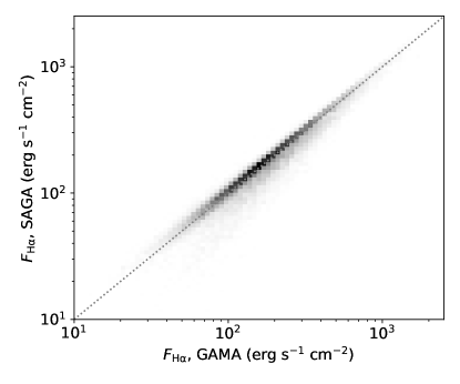
Figure 13: A comparison between our measured H$\alpha$ fluxes and GAMA DR4 catalog fluxes for GAMA galaxies in our stellar mass and redshift range. Both measures are nominally corrected for stellar absorption, but not for dust. We show here only galaxies with an H$\alpha$ SNR greater than 3 with a positive H$\alpha$ flux error in the GAMA DR4 catalog.

We additionally test that our spectra flux calibration is accurate by comparing to SAGAbg-A targets for which both SAGA AAT/2dF/MMT/Hectospec and GAMA DR4 spectra were obtained. In Figure 14 we compare absorption-corrected H$\alpha$ fluxes from this overlap, discarding galaxies where $A_{\lambda}(H\alpha)>3$ or $L_{H\alpha}<L_{H\alpha,\lim}$ in our SAGA spectra measurements. We find a good agreement between the two surveys across more than an order of magnitude in flux space.

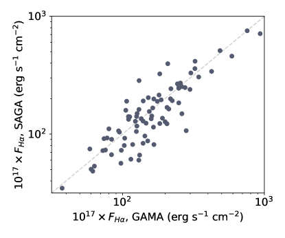
Figure 14: H$\alpha$ fluxes as measured from GAMA DR4 versus H$\alpha$ fluxes for the same galaxies as measured from SAGA AAT/2dF spectra. Note that these are spectra for which the underlying source spectrum is not the same, as opposed to Figure 13.

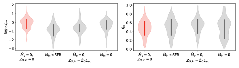
Figure 15: A comparison in inferred parameter distributions for our fiducial model (red, $\dot{M}_{g}=0$) and three alternate models for gas accretion (grey). The vertical line in each distribution shows the range from the 16^th to the 84^th percentile of the posterior. We consider a model where accretion is proportional to SFR (middle distribution in each panel), where accretion balances mass loss in the gas reservoir using gas from the CGM (second from right in each panel), and where there is no accretion of gas at all (rightmost in each panel). In all cases, we find no evidence for a systematic shift in our inferred parameters beyond the fiducial inference uncertainties.

Appendix B Alternate Models of Gas Inflow

Gas accretion in the last $\sim$2.5 Gyr onto the low-mass galaxies in our sample is an interesting if poorly constrained component of the baryon cycle. Though understanding these inflows is of significant scientific interest, in this work we will simply interrogate whether our assumptions about accretion will significantly affect the outcome of our inference. Another way to frame this section is to ask whether our inference can inform our understanding of recent gas inflows into low-mass galaxies; we conclude that the inference is not sensitive to choices about inflows, and leave the editorial evaluation of whether that is a boon or drawback to the reader.

As mentioned in the main text of Section 4, we consider three models for gas accretion in this Appendix. First, we consider a model where the rate of pristine gas inflow scales with the SFR, i.e.

$$M_{\rm in}=\alpha\dot{M}_{\star},$$ (B1)

where $\alpha$ is an additional free parameter in our inference. This relationship between inflow and SFR has been suggested in the literature for disks in equilibrium (Schmidt et al., 2016; Krumholz et al., 2018).

Next, we consider a model in which no inflow is included, i.e. $\dot{M}_{\rm in}=0$. This will induce a negative time derivative of gas mass, $\dot{M}_{g}<0$, since gas is either converted to stellar mass or expelled from the galaxy.

For the last inflow models, we consider the steady-state solution, following Fielding et al. (2017) in defining the steady-state set-up for gas accretion as in our fiducial model:

$$\begin{split}\dot{M}_{\rm in}&=\dot{M}_{\rm out}+\dot{M}_{\star}\\ &=(1+\eta_{\rm m}{})\dot{M}_{\star},\end{split}$$ (B2)

which, given that $\dot{M}_{g}=\dot{M}_{\rm in}-\dot{M}_{\rm out}-\dot{M}_{\star}$ implies that $\dot{M}_{g}=0$ when we recall that $\eta_{\rm m}{}=\dot{M}_{\rm out}/\dot{M}_{\star}$. We propose two variations on this simple accretion model: one where the incoming gas is pristine ($Z_{O}=0$, the cosmological inflow case), and one where the incoming gas is cooled from the CGM. It is both theoretically expected and observationally realized that the metallicity of the CGM should be generally lower than that of the ISM (Kacprzak et al., 2019); we adopt a simple approximation for the relationship between the metallicity of the ISM and CGM wherein the metallicity difference is approximately equal to the expected change in oxygen abundance of the ISM over a characteristic recycling time. This recycling time is the timescale over which fountain flows launched into the CGM from the ISM are expected to cool and accrete back onto the ISM; we adopt $t_{rec}=0.5$ Gyr following the results of Anglés-Alcázar et al. (2017) in the relevant mass range.

In all three cases, we find that our inference of $\eta_{\rm m}{}$ and $f_{21}{}$ does not shift beyond the 16^th to 84^th percentile region of our fiducial posterior distributions, as shown in Figure 15. Our estimate of $a_{\rm SFH}{}$ is also unaffected; this parameter is not expected to be strongly affected by changes in gas inflow prescriptions. We thus conclude that the results presented in this work are not sensitive to and cannot distinguish between models of recent gas inflow. Part of this may be that the recycling time of fountain flows launched from these galaxies into the CGM is not long compared to the timesteps (or redshift bins) adopted in the study. Thus, much of the gas that will be reaccreted into the ISM from the CGM has already done so in the $\Delta t_{lb}\sim 400$ Myr that defines our movement from one redshift bin to the next.

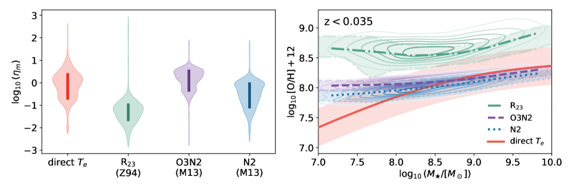
Figure 16: Left: A comparison of the effect of our choice of metallicity calibrator on our inferred mass-loading factor (left) and 21cm-bright gas fraction (right). As in Figure 15, we show our fiducial results in red and our alternate metallicity calibrators in grey. We show the ${\text{R}_{23}}$ calibration of Zaritsky et al. (1994) at center and the O3N2 calibration of Marino et al. (2013) at right. We find that the O3N2 strongline calibration produces a mass-loading factor that is consistent with our direct-$T_{e}$ fiducial model ($\eta_{\rm m}(\text{O3N2})=1.8^{+2.1}_{-1.3}$), and that the ${\text{R}_{23}}$ calibration produces a mass-loading factor somewhat lower than our fiducial model ($\eta_{\rm m}(\rm R_{23})=0.06^{+0.06}_{-0.04}$). Right: The $z<0.035$ mass-metallicity relation for each calibrator as compared to our mass-metallicity fit from Figure 5, which has been validated against auroral line metallicity estimates from the local Universe.

Appendix C Alternate Gas-Phase Metallicity Estimates

In addition to alternative models of inflow, it is useful to understand the impact of our choice of metallicity calibration on our estimate of the mass-loading factor. In our fiducial model, we use direct temperature metallicity estimates in order to alleviate potential biases resulting from the considerable offsets present between different strongline calibrations in the literature (for an overview, see Kewley et al. 2019). However, as discussed in Section 3, adopting a metallicity estimation method that relies upon the detection of the weak auroral lines may introduce its own biases.

To understand the implication of using direct temperature metallicities on our estimate of the mass-loading factor, we rerun our fiducial model using three different strong-line ratio calibrations from the literature. We use three strong-line ratios for this exercise: $\rm R_{23}\equiv[F({\rm[OII]\lambda 3727\rm\AA})+F({\rm[OII]\lambda 3729\rm\AA})+F({\rm[OIII]\lambda 4959\rm\AA})+F({\rm[OIII]\lambda 5007\rm\AA})]/F({\rm H\beta})$, O3N2 $\equiv[F({\rm[OIII]\lambda 5007\rm\AA})/F({\rm H\beta})]/[F({\rm[NII]\lambda 6583\AA})/F({\rm H\alpha})]$, and N2 $\equiv F({\rm[NII]\lambda 6583\AA})/F({\rm H\alpha})$. We adopt the $\rm R_{23}$ calibration of Zaritsky et al. (1994) and the O3N2 and N2 calibrations from Marino et al. (2013):

$$(\log_{10}[\text{O/H}]+12)_{\text{Z94}}=9.265-0.33\log_{10}(\rm R_{23})-0.202\log_{10}(\rm R_{23})^{2}-0.207\log_{10}(\rm R_{23})^{3}-0.333\log_{10}(\rm R_{23})^{4}$$ (C1a)

$$(\log_{10}[\text{O/H}]+12)_{\rm M13,N2}=8.743+0.462\log_{10}(\text{N2})$$ (C1b)

$$(\log_{10}[\text{O/H}]+12)_{\rm M13,O3N2}=8.533-0.214\log_{10}(\text{O3N2})$$ (C1c)

We propagate errors on the metallicities via standard propagation of errors from the uncertainty on the measured line fluxes. Only metallicities derived from galaxies whose H$\beta$ and [O III]$\lambda$4959Å fluxes are measured with a $\text{SNR}>5$ are included in the model; the remaining galaxies at $z<0.035$ are assigned metallicities from the best-fit mass-metallicity relation as in the fiducial model.

In Figure 16 we show the posterior distributions of $\eta_{\rm m}{}$ and $f_{21}{}$ for both our fiducial run (red and left in each panel) and the strong-line calibration runs (grey). We find that the two strong-line metallicity calibrations of Marino et al. (2013) produce estimates of $\eta_{\rm m}{}$ that are in good agreement with our fiducial model ($\eta_{\rm m}(\text{O3N2})=1.8^{+2.1}_{-1.3}$ and $\eta_{\rm m}(\text{N2})=0.35^{+0.78}_{-0.35}$), while the $R_{23}$ calibration of Zaritsky et al. (1994) is best-fit by a somewhat smaller mass-loading factor ($\eta_{\rm m}(\rm R_{23})=0.06^{+0.06}_{-0.04}$). The $\rm R_{23}$-based estimate of the mass-loading factor is in mild tension with our fiducial result: $\langle\eta_{\rm m}(\rm T_{e})\rangle_{10}\approx\langle\eta_{\rm m}(\rm R_{23})\rangle_{87}$ where $\langle\rangle_{X}$ denotes the $X^{\rm th}$ percentile of the posterior.

The tension between the $\rm R_{23}$-based calibration and the other methods can be understood when we consider that the Zaritsky et al. (1994) calibration predicts gas-phase metallicities $\sim 0.5$ dex higher than the direct temperature metallicity method and Marino et al. (2013) calibrations (see also Figure 2 of Kewley & Ellison 2008), as shown in the right panel of Figure 16. If we take the limiting case where the strong-line calibrations simply represent a constant shift in oxygen mass fraction, it is straightforward to show that a positive shift in $Z_{O}$ (that is, $Z_{O}({\rm Z94})=Z_{O}({\rm T_{e}})+\Delta Z_{O}({\rm Z94})$ where $\Delta Z_{O}({\rm Z94})>0$) will result in a lower estimated mass-loading factor if all other parameters are held fixed.

From this exercise we have demonstrated two points salient to the main analysis of this work. First, we have shown that strong-line calibrators produce mass-loading factors consistent with or lower than the direct temperature method. This is especially important when we consider that theoretical predictions of the mass-loading are, in general, significantly higher than observational estimates. The mass-loading factor produced by the strong-line calibrator that produces the results that diverge the most from our fiducial $\eta_{\rm m}$ estimate does not favor the high mass-loading factors used in many contemporary simulations of galaxy evolution (see Section 6.2). Second, we find that the absolute calibration of our metallicity estimates does significantly impact our inferred mass-loading factor. This finding supports our decision to use the direct temperature metallicity method to estimate gas-phase metallicities in the main text of this work, as direct-$T_{e}$ metallicities can be more easily validated against analogous results from the literature and do not suffer from the large offsets seen in strong-line calibrations.

Appendix D Inferring Total Gas Masses via a fixed Star Formation Efficiency

A galaxy’s gas reservoir and its star formation are, of course, causally linked. In our fiducial approach, we estimate H I mass via the measured $M_{\star}-M_{\rm HI}$ relation of Bradford et al. (2015). Another way that one may consider assigning H I masses to the galaxies in our reference sample is by assuming the star formation efficiency (here defined as $\epsilon=\text{SFR}/M_{\rm HI}$) of the galaxies rather than their $M_{\star}-M_{\rm HI}$ relation. Star formation efficiency is relatively constant across the stellar mass range probed by our sample, albeit with significant scatter (Huang et al., 2012; Durbala et al., 2020)

Neither method of assigning $M_{\rm HI}$ to galaxies is perfect: assuming the Bradford et al. (2015) relationship between stellar mass and H I mass overestimates the variance in the H I mass distribution at fixed stellar mass and SFR due to unaccounted-for covariance between H I mass and SFR, while assuming a fixed star formation efficiency places a very strong assumption about the relationship between past and current star formation by directly linking the total fuel for star formation to the star formation at $z=0$. Moreover, it has been shown that the overall structure of low-mass galaxies contributes significantly to their star formation efficiency (see, e.g. de los Reyes & Kennicutt, 2019; Ostriker & Kim, 2022); assuming the same SFE for all galaxies in our reference sample would also be an oversimplification. As an exercise in understanding the implications of our choice, we have rerun our inference using a fixed SFE where $\log_{10}\epsilon\sim\mathcal{N}(-10,0.5)$ based on SFE measurements by Huang et al. (2012) and find that it does not affect the outcome of this analysis.

Appendix E Observed and Predicted Summary Statistics in $M_{\star}$-$Z_{O}$-SFR-z space

To supplement the model optimization described in Section 4 and shown in Figure 7 and Figure 8, we consider a brief exercise in model validation below. In Figure 17, we simply show the observed redshift evolution of the median of each of our observable quantities — stellar mass, star formation rate, and gas-phase metallicity — for our observed sample and model predictions.

Here we are considering the total observed evolution, and the trends shown in Figure 17 are not indicative of the underlying physical shift in the median value of the measured quantities. We find that our model (blue) is able to explain the trend in the observed redshift evolution of the median star formation rate (middle) and gas-phase metallicity (right) to the precision of the 90% confidence interval on the sample median. The observed evolution of the stellar mass does deviate from the predicted sample evolution by more than the extent of the 90% confidence interval, but because the offset is small relative to the stellar mass range probed we conclude that the model is sufficient to describe the observed evolution of our sample in $M_{\star}$-SFR-$Z_{O}$ space.

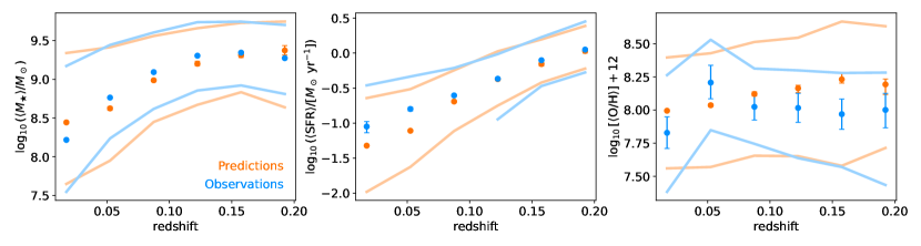
Figure 17: Redshift versus the observed (blue) and predicted (orange) samples in stellar mass (left), star formation rate (middle), and gas-phase metallicity (right). In each panel, the errorbars show the 90% confidence interval on our estimate of the median and the curves indicate the 16^th and 84^th percentiles of the distribution. We find that our model successfully traces the observed shift in our observed sample as a function of redshift, though we stress to the reader that this figure reflects observational rather than physical redshift evolution.

Appendix F Aperture Effects

One observational uncertainty that has persisted across studies of metallicity relations at higher masses has been the fiber covering fraction of the targets. The problem of fiber coverage is ameliorated in the case of the SAGA galaxies due to the small on-sky sizes of our targets (compared to, for example, the higher mass SDSS sample of Mannucci et al. 2010). It is nevertheless important to understand to what degree an aperture effect could influence our results. To do so we perform a simple partial correlation analysis — that is, we consider whether there is evidence for a correlation between gas-phase metallicity and redshift beyond that which can be explained by correlations between each variable and on-sky size.

We expect to see a correlation between both on-sky size and metallicity (due to the correlation between size and stellar mass) and between on-sky size and redshift (due to the relation between angular diameter distance and redshift). To test whether redshift and gas-phase metallicity are correlated beyond what would be implied by their correlations with on-sky size, we compute the linear regression of gas-phase metallicity with respect to on-sky size (left panel of Figure 18) and the linear regression of redshift with respect to on-sky size (middle panel of Figure 18). If the observed correlation between redshift and gas-phase metallicity is driven only by fiber coverage fraction, then we would expect the residuals of these linear regressions to be uncorrelated. Here we restrict our sample to galaxies with stellar masses exceeding $\log_{10}(M_{\star}/M_{\odot})$$>8.9$, the median stellar mass of our sample with auroral line metallicity measurements. We do so to probe a narrower range of the mass–metallicity relation, which we expect to lessen the correlation between all three variables considered due to lower mass galaxies dropping out of the sample.

We see a moderate negative correlation (r=-0.45, in line with the trend seen in the main body of this work), indicating that redshift and gas-phase metallicity are correlated independently of on-sky size. We also computed the linear regression of gas-phase metallicity and on-sky size with respect to redshift to test whether there is evidence for on-sky size and gas-phase metallicity being correlated independently of redshift and found that the correlation is very weak (r=-0.08). From this test, we conclude that our results are not due to a fiber coverage fraction that varies with redshift.

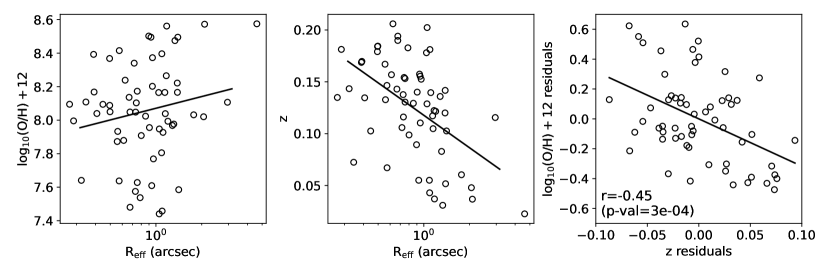
Figure 18: The results of a partial correlation analysis to demonstrate that redshift and gas-phase metallicity are correlated independently of each variable’s correlation with on-sky size. At left we show effective on-sky radius versus gas-phase metallicity, where the black line shows the result of a linear regression of gas-phase metallicity with respect to effective radius. In the middle panel, we show the same but for redshift and effective radius. At right, we show the residuals of each linear regression; if the correlation between redshift and gas-phase metallicity come from a correlation with effective radius then these residuals should be uncorrelated. We find evidence for a moderate negative correlation (r=-0.45, p-value$<10^{-3}$ where the null hypothesis is that the residuals are uncorrelated and normally distributed). In each panel, we show only galaxies with stellar masses exceeding $\log_{10}(M_{\star}/M_{\odot})$$>8.9$.

Appendix G The Contribution of Environment

The main scope of this paper is not to assess the detailed environment of the SAGA background galaxies, but it is important to our analysis to assess whether the environment of the galaxies in our sample is changing as a function of redshift. The overall satellite fraction for galaxies in a given stellar mass range is not expected to change significantly over $0<z<0.21$ (Conroy et al., 2006; Mandelbaum et al., 2006; Guo et al., 2019; Shuntov et al., 2022), but we would like to confirm that this is true for the galaxies in our photometric selection.

To roughly assess the contribution of satellites to our sample, we consider only the SAGA background spectra that overlap the GAMA G09, G12, or G15 regions. We then look for potential hosts of the SAGA galaxies from both the GAMA and NASA Sloan Atlas (NSA) catalogs, where we define a potential host as a galaxy with $M_{r}<-22$ using the source catalog photometry that lies within a projected distance of 2.5 Mpc of the SAGA galaxy with a velocity difference of $\Delta v<1000\ {\rm km\ s^{-1}}$. We expect GAMA to be complete over our redshift range given the cut in absolute magnitude (Baldry et al., 2018), but the overlapping SAGA hosts are close to or cross the edge of the GAMA footprint. We thus expect the GAMA hosts to be complete only at around $z>0.14$, where the projected comoving distance per 0.5 deg is twice our projected distance cut. Conversely, although the NSA is complete for our low-redshift hosts, the catalog only extends out to $z=0.055$.

We can nevertheless use this combination of datasets to determine whether the satellite fraction (the fraction of galaxies that are a satellite) changes significantly with redshift. In Figure 19 we show the satellite fraction as a function of redshift, where the region at $0.055<z<0.14$ is covered by a grey shaded hatch to indicate the region of GAMA and NSA host catalog incompleteness. We find that the satellite fraction in our sample is consistent with a constant value of around 6%. This is somewhat lower than the satellite fractions found for the full low-mass galaxy population in simulations (Kravtsov et al., 2004; Conroy et al., 2006; Mandelbaum et al., 2006; Guo et al., 2019; Shuntov et al., 2022), which is consistent with the well-established idea that the quenched low-mass galaxy population is dominated by satellites (Geha et al., 2012).

For the purview of this analysis, the salient point of the exercise above is that the satellite fraction is consistent with a low and constant value over the redshift range considered in this work. Thus, we expect that neither differential evolution of star-forming satellite galaxies nor the overdensity of satellites associated with the SAGA hosts at $z<0.01$ have influenced the results presented in this work.

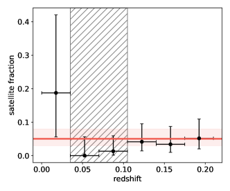
Figure 19: The estimated fraction of SAGA background galaxies in the present work that are satellites as estimated from a joint match to the GAMA and NSA catalogs for galaxies at $M_{r}<-22$. We shade the region at $0.055<z<0.14$ to show the redshift space where neither NSA nor GAMA is complete. The uncertainties on the satellite fraction are computed as confidence intervals for a binomial population using a Jeffreys Bayesian interval. The red line and shaded region show the satellite fraction computed across $(z<0.055)\lor(z>0.14)$.

References

- jon (2001) 2001, SciPy: Open source scientific tools for Python. http://www.scipy.org/
- Andrews & Martini (2013) Andrews, B. H., & Martini, P. 2013, ApJ, 765, 140, doi: 10.1088/0004-637X/765/2/140
- Anglés-Alcázar et al. (2017) Anglés-Alcázar, D., Faucher-Giguère, C.-A., Kereš, D., et al. 2017, MNRAS, 470, 4698, doi: 10.1093/mnras/stx1517
- Astropy Collaboration et al. (2013) Astropy Collaboration, Robitaille, T. P., Tollerud, E. J., et al. 2013, A&A, 558, A33, doi: 10.1051/0004-6361/201322068
- Baldry et al. (2010) Baldry, I. K., Robotham, A. S. G., Hill, D. T., et al. 2010, MNRAS, 404, 86, doi: 10.1111/j.1365-2966.2010.16282.x
- Baldry et al. (2018) Baldry, I. K., Liske, J., Brown, M. J. I., et al. 2018, MNRAS, 474, 3875, doi: 10.1093/mnras/stx3042
- Barbary (2021) Barbary, K. 2021, extinction: Dust extinction laws, Astrophysics Source Code Library, record ascl:2102.026. http://ascl.net/2102.026
- Bell et al. (2003) Bell, E. F., McIntosh, D. H., Katz, N., & Weinberg, M. D. 2003, ApJS, 149, 289, doi: 10.1086/378847
- Berg et al. (2019) Berg, D. A., Erb, D. K., Henry, R. B. C., Skillman, E. D., & McQuinn, K. B. W. 2019, ApJ, 874, 93, doi: 10.3847/1538-4357/ab020a
- Berg et al. (2012) Berg, D. A., Skillman, E. D., Marble, A. R., et al. 2012, ApJ, 754, 98, doi: 10.1088/0004-637X/754/2/98
- Besla et al. (2018) Besla, G., Patton, D. R., Stierwalt, S., et al. 2018, MNRAS, 480, 3376, doi: 10.1093/mnras/sty2041
- Bouché et al. (2010) Bouché, N., Dekel, A., Genzel, R., et al. 2010, ApJ, 718, 1001, doi: 10.1088/0004-637X/718/2/1001
- Bradford et al. (2015) Bradford, J. D., Geha, M. C., & Blanton, M. R. 2015, ApJ, 809, 146, doi: 10.1088/0004-637X/809/2/146
- Brook et al. (2014) Brook, C. B., Di Cintio, A., Knebe, A., et al. 2014, ApJ, 784, L14, doi: 10.1088/2041-8205/784/1/L14
- Bullock & Boylan-Kolchin (2017) Bullock, J. S., & Boylan-Kolchin, M. 2017, ARA&A, 55, 343, doi: 10.1146/annurev-astro-091916-055313
- Calzetti (2013) Calzetti, D. 2013, in Secular Evolution of Galaxies, ed. J. Falcón-Barroso & J. H. Knapen, 419, doi: 10.48550/arXiv.1208.2997
- Calzetti et al. (2000) Calzetti, D., Armus, L., Bohlin, R. C., et al. 2000, ApJ, 533, 682, doi: 10.1086/308692
- Campbell et al. (1986) Campbell, A., Terlevich, R., & Melnick, J. 1986, MNRAS, 223, 811, doi: 10.1093/mnras/223.4.811
- Cardelli et al. (1989) Cardelli, J. A., Clayton, G. C., & Mathis, J. S. 1989, ApJ, 345, 245, doi: 10.1086/167900
- Cardona-Barrero et al. (2023) Cardona-Barrero, S., Di Cintio, A., Battaglia, G., Macciò, A. V., & Taibi, S. 2023, MNRAS, 519, 1545, doi: 10.1093/mnras/stac3243
- Carigi (1994) Carigi, L. 1994, ApJ, 424, 181, doi: 10.1086/173881
- Carlsten et al. (2022) Carlsten, S. G., Greene, J. E., Beaton, R. L., Danieli, S., & Greco, J. P. 2022, ApJ, 933, 47, doi: 10.3847/1538-4357/ac6fd7
- Carlsten et al. (2021) Carlsten, S. G., Greene, J. E., Peter, A. H. G., Beaton, R. L., & Greco, J. P. 2021, ApJ, 908, 109, doi: 10.3847/1538-4357/abd039
- Carr et al. (2022) Carr, C., Bryan, G. L., Fielding, D. B., Pandya, V., & Somerville, R. S. 2022, Regulation of Star Formation by a Hot Circumgalactic Medium, Tech. rep., doi: 10.48550/arXiv.2211.05115
- Chabrier (2003) Chabrier, G. 2003, PASP, 115, 763, doi: 10.1086/376392
- Chen et al. (2023) Chen, Y., Jones, T., Sanders, R., et al. 2023, Nature Astronomy, 7, 771, doi: 10.1038/s41550-023-01953-7
- Chisholm et al. (2017) Chisholm, J., Orlitová, I., Schaerer, D., et al. 2017, A&A, 605, A67, doi: 10.1051/0004-6361/201730610
- Conroy et al. (2006) Conroy, C., Wechsler, R. H., & Kravtsov, A. V. 2006, ApJ, 647, 201, doi: 10.1086/503602
- Cook et al. (2014) Cook, D. O., Dale, D. A., Johnson, B. D., et al. 2014, MNRAS, 445, 899, doi: 10.1093/mnras/stu1787
- Curti et al. (2017) Curti, M., Cresci, G., Mannucci, F., et al. 2017, MNRAS, 465, 1384, doi: 10.1093/mnras/stw2766
- Curti et al. (2020) Curti, M., Mannucci, F., Cresci, G., & Maiolino, R. 2020, MNRAS, 491, 944, doi: 10.1093/mnras/stz2910
- Dalcanton (2007) Dalcanton, J. J. 2007, ApJ, 658, 941, doi: 10.1086/508913
- Dale et al. (2009) Dale, D. A., Cohen, S. A., Johnson, L. C., et al. 2009, ApJ, 703, 517, doi: 10.1088/0004-637X/703/1/517
- Danieli et al. (2022) Danieli, S., Greene, J. E., Carlsten, S., et al. 2022, arXiv e-prints, arXiv:2210.14233, doi: 10.48550/arXiv.2210.14233
- Darragh-Ford et al. (2022) Darragh-Ford, E., Wu, J. F., Mao, Y.-Y., et al. 2022, arXiv e-prints, arXiv:2212.07433, doi: 10.48550/arXiv.2212.07433
- Davé et al. (2012) Davé, R., Finlator, K., & Oppenheimer, B. D. 2012, MNRAS, 421, 98, doi: 10.1111/j.1365-2966.2011.20148.x
- de los Reyes et al. (2015) de los Reyes, M. A., Ly, C., Lee, J. C., et al. 2015, AJ, 149, 79, doi: 10.1088/0004-6256/149/2/79
- de los Reyes & Kennicutt (2019) de los Reyes, M. A. C., & Kennicutt, Robert C., J. 2019, ApJ, 872, 16, doi: 10.3847/1538-4357/aafa82
- Dekel & Silk (1986) Dekel, A., & Silk, J. 1986, ApJ, 303, 39, doi: 10.1086/164050
- Del Popolo & Pace (2016) Del Popolo, A., & Pace, F. 2016, Ap&SS, 361, 162, doi: 10.1007/s10509-016-2742-z
- Di Teodoro & Peek (2021) Di Teodoro, E. M., & Peek, J. E. G. 2021, ApJ, 923, 220, doi: 10.3847/1538-4357/ac2cbd
- Driver et al. (2009) Driver, S. P., Norberg, P., Baldry, I. K., et al. 2009, Astronomy and Geophysics, 50, 5.12, doi: 10.1111/j.1468-4004.2009.50512.x
- Durbala et al. (2020) Durbala, A., Finn, R. A., Crone Odekon, M., et al. 2020, AJ, 160, 271, doi: 10.3847/1538-3881/abc018
- El-Badry et al. (2016) El-Badry, K., Wetzel, A., Geha, M., et al. 2016, ApJ, 820, 131, doi: 10.3847/0004-637X/820/2/131
- El-Badry et al. (2018) El-Badry, K., Bradford, J., Quataert, E., et al. 2018, MNRAS, 477, 1536, doi: 10.1093/mnras/sty730
- Emami et al. (2019) Emami, N., Siana, B., Weisz, D. R., et al. 2019, ApJ, 881, 71, doi: 10.3847/1538-4357/ab211a
- Fielding et al. (2017) Fielding, D., Quataert, E., McCourt, M., & Thompson, T. A. 2017, MNRAS, 466, 3810, doi: 10.1093/mnras/stw3326
- Foreman-Mackey et al. (2013) Foreman-Mackey, D., Hogg, D. W., Lang, D., & Goodman, J. 2013, PASP, 125, 306, doi: 10.1086/670067
- Fumagalli et al. (2011) Fumagalli, M., da Silva, R. L., & Krumholz, M. R. 2011, ApJ, 741, L26, doi: 10.1088/2041-8205/741/2/L26
- Gao et al. (2018) Gao, Y., Bao, M., Yuan, Q., et al. 2018, ApJ, 869, 15, doi: 10.3847/1538-4357/aae9ef
- Geha et al. (2012) Geha, M., Blanton, M. R., Yan, R., & Tinker, J. L. 2012, ApJ, 757, 85, doi: 10.1088/0004-637X/757/1/85
- Geha et al. (2017) Geha, M., Wechsler, R. H., Mao, Y.-Y., et al. 2017, ApJ, 847, 4, doi: 10.3847/1538-4357/aa8626
- Ginsburg et al. (2019) Ginsburg, A., Sipőcz, B. M., Brasseur, C. E., et al. 2019, AJ, 157, 98, doi: 10.3847/1538-3881/aafc33
- González Delgado et al. (1999) González Delgado, R. M., Leitherer, C., & Heckman, T. M. 1999, ApJS, 125, 489, doi: 10.1086/313285
- Governato et al. (2012) Governato, F., Zolotov, A., Pontzen, A., et al. 2012, MNRAS, 422, 1231, doi: 10.1111/j.1365-2966.2012.20696.x
- Grossauer et al. (2015) Grossauer, J., Taylor, J. E., Ferrarese, L., et al. 2015, ApJ, 807, 88, doi: 10.1088/0004-637X/807/1/88
- Guo et al. (2019) Guo, H., Yang, X., Raichoor, A., et al. 2019, The Astrophysical Journal, 871, 147, doi: 10.3847/1538-4357/aaf9ad
- Hägele et al. (2006) Hägele, G. F., Pérez-Montero, E., Díaz, Á. I., Terlevich, E., & Terlevich, R. 2006, MNRAS, 372, 293, doi: 10.1111/j.1365-2966.2006.10856.x
- Haynes et al. (2018) Haynes, M. P., Giovanelli, R., Kent, B. R., et al. 2018, ApJ, 861, 49, doi: 10.3847/1538-4357/aac956
- Heckman et al. (2015) Heckman, T. M., Alexandroff, R. M., Borthakur, S., Overzier, R., & Leitherer, C. 2015, ApJ, 809, 147, doi: 10.1088/0004-637X/809/2/147
- Heiles & Troland (2003) Heiles, C., & Troland, T. H. 2003, ApJ, 586, 1067, doi: 10.1086/367828
- Hu (2019) Hu, C.-Y. 2019, MNRAS, 483, 3363, doi: 10.1093/mnras/sty3252
- Huang et al. (2012) Huang, S., Haynes, M. P., Giovanelli, R., et al. 2012, The Astronomical Journal, 143, 133, doi: 10.1088/0004-6256/143/6/133
- Hughes et al. (2013) Hughes, T. M., Cortese, L., Boselli, A., Gavazzi, G., & Davies, J. I. 2013, A&A, 550, A115, doi: 10.1051/0004-6361/201218822
- Hunter et al. (2012) Hunter, D. A., Ficut-Vicas, D., Ashley, T., et al. 2012, AJ, 144, 134, doi: 10.1088/0004-6256/144/5/134
- Hunter (2007) Hunter, J. D. 2007, Computing in Science & Engineering, 9, 90, doi: 10.1109/MCSE.2007.55
- IRSA (2022) IRSA. 2022, Galactic Dust Reddening and Extinction, IPAC, doi: 10.26131/IRSA537
- Jahn et al. (2022) Jahn, E. D., Sales, L. V., Wetzel, A., et al. 2022, MNRAS, 513, 2673, doi: 10.1093/mnras/stac811
- Kacprzak et al. (2019) Kacprzak, G. G., Pointon, S. K., Nielsen, N. M., et al. 2019, ApJ, 886, 91, doi: 10.3847/1538-4357/ab4c3c
- Kado-Fong et al. (2023) Kado-Fong, E., Geha, M., Mao, Y.-Y., & Wechsler, R. 2023
- Kado-Fong et al. (2020a) Kado-Fong, E., Greene, J. E., Greco, J. P., et al. 2020a, AJ, 159, 103, doi: 10.3847/1538-3881/ab6ef3
- Kado-Fong et al. (2020b) Kado-Fong, E., Greene, J. E., Huang, S., et al. 2020b, ApJ, 900, 163, doi: 10.3847/1538-4357/abacc2
- Kado-Fong et al. (2022a) Kado-Fong, E., Kim, C.-G., Greene, J. E., & Lancaster, L. 2022a, ApJ, 939, 101, doi: 10.3847/1538-4357/ac9673
- Kado-Fong et al. (2021) Kado-Fong, E., Petrescu, M., Mohammad, M., et al. 2021, ApJ, 920, 72, doi: 10.3847/1538-4357/ac15f0
- Kado-Fong et al. (2022b) Kado-Fong, E., Sanderson, R. E., Greene, J. E., et al. 2022b, ApJ, 931, 152, doi: 10.3847/1538-4357/ac6c88
- Kennicutt & Evans (2012) Kennicutt, R. C., & Evans, N. J. 2012, ARA&A, 50, 531, doi: 10.1146/annurev-astro-081811-125610
- Kewley & Ellison (2008) Kewley, L. J., & Ellison, S. L. 2008, The Astrophysical Journal, 681, 1183, doi: 10.1086/587500
- Kewley et al. (2019) Kewley, L. J., Nicholls, D. C., & Sutherland, R. S. 2019, Annual Review of Astronomy and Astrophysics, 57, 511, doi: 10.1146/annurev-astro-081817-051832
- Kim & Ostriker (2018) Kim, C.-G., & Ostriker, E. C. 2018, ApJ, 853, 173, doi: 10.3847/1538-4357/aaa5ff
- Kim et al. (2020) Kim, C.-G., Ostriker, E. C., Somerville, R. S., et al. 2020, ApJ, 900, 61, doi: 10.3847/1538-4357/aba962
- Kisielius et al. (2009) Kisielius, R., Storey, P. J., Ferland, G. J., & Keenan, F. P. 2009, MNRAS, 397, 903, doi: 10.1111/j.1365-2966.2009.14989.x
- Kravtsov et al. (2004) Kravtsov, A. V., Gnedin, O. Y., & Klypin, A. A. 2004, ApJ, 609, 482, doi: 10.1086/421322
- Kroupa (2001) Kroupa, P. 2001, MNRAS, 322, 231, doi: 10.1046/j.1365-8711.2001.04022.x
- Krumholz et al. (2018) Krumholz, M. R., Burkhart, B., Forbes, J. C., & Crocker, R. M. 2018, Monthly Notices of the Royal Astronomical Society, 477, 2716, doi: 10.1093/mnras/sty852
- Leauthaud et al. (2020) Leauthaud, A., Singh, S., Luo, Y., et al. 2020, Physics of the Dark Universe, 30, 100719, doi: 10.1016/j.dark.2020.100719
- Lee et al. (2009a) Lee, J. C., Kennicutt, Robert C., J., Funes, S. J. J. G., Sakai, S., & Akiyama, S. 2009a, ApJ, 692, 1305, doi: 10.1088/0004-637X/692/2/1305
- Lee et al. (2009b) Lee, J. C., Gil de Paz, A., Tremonti, C., et al. 2009b, ApJ, 706, 599, doi: 10.1088/0004-637X/706/1/599
- Lilly et al. (2013) Lilly, S. J., Carollo, C. M., Pipino, A., Renzini, A., & Peng, Y. 2013, The Astrophysical Journal, 772, 119, doi: 10.1088/0004-637X/772/2/119
- Lin & Zu (2023) Lin, Y., & Zu, Y. 2023, MNRAS, 521, 411, doi: 10.1093/mnras/stad502
- Luo et al. (2023) Luo, Y., Leauthaud, A., Greene, J., et al. 2023, arXiv e-prints, arXiv:2305.19310, doi: 10.48550/arXiv.2305.19310
- Ly et al. (2016) Ly, C., Malkan, M. A., Rigby, J. R., & Nagao, T. 2016, ApJ, 828, 67, doi: 10.3847/0004-637X/828/2/67
- Lynden-Bell (1975) Lynden-Bell, D. 1975, Vistas in Astronomy, 19, 299, doi: 10.1016/0083-6656(75)90005-7
- Maiolino & Mannucci (2019) Maiolino, R., & Mannucci, F. 2019, A&A Rev., 27, 3, doi: 10.1007/s00159-018-0112-2
- Mancera Piña et al. (2019) Mancera Piña, P. E., Fraternali, F., Adams, E. A. K., et al. 2019, ApJ, 883, L33, doi: 10.3847/2041-8213/ab40c7
- Mancera Piña et al. (2020) Mancera Piña, P. E., Fraternali, F., Oman, K. A., et al. 2020, MNRAS, 495, 3636, doi: 10.1093/mnras/staa1256
- Mandelbaum et al. (2006) Mandelbaum, R., Seljak, U., Kauffmann, G., Hirata, C. M., & Brinkmann, J. 2006, Monthly Notices of the Royal Astronomical Society, 368, 715, doi: 10.1111/j.1365-2966.2006.10156.x
- Mannucci et al. (2010) Mannucci, F., Cresci, G., Maiolino, R., Marconi, A., & Gnerucci, A. 2010, MNRAS, 408, 2115, doi: 10.1111/j.1365-2966.2010.17291.x
- Mao et al. (2021) Mao, Y.-Y., Geha, M., Wechsler, R. H., et al. 2021, ApJ, 907, 85, doi: 10.3847/1538-4357/abce58
- Marasco et al. (2023) Marasco, A., Belfiore, F., Cresci, G., et al. 2023, A&A, 670, A92, doi: 10.1051/0004-6361/202244895
- Marino et al. (2013) Marino, R. A., Rosales-Ortega, F. F., Sánchez, S. F., et al. 2013, A&A, 559, A114, doi: 10.1051/0004-6361/201321956
- Martin (1998) Martin, C. L. 1998, ApJ, 506, 222, doi: 10.1086/306219
- Martin (1999) —. 1999, ApJ, 513, 156, doi: 10.1086/306863
- Matteucci (2016) Matteucci, F. 2016, in Journal of Physics Conference Series, Vol. 703, Journal of Physics Conference Series, 012004, doi: 10.1088/1742-6596/703/1/012004
- Matteucci (2021) Matteucci, F. 2021, A&A Rev., 29, 5, doi: 10.1007/s00159-021-00133-8
- McKinney (2010) McKinney, W. 2010, in Proceedings of the 9th Python in Science Conference, Vol. 445, Austin, TX, 51–56
- McKinney (2011) McKinney, W. 2011, Python for High Performance and Scientific Computing, 14
- McQuinn et al. (2019) McQuinn, K. B. W., van Zee, L., & Skillman, E. D. 2019, ApJ, 886, 74, doi: 10.3847/1538-4357/ab4c37
- Méndez-Delgado et al. (2023a) Méndez-Delgado, J. E., Esteban, C., García-Rojas, J., Kreckel, K., & Peimbert, M. 2023a, Nature, 618, 249, doi: 10.1038/s41586-023-05956-2
- Méndez-Delgado et al. (2023b) —. 2023b, arXiv e-prints, arXiv:2310.01197, doi: 10.48550/arXiv.2310.01197
- Muratov et al. (2015) Muratov, A. L., Kereš, D., Faucher-Giguère, C.-A., et al. 2015, Monthly Notices of the Royal Astronomical Society, 454, 2691, doi: 10.1093/mnras/stv2126
- Nadler et al. (2020) Nadler, E. O., Wechsler, R. H., Bechtol, K., et al. 2020, ApJ, 893, 48, doi: 10.3847/1538-4357/ab846a
- Nadler et al. (2021) Nadler, E. O., Drlica-Wagner, A., Bechtol, K., et al. 2021, Phys. Rev. Lett., 126, 091101, doi: 10.1103/PhysRevLett.126.091101
- Nelson et al. (2019) Nelson, D., Springel, V., Pillepich, A., et al. 2019, Computational Astrophysics and Cosmology, 6, 2, doi: 10.1186/s40668-019-0028-x
- Newton et al. (2021) Newton, O., Leo, M., Cautun, M., et al. 2021, J. Cosmology Astropart. Phys, 2021, 062, doi: 10.1088/1475-7516/2021/08/062
- Nomoto et al. (2013) Nomoto, K., Kobayashi, C., & Tominaga, N. 2013, ARA&A, 51, 457, doi: 10.1146/annurev-astro-082812-140956
- Oñorbe et al. (2015) Oñorbe, J., Boylan-Kolchin, M., Bullock, J. S., et al. 2015, MNRAS, 454, 2092, doi: 10.1093/mnras/stv2072
- Ostriker & Kim (2022) Ostriker, E. C., & Kim, C.-G. 2022, ApJ, 936, 137, doi: 10.3847/1538-4357/ac7de2
- Pagel & Patchett (1975) Pagel, B. E. J., & Patchett, B. E. 1975, MNRAS, 172, 13, doi: 10.1093/mnras/172.1.13
- Pagel et al. (1992) Pagel, B. E. J., Simonson, E. A., Terlevich, R. J., & Edmunds, M. G. 1992, MNRAS, 255, 325, doi: 10.1093/mnras/255.2.325
- Pandya et al. (2020) Pandya, V., Somerville, R. S., Anglés-Alcázar, D., et al. 2020, ApJ, 905, 4, doi: 10.3847/1538-4357/abc3c1
- Pandya et al. (2021) Pandya, V., Fielding, D. B., Anglés-Alcázar, D., et al. 2021, Monthly Notices of the Royal Astronomical Society, 508, 2979, doi: 10.1093/mnras/stab2714
- Peng et al. (2010) Peng, Y.-j., Lilly, S. J., Kovač, K., et al. 2010, ApJ, 721, 193, doi: 10.1088/0004-637X/721/1/193
- Pequignot et al. (1991) Pequignot, D., Petitjean, P., & Boisson, C. 1991, A&A, 251, 680
- Pérez & Granger (2007) Pérez, F., & Granger, B. E. 2007, Computing in Science and Engineering, 9, 21, doi: 10.1109/MCSE.2007.53
- Pérez-Montero (2017) Pérez-Montero, E. 2017, PASP, 129, 043001, doi: 10.1088/1538-3873/aa5abb
- Pistis et al. (2023) Pistis, F., Pollo, A., Figueira, M., et al. 2023, arXiv e-prints, arXiv:2312.00930, doi: 10.48550/arXiv.2312.00930
- Price-Whelan et al. (2018) Price-Whelan, A. M., Sipőcz, B. M., Günther, H. M., et al. 2018, AJ, 156, 123, doi: 10.3847/1538-3881/aabc4f
- Purcell et al. (2007) Purcell, C. W., Bullock, J. S., & Zentner, A. R. 2007, ApJ, 666, 20, doi: 10.1086/519787
- Rohatgi (2022) Rohatgi, A. 2022, Webplotdigitizer: Version 4.6. https://automeris.io/WebPlotDigitizer
- Romano et al. (2010) Romano, D., Karakas, A. I., Tosi, M., & Matteucci, F. 2010, A&A, 522, A32, doi: 10.1051/0004-6361/201014483
- Rubin et al. (2012) Rubin, K. H. R., Prochaska, J. X., Koo, D. C., & Phillips, A. C. 2012, ApJ, 747, L26, doi: 10.1088/2041-8205/747/2/L26
- Sánchez et al. (2013) Sánchez, S. F., Rosales-Ortega, F. F., Jungwiert, B., et al. 2013, A&A, 554, A58, doi: 10.1051/0004-6361/201220669
- Sanders et al. (2020) Sanders, R. L., Shapley, A. E., Reddy, N. A., et al. 2020, MNRAS, 491, 1427, doi: 10.1093/mnras/stz3032
- Schlafly & Finkbeiner (2011) Schlafly, E. F., & Finkbeiner, D. P. 2011, ApJ, 737, 103, doi: 10.1088/0004-637X/737/2/103
- Schmidt et al. (2016) Schmidt, T. M., Bigiel, F., Klessen, R. S., & de Blok, W. J. G. 2016, MNRAS, 457, 2642, doi: 10.1093/mnras/stw011
- Scott (1992) Scott, D. W. 1992, Multivariate Density Estimation
- Semenov et al. (2021) Semenov, V. A., Kravtsov, A. V., & Gnedin, N. Y. 2021, ApJ, 918, 13, doi: 10.3847/1538-4357/ac0a77
- Shuntov et al. (2022) Shuntov, M., McCracken, H. J., Gavazzi, R., et al. 2022, Astronomy & Astrophysics, 664, A61, doi: 10.1051/0004-6361/202243136
- Stasińska (1990) Stasińska, G. 1990, A&AS, 83, 501
- Steinwandel et al. (2022a) Steinwandel, U. P., Bryan, G. L., Somerville, R. S., Hayward, C. C., & Burkhart, B. 2022a, arXiv e-prints, arXiv:2205.09774, doi: 10.48550/arXiv.2205.09774
- Steinwandel et al. (2023) —. 2023, MNRAS, 526, 1408, doi: 10.1093/mnras/stad2744
- Steinwandel et al. (2022b) Steinwandel, U. P., Kim, C.-G., Bryan, G. L., et al. 2022b, arXiv e-prints, arXiv:2212.03898, doi: 10.48550/arXiv.2212.03898
- Stierwalt et al. (2015) Stierwalt, S., Besla, G., Patton, D., et al. 2015, ApJ, 805, 2, doi: 10.1088/0004-637X/805/1/2
- Storey & Hummer (1995) Storey, P. J., & Hummer, D. G. 1995, MNRAS, 272, 41, doi: 10.1093/mnras/272.1.41
- Storey et al. (2014) Storey, P. J., Sochi, T., & Badnell, N. R. 2014, MNRAS, 441, 3028, doi: 10.1093/mnras/stu777
- Storey & Zeippen (2000) Storey, P. J., & Zeippen, C. J. 2000, MNRAS, 312, 813, doi: 10.1046/j.1365-8711.2000.03184.x
- Taylor et al. (2011) Taylor, E. N., Hopkins, A. M., Baldry, I. K., et al. 2011, MNRAS, 418, 1587, doi: 10.1111/j.1365-2966.2011.19536.x
- Telford et al. (2016) Telford, O. G., Dalcanton, J. J., Skillman, E. D., & Conroy, C. 2016, ApJ, 827, 35, doi: 10.3847/0004-637X/827/1/35
- Van Der Walt et al. (2011) Van Der Walt, S., Colbert, S. C., & Varoquaux, G. 2011, Computing in Science & Engineering, 13, 22
- Vincenzo et al. (2016) Vincenzo, F., Matteucci, F., Belfiore, F., & Maiolino, R. 2016, MNRAS, 455, 4183, doi: 10.1093/mnras/stv2598
- Wetzel et al. (2016) Wetzel, A. R., Hopkins, P. F., Kim, J.-h., et al. 2016, ApJ, 827, L23, doi: 10.3847/2041-8205/827/2/L23
- White & Frenk (1991) White, S. D. M., & Frenk, C. S. 1991, ApJ, 379, 52, doi: 10.1086/170483
- Yates et al. (2020) Yates, R. M., Schady, P., Chen, T. W., Schweyer, T., & Wiseman, P. 2020, A&A, 634, A107, doi: 10.1051/0004-6361/201936506
- Yin et al. (2011) Yin, J., Matteucci, F., & Vladilo, G. 2011, A&A, 531, A136, doi: 10.1051/0004-6361/201015022
- Yin et al. (2023) Yin, J., Shen, S., & Hao, L. 2023, ApJ, 958, 34, doi: 10.3847/1538-4357/acfa6b
- Zahid et al. (2012) Zahid, H. J., Dima, G. I., Kewley, L. J., Erb, D. K., & Davé, R. 2012, ApJ, 757, 54, doi: 10.1088/0004-637X/757/1/54
- Zaritsky et al. (1994) Zaritsky, D., Kennicutt, Robert C., J., & Huchra, J. P. 1994, ApJ, 420, 87, doi: 10.1086/173544
- Zeippen (1982) Zeippen, C. J. 1982, MNRAS, 198, 111, doi: 10.1093/mnras/198.1.111