PICL: Physics Informed Contrastive Learning for Partial Differential Equations

Abstract

Neural operators have recently grown in popularity as Partial Differential Equation (PDEs) surrogate models. Learning solution functionals, rather than functions, has proven to be a powerful approach to calculate fast, accurate solutions to complex PDEs. While much work has been done evaluating neural operator performance on a wide variety of surrogate modeling tasks, these works normally evaluate performance on a single equation at a time. In this work, we develop a novel contrastive pretraining framework utilizing Generalized Contrastive Loss that improves neural operator generalization across multiple governing equations simultaneously. Governing equation coefficients are used to measure ground-truth similarity between systems. A combination of physics-informed system evolution and latent-space model output are anchored to input data and used in our distance function. We find that physics-informed contrastive pretraining improves both accuracy and generalization for the Fourier Neural Operator in fixed-future task, with comparable performance on the autoregressive rollout, and superresolution tasks for the 1D Heat, Burgers’, and linear advection equations.

[inst1]organization=Department of Mechanical Engineering, Carnegie Mellon University,addressline=5000 Forbes Ave, city=Pittsburgh, postcode=1521, state=Pennsylvania, country=USA

[inst2]organization=Department of Biomedical Engineering, Carnegie Mellon University,addressline=5000 Forbes Ave, city=Pittsburgh, postcode=1521, state=Pennsylvania, country=USA [inst3]organization=Machine Learning Department, Carnegie Mellon University,addressline=5000 Forbes Ave, city=Pittsburgh, postcode=1521, state=Pennsylvania, country=USA

1 Introduction

Contrastive learning frameworks have shown great promise in traditional machine learning tasks such as image classification[1, 2], with more recent works extending the applications to molecular property prediction[3] and dynamical systems[4]. While these works generally focus on classes that have distinct boundaries, weighted contrastive learning has been developed for cases where distinct samples are more similar to some samples than others. This has been applied to visual place recognition[5, 6] as well as molecular property prediction[7]. In the case of Partial Differential Equations (PDEs), weighted similarity can be useful in learning multiple operators simultaneously. For example, a system governed by diffusion-dominated Burgers’ equation behaves much more similarly to a system governed by the Heat equation than a system governed by advection-dominated Burgers’ equation, and one model may be trained to learn both systems governed by the heat and Burgers’ equations.

Many neural operators have been developed for various PDE surrogate modeling tasks [8, 9, 10, 11]. Existing works aim to improve simulation speed through super-resolution [12], mesh optimization [13], compressed representation [14, 15, 16, 17]. Despite their promising results, few works have tested generalization across different operator coefficients for a single governing equation, or multiple governing equations. Recently, Physics Informed Token Transformer has shown promise in multi-system learning [18], and the CAPE module[19] has demonstrated the ability to incorporate different equation coefficients with good generalizability. Other works have looked at utilizing neural operators as foundational models This is in line with current numerical methods, where different finite-difference numerical stencils are used for the Heat and Burgers’ equation, for example. However, neither of these works explicitly utilize the differences between systems, instead relying on a data driven approach to simultaneously learn the effect of equation coefficients and prediction. A recent work, PIANO[20], uses operator coefficients, forcing terms, and boundary condition information for contrastive pretraining. While promising, this work applies pretraining to varying systems with the same governing equation, rather than multiple governing equations. Additionally, the PIANO framework does not take into account similarity between different, but similar, systems.

The aim of this work is to develop a contrastive framework that enables a single model to more effectively learn multiple operators by learning from the differences between systems explicitly. This presents a number of challenges related to both the underlying mathematical theory, as well as practical implementation. Namely, distance functions often utilize norms. Euclidean distance, for example, utilizes the L2 norm. However, it is well known that differential operators are unbounded, and therefore have no norm. Cosine similarity, another popular choice, is magnitude invariant, which may not be able to capture different coefficient magnitudes. Practically speaking, if we were to approximate our differential operators with finite difference matrices, we could use a matrix norm to easily define a distance function. However, since we are using a single set of model weights to learn multiple operators, the matrix norm of model weights is the same for each operator, rendering the matrix norm useless for this case. In this work, we develop a novel framework that overcomes these challenges. Our novel contributions are as follows:

• A novel similarity metric between PDE systems

• A novel neural operator based operator distance function

The similarity metric and distance function are combined using Generalized Contrastive Loss[5, 6] to form our framework: Physics Informed Contrastive Learning (PICL). Our contrastive framework is benchmarked using the Fourier Neural Operator (FNO)[9] on popular 1D and PDEs for fixed-future prediction, super-resolution, and autoregressive rollout. Further analysis also shows that models pretrained with PICL are able to clearly distinguish between different systems. PICL shows significant improvement over standard training in fixed-future experiments, maintained performance in super-resolution, and comparable performance in autoregressive rollout. Latent space embeddings from PICL also show clustering of systems that behave similarly.

2 Data Generation

In order to properly assess performance, multiple data sets that represent distinct physical processes are used. In our case, we have the Heat equation (eq. 1), which is a linear parabolic equation, the linear advection equation (eq. 2 which is a linear hyperbolic equation, and Burgers’ equation (eq. 3. Adapting the setup from [21], we generate the 1D data for the homogeneous Heat and Burgers’ equations, with linear advection data being generated analytically.

$$\partial_{t}u-\beta\partial_{xx}u=0$$ (1)

$$\partial_{t}u+\gamma\partial_{x}u=0$$ (2)

$$\partial_{t}u+\alpha\partial_{x}u^{2}-\beta\partial_{xx}u=0$$ (3)

In this case, a large number of sampled coefficients allow us to generate data for many different systems. We use multiple parameters for each equation to generate our diverse data set, given by: $\alpha\in\left\{0.5,1.0,2.0,5.0\right\}$, $\beta\in\left\{0.1,0.2,0.5,1.0,2.0,5.0\right\}$, and $\gamma\in\left\{0.5,1.0,2.0,5.0\right\}$.

The initial condition is given by:

$$u\left(x\right)=\sum_{j=1}^{J}A_{j}\sin\left(\frac{2\pi l_{j}x}{L}+\phi_{j}\right)\\$$ (4)

The parameters $A$, $l$, and $\phi$ can be sampled to give us many initial conditions for each set of system coefficients. In our case, $J=5$ and $L=128$. The parameters are sampled as follows: $A_{j}\sim\mathcal{U}(-0.5,0.5)$, $l_{j}\sim\{1,2,3\}$, $\phi_{j}\sim\mathcal{U}(0,2\pi)$. For the Heat equation, 2000 samples were generated for each $\beta$ value. For Burgers’ equation, 250 samples were generated for each combination of $\alpha$ and $\beta$ values. Lastly, for the linear advection equation, 2000 samples were generated for each combination of $\gamma$ value. Our system was spatially discretized with 200 evenly spaced points and temporally discretized with 200 evenly spaced samples in time. During training both our spatial and temporal discretizations were evenly downsampled to 50 points.

3 Method

The goal of neural operator learning is to learn the mapping $G_{\theta}:\mathcal{A}\to\mathcal{S}$, parameterized by $\theta$, from input function space $\mathcal{A}$ to solution function space $\mathcal{S}$[22]. When looking at specific functions, we can view our operator as acting on a specific input function, $a$, and mapping it to a specific output function $s$, as: $\mathcal{G}_{\theta}(a)\to s$. Specifically, we are learning various operators $\mathcal{G}_{\theta}$, and pretraining in the neural operator latent embeddings, represented by $\mathcal{G}^{\prime}_{\theta}$. However, as previously mentioned, our single set of model weights $\theta$ acts as different operators depending on the input data. While we cannot practically or mathematically utilize the individual operators themselves for our similarity metric or distance function, we can utilize the effect the operators have on our system.

3.1 Generalized Contrastive Loss

In this work, we use the Generalized Constrastive Loss (GCL)[5, 6], given below in equation 5.

$$\mathcal{L}_{GCL}(z_{i},z_{j})=\psi_{i,j}\frac{d(z_{i},z_{j})^{2}}{2}+\left(1-\psi_{i,j}\right)\frac{\text{max}(\tau-d(z_{i},z_{j}),0)^{2}}{2}$$ (5)

The first term aims to minimize distance between similar samples. In the second term, $\tau$ acts as a margin, above which samples are considered to be from different systems. The second term therefore maximizes distance between unlike samples that are below the margin threshold. The key components of this loss function are the distance function between samples, $d(z_{i},z_{j})$, and the similarity metric, $\psi_{i,j}$. While the distance is calculated model with output, known properties from our system are used in the similarity metric. In this case, we use operator coefficients to measure similarity.

3.2 Similarity Metric

In our data generation, we generate multiple trajectories for each combination of equation parameters: $\alpha$, $\beta$, and $\gamma$, which can be stored in a vector as $\theta_{j}=\left[\alpha,\beta,\gamma\right]$. These parameters select which governing equation is being used as well as the governing equation properties. Once we have constructed the weight vector for each system, the novel magnitude-aware cosine similarity is used to calculate similarity between our weight vectors.

$$\psi(\theta_{i},\theta_{j})=\frac{\sqrt{\left|\theta_{i}\cdot\theta_{j}\right|}}{\text{max}\left(\left\lVert\theta_{i}\right\rVert,\left\lVert\theta_{j}\right\rVert\right)}$$ (6)

While similar to cosine similarity, taking the maximum of both input vectors normalizes the output to 1 if the magnitude of the dot product is equal to the magnitude of the larger vector, i.e. the inputs are identical. Magnitude-awareness is critical for PDEs, because, for example, a diffusion dominated Burgers’ system behaves much more similarly to a pure diffusion system than an advection dominated Burgers’ system.

3.3 Physics Informed Distance Metric

Distance metrics between samples play a vital role in contrastive learning, as they enable reliable measurements of similarity. In many cases, euclidean distance or cosine similarity are used. However, in the case of operator learning for PDEs, it is well known that differential operators are unbounded, and therefore a metric cannot be defined. With this in mind, a measure of similarity must utilize additional information outside of the analytical governing equations must be used to measure similarity between systems. When we have different initial conditions for a given system, i.e. different initial sine waves evolving according to the heat equation with diffusion coefficient of 1, we expect that the system evolution will look similar between these different initial conditions. That is, the difference between the first and second frames of these two systems should show a more similar evolution than if one of the systems evolved according to Burger’s equation, for example. This distance, which we call the system distance, is given in equation 7.

$$d_{system}(u_{i},u_{j})=\left[(u_{i}^{t+1}-u_{i}^{t})-(u_{j}^{t+1}-u_{j}^{t})\right]$$ (7)

Since our models are learning the operators themselves, we must also utilize model output so that errors can be backpropagated. Similar to system difference, we can calculate distances between our predicted states, with additional physics information to calculate the next step, given in equation 8.

$$d_{update}(u_{i},u_{j})=\left[F(G^{\prime}_{\theta}(u_{i}))-G^{\prime}_{\theta}(u_{i})\right]$$ (8)

where $F(G^{\prime}_{\theta}(u_{i}))$ is our analytical update operator. In our case, at timestep $t$,

$$F(z^{t})=z^{t}+2\alpha_{z}z\partial_{x}z^{t}+\beta_{z}\partial_{xx}z^{t}+\gamma_{z}\partial_{x}z^{t}=z^{t+1}$$ (9)

for $G^{\prime}_{\theta}(u)=z$ Where each differential operator is calculated with a finite difference approximation given in appendix A. This distance should be similar to $d_{system}$, since they are both after a single timestep, and so we anchor $d_{physics}$ to $d_{sample}$, inspired by triplet loss[23]. Anchoring is done so that our system update distances are not minimized to 0, which does not accurately reflect the effect of the operators. Incorporating physics information here serves two purposes. First, it helps smooth our model output. A very jagged model output would result in large derivatives that would be very different from our input system evolution. Second, it enforces that our predicted states have a similar analytical update to our input data, which helps ensure the representation is similar to our input data.

$$\begin{split}d_{physics}(u_{i},u_{j},z_{i},z_{j})=&\left\lVert d_{system}(u_{i},u_{j})-d_{update}(z_{i},z_{j})\right\rVert^{2}\\ \end{split}$$ (10)

3.4 Training Procedure

We employ a two step training procedure seen in figure 1, where we first use contrastive pretraining and then standard training. In both stages, we train our model end-to-end. During pretraining, we use our PICL contrastive loss function. After pretraining, during fine-tuning, we use a standard training procedure. We do not employ weight-freezing after pretraining because we have empirically found this to have lower predictive accuracy. The training procedure is given in figure 1.

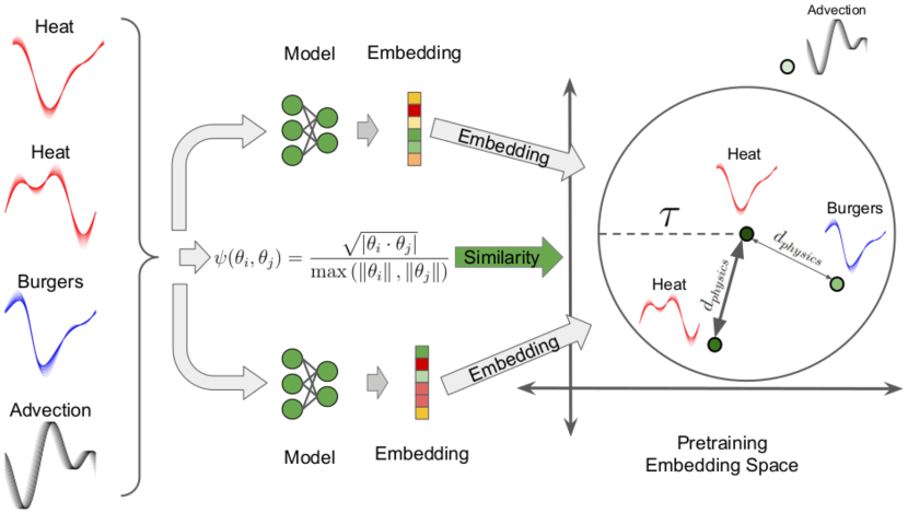
(a) Pretraining procedure.

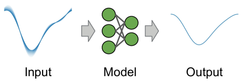
(b) Fine-tuning procedure.

Figure 1: Our two-step training procedure first pretrains on all three equations simultaneously, then fine-tunes on each equation individually. Darker green points represent higher similarity to our Heat sample. Bolder arrows represent stronger attraction between samples in embedding space.

4 Results

PICL is now benchmarked against standard training methods on our 1D data sets. Data is split such that the entirety of a trajectory is either in the train, validation, or test splits, so we do not benchmark models on identical systems in the train and test splits. In each experiment, five random seeds and model initializations were used. Reported values are the mean and standard deviation of these five runs. For all experiments, we compare PICL-pretrained FNO against standard FNO for each of the Heat, Burgers’, and Advection equations individually, as well as all equations in a combined data set. For each experiment, we pretrain using the combined data set, and use the learned model weights after pretraining for fine-tuning on each individual data set, as well as fine-tuning on the combined data set. Hyperparameters for each experiment are given in B.

4.1 Fixed Future Results

In this experiment we aim to learn a mapping from a specified number of initial data frames to a fixed time in the future the operator $\mathcal{G}_{\theta}:a(\cdot,t_{i})|_{i\in\{1,10\}}\to u(\cdot,t_{i})|_{i=50}$ for $\Delta t=0.0603$. For each individual equation we use 5000 random samples, containing all parameter combinations, where every sample has a different initial condition. Results are given in table 1. We see that PICL shows significant improvement over standard training. PICL improves FNO performance by 70% on Heat, 37% on Burgers’, 82% on Advection, and 79% on the combined data sets.

Model	Heat	Burgers’	Advection	Combined
FNO	4.82 $\pm$ 0.14	6.75 $\pm$ 0.08	23.20 $\pm$ 0.60	15.09 $\pm$ 0.48
FNO Pretrained	1.45 $\pm$ 0.13	4.27 $\pm$ 0.31	4.05 $\pm$ 1.16	3.09 $\pm$ 0.23

Table 1: Fixed-Future Pretraining 5000 samples/equation MAE ($\times 10^{-2}$)

4.2 Autoregressive Rollout

To test autoregressive rollout, we first train each model to predict one step in the future given a specified amount of input data. That is, we are learning the operator $\mathcal{G}_{\theta}:a(\cdot,t_{i})|_{i\in[n-9,n]}\to u(\cdot,t_{i})|_{i=n+1}$, again with $\Delta t=0.0603$. After training, we test rollout by using the initial $10$ data frames as input, predicting the next step, then using the $[1,11]$ frames to predict frame $12$, etcetera, until we reach the full trajectory, as in [21]. Results are given in figure 2, where we see FNO pretrained with PICL offers improvement across all of our benchmarks.

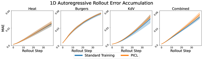
Figure 2: Comparison of autoregressive rollout performance between FNO and FNO pretrained using PICL.

4.3 Zero-Shot Super-Resolution

Lastly, we take the models trained in our fixed-future experiment and evaluate them on higher resolution data. During initial training, we evenly downsampled by a factor of 4, so that we had 50 points to discretize our space. In this experiment, we evaluate on both the original data that has a 200 discretization points, and downsampled data with 100 discretization points. We look at the increase in error as our resolution increases to evaluate super-resolution performance. Results are given in figure 3. We see PICL error increases comparably to baseline, mainting a much lower error for all resolutions.

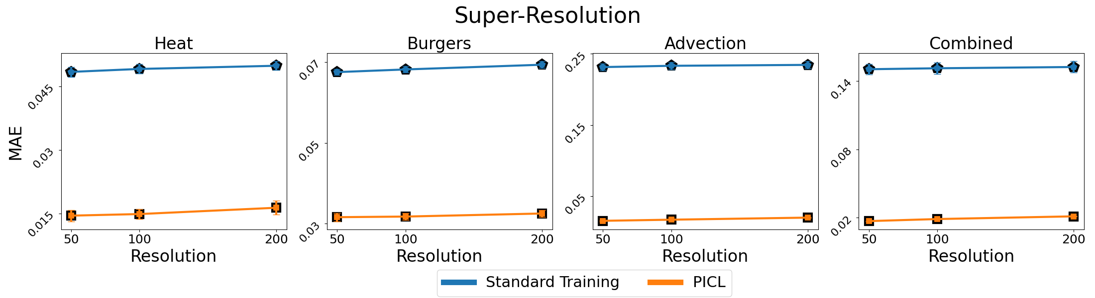
Figure 3: Comparison of super-resolution performance between FNO and FNO pretrained using PICL.

5 Discussion

PICL shows improvement in FNO generalization. For both Heat and Burgers’, we use the 5th-order accurate WENO5 method for data generation. For advection, we use the analytical solution. In all cases, we use a numerical update scheme that is of lower order accuracy. For Heat, we use standard the 2nd-order centered difference scheme in space, and first order backward difference in time. For Burgers’, we use the same 2nd-order centered difference scheme in space for the diffusion term, and the second-order upwind scheme in space for the nonlinear advection term, coupled with a first-order backward difference scheme in time. Lastly, for the linear advection, we use the same second-order upwind in space and first-order backward difference in time. All of these methods have lower order accuracy than what was used for data generation. Despite this, PICL significantly improves results over standard training for fixed-future experiments. Additionally, PICL is robust to stability constraints. In our 1D case, we use a timestep of $\Delta t=0.6030$, with a spatial discretization of $\Delta x=2.5729$ after downsampling. For our upwind scheme, this gives us a CFL number of $\frac{5\Delta t}{\Delta x}=1.17$, larger than the stability constraint of 1. For our diffusion scheme, we obey the stability constraint of $\frac{5\Delta t}{\Delta x^{2}}=0.455<0.5$.

We also check how well PICL allows our model to learn difference between systems by analyzing t-SNE embeddings of our latent representations in figure 4. We see clear regions of both advection and Burgers’ equation embedding in the pink dotted line box and gold dot dashed line box, respectively. While there is no single, large region of heat equation embeddings, we can nevertheless inspect a smaller region, which is outlined by the green dashed line box. Parameter distributions for each region are given in the bar plots below the embeddings scatter plot. Inside of the highlighted region of advection equation embeddings, we see every embedding belongs to a system with advection coefficient of $5$. 99.5% of all such systems are contained inside of this region, indicating excellent separation between advection systems in the embedding space. In the highlighted region of Burgers’ equation embeddings, 67.2% have a nonlinear advection coefficient of $5$. In the Burgers’ region, the diffusion coefficient is approximately evenly distributed, indicating that our model learns that advection-dominated Burgers’ systems have relatively similar behavior, which we intuitively expect. Lastly, the highlighted region of heat equation embeddings shows approximately uniform distribution, and other regions have shown similar results.

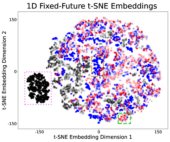
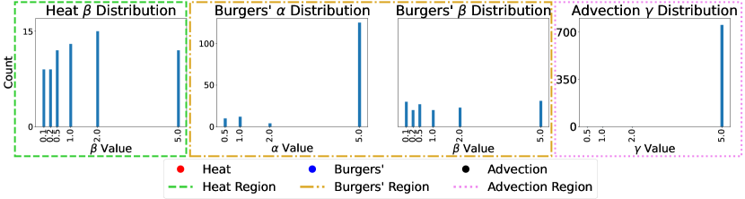
Figure 4: t-SNE of latent embeddings after PICL pretraining and coefficient distributions.

6 Conclusion

PICL offers a novel physics informed contrastive framework that improves FNO generalization on 1D homogenous PDE systems. PICL leverages physics informed updates by anchoring predicted state updates to input data updates. Future works include developing strategies to incorporate both static and time-dependent forcing terms to our distance function. Applying PICL to 2D and 3D systems, and a broader array of equations are also areas of interest. Higher-dimensional systems offer an additional challenge that the magnitude of our distance function can varies significantly more between popular PDE system setups. This, in turn, makes learning the differences between the effects of various operators more challenging.

7 Data Availability

All code and data will be available at https://github.com/CoopLo/PICL.

Appendix A Physics-Informed Updates

For each operator we use a low-order finite-difference scheme to calculate our updates. In each equation $i$ represents the spatial coordinate. For both our linear and nonlinear advection operators we use the upwind scheme since our advection velocity is always positive.

$$\partial_{x}u=\frac{\Delta t}{\Delta x}\left(u_{i}-u_{i-1}\right)$$ (11)

$$\partial_{xx}u=\frac{\Delta t^{2}}{\Delta x^{2}}\left(u_{i+1}-2u_{i}+u_{i-1}\right)$$ (12)

$$u\partial_{x}u=\frac{\Delta t}{\Delta x}u_{i}\left(u_{i}-u_{i-1}\right)$$ (13)

Appendix B Experiment Hyperparameters

For all experiments, we used a 1D FNO with hidden width of 256 and 8 modes that was trained for 500 epochs. Pretraining was done for 500 epochs in the fixed-future experiment, and 100 for the autoregressive rollout experimet. A step learning rate scheduler was used for both pretraining and fine-tuning. In both cases $\tau$ was set to the mean of the current batch of data.

B.1 Fixed-Future Hyperparameters

Table 2: Fine-tuning and Baseline Hyperparameters

Model	Batch Size	Learning Rate	Weight Decay	Scheduler Step	Scheduler $\gamma$	Dropout
FNO	32	1E-2	1E-8	50	0.5	0.1
Pretrain FNO	32	1E-3	1E-8	100	0.5	0.01

Table 3: Pretraining Hyperparameters

Model	Batch Size	Learning Rate	Weight Decay	Scheduler Step	Scheduler $\gamma$	Dropout	$\tau$
Pretrain FNO	512	1E-2	1E-6	50	0.25	0.01	Mean

B.2 Autoregressive Rollout Hyperparameters

Table 4: Fine-tuning and Baseline Hyperparameters

Model	Batch Size	Learning Rate	Weight Decay	Scheduler Step	Scheduler $\gamma$	Dropout
FNO	16	1E-2	1E-8	50	0.5	0.0
Pretrain FNO	16	1E-2	1E-8	50	0.5	0.0

Table 5: Pretraining Hyperparameters

Batch Size	Learning Rate	Weight Decay	Scheduler Step	Scheduler $\gamma$	Dropout	$\tau$
Pretrain FNO	1E-4	1E-7	10	0.5	0.0	Mean

References

-
[1]
T. Chen, S. Kornblith, M. Norouzi, G. Hinton,
A simple framework for
contrastive learning of visual representations, in: H. D. III, A. Singh
(Eds.), Proceedings of the 37th International Conference on Machine Learning,
Vol. 119 of Proceedings of Machine Learning Research, PMLR, 2020, pp.
1597–1607.
URL https://proceedings.mlr.press/v119/chen20j.html -
[2]
K. Sohn, Improved deep metric learning
with multi-class n-pair loss objective, in: D. Lee, M. Sugiyama, U. Luxburg,
I. Guyon, R. Garnett (Eds.), Advances in Neural Information Processing
Systems, Vol. 29, Curran Associates, Inc., 2016.
URL https://papers.nips.cc/paper_files/paper/2016/file/6b180037abbebea991d8b1232f8a8ca9-Paper.pdf -
[3]
Y. Wang, J. Wang, Z. Cao, A. Barati Farimani,
Molecular contrastive
learning of representations via graph neural networks, Nature Machine
Intelligence 4 (3) (2022) 279–287.
doi:10.1038/s42256-022-00447-x.
URL https://doi.org/10.1038/s42256-022-00447-x - [4] R. Jiang, P. Y. Lu, E. Orlova, R. Willett, Training neural operators to preserve invariant measures of chaotic attractors (2023). arXiv:2306.01187.
- [5] M. Leyva-Vallina, N. Strisciuglio, N. Petkov, Generalized contrastive optimization of siamese networks for place recognition (2023). arXiv:2103.06638.
- [6] M. Leyva-Vallina, N. Strisciuglio, N. Petkov, Data-efficient large scale place recognition with graded similarity supervision, in: Proceedings of the IEEE/CVF Conference on Computer Vision and Pattern Recognition (CVPR), 2023, pp. 23487–23496.
-
[7]
Y. Wang, R. Magar, C. Liang, A. Barati Farimani,
Improving molecular
contrastive learning via faulty negative mitigation and decomposed fragment
contrast, Journal of Chemical Information and Modeling 62 (11) (2022)
2713–2725, pMID: 35638560.
arXiv:https://doi.org/10.1021/acs.jcim.2c00495, doi:10.1021/acs.jcim.2c00495.
URL https://doi.org/10.1021/acs.jcim.2c00495 - [8] Z. Li, K. Meidani, A. B. Farimani, Transformer for partial differential equations’ operator learning (2023). arXiv:2205.13671.
- [9] Z. Li, N. Kovachki, K. Azizzadenesheli, B. Liu, K. Bhattacharya, A. Stuart, A. Anandkumar, Fourier neural operator for parametric partial differential equations (2021). arXiv:2010.08895.
-
[10]
L. Lu, P. Jin, G. Pang, Z. Zhang, G. E. Karniadakis,
Learning nonlinear
operators via deeponet based on the universal approximation theorem of
operators, Nature Machine Intelligence 3 (3) (2021) 218–229.
doi:10.1038/s42256-021-00302-5.
URL https://doi.org/10.1038/s42256-021-00302-5 - [11] S. Patil, Z. Li, A. B. Farimani, Hyena neural operator for partial differential equations (2023). arXiv:2306.16524.
-
[12]
D. Shu, Z. Li, A. B. Farimani,
A
physics-informed diffusion model for high-fidelity flow field
reconstruction, Journal of Computational Physics 478 (2023) 111972.
doi:https://doi.org/10.1016/j.jcp.2023.111972.
URL https://www.sciencedirect.com/science/article/pii/S0021999123000670 -
[13]
C. Lorsung, A. Barati Farimani, Mesh
deep Q network: A deep reinforcement learning framework for improving meshes
in computational fluid dynamics, AIP Advances 13 (1), 015026 (01 2023).
arXiv:https://pubs.aip.org/aip/adv/article-pdf/doi/10.1063/5.0138039/16698492/015026\_1\_online.pdf,
doi:10.1063/5.0138039.
URL https://doi.org/10.1063/5.0138039 - [14] A. Hemmasian, A. B. Farimani, Multi-scale time-stepping of partial differential equations with transformers (2023). arXiv:2311.02225.
-
[15]
A. Hemmasian, A. Barati Farimani,
Reduced-order modeling of fluid
flows with transformers, Physics of Fluids 35 (5) (2023) 057126.
arXiv:https://pubs.aip.org/aip/pof/article-pdf/doi/10.1063/5.0151515/17720097/057126\_1\_5.0151515.pdf,
doi:10.1063/5.0151515.
URL https://doi.org/10.1063/5.0151515 -
[16]
Z. Li, S. Patil, D. Shu, A. B. Farimani,
Latent neural PDE solver
for time-dependent systems, in: NeurIPS 2023 AI for Science Workshop, 2023.
URL https://openreview.net/forum?id=iJfPFUvFfy - [17] Z. Li, D. Shu, A. B. Farimani, Scalable transformer for pde surrogate modeling (2023). arXiv:2305.17560.
- [18] C. Lorsung, Z. Li, A. B. Farimani, Physics informed token transformer (2023). arXiv:2305.08757.
- [19] M. Takamoto, F. Alesiani, M. Niepert, Learning neural pde solvers with parameter-guided channel attention (2023). arXiv:2304.14118.
- [20] R. Zhang, Q. Meng, Z.-M. Ma, Deciphering and integrating invariants for neural operator learning with various physical mechanisms (2023). arXiv:2311.14361.
- [21] J. Brandstetter, D. Worrall, M. Welling, Message passing neural pde solvers (2023). arXiv:2202.03376.
-
[22]
N. Kovachki, Z. Li, B. Liu, K. Azizzadenesheli, K. Bhattacharya, A. Stuart,
A. Anandkumar, Neural
operator: Learning maps between function spaces with applications to pdes,
Journal of Machine Learning Research 24 (89) (2023) 1–97.
URL http://jmlr.org/papers/v24/21-1524.html - [23] F. Schroff, D. Kalenichenko, J. Philbin, Facenet: A unified embedding for face recognition and clustering, in: Proceedings of the IEEE Conference on Computer Vision and Pattern Recognition (CVPR), 2015.