Simulation of a Rohksar-Kivelson ladder on a NISQ device
Abstract
We present a quantum-classical algorithm to study the dynamics of the Rohksar-Kivelson plaquette ladder on NISQ devices. We show that complexity is largely reduced using gauge invariance, additional symmetries, and a crucial property associated to how plaquettes are blocked against ring-exchange in the ladder geometry. This allows for an efficient simulation of sizable plaquette ladders with a small number of qubits, well suited for the capabilities of present NISQ devices. We illustrate the procedure for ladders with simulation of up to plaquettes in an IBM-Q machine, employing scaled quantum gates.
I Introduction
Recent years have witnessed spectacular progress in the field of quantum simulators [1, 2], i.e. quantum many-particle systems that simulate other quantum phenomena, which may not be tractable by classical means. This includes applications in disparate fields, ranging from condensed-matter physics [3, 4] to material science and quantum chemistry [5, 6] and high-energy physics [7, 8]. Concerning the latter, quantum simulators open exciting possibilities for the simulation of quantum field theories, and in particular lattice gauge theories with both analogue and digital simulators [9, 10, 11, 7, 8]. A particularly prominent example is provided by the successful simulation of the quantum link Schwinger model [12], a relatively simple model that describes quantum electrodynamics in one space and one time dimension [13, 14, 15, 16, 17, 18].
Despite these extraordinary developments, the analogue simulation of plaquette operators, crucial in the Hamiltonian formulation of lattice gauge theories [19], remains very challenging, since they involve three- and higher-body interactions. Interestingly, it has been recently proposed that the Rydberg blockade in Rydberg configurable arrays could be employed to efficiently simulate plaquette terms, and in particular the Rohksar-Kivelson (RK) model, a two-dimensional U(1) lattice gauge theory which has attracted a large deal of interest due to its relevance in the context of quantum dimer and spin ice theory [20].
Digital simulations may overcome the limitations of analogue devices concerning plaquette operators [21, 22]. However, at the present time, fully fault-tolerant quantum computers are not available. Instead, only noisy intermediate-scale quantum (NISQ) devices [23] have been so far realised, with at most hundreds of qubits, and characterized by sparse connectivity and significant noise and decoherence in the application of quantum gates. Since quantum error correction is not yet possible, a set of error mitigation techniques [24, 25], and algorithms [26] have been specifically designed for NISQ devices. In particular different variational quantum algorithms have been explored for the simulation of the Schwinger model [15, 27].
In this paper, we apply a quantum-classical approach, similar to that employed in Ref. [15], for the study of the real-time dynamics of the RK model in a ladder geometry, possibly the simplest lattice gauge model with plaquette operators. We show that the combination of gauge invariance, symmetrization, and the particular way plaquettes are blocked against ring-exchange in the ladder geometry, allow for an efficient mapping of the RK-ladder dynamics to a small number of qubits, an interesting feature for its implementation in NISQ devices. By employing gate scaling techniques, we show that the procedure allows for the successful simulation of the dynamics of small RK ladders in IBM-Q superconducting quantum computers.
The structure of the paper is as follows. In Sec. II we introduce the RK-ladder model. Section III is devoted to the mapping of the model into a set of effective equations. In Sec. IV we discuss the actual simulation on a quantum computer. Our results are discussed in Sec. V. Finally, we conclude in Sec. VI.
II Rohksar-Kivelson ladder
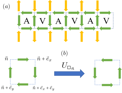
We consider a square ladder, as in Fig. 1 (a). We characterize each ladder vertex by a vector , with denoting the lower and upper legs, respectively. We associate to each link of the ladder a spin- degree of freedom, with two states and . For convenience of the representation, for spins placed in links along the legs we denote those states as and , respectively. Introducing the raising and lowering spin operators acting on the spin placed at the link between the neighboring sites and ( , ), we define for each plaquette (with the top-left vertex of the plaquette, see Fig. 1 (b)) a ring-exchange operator
| (1) |
with and . Given a vortex (antivortex) plaquette state (), where we follow the same clockwise order of Fig. 1 (b), the ring-exchange flips the state as , and . Any other spin configuration, which we denote below as , is blocked, i.e. non-flippable, and . We consider the RK model [28]:
| (2) |
where denotes the sum over all ladder plaquettes. Since , , , then the operator acts as counter of the number of flippable, either or , plaquettes. The RK coupling hence determines the energy penalty resulting from the change in the number of flippable plaquettes. We set below .
We define the local gauge transformation generator at vertex as:
| (3) |
with the projection of the spin placed in between two neighboring sites and . Note that in the ladder geometry, we have to consider virtual spins outside the ladder, which remain fixed during the dynamics (orange arrows in Fig. 1). As a result, the gauge generators become of the form
| (4) | |||||
| (5) | |||||
| (6) | |||||
| (7) | |||||
The RK-ladder Hamiltonian is then gauge invariant, , and thus the physical Hilbert space is also gauge invariant, i.e. it splits into sectors of eigenstates of . In the following, we focus on the charge-free sector, i.e. on states that fulfill , although a similar procedure as that discussed below can be applied to other sectors. We assume as well periodic boundary conditions along the ladder axis .
III Mapping
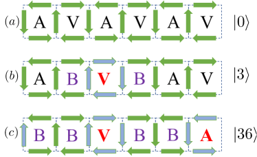
We are interested in the dynamics of the ladder plaquette, starting from a given initial configuration. A ladder with plaquettes (and periodic boundary conditions) contains spins, and hence presents in principle spin configurations, which would hence naively require qubits for its simulation. A more efficient procedure is possible, however, which we illustrate for the specific example of an RK-ladder with plaquettes initially prepared in an AVAVAV configuration. We denote this initial state as , which has obviously flippable plaquettes (see Fig. 2 (a)). Other initial states are possible, which will modify the specific mapping discussed below, but similar mappings may be found as well.
Flipping a plaquette blocks the two neighboring ones (see Figs. 2 (b) and (c)). For the mapping discussed below, it is crucial that in a ladder geometry, if flipping a plaquette blocks a neighboring one, the latter cannot be unblocked (i.e. transformed back into a flippable plaquette) by flipping a third one. Due to this key property, and if we are only interested in the flippable or non-flippable character of the plaquettes, we do not need to track why a plaquette is blocked. This is crucially different in a two-dimensional (2D) square lattice, where a blocked plaquette may be unblocked by flipping all the neighboring ones. As a result, in 2D geometries it is necessary to keep track why a plaquette is blocked, which results in a much more resource-consuming algorithm.
Due to the above-mentioned property, we may build the relevant states in a plaquette ladder by considering subsequent flips, without the need of describing the blocked plaquettes. We just need to keep track of which plaquettes have been flipped with respect to (denoted in bold red in the examples of Fig. 2 (b) and (c)), with the proviso that two neighboring plaquettes cannot be flipped. In the following, we employ the notation , which denote ladders in which plaquettes have been flipped with respect to the initial state . Figures 2 (b) and (c) show, respectively, the case of the states and . Successive application of flips results in different families of states. States within a given family can be obtained from each other by translation taking into account periodic boundary conditions.
For the case of plaquettes, the states with only one flip, , , have four remaining flippable plaquettes, see the example of Fig. 2 (b). Clearly these states form a single family. States with two flips split into two families: , with states with three flippable plaquettes, and , which have two flippable plaquettes. Finally, there are states with three flips , which have three flippable plaquettes each. Any other of the possible spin configurations of the ladder cannot be reached from , and hence does not need to be considered. The relevant Hilbert space fragment contains 18 states. However, the number of states taking part in the dynamics is significantly smaller, since flips only link to the symmetric superpositions of the states of each family:
| (8) | |||||
| (9) | |||||
| (10) | |||||
| (11) |
which form a closed set of states linked by the effective Hamiltonian , where
| (12) | |||||
| (13) | |||||
Note that the large reduction in complexity, from basis states to just five effective states for the case of -plaquette ladders, is based on the combination of gauge invariance, the above-mentioned property concerning blocked plaquettes, and symmetrization. This reduction of complexity allows for an efficient simulation of RK-ladders of a sizable number of plaquettes with a small number of qubits, well-suited for NISQ devices.
Simulations of larger number of plaquettes demand the construction, using a simple classical numerical procedure, of the families of states with different number of flips that are equivalent when applying translation under periodic boundary conditions. Each family contributes to one state of the effective basis, given by the symmetrization of all the states in the family. The number of effective states determines the number of equations , which demands the use of qubits. For larger , , hence reducing the number of necessary qubits by a factor of compared to the naive mapping of all spin states. For example, a sizable RK-ladder with plaquettes can be simulated, if noise is properly harnessed, with just qubits.

| Number of plaquettes | No. Pauli terms | No. CNOT (native) | No. CNOT (scaled) |
| 4 | 7 | 6 | 0 |
| 6 | 23 | 48 | 14 |
| 8 | 26 | 64 | 20 |
IV Quantum Simulation
We present below results for the dynamics of RK ladders with , , and plaquettes, which are described, respectively, by , and effective states, and which may be then evaluated using, respectively, , , and qubits (note that the simplest case with just two plaquettes, which we do not discuss, may be simulated with a single qubit). In order to simulate the dynamics with a quantum computer, we first decompose the effective Hamiltonian into a string of products of Pauli matrices , and , and the identity [29]. Table 1 provides the number of Pauli terms in the decomposition for different number of plaquettes in the RK ladder. For , the -qubit evaluation of the effective Hamiltonian in terms of Pauli terms acquires the form (for ):
| (14) | |||||
Expressing this linear superposition as , we may then evaluate the evolution operator using first order Trotter-Suzuki approximation [30, 31]
| (15) |
where , is number of Trotter steps and is the Trotter time step. In a standard quantum circuit implementation, each evolution operator is decomposed into single qubit rotations and CNOT gates [32, 33], as illustrated in the examples of Figs. 3 (a) and (b). However, in NISQ devices it is crucial to reduce as much as possible the number and duration of two-qubit operations, which constitute the main source of errors. Alternative implementations have been hence recently proposed [34, 35, 36], in which the use of scaled quantum gates allows to decrease the number of two-qubit operations, leading to a significant error reduction in the implementation.
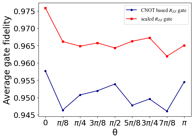
In IBM-Q machines, the CNOT operation is natively realized by the two-qubit rotation where Pauli and gates act on driven control and target qubits, respectively, implemented by echoed cross-resonance (CR) pulses [37]. A scaled can be implemented with CR pulses, where the rotation angle depends on the pulse area. This scaled is then used to implement a scaled as shown in Figs. 3 (c) and (d). Note that is central in the implementation of any interaction term of the effective Hamiltonian. Since errors mostly arise due to the CR pulses, the use of scaled to implement all the terms of the evolution operator reduces the overall error in the circuit by decreasing both the overall duration of the pulse schedule and the number of native CNOT gates in the circuit. Table 1 provides the number of native CNOT gates in the basis gate set implementation, and the number of remaining CNOT gates in the scaled gate implementation for plaquettes in one circuit repetition. Appendix A presents a detailed description of the generation of scaled gates and of the analysis of the average gate fidelity for the scaled implementation of against the standard CNOT implementation.
V Results
In order to evaluate the dynamics and benchmark the results obtained using a quantum device, we monitor two observables that characterize the dynamics in the RK ladder: the average number of flippable plaquettes , and the plaquette-plaquette correlations
| (16) |
Note that due to periodic boundary conditions, the correlation is independent of the particular choice of . The quantum simulation results discussed below were obtained using the noise model of the 7-qubit IBM-Q Lagos. In each simulation, we execute the quantum circuit for the unitary time evolution operator for Trotter steps with a given time step and measure counts with 8192 shots per measurement.
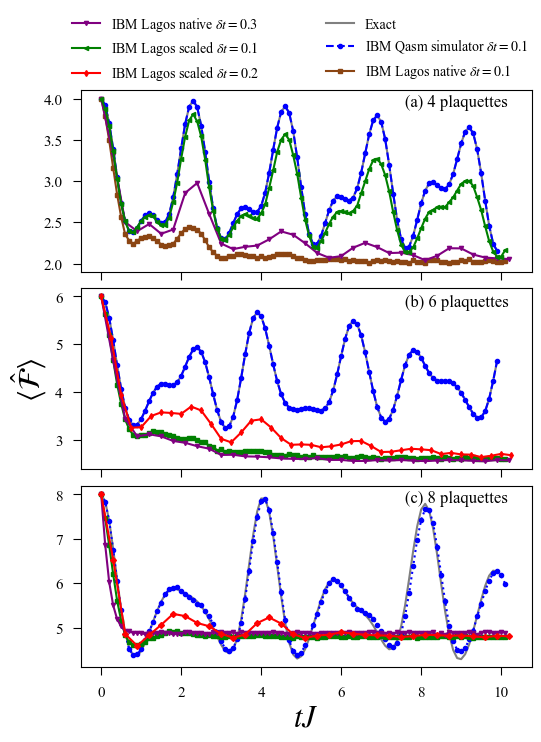
Figure 4 shows our results for and different number of plaquettes of up to a time . The figure compares our results using exact-diagonalization (ED, employing Krylov subspace), the ideal simulator, and the noisy circuit with non-scaled and scaled gates. As mentioned above, the minimal case of plaquettes can be solved with a single qubit, and as a result the two-plaquette quantum simulation in a noisy device matches exceptionally well with the ED calculations and ideal simulator calculations (not shown). The advantage of using scaled quantum gates becomes evident when considering the case of plaquettes. The simulation for a noisy device with scaled gates with a Trotter step is in very good agreement with the ideal simulation, giving significant improvement over the noisy quantum simulation with the native gates as seen in Fig. 4(a), which clearly fails already at .
For plaquettes, the number of CNOT gates is so large in the basis circuits that noisy quantum simulation with basis gates provides no useful data already for times . In contrast, we see from Fig. 4(b) that the quantum simulation using scaled gates for a Trotter step recovers the qualitative behaviour of the ideal quantum simulation, which matches well with the ED calculation. For plaquettes the Trotter error remains very small in the ideal simulation. Again the noisy basis circuit simulation fails to recover useful data for any , whereas the scaled gate simulation for a time step recovers the qualitative oscillation up to , see Fig. 4(c).
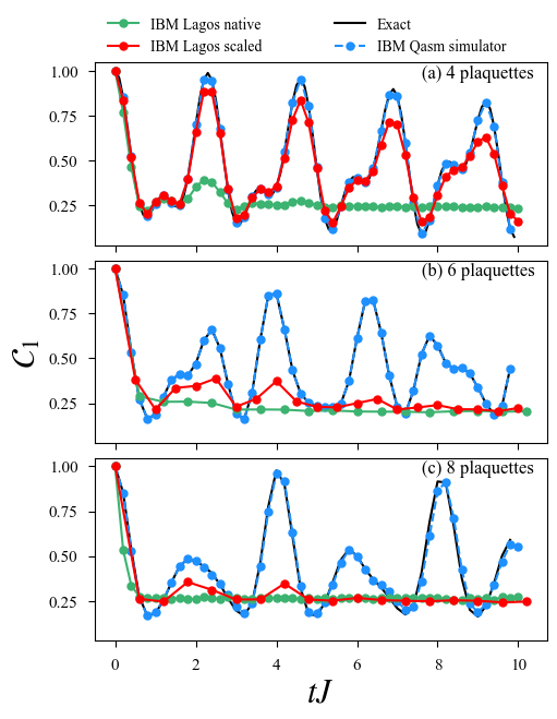
Figure 5 shows our results for the nearest neighbor correlation for RK-ladders with , and plaquettes. We compared again the ED results, the ideal quantum simulation, and the noisy quantum simulation with non-scaled and scaled gates, using for non-scaled gates and for scaled gates. These results show again that for noisy quantum simulations with re-scaled gates result in an excellent quantitative agreement with ED calculations, whereas those with basis gates fail already at short times . Moreover, we observe again that calculations with re-scaled gates provide a qualitatively correct behavior for for and , whereas the calculations with basis gates produce useless results already for .
VI Conclusions
We have shown that the dynamics of Rohksar-Kivelson ladders, a basic lattice gauge model, may be efficiently mapped into a small number of qubits due to the combination of gauge invariance, symmetrization, and the particular way plaquettes are blocked against ring-exchange. These properties reduce by a factor of the number of necessary qubits to simulate the dynamics of the RK ladder, an interesting feature for simulations in NISQ devices. We have illustrated the procedure using the simulator (including noise) of the 7-qubit IBM-Q machine Lagos, showing that the use of scaled gates allows for the faithful simulation of ladders of plaquettes. Moreover, we expect that using a combination of other error-mitigation techniques [26], in particular zero-noise extrapolation, should significantly improve the results for larger lattices, since even in this relative simple machine the qualitative behavior is well recovered at least up to for up to ring-exchange times.
Acknowledgements.
We acknowledge funding by the Volkswagen foundation and the Ministry of Science and Culture of Lower Saxony through Quantum Valley Lower Saxony Q1 (QVLS-Q1), and by the Deutsche Forschungsgemeinschaft (DFG, German Research Foundation) – under Germany’s Excellence Strategy – EXC-2123 Quantum-Frontiers – 390837967.References
- Georgescu et al. [2014] I. M. Georgescu, S. Ashhab, and F. Nori, Rev. Mod. Phys. 86, 153 (2014).
- Altman et al. [2021] E. Altman, K. R. Brown, G. Carleo, L. D. Carr, E. Demler, C. Chin, B. DeMarco, S. E. Economou, M. A. Eriksson, K.-M. C. Fu, M. Greiner, K. R. Hazzard, R. G. Hulet, A. J. Kollár, B. L. Lev, M. D. Lukin, R. Ma, X. Mi, S. Misra, C. Monroe, K. Murch, Z. Nazario, K.-K. Ni, A. C. Potter, P. Roushan, M. Saffman, M. Schleier-Smith, I. Siddiqi, R. Simmonds, M. Singh, I. Spielman, K. Temme, D. S. Weiss, J. Vučković, V. Vuletić, J. Ye, and M. Zwierlein, PRX Quantum 2, 017003 (2021).
- Bloch et al. [2012] I. Bloch, J. Dalibard, and S. Nascimbène, Nature Physics 8, 267 (2012).
- Kennes et al. [2021] D. M. Kennes, M. Claassen, L. Xian, A. Georges, A. J. Millis, J. Hone, C. R. Dean, D. N. Basov, A. N. Pasupathy, and A. Rubio, Nature Physics 17, 155 (2021).
- Cao et al. [2019] Y. Cao, J. Romero, J. P. Olson, M. Degroote, P. D. Johnson, M. Kieferová, I. D. Kivlichan, T. Menke, B. Peropadre, N. P. D. Sawaya, S. Sim, L. Veis, and A. Aspuru-Guzik, Chemical Reviews 119, 10856 (2019).
- Bauer et al. [2020] B. Bauer, S. Bravyi, M. Motta, and G. K.-L. Chan, Chemical Reviews 120, 12685 (2020).
- Bauer et al. [2023a] C. W. Bauer, Z. Davoudi, N. Klco, and M. J. Savage, Nature Reviews Physics 5, 420 (2023a).
- Bauer et al. [2023b] C. W. Bauer, Z. Davoudi, A. B. Balantekin, T. Bhattacharya, M. Carena, W. A. de Jong, P. Draper, A. El-Khadra, N. Gemelke, M. Hanada, D. Kharzeev, H. Lamm, Y.-Y. Li, J. Liu, M. Lukin, Y. Meurice, C. Monroe, B. Nachman, G. Pagano, J. Preskill, E. Rinaldi, A. Roggero, D. I. Santiago, M. J. Savage, I. Siddiqi, G. Siopsis, D. Van Zanten, N. Wiebe, Y. Yamauchi, K. Yeter-Aydeniz, and S. Zorzetti, PRX Quantum 4, 027001 (2023b).
- [9] U.-J. Wiese, Annalen der Physik 525, 777.
- Bañuls et al. [2020] M. C. Bañuls, R. Blatt, J. Catani, A. Celi, J. I. Cirac, M. Dalmonte, L. Fallani, K. Jansen, M. Lewenstein, S. Montangero, C. A. Muschik, B. Reznik, E. Rico, L. Tagliacozzo, K. Van Acoleyen, F. Verstraete, U.-J. Wiese, M. Wingate, J. Zakrzewski, and P. Zoller, The European Physical Journal D 74, 165 (2020).
- Aidelsburger et al. [2021] M. Aidelsburger, L. Barbiero, A. Bermudez, T. Chanda, A. Dauphin, D. González-Cuadra, P. R. Grzybowski, S. Hands, F. Jendrzejewski, J. Jünemann, G. Juzeliūnas, V. Kasper, A. Piga, S.-J. Ran, M. Rizzi, G. Sierra, L. Tagliacozzo, E. Tirrito, T. V. Zache, J. Zakrzewski, E. Zohar, and M. Lewenstein, Philosophical Transactions of the Royal Society A: Mathematical, Physical and Engineering Sciences, Philosophical Transactions of the Royal Society A: Mathematical, Physical and Engineering Sciences 380, 20210064 (2021).
- Chandrasekharan and Wiese [1997] S. Chandrasekharan and U.-J. Wiese, Nuclear Physics B 492, 455 (1997).
- Hauke et al. [2013] P. Hauke, D. Marcos, M. Dalmonte, and P. Zoller, Phys. Rev. X 3, 041018 (2013).
- Martinez et al. [2016] E. A. Martinez, C. A. Muschik, P. Schindler, D. Nigg, A. Erhard, M. Heyl, P. Hauke, M. Dalmonte, T. Monz, P. Zoller, and R. Blatt, Nature 534, 516 (2016).
- Klco et al. [2018] N. Klco, E. F. Dumitrescu, A. J. McCaskey, T. D. Morris, R. C. Pooser, M. Sanz, E. Solano, P. Lougovski, and M. J. Savage, Phys. Rev. A 98, 032331 (2018).
- Kokail et al. [2019] C. Kokail, C. Maier, R. van Bijnen, T. Brydges, M. K. Joshi, P. Jurcevic, C. A. Muschik, P. Silvi, R. Blatt, C. F. Roos, and P. Zoller, Nature 569, 355 (2019).
- Yang et al. [2020] B. Yang, H. Sun, R. Ott, H.-Y. Wang, T. V. Zache, J. C. Halimeh, Z.-S. Yuan, P. Hauke, and J.-W. Pan, Nature 587, 392 (2020).
- Nguyen et al. [2022] N. H. Nguyen, M. C. Tran, Y. Zhu, A. M. Green, C. H. Alderete, Z. Davoudi, and N. M. Linke, PRX Quantum 3, 020324 (2022).
- Kogut and Susskind [1975] J. Kogut and L. Susskind, Phys. Rev. D 11, 395 (1975).
- Moessner and Raman [2011] R. Moessner and K. S. Raman, Quantum dimer models, in Introduction to Frustrated Magnetism: Materials, Experiments, Theory, edited by C. Lacroix, P. Mendels, and F. Mila (Springer Berlin Heidelberg, Berlin, Heidelberg, 2011) pp. 437–479.
- Lewis and Woloshyn [2019] R. Lewis and R. M. Woloshyn, A qubit model for u(1) lattice gauge theory (2019), arXiv:1905.09789 [hep-lat] .
- Huffman et al. [2022] E. Huffman, M. García Vera, and D. Banerjee, Phys. Rev. D 106, 094502 (2022).
- Preskill [2018] J. Preskill, Quantum 2, 79 (2018).
- Cao et al. [2022] N. Cao, J. Lin, D. Kribs, Y.-T. Poon, B. Zeng, and R. Laflamme, Nisq: Error correction, mitigation, and noise simulation (2022), arXiv:2111.02345 [quant-ph] .
- Cai et al. [2023] Z. Cai, R. Babbush, S. C. Benjamin, S. Endo, W. J. Huggins, Y. Li, J. R. McClean, and T. E. O’Brien, Quantum error mitigation (2023), arXiv:2210.00921 [quant-ph] .
- Bharti et al. [2022] K. Bharti, A. Cervera-Lierta, T. H. Kyaw, T. Haug, S. Alperin-Lea, A. Anand, M. Degroote, H. Heimonen, J. S. Kottmann, T. Menke, W.-K. Mok, S. Sim, L.-C. Kwek, and A. Aspuru-Guzik, Rev. Mod. Phys. 94, 015004 (2022).
- Avkhadiev et al. [2020] A. Avkhadiev, P. E. Shanahan, and R. D. Young, Phys. Rev. Lett. 124, 080501 (2020).
- Rokhsar and Kivelson [1988] D. S. Rokhsar and S. A. Kivelson, Phys. Rev. Lett. 61, 2376 (1988).
- Hantzko et al. [2023] L. Hantzko, L. Binkowski, and S. Gupta, Tensorized pauli decomposition algorithm (2023), arXiv:2310.13421 [quant-ph] .
- Trotter [1959] H. Trotter, Proceedings of the American Mathematical Society 10, 545 (1959).
- Suzuki [1976] M. Suzuki, Communications in Mathematical Physics 51, 183 (1976).
- Nielsen and Chuang [2010] M. A. Nielsen and I. L. Chuang, Quantum Computation and Quantum Information: 10th Anniversary Edition (Cambridge University Press, 2010).
- Vatan and Williams [2004] F. Vatan and C. Williams, Phys. Rev. A 69, 032315 (2004).
- Earnest et al. [2021] N. Earnest, C. Tornow, and D. J. Egger, Phys. Rev. Res. 3, 043088 (2021).
- Stenger et al. [2021] J. P. T. Stenger, N. T. Bronn, D. J. Egger, and D. Pekker, Phys. Rev. Res. 3, 033171 (2021).
- Chen et al. [2022] I.-C. Chen, B. Burdick, Y. Yao, P. P. Orth, and T. Iadecola, Phys. Rev. Res. 4, 043027 (2022).
- Chow et al. [2011] J. M. Chow, A. D. Córcoles, J. M. Gambetta, C. Rigetti, B. R. Johnson, J. A. Smolin, J. R. Rozen, G. A. Keefe, M. B. Rothwell, M. B. Ketchen, and M. Steffen, Phys. Rev. Lett. 107, 080502 (2011).
- Alexander et al. [2020] T. Alexander, N. Kanazawa, D. J. Egger, L. Capelluto, C. J. Wood, A. Javadi-Abhari, and D. C. McKay, Quantum Science and Technology 5, 044006 (2020).
- Aleksandrowicz et al. [2019] G. Aleksandrowicz, T. Alexander, P. Barkoutsos, L. Bello, Y. Ben-Haim, D. Bucher, F. J. Cabrera-Hernández, J. Carballo-Franquis, A. Chen, C.-F. Chen, J. M. Chow, A. D. Córcoles-Gonzales, A. J. Cross, A. Cross, J. Cruz-Benito, C. Culver, S. D. L. P. González, E. D. L. Torre, D. Ding, E. Dumitrescu, I. Duran, P. Eendebak, M. Everitt, I. F. Sertage, A. Frisch, A. Fuhrer, J. Gambetta, B. G. Gago, J. Gomez-Mosquera, D. Greenberg, I. Hamamura, V. Havlicek, J. Hellmers, Łukasz Herok, H. Horii, S. Hu, T. Imamichi, T. Itoko, A. Javadi-Abhari, N. Kanazawa, A. Karazeev, K. Krsulich, P. Liu, Y. Luh, Y. Maeng, M. Marques, F. J. Martín-Fernández, D. T. McClure, D. McKay, S. Meesala, A. Mezzacapo, N. Moll, D. M. Rodríguez, G. Nannicini, P. Nation, P. Ollitrault, L. J. O’Riordan, H. Paik, J. Pérez, A. Phan, M. Pistoia, V. Prutyanov, M. Reuter, J. Rice, A. R. Davila, R. H. P. Rudy, M. Ryu, N. Sathaye, C. Schnabel, E. Schoute, K. Setia, Y. Shi, A. Silva, Y. Siraichi, S. Sivarajah, J. A. Smolin, M. Soeken, H. Takahashi, I. Tavernelli, C. Taylor, P. Taylour, K. Trabing, M. Treinish, W. Turner, D. Vogt-Lee, C. Vuillot, J. A. Wildstrom, J. Wilson, E. Winston, C. Wood, S. Wood, S. Wörner, I. Y. Akhalwaya, and C. Zoufal, Qiskit: An Open-source Framework for Quantum Computing (2019).
- Sheldon et al. [2016] S. Sheldon, E. Magesan, J. M. Chow, and J. M. Gambetta, Phys. Rev. A 93, 060302 (2016).
- Magesan and Gambetta [2020] E. Magesan and J. M. Gambetta, Phys. Rev. A 101, 052308 (2020).
- Sundaresan et al. [2020] N. Sundaresan, I. Lauer, E. Pritchett, E. Magesan, P. Jurcevic, and J. M. Gambetta, PRX Quantum 1, 020318 (2020).
- Kanazawa et al. [2023] N. Kanazawa, D. J. Egger, Y. Ben-Haim, H. Zhang, W. E. Shanks, G. Aleksandrowicz, and C. J. Wood, Journal of Open Source Software 8, 5329 (2023).
Appendix A Generation of scaled gates
In this section, we discuss the generation of scaled gates from a scaled gate using Qiskit Pulse [38, 39]. Since a longer pulse duration results in more error, can be scaled to a lesser pulse schedule duration and hence lesser two-qubit error than the CNOT based implementation of . The scaled is implemented by modifying the amplitude and duration of the gate , which generates the fundamental entangling operation for a CNOT gate, as outlined in Ref. [35, 36]. The is realized by echoed cross-resonance CR pulses and an -echoed -pulse applied on the control qubit. The -echoed -pulse serves to minimize the effect of and interaction terms [40, 41, 38]. Effects of other terms like and can be suppressed by applying certain rotary pulses [42]. A perfect gives rise to high fidelity entangling operation. The CR pulse has a Gaussian flat-top waveform, and has as attributes its flat-top width , its amplitude , its duration , and the number of standard deviations of Gaussian tails contained in the pulse . The area under the Gaussian pulse is then given by
| (17) |
To scale the pulse, depending on an arbitrary angle , the area under the CR Gaussian pulse is modified relative to the area of the CR pulse for such that the area under the modified pulse is given by
| (18) |
The modification in the pulse is achieved by either changing the width of the pulse or the amplitude, depending upon the initial parameters of the pulse. When , the pulse width is modified as
| (19) |
When , the flat-top width becomes 0 and we scale the amplitude as
| (20) |
We perform a simple Quantum Process Tomography experiment using qiskit-experiments library [43] to calculate the average gate fidelity for both the implementations of for various angles. We find that the scaled- has better fidelity than the CNOT-based implementation for all angles as shown in Fig. 6.
Appendix B Mapping for ladders with and plaquettes
Using the same notation as in the main text, the effective basis of states for the case of RK-ladders with plaquettes contains only states:
| (21) | ||||
Using these basis states, we can rewrite the effective Hamiltonian as
| (22) |
We map the Hamiltonian from states to an effective 3 states which can be simulated using 2 qubits.
For the case of plaquettes, the effective basis has states:
We define the basis states as
| (23) | ||||
Using these basis states, we can write the Hamiltonian in the form:
| (24) |
The corresponding dynamics can be then simulated using only three qubits.