Optimizing the method of images for regularized Stokeslets using theory and experiments of spheres moving near boundaries

Abstract

The general system of images for regularized Stokeslets (GSIRS) developed by Cortez and Varela (2015) is used extensively to model Stokes flow phenomena such as microorganisms swimming near a boundary. Our collaborative team uses dynamically similar scaled macroscopic experiments to test theories for forces and torques on spheres moving near a boundary, and use these data and the method of regularized Stokeslets (MRS) created by Cortez et al. (2015) to calibrate the GSIRS. We find excellent agreement between theory and experiments, which provides the first experimental validation of exact series solutions for spheres moving near an infinite plane boundary. We test two surface discretization methods commonly used in the literature: the six-patch method and the spherical centroidal Voronoi tessellation (SCVT) method. Our data show that the SCVT method provides the most accurate results when the motional symmetry is broken by the presence of a boundary. We use theory and the MRS to find optimal values for the regularization parameter in free space for a given surface discretization and show that the optimal regularization parameter values can be fit with simple formulae when using the SCVT method, so that other researchers have an easy reference. We also present a regularization function with higher order accuracy when compared with the regularization function previously introduced by Cortez et al. (2005). The simulated force and torque values compare very well with experiments and theory for a wide range of boundary distances. However, we find that for a fixed discretization of the sphere, the simulations lose accuracy when the gap between the edge of the sphere and the wall is smaller than the average distance between grid points in the SCVT discretization method. We also show an alternative method to calibrate the GSIRS to simulate sphere motion arbitrarily close to the boundary. Our computational parameters and methods along with our MATLAB and PYTHON implementations of the series solution of the Lee and Leal (1980) provide researchers with important resources to optimize the GSIRS and other numerical methods, so that they can efficiently and accurately simulate spheres moving near a boundary.

Background

The method of regularized Stokeslets [1] and the general system of images for regularized Stokeslets (GSIRS)[2] have been used extensively to model swimming microorganisms. The work of Shindell et al. (2021)[3] showed how dynamically similar macroscopic experiments and theory provide a principled method to calibrate the MRS and the GSIRS. Their model organism consisted of a cylinder and a helical flagellar filament with each body part calibrated separately using axial torque as a function of boundary distance. They showed that the optimal regularization parameter in the GSIRS simulations depended on the surface discretization, and they reported an optimal ratio of these two computational parameters. They also found that the optimal computational parameters depended strongly on the geometry of the object represented by the regularized Stokeslets. However, once the numerical model is precisely calibrated, forces and torques on a bacterium can be calculated with the GSIRS and swimming performance measures such as the Purcell efficiency [4], energy per distance [5, 6], and metabolic energy cost (energy per distance per body mass)[3] can be computed. Thus, accurate calibration of computational models allows determination of important structure function relationships when microorganisms are moving in their environment.

We use similar techniques in this work including theory and tank experiments to calibrate the GSIRS but consider spherical geometries, which may be used to model bacteria such as Rhodobacter sphaeroides and Enterococcus saccharolyticus and other organisms with spherical bodies [7, 8, 9]. The theoretical analysis of forces and torques on spheres moving near a boundary in Stokes flow has a long history beginning with the work of Jeffrey in 1915[10] who first found a series solution to the Stokes equations to calculate the torque on a sphere rotating with its axis perpendicular to an infinite plane. Subsequent work used similar techniques to find the drag on a sphere moving parallel to and perpendicular to a boundary[11, 12], and the torque on a sphere with its rotation axis oriented parallel to the boundary[13]. The linearity of the Stokes solutions allows any arbitrary motion of a sphere relative to a boundary to be decomposed into a sum of these four motions [14].

O’Neil and Bhatt (1991)[15] and Chaoui and Feuillebois (2002)[16] showed that previous series solutions, which require solving a truncated linear system to determine the coefficients of an infinite sum, could be replaced with a recursive method that minimizes computational cost to obtain the coefficients and solutions for the various types of motion. They showed that their method produces identical results at higher precision compared to numerical methods derived before. However, their solutions are only for a solid boundary, and their iterative scheme is not really necessary because solving these series solutions with 1000 terms is no longer computationally expensive.

Work by Lee and Leal (1980) [14] sought to unify various series solutions of sphere motion near a boundary into one linear system of equations that was able to calculate the force and torque for arbitrary motion near surfaces with varying properties. In their work, the parameter $\lambda$ represents the ratio of the viscosity of two fluids separated by an infinite surface. This parameter can also be thought of as the slip coefficient at the surface. A solid surface would therefore have a value of $\lambda=\infty$ (no slip) and a free surface a value of $\lambda=0$ (free slip).

While the Lee and Leal theory provide a theoretical basis to calculate the arbitrary motion of a sphere near a boundary, the four composite calculations have not been thoroughly verified with experiments [14]. Previous experimental work to verify theory has generally focused on either sedimentation experiments, such as those by Malysa and van de Ven (1986) [17], or on microscopic experiments[18, 19, 20, 21]. There have been some experimental tests of low Reynolds number torque on a sphere such as Maxworthy (1965)[22] and Kunesh et al. (1985)[23], but they studied a sphere in a rotating bath of liquid rather than a rotating sphere in a stationary tank. Thus, the experimental validity of the Lee and Leal theory is not known to high precision.

We test the theory using dynamically similar experiments in a cube-shaped tank that has dimensions about 50 times the radius of spheres. The increased drag due to the boundary is measured using high-precision sedimentation experiments, and high precision torque sensors are used to measure the increased torque due to the boundary on rotating spheres. We calculate the predicted influence of all six boundaries present in the tank experiment (five solid and one free surface and isolate the effects of a single finite boundary for comparison with the theory by subtracting the predicted force and torque from the other five boundaries. We are able to measure all four fundamental motions with respect to a no-slip plane wall: 1. increased drag from perpendicular translation 2. increased drag from parallel translation 3. increased torque from perpendicular rotation 4. increased torque from parallel rotation. Our experimental measurements provide the first comprehensive test of the theory and verify the accuracy of the Lee and Leal theory with much greater precision than previously reported. We provide numerical implementations of the Lee and Leal theory in user-friendly MATLAB and PYTHON GUI codes in the Supplemental Information.

The verified theory and our experiments provide us with reference values of forces and torques on a sphere moving near a solid boundary to precisely calibrate our numerical models, which use the GSIRS with different regularization functions and different methods of surface discretization. We present a new regularization function, $\psi_{\epsilon}$, that improves the order of accuracy of the results in the GSIRS over the commonly used $\phi_{\epsilon}$ developed in Cortez et al. (2005) [2], and we find optimal values of the regularization parameters by minimizing the percent error between simulations and theory for both regularization functions ($\psi_{\epsilon}$, $\phi_{\epsilon}$) in free space. We show that the spherical centroidal Voronoi tessellation (SCVT) discretization scheme, as developed by Du et al. (2003)[24], outperforms the six-patch discretization scheme because it distributes regularized Stokeslets more uniformly and is less sensitive to the orientation of the discretization to the boundary. Despite optimization in free space, we find that the GSIRS loses accuracy when the gap between the sphere and the boundary is smaller than the average distance between Stokeslets on the sphere. This result gives a general rule of thumb: the GSIRS may not be accurate within this distance and higher resolution (smaller distance between Stokeslets) is needed to ensure that the sphere is outside of the average distance between Stokeslets. Our library of experimental measurements and numerical implementations of theory are also reference values for other simulation schemes to aid other researchers in precisely calibrating their methods.

This article is organized as follows: Experimental Methods describes our dynamically similar experimental techniques to obtain the forces and torques for the four fundamental motions including removing finite size effects using the Lee and Leal theory. The Numerical Methods section describes our discretization and regularization schemes including the regularization function $\psi_{\epsilon}$ along with how we optimize the model using theory. In Results, we compare the experiments and optimized simulations to theory and discuss how to increase accuracy very near the boundary. The Discussion summarizes the performance of our calibrated model and our new empirical rule for establishing the minimum discretization needed for accuracy near a boundary.

Experimental Methods

Experiments were performed in a 225-liter tank (0.61 m $\times$ 0.61 m $\times$ 0.61 m) filled with approximately 180 liters of silicone oil (Clearco^® PSF-60,000cSt Polydimethylsiloxane). The fluid has a density of 970 kg/m³ and dynamic viscosity of $\mu=51.78\pm 0.32\rm\,Pa\cdot s$ at 25^∘ C, which is more than $10^{5}$ times the viscosity of water. The viscosity was measured using a Thermo Scientific rheometer (Haake Viscotester IQ). The fluid temperature was measured each day of experimental trials and the manufacturers temperature coefficient for the fluid ($1.00\times 10^{-6}$ kg/(m$\cdot$s)/^∘C) was used to adjust the viscosity value. The high viscosity fluid ensures that the Reynolds number was much less than unity in all experiments ($Re\approx 10^{-3}$) so that the incompressible Stokes equations (1) were valid for the typical length and speed scales in the experiments.

In all experimental tests of theory, we calculated the predicted contribution of all six boundaries in the tank (five solid and one free surface) and then subtracted any significant effects predicted by the Lee and Leal theory from the experimental data to isolate the effects on one boundary. Our rationale for this approach was to isolate the effect of one boundary on each type of motion, so that they could be compared to matching theoretical curves and numerical simulations, neither of which include such finite size effects. We are thereby able to test the utility of the theory in predicting the forces and torques on a sphere in a real-world experiment. The numerical implementation of theory is provided in the Supplementary Information for this article.

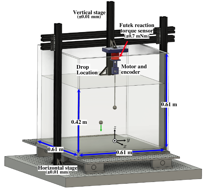
Figure 1: Sedimentation experiments: spheres were held in place using a neodymium magnet at the drop location. The 80-20 extruded aluminum had the same width as the sphere radius, so it was used to locate the sphere relative to the front vertical wall. A camera and tracking software measured the speed of the sphere as it fell under the influence of gravity. Torque experiments: schematic showing the tank, translation stage, torque sensor and a sphere positioned for measurement. The motor and magnetic encoder were housed inside a 3D-printed structure that was mounted to the active side of the torque sensor. Signal wires were run along the top of the 3D printed mounting structure and were secured in position for motor control and data acquisition.

Perpendicular and parallel translation

Fluid drag measurements were made by allowing spheres with radius $R=12.70\pm 0.03$ mm to sediment freely under the influence of gravity. They were released at a given distance from the boundaries using a piece of 80-20 extruded aluminum and a neodymium magnet to align them, see Fig. 1. The 80-20 stock had a corner bracket mounted with a screw aligned to the center of the 80-20 to which the magnet was attached and the sphere was held against the end of the screw beneath the fluid. The magnet was removed and the sphere fell, and because it was submerged, free surface effects were negligible.

We recorded motion tracking videos of falling spheres using a Point Grey GS3-U3-41C6M-C camera (2048 x 2048 pixels) and a Fujinon 25 mm focal length lens. For perpendicular drag measurements, the camera was positioned about 1 meter from the middle of the tank and aimed so that the bottom of the tank was approximately in the center of the field of view to minimize spherical aberration where the tracking required the most precision. For parallel drag measurements, the camera was positioned at the middle of the fluid column, so that it was aimed parallel to the boundary at the closest distance. The tank moved in the experiments, which ensured that the camera was well positioned for all parallel drag measurements. The manual aperture was also opened wide to create a more uniform focal plane. The frame rate was typically four FPS, which was sufficient to capture the slow motion of the spheres.

The fluid drag was calculated as the difference between the buoyant and gravitational forces, which were found using the mass and volume of the spheres: $F_{\rm net}=mg-\rho Vg$, where $m$ is the mass of the sphere, $g=9.8\rm\,m/s/s$ is the acceleration due to gravity, $V=4/3\pi R^{3}$ is the volume, and $\rho$ is the density of the silicone oil. The uncertainty in the gravitational and buoyant forces were very small and we considered them negligible.

The fluid drag forces in the $z-$dir, $F_{\perp}$ and $F_{\parallel}$, were made dimensionless by dividing by ($\mu Rv$), where $\mu$ is dynamic viscosity of the fluid, $R$ is the radius of the sphere, and $v$ is the instantaneous speed of the sphere. The speed was calculated using a central difference between the tracked positions divided by the time between frames.

The Lee and Leal theory predicts an additional drag of about 10% from the other five boundaries (four vertical and the upper free surface) in the location where perpendicular drag measurements were made, which was subtracted from the data. Our data for three trials are plotted with the theories by Lee and Leal along with the optimized MIRS simulations in Fig. 7a).

When measuring the perpendicular drag, we set $z=0$ as the bottom of the tank. We began tracking the spheres after they had fallen from the free surface to the middle of the fluid column to minimize the effect of the upper surface. They were then tracked until reaching the bottom boundary. Each track included a position and time, which was used to find the speed from the difference in their positions divided by the time between frames. The boundary distance, $d$, was calculated as the mean of the two $z-$direction positions used to calculated the speed. We present three trials in Fig. 7(a) showing very little scatter in the data, so we did not assign uncertainty for these data.

When measuring the parallel drag, we tracked the spheres for $\Delta z\approx 70$ mm after they were about $0.10$ m below the surface, where the additional drag from the upper and lower boundaries was approximately constant. We measured the boundary distance using the tracking video because the sphere experienced fluid forces towards the boundary along with adhesive forces at the release point that changed its distance to boundary by about $0.2$ mm. Uncertainty for these data were calculated by assigning an uncertainty of $\Delta z=\pm 0.035$mm based on the variance in measurements of the diameter of the sphere between frames in the video data and using standard error propagation. The uncertainty in the speed was typically $\Delta v\approx 0.3$ mm/s.

We ignored any rotational effects caused by the small net torque that results from the larger drag on the side of the sphere closest to the boundary. The Lee and Leal theory does predict that a small force on a rotating sphere directed towards the boundary, but the predicted torque from theory is very small, so the resulting rotation would be equally small. We marked the spheres and did not see any appreciable rotation even at the closest boundary distances.

Perpendicular and parallel rotation

Torque measurements used a Bal-Tec^® ball gauge that consists of a stainless steel sphere of radius $R=12.70\pm 0.01$ mm with a precision hole drilled along a diameter. We removed the manufacturer’s supplied shaft and attached a carbon steel rod with radius $r=4.763\pm 0.013$ mm and length $L=304.8\pm 0.1$mm. The rod was attached via a shaft adapter to a DC motor with an inbuilt magnetic encoder (Pololu 4846), which was mounted inside of a custom 3D-printed enclosure. The shaft passed through a sleeve bearing to minimize frictional torque and to keep the shaft aligned. Precession of the sphere when rotating was $<0.25$mm.

The rod+sphere assembly was located in the middle of the tank so that the four vertical walls were equidistant, as shown in Fig. 1. The distance to the bottom boundary was adjusted using a vertical stage under computer control with a resolution $\pm 0.01$mm. The tank was filled with silicone oil to a depth of 0.27 m, so that the bottom boundary could be touched by the lower edge of the sphere without immersing the torque sensor. The location where the sphere touched the bottom boundary was found by inspection using a laser pointer to help identify any small gaps. Once the zero point was established, the stage could reliably position the sphere with respect to the bottom boundary.

The DC motor was controlled using an ARDUINO MEGA 2560 with an ADAFRUIT Motor Shield v.2 attached. The motor encoder output was read using an Agilent 53132A Frequency counter and connected to the computer via a USB to GPIB connector (NI GPIB-USB-HS). The Agilent counter removed high frequency noise using the counter’s hardware-based 100kHz low pass filter. The GPIB read rate was about 1.5 samples per second.

A FUTEK TFF400, 10 in-oz, Reaction Torque Sensor measured the torque, and a FUTEK Amplifier Model IAA100 amplified the signal. The amplifier output was fed into a National Instruments (NI USB-6211) data acquisition board’s analog to digital input with a resolution of 250 thousand samples per second, but data acquisition was slowed to about ten samples per second because of the read rate of the computer.

We recorded data at varying rotational speeds and recorded the motor encoder data at the same time. We compensated for the different read rates of these data (frequency at 1.5/s and torque at 10/s) using a time stamp to interpolate frequency data to the same time points where torque samples were recorded, see Fig. 2. This interpolation was necessary so that we could non-dimensionalize the torque using the quantity $(\mu\Omega R^{3})$, where $\mu$ is the dynamic viscosity, $\Omega$ is the angular speed of the rotating sphere, and $R$ is the sphere radius. Dimensionless quantities were used for easy comparison with theory and simulations.

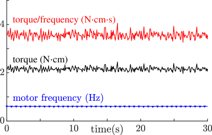
Figure 2: Example of torque and frequency signals from the experimental torque measurements. The frequency (solid blue symbols) was read with an Agilent counter via GPIB at about 1.5 samples per second with a 150 kHz low-pass filter, and torque data (solid black curve) were read using a DAQ at about 10 samples per second. The frequency data were interpolated to the the same time points that torque data were collected (solid blue curve), so that the torque per unit frequency could be calculated (solid red curve), which allowed the torque to be expressed as a dimensionless quantity for comparison to theory and simulations.

We took data for about 80 rotation periods (typically 60-80s) in both the CW and CCW rotation directions at each boundary location. An analysis script read the data files and used the mean of CW and CCW as the value at that boundary distance and the difference between CW and CCW torque values, which should have been the same, as the uncertainty in the experimental measurements. The value of $\tau_{\perp}$ for the sphere was found by subtracting the torque from the cylinder holding the sphere.

We used the theory of Jeffrey and Onishi [25], which was previously confirmed by Shindell et al. [3], to calculate the torque on the length of the rod inserted into fluid and subtract it from the overall torque signal. The computed cylinder torque was typically $\approx 10\%$ of the total signal. We ignored any possible effects from the interaction of the flow fields induced by the cylinder and sphere. Unlike for the drag measurements, the theory predicts a negligible contribution to the torque from finite size effects($<0.1\%$) at these distance to the other five boundaries, so they were also ignored. A plot of the dimensionless torque versus scaled boundary distance is shown in Fig. 8(a) along with the theory and simulations.

We used the same methods to measure the torque for rotation with the axis parallel to the wall except that the tank was filled to a depth of 0.42 m and the sphere was held at a fixed depth of 0.21 m. The horizontal stage with the same resolution ($\pm 0.01$mm) as the vertical stage was used to locate one of the vertical walls near the sphere, as shown in Fig. 1. Here again, finite size effects of from the other five boundaries were considered negligible. Parallel axis rotation torque data is shown in Fig. 8(b) and plotted in the same manner as the perpendicular axis rotation data.

Numerical methods

A primary goal of our work is to develop an optimized method of modeling spheres moving near a boundary. We use the experimentally tested theory of Lee and Leal [14] to provide reference values for the optimization. Any numerical simulation of a solid object moving in a fluid has two inherent types of error: those from approximations in the method and those from discretizing the solid object. To improve the accuracy in the model and the performance of the GSIRS [1], we first introduce a combination of a high-order regularization function and a surface discretization with uniform point distribution. Then we find optimal values for the regularization parameter in free space and near a boundary. We investigate two discretization methods commonly used in the literature – the six-patch method and the spherical centroidal Voronoi tessellation (SCVT) method to understand how the percent error relative to theory is affected by the number of grid points and the orientation of the discretized points relative to the boundary for each type of discretization. We then simulate sphere motion near a boundary for a large range of boundary distances and compare the results with experiments and theory.

Regularization function

The MRS developed by Cortez et al. (2005) [2] uses a regularization function to replace singular point forces arranged on a surface that represents a solid object in Stokes flow. Replacing the singular forcing with a regularization function (a radially smooth approximation of the Dirac delta distribution) creates a linear system of equations that can be solved without using specialized methods to accommodate the singularities. The GSIRS extends the MRS to include a solid boundary by imposing a counter Stokeslet, a potential dipole, a Stokeslet doublet, and two rotlets at the image point of each discrete point $\mathbf{x}_{k}$. The image system thereby imposes a no-slip condition by canceling the fluid velocity at the boundary, as shown in [1]. We use the MRS and GSIRS in our work by prescribing velocities on the discretized sphere and solving the regularized system to calculate the net force and net torque acting on the sphere. We use the GSIRS to simulate each of the four fundamental motions of a sphere near an infinite planar surface: perpendicular translation, parallel translation, perpendicular axis rotation, and parallel axis rotation [14].

The simulations solve the incompressible Stokes equations with external forcing:

$$\mu\triangle\mathbf{u(\mathbf{x})}-\nabla p(\mathbf{x}) =-\mathbf{F(\mathbf{x})}\text{ and}$$ (1)

$$\nabla\cdot\mathbf{u(\mathbf{x})} =0,$$

where $\mathbf{u}$ is the fluid velocity, $p$ is the fluid pressure, and $\mu$ is the dynamic viscosity. The vector $\mathbf{F}$ is the sum of the force density applied at discrete points $\mathbf{x}_{k}$, $k=1,...,N$ on the sphere model, i.e., $\mathbf{F}(\mathbf{x})=\displaystyle\sum_{k=1}^{N}\mathbf{f}_{k}\omega_{\epsilon}(\mathbf{x}-\mathbf{x}_{k})$ where $\mathbf{f}_{k}$ is a point force at $\mathbf{x}_{k}$ and $\omega_{\epsilon}(\mathbf{x})$ is a regularization function having an integral equal to unity over $\mbox{\bf R}^{3}$.

Given a point force at $\mathbf{x}_{0}$, the MRS derived for an arbitrary regularization function, $\omega_{\epsilon}(r)$ where $r=|\mathbf{x}-\mathbf{x}_{0}|$ is written in terms of the functions $\mbox{$G_{\epsilon}$}(r)$ and $\mbox{$B_{\epsilon}$}(r)$, which satisfy $\Delta\mbox{$G_{\epsilon}$}=\omega_{\epsilon}$ and $\Delta\mbox{$B_{\epsilon}$}=\mbox{$G_{\epsilon}$}$. In the far field, these functions approach their singular counterparts $G_{0}(r)=-(4\pi r)^{-1}$ and $B_{0}(r)=-(8\pi)^{-1}r$. The far field error can be controlled by constructing a regularization function that produces rapid convergence of the regularized Stokeslet to the singular one. The convolution of the regularization function $\omega_{\epsilon}(\mbox{\bf x})$ with a smooth function $f(\mbox{\bf x})$ can be a high-order approximation of $f(\mbox{\bf x})$ by forcing the regularization function to satisfy certain moment conditions. Nguyen et al. [26] show that the convergence rates of these approximations are directly related to the decay rate of $\omega_{\epsilon}(r)$ when the following moment conditions are satisfied:

$$\int_{0}^{\infty}r^{2}\omega_{\epsilon}(r)dr = (4\pi)^{-1}$$ (2)

$$\int_{0}^{\infty}r^{4}\omega_{\epsilon}(r)dr = 0.$$ (3)

Nguyen et al.[26] also established that if $\omega_{\epsilon}(r)$ does not satisfy condition (3), then $|\mbox{$B_{\epsilon}$}(r)-B_{0}(r)|=O(r^{-2})$ for $\epsilon\ll r$ regardless of the decay properties of $\omega_{\epsilon}(r)$.

In our work, we choose $\omega_{\epsilon}(r)$ as:

$$\phi_{\epsilon}(r)=\frac{15\epsilon^{4}}{8\pi(r^{2}+\epsilon^{2})^{7/2}}\\ \qquad\text{or}\qquad\psi_{\epsilon}(r)=\frac{15\epsilon^{4}(40\epsilon^{6}-132\epsilon^{4}r^{2}+57\epsilon^{2}r^{4}-2r^{6})}{16\pi(r^{2}+\epsilon^{2})^{13/2}},$$

where $r=|\mathbf{x}-\mathbf{x}_{k}|$ and $\epsilon$ represents the regularization parameter. Two-dimensional plots of $\phi_{\epsilon}(r)$ and $\psi_{\epsilon}(r)$ are shown in Fig. 3(a), for reference.

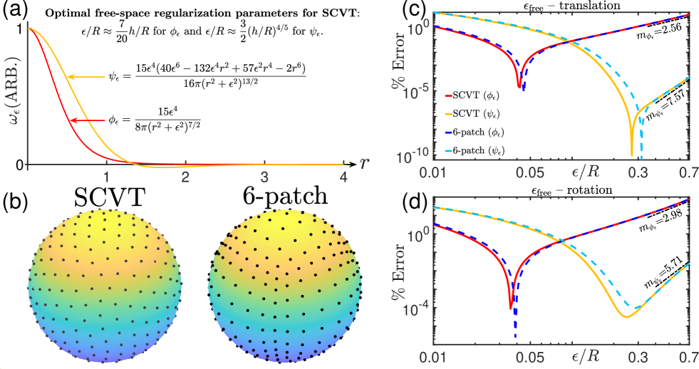
Figure 3: Finding optimal regularization parameters in free space: (a) Regularization functions $\phi_{\epsilon}$ and $\psi_{\epsilon}$ are normalized such that their values at the center are equal; (b) Surface discretizations ($N$ = 296) on a sphere using SCVT and 6-patch show that the point distribution is more uniform for SCVT. The average distance between discretization points for the SCVT discretization scheme is defined as $\displaystyle h=\sqrt{\frac{4\pi R^{2}}{N}}$. Optimal regularization parameters for (c) translation and (d) rotation in free space with $N=1000$ (SCVT) and $N$ = 1016 (six patch): the minima of the percent errors for the four different combinations are used to identify the value of the optimal regularization parameters. For SCVT, the optimal regularization parameter $\epsilon$ for each regularization function can be estimated as a function of value of $h$, see Fig 4. The decay properties of the regularization functions $\phi_{\epsilon}$ and $\psi_{\epsilon}$ are shown as dash-dot lines that represent the slope of the best fit line used to determine the exponent $m$ in Eq. (4) as $\epsilon\to\infty$.

The sphere motion we simulate generates forces distributed over surfaces of solid objects rather than volumes, so the conditions that reduce the regularization error are different. The velocity field at any location is given by the surface integral of the Stokeslet, $\displaystyle\int_{\Gamma}S(\mbox{\bf x},\mbox{\bf y}(A))\mbox{\bf f}(A)dA$. Approximating this integral by a quadrature and replacing the Stokeslet with a regularized Stokeslet, $\displaystyle\sum_{k=1}^{N}S_{\epsilon}(\mbox{\bf x},\mbox{\bf y}_{k})\mbox{\bf f}_{k}\Delta A_{k}$ creates two types of error: one from the discretization of the integral and the other from the regularization of the Stokeslet. The form of the total error is important to establish convergence of the method. The total error is given by:

$$Err(\mbox{\bf x})=O\left(\frac{h^{p}}{\epsilon^{q}}\right)+O(\epsilon^{m}),$$ (4)

where $h$ is the discretization length and the exponents $p$, $q$, and $m$ depend on the specific implementation of the numerical method used to compute the surface integrals [2, 27, 28]. The first term is the discretization error, and its form depends on the regularization function used, the quadrature method, and whether periodicity can be exploited. Our work focuses on the second term, the regularization error, which depends only on the regularization function. Equation (4) implies that the regularization error dominates when $\epsilon$ is large compared to $h$, which we exploit when analyzing the two regularization functions, see Fig. 3.

Beale [29] showed that for surface forces in water waves, the following additional constraint on $\epsilon$ reduces the regularization error by increasing the exponent $m$ in (4):

$$\int_{0}^{\infty}(-4\pi r\mbox{$G_{\epsilon}$}(r)-1)r^{2k}dr=0,\ \ \ \textrm{ for }k=0,1,2,\dots$$ (5)

The regularization function $\omega_{\epsilon}=\mbox{$\phi_{\epsilon}$}(r)$ satisfies only criterion (2), whereas our regularization function $\omega_{\epsilon}=\psi_{\epsilon}(r)$ satisfies (2)-(3) and (5) for $k=0$ and $1$.

Figure 3 (a) shows plots of the regularization functions $\phi_{\epsilon}$ and $\psi_{\epsilon}$ arbitrarily scaled so that they have the same maximum value and their functional forms can be more easily compared. The function $\phi_{\epsilon}$ is positive for all $r$, but the function $\psi_{\epsilon}$ must have positive and negative values in order to satisfy the moment conditions in Eq. (5). Since both functions have integral equal to one, $\psi_{\epsilon}$ must be wider in the positive region to compensate for the negative contribution to the integral, which is reflected in the size of optimal regularization parameter found in the next section.

Sphere discretization

We analyze two methods for discretizing a sphere: the six-patch and the spherical centroidal Voronoi tessellation (SCVT), as shown in Figure 3(b). The six-patch method distributes points from a bounding cube to the sphere’s surface[30, 2, 27, 31]. The number of points is determined using the formula $N=6n^{2}-12n+8$, where $n$ is the number of points on each edge of the cube. While, the six-patch method is commonly used and is easy to implement, the point distribution is not uniform on the sphere’s surface and can lead to errors in the simulation.

Our SCVT simulations used the method developed by Du et al. (2003)[24], which produces a nearly uniform point distribution on the sphere. This method implements the iterative process of moving the generating point of each Voronoi cell to its constrained mass centroid on the sphere until a convergence criterion is met. The resulting set of points is a local minimization of a cost function that represents the distortion of the generating points from their mass centroids with respect to a user-specified density function. We used the SCVT software available at Lili Ju’s website [32] with a constant density function to distribute the points as uniformly as possible on the surface. Figure 3 (b) compares the uniformity of the point distributions when using the SCVT and 6-patch methods for $N=296$ points. These two discretization methods allowed us to investigate how point uniformity affects the accuracy of our simulations for sphere motion near a boundary. Fig. 3(c)-(d) show the percent errors relative to theory for a translating sphere and a rotating sphere in free space computed using the MRS for both discretization types.

Optimal regularization parameter

We used the Stokes flow values of drag and torque on a sphere, $6\pi\mu RU$, and $8\pi\mu R^{3}\Omega$, respectively to optimize the value of a regularization parameter, $\epsilon$, in the MRS to simulate the drag for a translating sphere and the torque for a rotating sphere in free space. We incremented the regularization parameters from $\epsilon/R=0.01$ to 0.7 in steps of 0.001 for each motion, each type of regularization function, and each discretization method. The range of simulation parameters used are reported in Table 1. We then computed the percent errors between the simulations and theory versus regularization parameter size for each motion, see for example Fig. 3(c)-(d). Overall, 55,280 calculations were conducted: two motion types (translation and rotation), two regularization functions ($\phi_{\epsilon}$, $\psi_{\epsilon}$), two discretization methods (SCVT, 6-patch), 10 values of $N$, and 691 values of regularization parameters, $\epsilon$.

Figures 3(c)-(d) show that for each value of $N$ there is an optimal value of $\epsilon$ corresponding to each combination of regularization function and discretization that minimizes the percent error when compared to theory of each motion. In addition to reporting these optimal values of the regularization parameters in free space, we discuss other options for optimizing the regularization parameters near a boundary in Results, below.

Simulation summary

We used three sets of simulations to minimize the error relative to theory when simulating the sphere motions we studied in our experiments. The first set of simulations used the MRS to understand which regularization function, $\phi_{\epsilon}$ or $\psi_{\epsilon}$, converges most rapidly as the regularization parameter size increases. These simulations were also used to find an optimal value for the regularization parameter $\epsilon$ for each combination of the regularization function and discretization method. The second set of simulations used GSIRS and the optimal regularization parameters from the first set of simulations to assess how orientation relative to the boundary of the six-patch and SCVT discretizations affects the percent error when compared to theory. We then simulated sphere motion for a large range of boundary distances using our free-space-optimized regularization parameters, SCVT, and the high-order regularization function $\psi_{\epsilon}$ for comparison with the experiments and theory. For the last set of simulations, we further explored how to optimize values for the regularization parameter at very small boundary distances for the sphere motions.

Table 1: Parameters values used in numerical simulations.

Parameter	Value
Dynamic viscosity	$\mu=10^{-3}\,\rm{Pa\cdot s}$
Sphere radius	$R=1\mu\rm{m}$
Translation speed	$U=1\mu\rm{m}/s$
Rotation rate	$\Omega/(2\pi)=154\,\rm{Hz}$
Discretization #	$N$(six-patch) $\in\{98,152,218,296,$
	$386,488,602,728,866,1016\}$
	$N$(SCVT) $\in$ {100:100:2400}

Results

Comparison of experiments with theory

Figures 7 and 8 show that the theory of Lee and Leal [14] worked very well within experimental uncertainty to remove the finite size effects in an experiment, where the tank is approximately $48R\times 48R\times 30R$, where $R=12.70\pm 0.03$mm. Our tank was large enough that the predicted increased torque was less than the experimental uncertainty and was ignored. However, the theory predicts a significant increase in the drag on a sedimenting sphere $(\sim 10\%)$ even in the middle of the tank. The other finite size effects such as corners, free surface motion, etc. are small enough that the Lee and Leal theory for an infinite smooth plane is useful for predicting the influence of both solid and free surfaces in a tank experiment, at least for a tank of the size we used. Our experimental measurements provide a level of precision unmatched by previous experimental tests of theory.

Optimizing the MRS and GSIRS

Comparison of regularization functions

We used the plots of percent error versus regularization parameter size to assess the order of accuracy of each regularization function based on Eq. (4). Figure 3(c)-(d) shows an example of finding the exponent $m$ in Eq. (4) from a log-log plot of percent error versus regularization parameter, $\epsilon$. Using the regularization function, $\psi_{\epsilon}$ instead of $\phi_{\epsilon}$ increases the value of from $m=$ 2.56 to $m=$ 7.57 in the translation data and increases $m$ from 2.98 to 5.71 in the rotation data, where the number of discretization points is about the same for all data with $N_{\text{six-patch}}=1016$ and $N_{\rm SCVT}=1000$. Thus, $\psi_{\epsilon}$ shows a higher order of accuracy than $\phi_{\epsilon}$  which we attribute to the former satisfying the higher moment conditions, as described in Numerical Methods above.

These plots also allowed us to find the optimal regularization parameters for each type of motion and each combination of discretization method and regularization function. The value of $\epsilon$ that minimizes the percent error was easily identifiable, as shown in Fig. 3(c)-(d).

We report the optimal regularization parameters in free space in Fig. 4 for SCVT. The optimal value of $\epsilon$ varies smoothly as a function of the average discretization size $\displaystyle h=\sqrt{\frac{4\pi R^{2}}{N}}$, so we found fit functions that relate $\epsilon$ and $h$ for each of the regularization functions:

$$\epsilon_{\rm est}/R \approx\frac{7}{20}h/R\quad\text{ for }\phi_{\epsilon}$$ (6)

and

$$\epsilon_{\rm est}/R \approx\frac{3}{2}(h/R)^{\frac{4}{5}}\quad\text{for }\psi_{\epsilon}.$$ (7)

These formulae allow other researchers to bypass the free-space-optimization process and use the fit functions to find the optimal value of $\epsilon$. The six-patch data did not allow such formulas to be found because the discretization length is not uniform. We note that the value of $\displaystyle\epsilon_{\rm est}/R$ for $\phi_{\epsilon}$ is very different than the value found for cylinders by Shindell et al. (2021)[3]. In their work, they found that $\epsilon/R=(h/R)/6.4$, where $h$ was the discretization length between Stokeslets on a side surface of a cylinder. Thus, we confirm the result of Shindell et al. that the relationship between discretization length $h$ and the optimal regularization size $\epsilon$ depends on the geometry of the solid object being simulated.

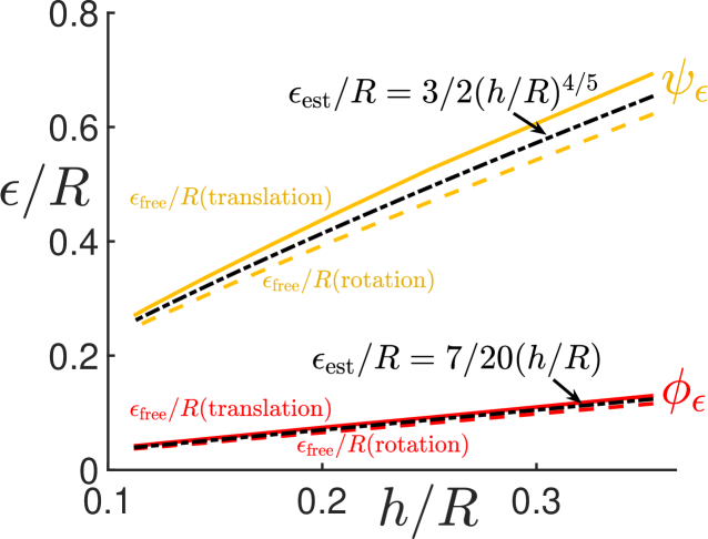
Figure 4: Optimal regularization parameters in free space for SCVT for different surface discretizations with average discretization lengths, $\displaystyle h=\sqrt{\frac{4\pi R^{2}}{N}}$, where $N$ is the number of grid points and $R$ is the sphere radius. The optimal regularization parameter, $\epsilon_{\rm free}/R$, for each regularization function can be estimated as a function of the average SCVT discretization length, $\displaystyle h$, for both types of sphere motion. The fit function estimates for the regularization parameters are shown as black dash-dot curves. The relative difference between optimal regularization parameter for rotation and translation is approximately the same for $\psi_{\epsilon}$ and $\phi_{\epsilon}$, but is exaggerated for $\psi_{\epsilon}$ because of the scale in the plot. The mean of the ratio (rotation to translation) of the optimal regularization parameters is 0.91$\pm$0.01 for $\psi_{\epsilon}$ and 0.88$\pm$ 0.01 for $\phi_{\epsilon}$.

Comparison of discretization methods

We used the GSIRS, the two regularization functions $\phi_{\epsilon}$ and $\psi_{\epsilon}$, and the free-space-optimized regularization parameters found in the first set of simulations to simulate drags and torques for the four motions: perpendicular translation, parallel translation, perpendicular axis rotation, and parallel axis rotation. We used a range of discretization points $100\leq N\leq 1016$, and we broke any symmetry of the discretization with respect to the boundary by rotating the surface discretization along a random axis and by a random angle in each simulation. We evaluate the performance of each discretization method near the boundary because they are all optimized to perform well far from the boundary. Figure 5 shows the mean percent error versus number of grid points at three small boundary distances: $d/R$ = 1.089, 1.128, 3.0. There were 17,280 calculations in total: four motions, two regularization functions, two discretization methods, 10 values of $N$, three distances, and 36 random trials.

Generally, the percent error decreases as $N$ increases, as expected, but the rate at which this occurs is different. Simulations using $\psi_{\epsilon}$ (solid gold and dashed cyan curves) show a more rapid decrease in percent error as $N$ increases when compared to matched simulations using $\phi_{\epsilon}$ (solid red and dashed dark blue curves). The data also show that SCVT simulations using either regularization function (solid gold and solid red curves) generally return a lower mean percent error than the matched six-patch simulations (dashed cyan and dashed dark blue curves) especially when $N\approx$ 1000.

However, we note that the simulations for the closest boundary distance $d/R=$ 1.089 shown in Fig. 5 (a)-(d) show large variance and large percent errors even at the highest resolution for all simulation types. Table 2 lists the range of the percent errors for these simulations when $800\leq N\leq 1016$: the performance is especially poor for the translational motion perpendicular to the wall as seen in Fig. 5 (c).

Table 2: Range of percent errors for $d/R=1.089$ and $800\leq N\leq 1016$ for four motions. The range was determined by finding the smallest (min) and largest (max) percent errors of each combination of the discretization method (SCVT or 6-patch) and the regularization function ($\phi_{\epsilon}$ or $\psi_{\epsilon}$) for all these values of $N$.

min - max	SCVT ($\phi_{\epsilon}$)	SCVT ($\psi_{\epsilon}$)	6-patch ($\phi_{\epsilon}$)	6-patch ($\psi_{\epsilon}$)
$F_{\parallel,\text{trans.}}$	2.604 - 2.911	1.643 - 1.888	1.635 - 3.940	1.837 - 3.256
$\tau_{\parallel,\text{rot.}}$	1.837 - 2.213	0.113 - 0.307	1.076 - 2.818	0.004 - 1.453
$F_{\perp,\text{trans.}}$	36.167 - 38.847	17.761 - 36.160	24.117 - 46.052	35.575 - 231.592
$\tau_{\perp,\text{rot.}}$	0.023 - 0.076	0.007 - 0.018	0.005 - 0.137	0.0269 - 0.064

Further from the boundary when $d/R=1.128$, as shown in Fig. 5 (e) - (h), the data are easier to interpret. The percent errors are reduced typically by an order of magnitude and the variance is much lower, but the SCVT simulations using $\psi_{\epsilon}$ generally converge more quickly, have lower variance, and achieve lower percent error at the highest value of $N$, as shown in panels (e) - (g), though there is no clearly superior method for simulating the perpendicular torque shown in panel (h). Once the distance is $d/R=3$ the six-patch and SCVT show similar performance in mean percent error values, which are small for all simulation types.

We extended our analysis of the variance in the different simulation types by plotting the relative standard deviation (RSD) of the mean value of force and torque, as shown in Fig. 6. The plots of RSD versus number of grid points $N$ show that the SCVT simulations are much less sensitive to the orientation of the sphere with respect to the boundary at any boundary distance. In general, the SCVT simulations outperform the six-patch method because the latter are still sensitive to the orientation of the discretization with respect to the boundary. In Fig. 6(c), the six-patch simulations show an RSD as high as 90% for the perpendicular translation data while the SCVT has an RSD of 1-2%. The asymmetry of the six-patch discretizations method therefore requires care to ensure the discretization does not skew results near the boundary and requires averaging of different orientations for accuracy, whereas the SCVT shows very little variance in the computed force or torque. Thus, averaging over 36 orientations when using an SCVT discretization, as we have done for analysis, is not necessary.

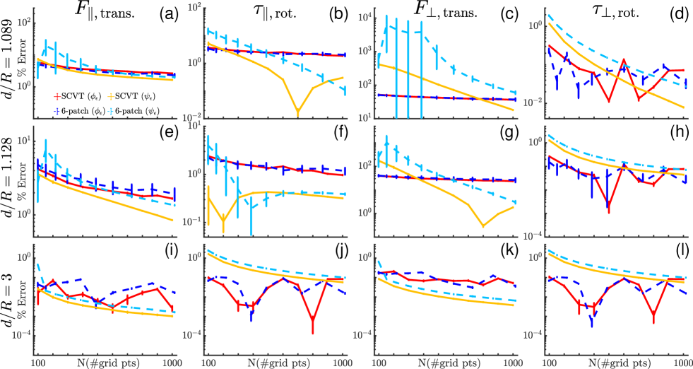
Figure 5: The figures show percent errors for the four fundamental sphere motions relative to theory versus number of discretization points, $N$, at three locations near a boundary: $d/R=1.089$ (top row), $d/R=1.128$ (middle row), and $d/R=3$ (bottom row): (a), (e), and (i) are drag when moving parallel to the boundary, (b), (f), and (j) are torque with the rotation axis parallel to the boundary, (c), (g), and (k) are drag when moving perpendicular to the boundary, and (d), (h), and (l) are torque with the rotation axis perpendicular to the boundary. Solid lines are simulations that used the SCVT discretization and dashed lines show data using the six-patch discretization. Red and dark blue curves are simulations that used the $\phi_{\epsilon}$ regularization function, whereas the cyan and gold curves used the new $\psi_{\epsilon}$ regularization function. Each sphere motion was simulated 36 times with the sphere’s discretization rotated along a random axis and a random angle to analyze the effects of sphere orientation on the accuracy the computation. The percent error is the mean of the 36 random trials, and the error bars are the standard deviation of the trials. The SCVT simulations show a much lower variance when compared with the six-patch simulations (see Fig. 6), and the SCVT generally show smaller percent errors at the highest values of $N$. The top row shows that once the gap between the edge of the sphere and the boundary, $d/R-1=0.089$, is smaller than a discretization length, $h/R\in[0.11,0.35]$ for $98\leq N\leq 1016$, the percent error and the variance are much higher.

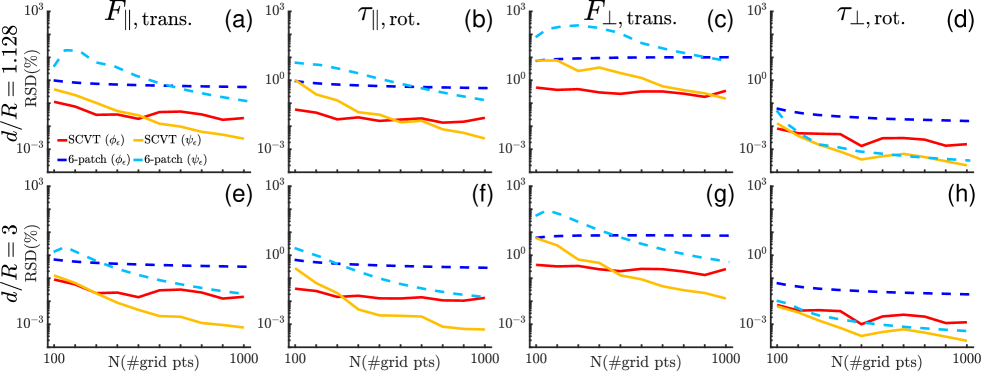
Figure 6: The figures show the relative standard deviation (RSD) (the standard deviation divided by the mean value) as a percentage versus number of discretization points, $N$, at $d/R=1.128$ (top row) and at $d/R=3$ (bottom row). Panels (a) and (e) are drag when moving parallel to the boundary, (b) and (f) are torque with the rotation axis parallel to the boundary, (c) and (g) are drag when moving perpendicular to the boundary, and (d) and (h) are torque with the rotation axis perpendicular to the boundary. The red and dark blue curves are simulations that used the $\phi_{\epsilon}$ regularization function, whereas the gold and cyan curves used the new $\psi_{\epsilon}$ regularization function. Each sphere motion was simulated 36 times with the sphere’s discretization rotated along a random axis and a random angle. Away from the boundary, all simulation types show a low percent error relative to the theory, see Fig. 5. However, the SCVT simulations show a lower RSD when compared with the six-patch simulations for most motion types, and the SCVT simulations that use the $\psi_{\epsilon}$ regularization function generally show the lowest RSD as $N$ becomes large. The RSD is largest for sphere motion perpendicular to the plane for all simulation types, and lowest for torque with the rotation axis perpendicular to the boundary for all simulation types, see also Figs. 7 and 8.

Comparison of the optimized simulations with experiment and theory

We used the high-order regularization function $\psi_{\epsilon}$, the SCVT discretization method ($N=1000$), and the free-space-optimized value for the regularization parameter to simulate sphere motion for a large range of boundary distances for comparison with the experiments and theory, as shown in Fig. 7 and Fig. 8.

The perpendicular translation, $F_{\perp}$, data in Fig. 7(a) shows that the data all agree for most boundary distances, except very near the boundary, which is consistent with what we found in the above analysis, see the top row of Fig. 5. In this region, the dimensionless drag increases by a factor nearly $10^{4}$. The distance moved between frames in the experiment is around $10\mu$m, which highlights the precision needed in the motion tracking. However, the inset shows that the numerical simulations diverge systematically from the theory and experiments when the sphere is very near the boundary, $d/R\approx 1.1$. We find the same systematic divergence from theory when using either $\phi_{\epsilon}$ or $\psi_{\epsilon}$ with the GSIRS, and find a similar result for the other three fundamental sphere motions, as described below.

Figure 7(b) shows that the parallel translation, $F_{\parallel}$, simulations perform better overall than the simulations of perpendicular translation. However, the inset shows a similar deviation from theory in the simulations at the about the same boundary distance $d/R=1.1$, which becomes much more pronounced by $d/R=1.05$. The maximum drag increase expected for this motion is a factor of about ten compared to about $10^{4}$ in the perpendicular translation case, which may explain why the deviation is less pronounced until the sphere is closer to the boundary.

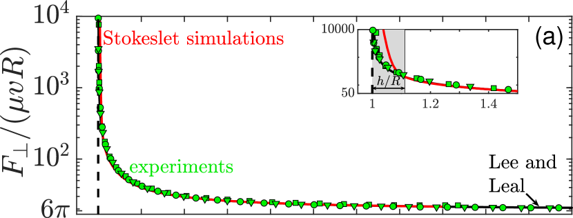
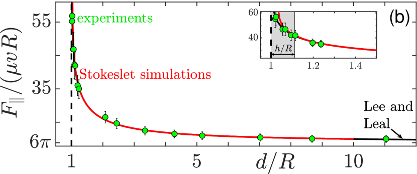
Figure 7: Dimensionless drag versus scaled boundary distance, $d/R$, on a sphere moving: (a) perpendicular to a boundary, $F_{\perp}/(\mu vR)$ and (b) parallel to a boundary $F_{\parallel}/(\mu vR)$, where $\mu$ is the dynamic viscosity, $v$ is the speed, $R$ is the radius of the sphere, and $d$ is the distance from the center of the sphere to the boundary. The solid black curve shows the theory by Lee and Leal [14], the solid red curve are optimized GSIRS simulations, and the solid green symbols are three dynamically similar experimental trials, which show the typical scatter in the data. The numerical simulations were optimized by using the optimal regularization parameter $\epsilon_{\rm free}$ from the combination of SCVT and $\psi_{\epsilon}$ that minimizes the percent error between theory and simulation in free space. The insets in both panel (a) and panel (b) show the data in the near boundary region where the simulation data diverge from the Lee and Leal theory, which occurs around $d/R=1.1$. The shaded boxes in the insets show $d/R=1.1=h/R+1$ where $h/R=0.11$ is the normalized average discretization size in the simulations. The simulations diverge from the theory and experiments around this distance for three of the four fundamental motions, see also Fig. 8.

Figure 8(a) shows that the three data types: theory, experiments, and simulations all agree very well for torque with the rotation axis perpendicular to the boundary, $\tau_{\perp}$. The deviation of the simulations from experiments and theory occurs much closer to the boundary and is smaller. Here we note that the motion of the regularized Stokeslets is strictly parallel to the boundary as the sphere rotates and that the translation data described above also showed better results when the motion was parallel to the boundary.

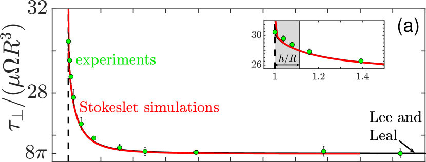
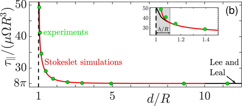
Figure 8: Dimensionless torque versus boundary distance $d$ scaled by the spherical radius $R$ for rotation with the axis: (a) perpendicular to the surface $\tau_{\perp}$ and (b) with the rotation axis parallel to the boundary $\tau_{\parallel}$. The theory by Lee and Leal are solid black curves, optimized GSIRS simulations are solid red curves, and dynamically similar experimental trials are solid green symbols. The experiments and simulations agree well with the theory when the boundary distance is greater than $d/R>1+h/R$, where $h$ is the average discretization size ($\approx$ distance between discretization points). The inset in panel (a) shows that the simulations perform better for perpendicular torque $\tau_{\perp}$. However, the panel (b) inset shows divergence of the simulations from theory, which is similar to the divergence shown in Fig. 7. The inset in panel (b) also shows that the experiments diverge from the theory in the near boundary region, but the divergence is likely due to difficulty in locating the edge of the sphere in the experiments, see Experimental Methods.

Torque with the rotation axis parallel to the boundary, $\tau_{\parallel}$, is shown in Fig. 8(b). The experiments show some systematic deviation from theory, which we attribute to uncertainty in locating the edge of the sphere to establish when $d/R=0$. The distance to the boundary for the closest experimental data point is $d/R=0.039$, which is $d=$0.5 mm in dimensional units. This distance is of the same order as the precession of the sphere under rotation, which is likely the cause. The simulations also show systematic deviation from theory at about $d/R=1.1$ in these data, as found in the other motions.

In summary, none of the simulation types perform well when the sphere is located very near the boundary, see the insets in Fig. 7 and Fig. 8. Other researchers such as Zheng et al. (2023) [33] have suggested that the method of images does not perform well when the size of the gap between the edge of an object and wall is smaller than the size of the regularization parameter $\epsilon$. In our data, the normalized gap size ($h/R=d/R-1=0.11$) where the numerical simulations diverge from the theory is larger than the optimal value of $\epsilon/R=0.042$ for $\phi_{\epsilon}$ and smaller than the optimal value of $\epsilon/R=0.27$ for $\psi_{\epsilon}$. Thus, the poor performance does not seem to be because the gap size from the edge of the sphere to the wall is within the size of the regularization parameter. Instead, we find that the GSIRS simulations for $N=1000$ in Fig. 7 and Fig. 8 diverge from theory when the gap size is within the average discretization size, $h/R=0.11$, or when the distance to the center of the sphere is $d/R<1.11$.

Minimizing error very near the boundary

Our approach to optimizing the simulations far from the boundary by using MRS calculations, as described in Numerical Methods, results in small percent errors for all boundary distances except when the sphere’s edge is closer to the boundary than a discretization length (insets of Fig. 7 and Fig. 8). We investigated this limitation of our optimization method by varying $N\in\{1000:200:2400\}$, and placing the sphere at $d=h+R$ to the wall. We simulated all four motions near the boundary using the $\psi_{\epsilon}$ regularization function for a range of $\epsilon$ values to find the the optimal regularization parameter at this distance, as shown in in Fig. 9. The near-boundary optimal regularization parameter at the distance $d=h+R$ is the one that minimizes the percent error between the simulations and the theory.

The presence of the boundary breaks the symmetry of motion in free space and results in four different optimal regularization parameters rather than two very similar values of $\epsilon_{\rm free}$, as found for translation and rotation, see Fig. 4(c)-(d). In free space, the values of $\epsilon_{\rm free}$ for translation (0.270) and rotation (0.248) differ by about 9% for $\psi_{\epsilon}$ with $N=1000$, whereas near the boundary the optimal values of $\epsilon$ vary by more than 50% for the different motions. Figure 9 also shows that the varying $N$ changes the size of the optimal regularization parameter because the minima occur at different locations $h$. Thus, not only does the average discretization size $h$ provide the threshold for the minimum gap between the edge of the sphere and the wall, but also the optimal regularization parameter depends on $h$ near the boundary.

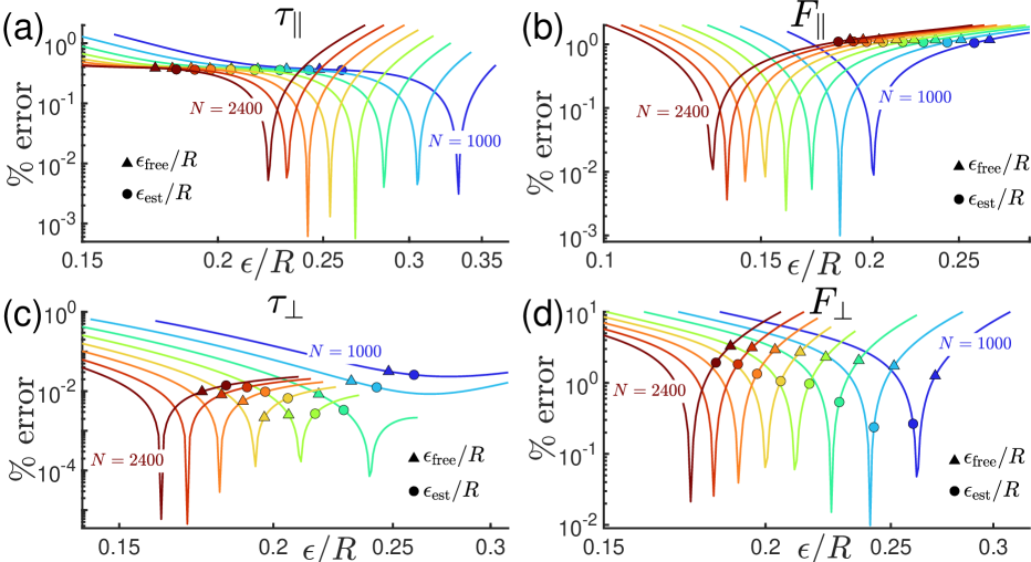
Figure 9: Optimizing the regularization parameter $\epsilon$ when the edge of the sphere is one discretization length $h$ from the boundary. The simulations use the SCVT discretization method and the $\psi_{\epsilon}$ regularization function for eight values of $N$ from 1000 to 2400 in increments of 200 corresponding to eight different discretization lengths $h$. The solid curves are the percent error as the regularization parameter is varied for each value of $N$, which all show a clear minimum that could be used to minimize the difference between simulations and theory, see Fig. 10. By contrast, solid triangles are the free-space-optimized values of $\epsilon_{\rm free}/R$ found using the MRS simulations, as described in Optimal regularization parameter section, above. The solid circles are the estimated values of $\displaystyle\epsilon_{\rm est}/R=3/2(h/R)^{4/5}$ using the fit function as described in Fig. 4. Using either the free-space-optimized or the estimated value of the regularization parameter introduces a small percent difference relative to theory near the boundary, but slightly better performance further from the boundary.

Assuming $h$ is small, i.e., the sphere is moving near the boundary, we can Taylor expand the regularization parameter for each fundamental motion to first order,

$$\epsilon(h)\approx\epsilon(0)+\left.\frac{d\epsilon}{dh}\right|_{h=0}h$$ (8)

In Fig. 10, we show the results of optimizing $\epsilon$ at a boundary distance equal to the discretization length $h$ over a range of values and fitting Eq. 8 to the data. Near the boundary, small changes in $\epsilon$ lead to large changes in the percent error, while far from the boundary, the percent error is less sensitive to changes in $\epsilon$ (Fig. 3). Note that the log scale in the vertical makes the rate of change in percent error as $\epsilon$ varies appear to be very rapid, but the slope of the curves in Fig. 3 near the minimum is typically 10, whereas in Fig. 9 the slopes are of order $10^{-7}$ or smaller. Therefore, when a particular simulation requires some motion to be near a boundary, an alternative approach to reduce error is to determine the closest distance desired a priori and then to optimize the regularization parameter at that distance; motion further from the surface using same regularization parameter value will also have small errors. For the motion of a sphere, the fit values shown in Fig. 10 may be used to determine appropriate regularization parameters, though each component of motion would have to be simulated separately with a different value of $\epsilon$. This requirement makes our free-space optimization method a better choice in most situations.

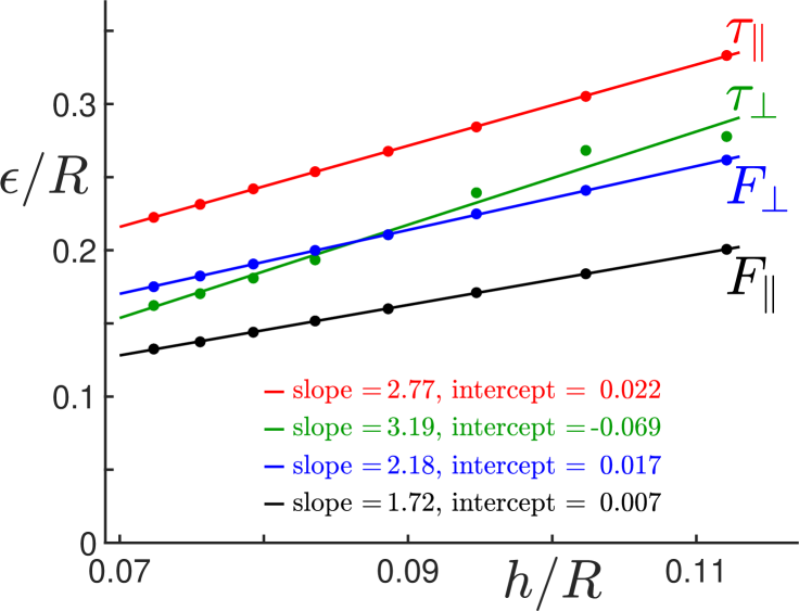
Figure 10: Optimal regularization parameter $\epsilon$ plotted as a function of discretization length $h$. In these data, the edge of the sphere is located at a distance $h$ from the boundary. Optimal regularization parameters are found for each of the four motion types by identifying the minima of the curves shown in Fig. 9. The solid curves are linear fits to the data with coefficients shown. The data are fit very well except in the case of perpendicular translation $F_{\perp}$, which shows some scatter from the linear fit for the three lowest resolutions: $N=$ 1000, 1200, and 1400. The data show that there is no single optimal choice for the regularization parameter once the sphere is near the boundary. Whereas in free space, the optimal value of the regularization parameter is more similar for translation and rotation, as shown in Fig. 4.

Discussion

The goal of this work is to provide researchers with a method to precisely calibrate the method of images for regularized Stokeslets simulations of spheres moving near a boundary using measurements of forces and torques from macroscopic experiments and values from the bipolar coordinate theory by Lee and Leal [14]. We chose this theory because of its comprehensive nature though other analyses give the same predictions, see for example [11, 12, 13]. We expect bipolar coordinate theories to be accurate because they are exact solutions to the Navier Stokes equations, but they assume a Reynolds number of zero and that the sphere is moving near an infinite plane, so their utility in an experiment was largely untested prior to this work. Our results provide the first comprehensive experimental test of these theories, and Figures 7 and 8 show that the theory can be used to effectively remove the finite size effects in an experiment, at least for the size of our tank, which is approximately $48R\times 48R\times 30R$. Considering the significant contribution ($\gtrsim 10\%$) to the predicted drag and that the tank has corners, etc., the theory worked very well despite its underlying assumptions.

Using the verified theory, we developed computational methods to accurately represent a sphere moving near a boundary, as a model of a spherical swimmer or a sedimenting particle. Our method of finding the optimal regularization parameter, $\epsilon_{\rm free}$, provides a computationally efficient way to optimize the method of images for regularized Stokeslets, whether using the $\phi_{\epsilon}$ or the $\psi_{\epsilon}$ regularization function, though we find the latter to be a better choice because of its stability, convergence, and error properties, as shown in Fig. 5. We found fit functions that allow researchers to bypass the optimization process, and instead, use Eq. (6) to set a value of $\epsilon$ when using $\phi_{\epsilon}$ and Eq. (7) when using $\psi_{\epsilon}$. The relationship between average discretization size and regularization parameter we found for spheres when compared to the results for cylinders found by Shindell et al. (2023) [3] confirms their result that the relationship between discretization size and regularization parameter depends on the shape of the simulated object.

We also show that the SCVT discretization method is superior to the six-patch method: it generally provides more accurate results because it distributes points more uniformly on the surface of the sphere, see Fig. 3 and Fig. 5. The nonuniformity of the six-patch point distribution also causes significantly increased variance in the computed values when the sphere is rotated with respect to the boundary, as shown in Fig. 6. Thus, a discretization method that creates a nearly uniform point distribution should be chosen for simulations of a sphere moving near a boundary.

In our work, the method of images lost accuracy when the sphere was located near the boundary, see the insets in Fig. 7 and Fig. 8. Zheng et al. (2023) [33] commented that the image system may suffer inaccuracy within a distance of order of the regularization parameter due to the non-zero values of the image sources crossing the boundary. While the force distribution is modified near the wall due to the presence of the image system, we find that the relevant length scale is the gap size relative to the average discretization length, $h$, rather than the gap size relative to the size of the regularization parameter, $\epsilon$. Our GSIRS simulations using the same $\phi_{\epsilon}$ regularization function as Zheng et al. used, show high percent errors from theory when the distance of the edge of the sphere was larger than the size of the regularization parameter, see the top row of Fig. 5. At this location, the gap is much larger than the optimized regularization parameter; the gap is 0.089R and the regularization parameter is $\epsilon=0.042R$. Furthermore, we found that when using $\psi_{\epsilon}$ at the same distance there are large differences relative to theory, and in this case, the gap is much smaller than the size of the regularization parameter: $\epsilon=0.27R$. Our finding was that the simulations lost accuracy when the gap between the edge of the sphere and the boundary was smaller than the discretization size $h$.

This inaccuracy in the simulations near the boundary led us to find an empirical rule for establishing the number of grid points necessary when discretizing a sphere: determine the closest distance to the boundary that will be simulated and ensure that the average discretization length is smaller than this distance. Our method of optimizing the simulations in free space and this discretization rule will give better results than using the size of the regularization parameter to establish the limits of accuracy. It is unknown whether this empirical discretization rule is relevant for other geometries, but will be the subject of future tests.

We also optimized the regularization parameter with the sphere located at $d/R=1+h/R$ by minimizing the percent error relative to theory at this near-boundary location. Figure 10 shows that there is a linear relationship between $\epsilon$ and $h$, but the optimal regularization parameter depends strongly on motion type. Simulating arbitrary motion near a boundary using this method would require dynamically changing the regularization parameter value depending on how the sphere is moving. Alternately, the motion could be decomposed into components of translation and rotation, each component of motion simulated independently, and the results summed to give the final result. However, decomposing the motion into components would have limited value because the components could be calculated directly from theory for a given boundary distance, rotation, and velocity. Thus, in most situations we consider the free-space-optimization a better choice because of its simplicity and computational efficiency.

In conclusion, using the GSIRS with a uniform point distribution such as the SCVT, a high-order regularization parameter function such as $\psi_{\epsilon}$, and a free-space-optimized regularization parameter provides an efficient and generally very accurate method for simulating spheres moving near a boundary providing the edge of the sphere is kept outside of the average discretization length. This result along with our experimental validation of theory and MATLAB and PYTHON implementations of the Lee and Leal theory provide important resources for other researchers using the GSIRS or other simulation methods to assess the accuracy of their numerical results. Future study should explore how our optimization strategy and calibration process work for other geometries including compound objects such as a sphere with a helical flagellum.

Author Information

Authors and Affiliations

Physics Program, Centre College of Kentucky, Danville, KY 40422, USA

Kathleen Brown, Jonathan McCoy, and Bruce Rodenborn

Department of Mathematics, Tulane University, New Orleans, LA 70118, USA

Ricardo Cortez

Department of Mathematics, Trinity University, San Antonio, TX, 78212, USA

Hoa Nguyen and Amelia Gibbs

Department of Physics and Astronomy, Trinity University, San Antonio, TX, 78212, USA

Orrin Shindell

Department of Biology, Trinity University, San Antonio, TX, 78212, USA

Frank Healy

Contributions

B.R., H.N., R.C., O.S., and F.H. were involved in conceptualization of the project. For the original draft, B.R. wrote, reviewed, and edited the manuscript while H.N. and R.C. wrote the Numerical Methods section. B.R., H.N., R.C., and O.S. worked together on revising the final draft. B.R. designed the experiments and analyzed the results. B.R. and O.S. created the numerical implementation of theory in MATLAB. B.R. mentored two undergraduate students (K.B. and J.M) to conduct experiments, analyze the results, and assist in developing the supplementary information including a PYTHON version of the theory. H.N. designed the numerical codes, and mentored one undergraduate student (A.G.) on model development and implementation to generate simulation results and data analysis. A.G. conducted simulations and analyzed the results. R.C. provided the regularization function $\psi_{\epsilon}$ and insights into the GSIRS. All authors reviewed the manuscript.

Additional information

Competing interests

The authors declare no competing interests.

Data Availability

The data presented in this manuscript are provided via GOOGLE DRIVE at https://drive.google.com/drive/folders/1w-U42eVbh17HiOrBwUJB6SW0ttMy6n0s?usp=share_link. Other data and numerical simulation code that support the findings of this study are available from the corresponding author upon reasonable request.

Numerical implementation of Lee and Leal theory

The bipolar coordinate theory by Lee and Leal (1980) [14] gives a series solution to the force and torque on a sphere moving near an infinite boundary and includes a slip coefficient $\lambda$ that represents the degree of slip at the boundary from no-slip $\lambda=\infty$ to free-slip $\lambda=0$. We solve their equations listed below using both MATLAB and PYTHON GUI programs for convenience. The MATLAB code includes a GUI interface using MATLAB’s AppDesigner functionality tested on R2021 and later. We also provide a PYTHON GUI program that contains the same basic features tested on PYTHON 3.12.1, which requires the PySimpleGUI, numpy, and pyperclip packages. The inputs to the GUI’s are:

1. Radius of the sphere: the default is unity since all values are scaled using the radius.

2. Viscosity ratio: the range is $0>\lambda\leq\infty$. The default is "inf", i.e. infinity, which is equivalent to a no slip boundary near the sphere. Implementing $\lambda=0$ was only included for perpendicular torque calculations since Lee and Leal developed an analytic expression. Otherwise, a very small nonzero value should be used in this limit.

3. Number of terms: this is the truncation value for the infinite sums.

4. Boundary distances: range $1<l=d/R\leq\infty$. These are boundary distances at which the theoretical values will be calculated. Dimensional values will be scaled by the sphere radius. When $l/R=1$, the theory diverges.

5. Motion type: there are four radio buttons provided for selecting which of the four fundamental types of motion are to be calculated

The MATLAB GUI calls one of three primary functions, for which we have also coded PYTHON equivalents:

1. motion_parallel.m and motion_parallel.py: calculate the force and torque for rotation or translation parallel to a plane interface.The inputs are: $l$, $\lambda$, $N$ and motion, where motion=2 is for translation and motion=4 is for rotation following the notation in Lee and Leal.

2. rotation_perpendicular.m and rotation_perpendicular.py: calculate the torque for rotation perpendicular to the boundary. The inputs are: $l$, $\lambda$, and $N$. Here all force components are zero.

3. translation_perpendicular.m and translation_perpendicular.py: calculate the additional drag force for motion perpendicular to a plane interface. The inputs are: $l$, $\lambda$, and $N$. Here all torques are zero.

The outputs from the function are the increase in the vector force and torque components so conversion to dimensional units is done by multiplying all force values by the Stokes drag $6\pi\mu Rv$ and by multiplying all torque values by the torque on a sphere far from a boundary $8\pi\mu R^{3}\Omega$, where $\mu$ is the viscosity of the fluid, $R$ the radius of the sphere, $v$ is the speed of the sphere, and $\Omega$ is the angular frequency.

Below are the system of equations developed by Lee and Leal that are solved in our MATLAB and PYTHON codes [14]. We have preserved their numbering for easy reference and included comments in the MATLAB and PYTHON codes that identify how each equation is used.

In their work, translation perpendicular to a plane interface or rotation with axis perpendicular to the interface, result in $m=0$, whereas parallel motion results in $m=1$, in the equations below.

The equations result in seven unknown coefficients: $A_{n}^{m}$, $B_{n}^{m}$, $C_{n}^{m}$, $E_{n}^{m}$, $F_{n}^{m}$, $G_{n}^{m}$, and $H_{n}^{m}$. They note that $D_{n}^{m}=\hat{D}_{n}^{m}=\hat{C}_{n}^{m}=0$ because of equations (32) and (37) below. There are seven unknown coefficients for the other fluid denoted as $\hat{A}^{m}_{n}$, $\hat{B}^{m}_{n}$, $\hat{C}^{m}_{n}$, $\hat{D}^{m}_{n}$, $\hat{E}^{m}_{n}$, $\hat{F}^{m}_{n}$, $\hat{G}^{m}_{n}$, and $\hat{H}^{m}_{n}$.

$$l\equiv d/R\qquad\qquad(2)$$

$$\eta_{0}=-\cosh^{-1}(l)\qquad\text{see pg. 205}$$

for the upper fluid and all $n$ and $m$:

$$\hat{A}^{m}_{n}=-\hat{B}^{m}_{n},\ \hat{C}^{m}_{n}=-\hat{D}^{m}_{n},\ \hat{E}^{m}_{n}=-\hat{F}^{m}_{n},\ \text{ and }\ \hat{G}^{m}_{n}=-\hat{H}^{m}_{n}$$ (32)

for $m=0$

$$-\frac{1}{2}nA^{0}_{n-1}+\frac{5}{2}A^{0}_{n}+\frac{1}{2}(n+1)A^{0}_{n+1}-nD^{0}_{n-1}+(2n+1)D^{0}_{n}-(n+1)D^{0}_{n+1}$$

$$+n(n-1)E^{0}_{n-1}-2n(n+1)E^{0}_{n}+(n+1)(n+2)E^{0}_{n+1}=0$$

and

$$-\frac{1}{2}nB^{0}_{n-1}+\frac{5}{2}B^{0}_{n}+\frac{1}{2}(n+1)B^{0}_{n+1}-nC^{0}_{n-1}+(2n+1)C^{0}_{n}-(n+1)C^{0}_{n+1}$$

$$+n(n-1)F^{0}_{n-1}-2n(n+1)F^{0}_{n}+(n+1)(n+2)F^{0}_{n+1}=0$$

while for $m\geqslant 1,$:

$$-\frac{1}{2}(n-m)A^{m}_{n-1}+\frac{5}{2}A^{m}_{n}+1/2(n+m+1)A^{m}_{n+1}-(n-m)D^{m}_{n-1}+(2n+1)D^{m}_{n}$$

$$-(n+m+1)D^{m}_{n+1}+\frac{1}{2}(n-m)(n-m-1)E^{m}_{n-1}-(n-m)(n+m+1)E^{m}_{n}$$

$$+\frac{1}{2}(n+m+1)(n+m+2)E^{m}_{n+1}-\frac{1}{2}G^{m}_{n-1}+G^{m}_{n}-\frac{1}{2}G^{m}_{n+1}=0$$

and

$$-\frac{1}{2}(n-m)B^{m}_{n-1}+\frac{5}{2}B^{m}_{n}+1/2(n+m+1)B^{m}_{n+1}-(n-m)C^{m}_{n-1}+(2n+1)C^{m}_{n}$$

$$-(n+m+1)C^{m}_{n+1}+\frac{1}{2}(n-m)(n-m-1)F^{m}_{n-1}-(n-m)(n+m+1)F^{m}_{n}$$

$$+\frac{1}{2}(n+m+1)(n+m+2)F^{m}_{n+1}-\frac{1}{2}H^{m}_{n-1}+H^{m}_{n}-\frac{1}{2}H^{m}_{n+1}=0$$

$$D^{m}_{n}=\hat{D}^{m}_{n}=0\qquad\text{for all}\quad n,m.$$ (37)

for all $m$, $\eta$ and $\xi$, we require:

$$-\frac{(n-m-1)}{2n-1}(F^{m}_{n-1}-\hat{F}^{m}_{n-1})+(F^{m}_{n}-\hat{F}^{m}_{n})-\frac{n+m+2}{2n+3}(F^{m}_{n+1}-\hat{F}^{m}_{n+1})$$

$$=\frac{1}{2}\left[\frac{1}{2n-1}(B^{m}_{n-1}-\hat{B}^{m}_{n-1})-\frac{1}{2n+3}(B^{m}_{n+1}-\hat{B}^{m}_{n+1}\right]$$

$$\text{for }m=0:\quad H^{0}_{n}=\hat{H}^{0}_{n}$$ (41a)

for $m\geqslant 1$:

$$-\frac{(n-m-1)}{2n-1}(H^{m}_{n-1}-\hat{H}^{m}_{n})+(H^{m}_{n}-\hat{H}^{m}_{n})-\frac{n+m}{2n+3}(H^{m}_{n+1}-\hat{H}^{m}_{n+1})$$

$$=-\frac{1}{2}\left[-\frac{(n-m)(n-m+1)}{2n-1}(B^{m}_{n-1}-\hat{B}^{m}_{n-1})-\frac{(n+m)(n+m+1)}{2n+3}(B^{m}_{n+1}-\hat{B}^{m}_{n+1})\right]$$

for $m=0$:

$$G^{0}_{n}=\lambda\hat{G}^{0}_{n}$$ (45a)

for all $m$:

$$E^{m}_{n}\sinh{(n+1/2)}\eta_{0}+F^{m}_{n}\cosh{(n+1/2)}\eta_{0}=X^{m}_{n}(\eta_{0})-\frac{1}{(2n+3)\sinh{\eta_{0}}}[-Z^{m}_{n+1}(\eta_{0})$$

$$+C^{m}_{n+1}\sinh{(n+3/2)}\eta_{0}]+\frac{1}{(2n-1)\sinh{\eta_{0}}}[-Z^{m}_{n-1}(\eta_{0})]$$

$$+C^{m}_{n-1}\sinh{(n-1/2)}\eta_{0}]$$

for $m=0$:

$$G^{0}_{n}\sinh{(n+1/2)}\eta_{0}+H^{0}_{n}\cosh{(n+1/2)}\eta_{0}=Y^{0}_{n}(\eta_{0})$$ (55a)

for $m\geqslant 1$:

$$G^{m}_{n}\sinh{(n+1/2)}\eta_{0}+H^{m}_{n}\cosh{(n+1/2)}\eta_{0}$$

$$=Y^{m}_{n}(\eta_{0})+\frac{(n+m)(n+m+1)}{(2n+3)\sinh{\eta_{0}}}[-Z^{m}_{n+1}(\eta_{0})+C^{m}_{n+1}\sinh{(n+3/2)}\eta_{0}]$$

$$-\frac{(n-m)(n-m+1)}{(2n-1)\sinh{\eta_{0}}}[-Z^{m}_{n-1}(\eta_{0})+C^{m}_{n-1}\sinh{(n-1/2)}\eta_{0}]$$ (55b)

for all $m$:

$$A^{m}_{n}\sinh{(n+1/2)}\eta_{0}+B^{m}_{n}\cosh{(n+1/2)}\eta_{0}=\frac{-2}{\sinh{\eta_{0}}}[\frac{(n-m)}{2n-1}\{Z^{m}_{n-1}(\eta_{0})$$

$$-C^{m}_{n-1}\sinh{(n-1/2)}\eta_{0}\}-\cosh{\eta_{0}}\{Z^{m}_{n}(\eta_{0})-C^{m}_{n}\sinh{(n+1/2)\eta_{0}}\}$$

$$+\frac{n+m+1}{2n+3}\{Z^{m}_{n+1}(\eta_{0})-C^{m}_{n+1}\sinh{(n+3/2)\eta_{0}}\}]$$

and

$$A^{m}_{n}=\lambda\hat{A}^{m}_{n},\quad E^{m}_{n}=\lambda\hat{E}^{m}_{n}\quad and\quad G^{m}_{n}=\lambda\hat{G}^{m}_{n}.$$ (57)

The equations are rewritten so that the LHS has only coefficients, and all other terms are on the RHS. The matrix is constructed using a for-loop, where each column is built as shown in Eq. 58. The first column ($n=m-1$) and last column ($n=N+1$) are removed after construction because the sums should range from $\sum_{n=m}^{N}$, where $N$ is a truncation value chosen for a desired accuracy. The result is a square, banded matrix of size $N\times N$. The rows and columns are constructed in columns as:

$$\begin{pmatrix}\par n-1&n&n+1&\dots&N+2\\ A^{m}_{(n-1)}&\dots\\ &A^{m}_{n}&\dots\\ &&A^{m}_{(n+1)}&\dots\\ B^{m}_{(n-1)}&\dots\\ &B^{m}_{n}&\dots\\ &&B^{m}_{(n+1)}&\dots\\ \vdots\end{pmatrix}$$ (58)

The resulting matrix is inverted and multiplied times the RHS to solve for the coefficients. The force and/or torque for the four fundamental motions are calculated using the following equations:

1. Force for perpendicular translation:

   $$F_{x}=F_{y}=0,$$

   $$F_{z}=\frac{-\sqrt{2}}{3}\sinh{\eta_{0}}\sum_{n}[C_{n}^{0}-(n+1/2)(A_{n}^{0}-B_{n}^{0})]$$

   $$\tau_{x}=\tau_{y}=\tau_{z}=0,$$

2. Force and torque for parallel translation:

   $$F_{y}=F_{z}=0,$$

   $$F_{x}=\frac{-\sqrt{2}}{6}\sinh{\eta_{0}}\sum_{n}[G_{n}^{1}-H_{n}^{1}+n(n+1)(A_{n}^{1}-B_{n}^{1})]$$

   $$\tau_{x}=\tau_{z}=0,$$

   $$\tau_{y}=\frac{\sinh^{2}{\eta_{o}}}{12\sqrt{2}}\sum_{n}[2+e^{(2n+1)\eta_{0}}\{n(n+1)(-2C_{n}^{1}-A_{n}^{1}\coth{\eta_{0}})$$

   $$-(2n+1+\coth{\eta_{0}})G_{n}^{1}\}+(2-e^{(2n+1)\eta_{0}})\{n(n+1)B_{n}^{1}\coth{\eta_{0})}$$

   $$+(2n+1+\coth{\eta_{0}})H_{n}^{1}\}].$$

3. Torque for perpendicular axis rotation

   $$F_{x}=F_{y}=F_{z}=0$$ (82)

   $$\tau_{x}=\tau_{y}=0,$$

   $$\tau_{z}=\frac{\sinh^{2}{\eta_{0}}}{\sqrt{2}}\sum_{n}n(n+1)(-G_{n}^{0}+H_{n}^{0}).$$ (83)

4. Force and torque for parallel axis rotation

   $$F_{x}=\frac{-\sqrt{2}}{6}\sinh{\eta_{0}}\sum_{n}[G_{n}^{1}-H_{n}^{1}+n(n+1)(A_{n}^{1}-B_{n}^{1})],$$

   $$F_{y}=F_{z}=0$$

   $$\tau_{x}=\tau_{z}=0,$$

   $$\tau_{y}=-\frac{1}{3}-\frac{\sinh^{2}{\eta_{0}}}{12\sqrt{2}}\sum_{n}[(2+e^{2n+1)\eta_{0}})$$

   $$\times\{n(n+1)(-2C_{n}^{1}-A_{n}^{1}\coth{\eta_{0}})$$

   $$-(2n+1+\coth{\eta_{0}})G_{n}^{1}\}$$

   $$+(2-e^{(2n+1)\eta_{0}}\{n(n+1)B_{n}^{1}\coth{\eta_{0}}+(2n+1+\coth{\eta_{0}}H_{n}^{1}\}].$$ (87)

The MATLAB and PYTHON codes can solve the series solutions quickly even when $10^{4}$ terms are included using a computer with 16GB of RAM. This number of terms is only necessary for very small boundary distances and changes the result in 5-6 digit, whereas for many cases $N=100$ is sufficient.

We compared our results from Lee and Leal[14] with the values from our calculations using $N=500$ terms and found that the maximal difference is in the sixth digit of accuracy and is generally in the seventh or eigth digit. Our code does not implement $\lambda=0$, so the values used $\lambda=10^{-8}$. At this level of precision, it is unclear whose calculations are correct, but the results show that the numerical implementation matches the work of Lee and Leal to a high degree of accuracy. We note that they appear to have a mistake in the value for $\lambda=10$ and $l=1.6$, which we believe should be $\tau=-5.26852\times 10^{-5}$, but is reported as being $\tau=-5.26852\times 10^{-3}$. The former value matches our results very well, as do all of the other values in the table, so we believe the value in the table is incorrect. The supplementary materials include a MATLAB script (Lee_and_Leal_tabulated_values.m) that calculates these differences, which are available here:

https://drive.google.com/drive/folders/1w-U42eVbh17HiOrBwUJB6SW0ttMy6n0s?usp=share_link.

References

- Cortez and Varela [2015] R. Cortez and D. Varela, A general system of images for regularized stokeslets and other elements near a plane wall, Journal of Computational Physics 285, 41 (2015).
- Cortez et al. [2005] R. Cortez, L. Fauci, and A. Medovikov, The method of regularized Stokeslets in three dimensions: Analysis, validation, and application to helical swimming, Phys. Fluids 17, 0315041 (2005).
- Shindell et al. [2021] O. Shindell, H. Nguyen, N. Coltharp, F. Healy, and B. Rodenborn, Using experimentally calibrated regularized Stokeslets to assess bacterial flagellar motility near a surface, Fluids 6 (2021).
- Purcell [1997] E. M. Purcell, The efficiency of propulsion by a rotating flagellum, Proc. Natl. Acad. Sci. 94, 11307 (1997).
- Li and Tang [2006] G. Li and J. X. Tang, Low flagellar motor torque and high swimming efficiency of caulobacter crescentus swarmer cells, Biophys. J. 91, 2726 (2006).
- Li et al. [2017] C. Li, B. Qin, A. Gopinath, P. E. Arratia, B. Thomases, and R. D. Guy, Flagellar swimming in viscoelastic fluids: role of fluid elastic stress revealed by simulations based on experimental data, J. R. Soc. Interface 14, 20170289 (2017).
- Manson et al. [1980] M. D. Manson, P. M. Tedesco, and H. C. Berg, Energetics of flagellar rotation in bacteria, Journal of Molecular Biology 138, 541 (1980).
- Imhoff et al. [1984] J. F. Imhoff, H. G. Truper, and N. Pfennig, Rearrangement of the species and genera of the phototrophic “purple nonsulfur bacteria”, International Journal of Systematic and Evolutionary Microbiology 34, 340 (1984).
- Turner et al. [2016] L. Turner, L. Ping, M. Neubauer, and H. C. Berg, Visualizing flagella while tracking bacteria, Biophysical Journal 111, 630 (2016).
- Jeffery [1915] G. B. Jeffery, On the steady rotation of a solid of revolution in a viscous fluid, Proc. London Math. Soc. s2_14, 327 (1915).
- Brenner [1961] H. Brenner, The slow motion of a sphere through a viscous fluid towards a plane surface, Chem. Eng. Sci. 16, 242 (1961).
- O’Neill [1964] M. E. O’Neill, A slow motion of viscous liquid caused by a slowly moving solid sphere, Mathematika 11, 67 (1964).
- Dean and O’Neill [1963] W. R. Dean and M. E. O’Neill, A slow motion of viscous liquid caused by the rotation of a solid sphere, Mathematika 10, 13 (1963).
- Lee and Leal [1980] S. H. Lee and L. G. Leal, Motion of a sphere in the presence of a plane interface. part 2. an exact solution in bipolar co-ordinates, J. Fluid Mech. 98, 193 (1980).
- O’Neill and Bhatt [1991] M. E. O’Neill and B. S. Bhatt, Slow motion of a solid sphere in the presence of a naturally permeable surface, Q. J. Mech. Appl. Math. 44, 91 (1991), https://academic.oup.com/qjmam/article-pdf/44/1/91/5381263/44-1-91.pdf .
- Chaoui and Feuillebois [2003] M. Chaoui and F. Feuillebois, Creeping Flow around a Sphere in a Shear Flow Close to a Wall, Q. J. Mech. Appl. Math. 56, 381 (2003), https://academic.oup.com/qjmam/article-pdf/56/3/381/5226028/560381.pdf .
- Małysa and van de Ven [1986] K. Małysa and T. G. M. van de Ven, Rotational and translational motion of a sphere parallel to a wall, Int. J. Multiph. Flow 12, 459 (1986).
- Dufresne et al. [2000] E. R. Dufresne, T. M. Squires, M. P. Brenner, and D. G. Grier, Hydrodynamic coupling of two brownian spheres to a planar surface, Phys. Rev. Lett. 85, 3317 (2000).
- Pitois et al. [2009] O. Pitois, C. Fritz, L. Pasol, and M. Vignes-Adler, Sedimentation of a sphere in a fluid channel, Phys. Fluids 21, 103304 (2009), https://pubs.aip.org/aip/pof/article-pdf/doi/10.1063/1.3253408/13617731/103304_1_online.pdf .
- Wang et al. [2009] G. M. Wang, R. Prabhakar, and E. M. Sevick, Hydrodynamic mobility of an optically trapped colloidal particle near fluid-fluid interfaces, Phys. Rev. Lett. 103, 248303 (2009).
- Wu et al. [2021] H. Wu, F. Romano, and H. Kuhlmann, Attractors for the motion of a finite-size particle in a two-sided lid-driven cavity, J. Fluid Mech. 906, 10.1017/jfm.2020.768 (2021).
- Maxworthy [1965] T. Maxworthy, An experimental determination of the slow motion of a sphere in a rotating, viscous fluid, J. Fluid Mech. 23, 373 (1965).
- Kunesh et al. [1985] J. G. Kunesh, H. Brenner, M. E. O’Neill, and A. Falade, Torque measurements on a stationary axially positioned sphere partially and fully submerged beneath the free surface of a slowly rotating viscous fluid, J. Fluid Mech. 154, 29 (1985).
- Du et al. [2003] Q. Du, M. D. Gunzburger, and L. Ju, Constrained centroidal voronoi tessellations for surfaces, SIAM Journal on Scientific Computing 24, 1488 (2003), https://doi.org/10.1137/S1064827501391576 .
- Jeffrey and Onishi [1981] D. J. Jeffrey and Y. Onishi, The slow motion of a cylinder next to a plane wall., Q. J. Mech. Appl. Math. 34, 129 (1981).
- Nguyen and Cortez [2014] H.-N. Nguyen and R. Cortez, Reduction of the regularization error of the method of regularized stokeslets for a rigid object immersed in a three-dimensional stokes flow, Comput. Phys. Commun. 15, 126 (2014).
- Smith [2018] D. J. Smith, A nearest-neighbour discretisation of the regularized stokeslet boundary integral equation, J. Comput. Phys. 358, 88 (2018).
- Gallagher and Smith [2021] M. T. Gallagher and D. J. Smith, The art of coarse Stokes: Richardson extrapolation improves the accuracy and efficiency of the method of regularized stokeslets, R. Soc. Open Sci. 8, 210108 (2021), arXiv:2101.09286 [math.NA] .
- Beale [2001] J. Beale, A convergent boundary integral method for three-dimensional water waves, Mathematics of computation 70, 977 (2001).
- Ainley et al. [2008] J. Ainley, S. Durkin, R. Embid, P. Boindala, and R. Cortez, The method of images for regularized Stokeslets, Journal of Computational Physics 227, 4600 (2008).
- Smith [2009] D. J. Smith, A boundary element regularized stokeslet method applied to cilia-and flagella-driven flow, Proc. R. Soc. London, Ser. A 465, 3605 (2009).
- [32] Lili Ju’s website, https://people.math.sc.edu/ju/.
- Zheng et al. [2023] P. Zheng, D. Apsley, S. Zhong, J. Sznitman, and A. Smits, Image systems for regularised stokeslets at walls and free surfaces, Eur. J. Mech. B Fluids 97, 112 (2023).