A Unified Study on Sequentiality in Universal Classification with Empirically Observed Statistics

Abstract

In hypothesis testing problems, taking samples sequentially and stopping opportunistically to make the inference greatly enhances the reliability. The design of the stopping and inference policy, however, critically relies on the knowledge of the underlying distribution of each hypothesis. When the knowledge of distributions, say, $P_{0}$ and $P_{1}$ in the binary-hypothesis case, is replaced by empirically observed statistics from the respective distributions, the gain of sequentiality is less understood when subject to universality constraints. In this work, the gap is mended by a unified study on sequentiality in the universal binary classification problem. We propose a unified framework where the universality constraints are set on the expected stopping time as well as the type-I error exponent. The type-I error exponent is required to achieve a pre-set distribution-dependent constraint $\lambda(P_{0},P_{1})$ for all $P_{0},P_{1}$. The framework is employed to investigate a semi-sequential and a fully-sequential setup, so that fair comparison can be made with the fixed-length setup. The optimal type-II error exponents in different setups are characterized when the function $\lambda$ satisfies mild continuity conditions. The benefit of sequentiality is shown by comparing the semi-sequential, the fully-sequential, and the fixed-length cases in representative examples of $\lambda$. Conditions under which sequentiality eradicates the trade-off between error exponents are also derived.

I Introduction

It is known that sequentiality in taking samples greatly enhances reliability in statistical inference. Take the binary hypothesis testing problem as an example. The decision maker observes a sequence of samples drawn i.i.d. from one of the two known distributions $P_{0}$ or $P_{1}$. It aims to infer from which of the two distributions the sequence is generated. Both type-I and type-II error probabilities vanish exponentially fast as the number of samples $n$ tends to infinity, and the exponential rates are denoted as the error exponents, between which there exists a fundamental trade-off [1]. When samples are taken sequentially and the decision maker is free to decide when to stop as long as the expected stopping time is less than a given constraint $n$ [2, 3], the error exponents can simultaneously achieve the two extremes, namely, the two KL divergences $\mathrm{D}\mkern-1.5mu\left(P_{1}\middle\|P_{0}\right)$ and $\mathrm{D}\mkern-1.5mu\left(P_{0}\middle\|P_{1}\right)$. In words, sequentiality in taking samples eradicates the trade-off between error exponents. The optimal design of the stopping and inference strategies, however, critically relies on the knowledge of the underlying distributions [2, 3, 4].

In this work, we aim to investigate the benefit of sequentiality when the underlying distributions are unknown to the decision maker. Instead, the decision maker only has access to empirical statistics of training sequences sampled from these distributions, say, $P_{0}$ and $P_{1}$ in the binary-hypothesis case. Since the underlying distributions are unknown, it is natural to ask for a universal guarantee on certain performances. One such framework focused on the asymptotic performance as the number of samples in all sequences tend to infinity was proposed and studied by Ziv [5], where a universality constraint was set on the type-I error exponent to be no less than a given constant $\lambda_{0}>0$ regardless of the underlying distributions. Gutman [6] later proved the asymptotic optimality of Ziv’s universal test in the sense that it attains the optimal type-II error exponent (as a function of $P_{0},P_{1},\lambda_{0}$). Further extension was made by Levitan and Merhav [7] where a competitive criterion was taken, replacing the constant constraint $\lambda_{0}$ by a distribution-dependent one, $\lambda(P_{0},P_{1})$. From these results in the fixed-length settings, it can be seen that there still exists a trade-off between the two error exponents. A natural question emerges: in this universal classification problem, can sequentiality improve the trade-off, and even eradicate them without knowing the underlying distributions?

We provide full resolution to the question above. Two setups are considered regarding the sequentiality of taking samples: (1) a semi-sequential setup where the training sequences have fixed length and testing samples arrive sequentially, and (2) the fully-sequential setup where testing and training samples all arrive sequentially. Universality constraints are set on the expected stopping time and the type-I error exponent. Our main contribution is the characterization of the optimal type-II error exponent when the type-I error exponent universality constraint $\lambda(P_{0},P_{1})$ satisfies mild continuity conditions. The exponent is the minimum of two bounds in the fully-sequential case, and in the semi-sequential case, there is a third bound. For the converse part, the first bound is shown via standard arguments based on data processing inequality and the optional stopping theorem, similar to [8]. The second one involves the method of types. The third one arises from the limitation of fixed-length training sequences and is obtained by a reduction from a new composite hypothesis testing problem where the distribution of the testing samples is given. For the achievability part, we propose a two-phase test that leverages the idea of the sequential test in [8] to satisfy the expected stopping time constraint, and the idea of the the fixed-length test in [7] to meet the type-I error exponent constraint.

With the characterization, the benefit of sequentiality can be shown by comparing the optimal error exponents of fixed-length, semi-sequential, and fully-sequential tests. In particular, for the choice of $\lambda(P_{0},P_{1})$ being a constant $\lambda_{0}$, we show that semi-sequential and fully-sequential tests have the same optimal type-II error exponents, indicating that there is no additional gain due to sequentiality in taking training samples. On the other hand, when the choice of $\lambda(P_{0},P_{1})$ permits exponentially vanishing error probabilities for all $P_{0},P_{1}$, it is shown that the trade-off between error exponents is eradicated in the fully-sequential case. Moreover, we characterizes the necessary and sufficient condition of whether or not there exists a strict gap between the optimal exponents of semi-sequential and fully-sequential tests. The condition pertains to $\alpha$ and $\beta$, the asymptotic ratios of the length of the $P_{0}$-training sequence and that of the $P_{1}$-training sequence to the expected stopping time constraint $n$, respectively.

Related works

Haghifam et al. [9] considered the semi-sequential classification problem as well. They proposed a test and showed that it achieves larger Bayesian error exponent over the fixed-length case. Under the same setting, Bai et al. [10] proposed an almost fixed-length two-phase test with performance lying between Gutman’s fixed-length test and the semi-sequential test in [9]. However, in both [9] and [10], they did not have a universality constraint on the expected stopping time, nor other universal guarantees over all possible distributions. For example, in [9], the expected stopping time of their test depends implicitly on the unknown distributions $P_{0},P_{1}$. Moreover, in order to achieve certain performance guarantees, parameters have to be chosen to satisfy some conditions that depend on the underlying distribution.

Hsu et al. [8] considered the same fully-sequential setup as in this work, while the universality constraint is set only on the expected stopping time, and hence not directly comparable with those works in the fixed-length setting [5, 6, 7]. In a preliminary version of this work [11], the treatment only pertains to universal tests that can achieve exponentially vanishing error probabilities, and hence not comparable with results under a constant type-I error exponent constraint [5, 6]. Besides, the lengths of training sequences are assumed to be the same in [11], while in this work, the assumption is lifted. For the sake of completeness, results in [11] will also be included in the exposition with clear cross-referencing.

Notations

A finite-length sequence $(x_{1},x_{2},...,x_{n})$ is denoted as $x^{n}$. Logarithms are of base $2$ if not specified. $\mathcal{P}(\mathcal{X})$ is the set of all probability distributions over alphabet $\mathcal{X}$. When $|\mathcal{X}|=d$, the probability simplex $\mathcal{P}(\mathcal{X})$ can be embedded into $\mathbb{R}^{d-1}$ and the Euclidean norm is used if not specified. We denote the support of a distribution $P$ as $\mathsf{supp}(P)$. An indicator function is written as $\mathbbm{1}{\left\{\cdot\right\}}$. Given positive sequences $\{a_{n}\}$ and $\{b_{n}\}$, we write $a_{n}\doteq b_{n}$ if $\lim_{n\to\infty}\frac{1}{n}\log\frac{a_{n}}{b_{n}}=0$. The relation $\mathrel{\dot{\leq}}$ is defined similarly.

II Problem Formulation

Let $\mathcal{X}$ be a finite alphabet with $|\mathcal{X}|=d\geq 2$ and consider the set $\mathcal{P}_{\varepsilon}=\left\{P\in\mathcal{P}(\mathcal{X})\,\middle|\,\forall\,x\in\mathcal{X},\ P(x)\geq\varepsilon\right\}$ for some $\varepsilon>0$. Note that $\mathcal{P}_{\varepsilon}$ is compact and chosen to ensure that the KL divergences between these distributions are bounded and uniformly continuous. The underlying distributions are described by a pair of distinct distributions $(P_{0},P_{1})\in\mathcal{D}_{\varepsilon}=\left\{(P,Q)\,\middle|\,P,Q\in\mathcal{P}_{\varepsilon},\ P\neq Q\right\}$, and $(P_{0},P_{1})$ is unknown to the decision maker. Under ground truth $\theta\in\{0,1\}$, the decision maker observes i.i.d. testing samples $X_{k}$’s following $P_{\theta}$, along with i.i.d. training samples $T_{0,k}$’s and $T_{1,k}$’s following $P_{0}$ and $P_{1}$ respectively to learn about the unknown underlying distributions. Note that the testing and training samples are mutually independent. Let $n\in\mathbb{N}$ be an index of the problem, which will later be related to the number of testing samples in expectation. Let $\alpha,\beta>0$ be two fixed problem parameters indicating the asymptotic ratios of the number of training samples to $n$. The objective of the decision maker is to output $\hat{\theta}\in\{0,1\}$ as an estimation of the unknown ground truth $\theta$, based on the observed samples. Next we specify different setups regarding the sequentiality of taking samples.

In the semi-sequential setup, the testing samples $X_{k}$’s arrive sequentially, while the numbers of $P_{0}$/$P_{1}$-training samples are fixed to $N=\left\lceil\alpha n\right\rceil$ and $M=\left\lceil\beta n\right\rceil$. Denote the two training sequences as $T_{0}^{N}$ and $T_{1}^{M}$. A test is a pair $\Phi_{n}=(\tau_{n},\delta_{n})$ where $\tau_{n}\in\mathbb{N}$ is a Markov stopping time with respect to the filtration $\mathcal{F}_{k}=\sigma(X^{k},T_{0}^{N},T_{1}^{M})$. We may write $\tau_{n}$ as $\tau$ when it is clear from the context. The decision rule $\delta_{n}:\mathcal{X}^{\tau}\times\mathcal{X}^{N}\times\mathcal{X}^{M}\to\{0,1\}$ is a $\mathcal{F}_{\tau}$-measurable function, and the output is denoted as $\hat{\theta}$. In the fully-sequential setup, the testing and training samples are all sequentially observed. At time $k$, there are $k$ testing samples and $N_{k}=\left\lceil\alpha k\right\rceil,M_{k}=\left\lceil\beta k\right\rceil$ training samples from each distribution. A test is similarly defined with the constants $N,M$ replaced by time-dependent variables $N_{k},M_{k}$. In comparison to the sequential setups, the fixed-length setup can be viewed as restricting $\tau_{n}=n$. In the following, when $X^{k}$ is observed, denote the empirical distribution as $\hat{P}^{k}$, where $\hat{P}^{k}(x)=\frac{1}{k}\sum_{i=1}^{k}\mathbbm{1}{\left\{X_{i}=x\right\}}$ for $x\in\mathcal{X}$. The empirical distributions of $T_{0}^{N}$ and $T_{1}^{M}$ are denoted as $\hat{P}_{0}^{N}$ and $\hat{P}_{1}^{M}$ (we omit $N,M$ if it is clear from the context).

The performance of tests is measured by the error probability and the number of samples used. Given $(P_{0},P_{1})\in\mathcal{D}_{\varepsilon}$ and $\theta\in\{0,1\}$, the error probability is defined as $\pi_{\theta}(\Phi_{n}|P_{0},P_{1})=\mathbb{P}_{\theta}\{\hat{\theta}\neq\theta\}$, where $\mathbb{P}_{\theta}$ is the shorthand notation for the joint probability law of the testing sequence and training sequences. The average number of samples used can be described by the expected stopping time $\mathbb{E}_{\theta}[\tau_{n}|P_{0},P_{1}]$, where the expectation is taken under $\mathbb{P}_{\theta}$.

Since the underlying distributions are unknown, it is natural to ask for some universal guarantees on the performance. The universality constraints are twofold. First, to compare with fixed-length tests, we set a universality constraint on the expected stopping time to be at most $n$. Let $\{\Phi_{n}\}$ be a sequence of tests where $\Phi_{n}$ satisfies $\mathbb{E}_{\theta}[\tau_{n}|P_{0},P_{1}]\leq n$ for all underlying distributions $(P_{0},P_{1})\in\mathcal{D}_{\varepsilon}$ and ground truth $\theta$. The type-I and type-II error exponents of $\{\Phi_{n}\}$ given $(P_{0},P_{1})\in\mathcal{D}_{\varepsilon}$ are defined as

$$e_{\theta}(P_{0},P_{1})=\liminf\limits_{n\to\infty}\frac{-\log{\pi_{\theta}(\Phi_{n}|P_{0},P_{1})}}{n},\quad\text{for }\theta=0,1.$$

Second, we adopt the competitive Neyman-Pearson criterion proposed in [7] and set a universality constraint on the type-I error exponent. Let $\lambda:\mathcal{D}_{\varepsilon}\to(0,\infty)$ be a pre-set distribution-dependent constraint function. We focus on tests satisfying

$$e_{0}(P_{0},P_{1})\geq\lambda(P_{0},P_{1}),\quad\forall\,(P_{0},P_{1})\in\mathcal{D}_{\varepsilon}.$$

The goal is to characterize the maximum $e_{1}(P_{0},P_{1})$ that can be achieved for tests satisfying these universality constraints and to find such a test, if possible, that achieves the maximum uniformly over all possible underlying distributions. Next we introduce the following assumption on $\lambda$ that will be used in proving the achievability in the semi-sequential setup.

Assumption 1

The function $\lambda:\mathcal{D}_{\varepsilon}\to(0,\infty)$ can be extended to a continuous function $\bar{\lambda}:\mathcal{P}_{\varepsilon}\times\mathcal{P}_{\varepsilon}\to[0,\infty)$.

III Main Results

To present the results, we first introduce two divergences. The Rényi Divergence of order $\frac{\alpha}{1+\alpha}$ of $P$ from $Q$ can be expressed as

$$\textstyle\mathrm{D}_{\frac{\alpha}{1+\alpha}}\mkern-1.5mu\left(P\middle\|Q\right)=\min_{V\in\mathcal{P}(\mathcal{X})}\{\mathrm{D}\mkern-1.5mu\left(V\middle\|Q\right)+\alpha\mathrm{D}\mkern-1.5mu\left(V\middle\|P\right)\}.$$

The $\alpha$-weighted generalized Jensen-Shannon (GJS) divergence of $Q$ from $P$ is defined as

$$\textstyle\mathrm{GJS}\mkern-1.5mu\left(P,Q,\alpha\right)=\alpha\mathrm{D}\mkern-1.5mu\left(P\middle\|\frac{\alpha P+Q}{\alpha+1}\right)+\mathrm{D}\mkern-1.5mu\left(Q\middle\|\frac{\alpha P+Q}{\alpha+1}\right).$$

Theorem 1 (Semi-Sequential)

Given $\lambda:\mathcal{D}_{\varepsilon}\to(0,\infty)$ and let $\{\Phi_{n}\}$ be a sequence of semi-sequential tests such that for any underlying distributions $(P_{0},P_{1})\in\mathcal{D}_{\varepsilon}$,

• for each $\Phi_{n}=(\tau_{n},\delta_{n})$, $\mathbb{E}_{\theta}[\tau_{n}|P_{0},P_{1}]\leq n\ \forall\,\theta\in\{0,1\}$,

• $e_{0}(P_{0},P_{1})\geq\lambda(P_{0},P_{1})$.

Then for any $(P_{0},P_{1})\in\mathcal{D}_{\varepsilon}$, $e_{1}(P_{0},P_{1})$ is upper bounded by

$$e_{1,\mathrm{semi}}^{*}(P_{0},P_{1}):=$$

$$\hskip 51.21504pt\min\left\{\mathrm{D}_{\frac{\alpha}{1+\alpha}}\mkern-1.5mu\left(P_{0}\middle\|P_{1}\right),\ \kappa(P_{0},P_{1}),\ \mu(P_{0},P_{1})\right\},$$

where $\kappa(P_{0},P_{1})=$

$$\hskip 2.84544pt\inf_{\begin{subarray}{c}(Q_{0},Q_{1})\in\mathcal{D}_{\varepsilon}\\ g_{1}(Q_{1},Q_{0},Q_{1})<0\end{subarray}}\Big{(}\mathrm{D}\mkern-1.5mu\left(Q_{1}\middle\|P_{1}\right)+\alpha\mathrm{D}\mkern-1.5mu\left(Q_{0}\middle\|P_{0}\right)+\beta\mathrm{D}\mkern-1.5mu\left(Q_{1}\middle\|P_{1}\right)\Big{)},$$

$$g_{n}(Q,Q_{0},Q_{1})=\inf_{(P_{0}^{\prime},P_{1}^{\prime})\in\mathcal{D}_{\varepsilon}}\Big{(}n\mathrm{D}\mkern-1.5mu\left(Q\middle\|P_{0}^{\prime}\right)+\alpha\mathrm{D}\mkern-1.5mu\left(Q_{0}\middle\|P_{0}^{\prime}\right)$$

$$\hskip 122.34692pt+\beta\mathrm{D}\mkern-1.5mu\left(Q_{1}\middle\|P_{1}^{\prime}\right)-\lambda(P_{0}^{\prime},P_{1}^{\prime})\Big{)},$$

$$\mu(P_{0},P_{1})=\inf_{\begin{subarray}{c}Q_{0},Q_{1}\in\mathcal{P}(\mathcal{X})\\ g(Q_{0},Q_{1})<0\end{subarray}}\Big{(}\alpha\mathrm{D}\mkern-1.5mu\left(Q_{0}\middle\|P_{0}\right)+\beta\mathrm{D}\mkern-1.5mu\left(Q_{1}\middle\|P_{1}\right)\Big{)},$$

$$g(Q_{0},Q_{1})=\inf_{P_{1}^{\prime}\in\mathcal{P}_{\varepsilon}\setminus\{P_{1}\}}\alpha\mathrm{D}\mkern-1.5mu\left(Q_{0}\middle\|P_{1}\right)+\beta\mathrm{D}\mkern-1.5mu\left(Q_{1}\middle\|P_{1}^{\prime}\right)-\lambda(P_{1},P_{1}^{\prime}).$$

Moreover, if $\lambda$ satisfies Assumption 1, then $e_{1,\mathrm{semi}}^{*}(P_{0},P_{1})$ can be achieved simultaneously for all $(P_{0},P_{1})\in\mathcal{D}_{\varepsilon}$.

The first two terms result from the fact that if the empirical distributions are close to some true distributions, then the test should not stop too late in order to satisfy the universality constraint on the expected stopping time. Moreover, if the test stops at around time $n$, it should output decision according to the optimal fixed-length tests in order to satisfy the universality constraint on the type-I error exponent. In particular, $\mathrm{D}_{\frac{\alpha}{1+\alpha}}\mkern-1.5mu\left(P_{0}\middle\|P_{1}\right)$ corresponds to the region of true distributions under ground truth $0$; while $\kappa(P_{0},P_{1})$ corresponds to the region of true distributions under ground truth $1$ that falls in the $\lambda$-balls centered at distributions under ground truth $0$. The term $\mu(P_{0},P_{1})$ comes from the limitation of fixed-length training sequences, which marks the difference between Theorem 1 and the following fully-sequential result.

Theorem 2 (Fully-Sequential)

Given $\lambda:\mathcal{D}_{\varepsilon}\to(0,\infty)$ and let $\{\Phi_{n}\}$ be a sequence of fully-sequential tests such that for any underlying distributions $(P_{0},P_{1})\in\mathcal{D}_{\varepsilon}$,

• for each $\Phi_{n}=(\tau_{n},\delta_{n})$, $\mathbb{E}_{\theta}[\tau_{n}|P_{0},P_{1}]\leq n\ \forall\,\theta\in\{0,1\}$,

• $e_{0}(P_{0},P_{1})\geq\lambda(P_{0},P_{1})$.

Then for any $(P_{0},P_{1})\in\mathcal{D}_{\varepsilon}$, $e_{1}(P_{0},P_{1})$ is upper bounded by

$$e_{1,\mathrm{seq}}^{*}(P_{0},P_{1}):=\min\left\{\mathrm{D}_{\frac{\alpha}{1+\alpha}}\mkern-1.5mu\left(P_{0}\middle\|P_{1}\right),\ \kappa(P_{0},P_{1})\right\}.$$

Moreover, the upper bound $e_{1,\mathrm{seq}}^{*}(P_{0},P_{1})$ can be achieved simultaneously for all $(P_{0},P_{1})\in\mathcal{D}_{\varepsilon}$.

For comparison, here we restate the fixed-length result in [7], restricting the underlying distributions within $\mathcal{D}_{\varepsilon}$.

Theorem 3 (Fixed-Length [7])

Given $\lambda:\mathcal{D}_{\varepsilon}\to(0,\infty)$ and let $\{\Phi_{n}\}$ be a sequence of fixed-length tests such that for any underlying distributions $(P_{0},P_{1})\in\mathcal{D}_{\varepsilon}$, the type-I error exponent satisfies $e_{0}(P_{0},P_{1})\geq\lambda(P_{0},P_{1})$. Then for any $(P_{0},P_{1})\in\mathcal{D}_{\varepsilon}$, $e_{1}(P_{0},P_{1})$ is upper bounded by

$$e_{1,\mathrm{fix}}^{*}(P_{0},P_{1}):=$$

$$\hskip 7.11317pt\inf_{\begin{subarray}{c}Q,Q_{0},Q_{1}\in\mathcal{P}(\mathcal{X})\\ g_{1}(Q,Q_{0},Q_{1})<0\end{subarray}}\Big{(}\mathrm{D}\mkern-1.5mu\left(Q\middle\|P_{1}\right)+\alpha\mathrm{D}\mkern-1.5mu\left(Q_{0}\middle\|P_{0}\right)+\beta\mathrm{D}\mkern-1.5mu\left(Q_{1}\middle\|P_{1}\right)\Big{)},$$

Moreover, the upper bound $e_{1,\mathrm{fix}}^{*}(P_{0},P_{1})$ can be achieved simultaneously for all $(P_{0},P_{1})\in\mathcal{D}_{\varepsilon}$.

With these results, we can compare the optimal achievable error exponents for fixed-length, semi-sequential, and fully-sequential settings to show the benefit of sequentiality. Observe that for any $(P_{0},P_{1})\in\mathcal{D}_{\varepsilon}$,

$$e^{*}_{1,\mathrm{fix}}(P_{0},P_{1})\leq e^{*}_{1,\mathrm{semi}}(P_{0},P_{1})\leq e^{*}_{1,\mathrm{seq}}(P_{0},P_{1}).$$

A natural question is whether these inequalities are strict. Next we discuss under two representative classes of $\lambda$.

III-A Constant Constraint

Take $\lambda(P_{0},P_{1})\equiv\lambda_{0}$ for some $\lambda_{0}>0$. It is clear that such $\lambda$ satisfies Assumption 1. For the fixed-length case, this is exactly Ziv and Gutman’s setup in [5, 6] (generalized Neyman-Pearson criterion). The following proposition shows that semi-sequential and fully-sequential tests achieve the same optimal error exponents under constant constraint.

Proposition 1

If $\lambda(P_{0},P_{1})\equiv\lambda_{0}$ for some $\lambda_{0}>0$, then $\kappa(P_{0},P_{1})\leq\mu(P_{0},P_{1})$ for all $(P_{0},P_{1})\in\mathcal{D}_{\varepsilon}$, and hence

$$\quad\ e_{1,\mathrm{semi}}^{*}(P_{0},P_{1})=e_{1,\mathrm{seq}}^{*}(P_{0},P_{1})$$

$$=\min\left\{\mathrm{D}_{\frac{\alpha}{1+\alpha}}\mkern-1.5mu\left(P_{0}\middle\|P_{1}\right),\ \kappa(P_{0},P_{1})\right\}\quad\forall\,(P_{0},P_{1})\in\mathcal{D}_{\varepsilon}.$$

The proof is in Appendix A-A. Next we provide some numerical comparisons. Specifically, fix some $(P_{0}^{*},P_{1}^{*})\in\mathcal{D}_{\varepsilon}$ and plot $e_{1}(P_{0}^{*},P_{1}^{*})$ versus $e_{0}(P_{0}^{*},P_{1}^{*})$.

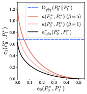
(a) $\lambda(P_{0},P_{1})\equiv\lambda_{0}$

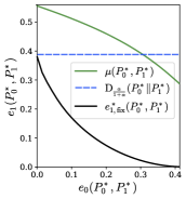
(b) $\textstyle\lambda(P_{0},P_{1})=\xi\mathrm{D}_{\frac{\beta}{1+\beta}}\mkern-1.5mu\left(P_{1}\middle\|P_{0}\right)$

Figure 1: The optimal type-II error exponent under different choices of $\lambda(P_{0},P_{1})$. Fix $\mathcal{X}=\{0,1\}$, $\varepsilon=0.01$, and choose $P_{0}^{*}=[0.6,0.4]$, $P_{1}^{*}=[0.1,0,9]$. In Figure 1(a), $\alpha=2$ and $\lambda_{0}$ increases from $0.001$ to $\mathrm{GJS}\mkern-1.5mu\left(P_{0}^{*},P_{1}^{*},\alpha\right)$ to obtain a curve. Note that $\kappa(P_{0}^{*},P_{1}^{*})$ is plot under two different $\beta$, whereas $e_{1,\mathrm{fix}}^{*}(P_{0}^{*},P_{1}^{*})$ and $\mathrm{D}_{\frac{\alpha}{1+\alpha}}\mkern-1.5mu\left(P_{0}^{*}\middle\|P_{1}^{*}\right)$ are independent of $\beta$. In Figure 1(b), $\alpha=\beta=0.7$ and $\xi$ increases from $0.001$ to $0.999$.

In Figure 1(a), there is still a trade-off between the two error exponents for sequential tests, and the benefit of sequentiality is more significant when $\beta$ is larger. This can also be observed analytically. When $\lambda(P_{0},P_{1})\equiv\lambda_{0}$, it can be shown that

$$e_{1,\mathrm{fix}}^{*}(P_{0},P_{1})=\inf_{\begin{subarray}{c}Q,Q_{0}\in\mathcal{P}(\mathcal{X})\\ \mathrm{GJS}\mkern-1.5mu\left(Q_{0},Q,\alpha\right)<\lambda_{0}\end{subarray}}\mathrm{D}\mkern-1.5mu\left(Q\middle\|P_{1}\right)+\alpha\mathrm{D}\mkern-1.5mu\left(Q_{0}\middle\|P_{0}\right),$$

$$\kappa(P_{0},P_{1})=\inf_{\begin{subarray}{c}Q_{0},Q_{1}\in\mathcal{P}(\mathcal{X})\\ \mathrm{GJS}\mkern-1.5mu\left(Q_{0},Q_{1},\alpha\right)<\lambda_{0}\end{subarray}}(1+\beta)\mathrm{D}\mkern-1.5mu\left(Q_{1}\middle\|P_{1}\right)+\alpha\mathrm{D}\mkern-1.5mu\left(Q_{0}\middle\|P_{0}\right).$$

Observe that they have the same form, with coefficient $1$ replaced by $1+\beta$. As a result, unlike in the fixed-length setup, the training sequence $T_{1}$ can improve the error exponent in sequential setups. This is interesting because the benefit occurs even in the semi-sequential setup, where $T_{1}$ has fixed length.

III-B Efficient Tests

Following [7, 8], we consider a special class of tests. A sequence of tests is said to be efficient [7] or universally exponentially consistent [12] if the error probabilities decay to zero exponentially for all the underlying distributions as the number of samples goes to infinity. The formal definition is provided under our problem formulation. Note that similar results were given in the preliminary version [11].

Definition 1 (Efficient Tests)

Given $\lambda:\mathcal{D}_{\varepsilon}\to(0,\infty)$ and let $\{\Phi_{n}\}$ be a sequence of tests such that for any underlying distributions $(P_{0},P_{1})\in\mathcal{D}_{\varepsilon}$,

• for each $\Phi_{n}=(\tau_{n},\delta_{n})$, $\mathbb{E}_{\theta}[\tau_{n}|P_{0},P_{1}]\leq n\ \forall\,\theta\in\{0,1\}$,

• $e_{0}(P_{0},P_{1})\geq\lambda(P_{0},P_{1})$.

We say $\{\Phi_{n}\}$ is efficient if the type-II error exponent $e_{1}(P_{0},P_{1})>0$ for all $(P_{0},P_{1})\in\mathcal{D}_{\varepsilon}$.

In order to have tests satisfying the universality constraints and being efficient, the constraint function $\lambda$ has to satisfy certain conditions, which leads to further simplification of the optimal error exponents, as shown below.

Proposition 2

Given $\lambda:\mathcal{D}_{\varepsilon}\to(0,\infty)$, if there exists a sequence of tests satisfying the universality constraints on the expected stopping time and the type-I error exponent, furthermore being efficient; then for all $(P_{0},P_{1})\in\mathcal{D}_{\varepsilon}$, $\lambda(P_{0},P_{1})\leq\mathrm{D}_{\frac{\beta}{1+\beta}}\mkern-1.5mu\left(P_{1}\middle\|P_{0}\right)$, and hence $\kappa(P_{0},P_{1})=\infty$. Thus

$$e_{1,\mathrm{semi}}^{*}(P_{0},P_{1}) =\min\left\{\mathrm{D}_{\frac{\alpha}{1+\alpha}}\mkern-1.5mu\left(P_{0}\middle\|P_{1}\right),\ \mu(P_{0},P_{1})\right\},$$

$$e_{1,\mathrm{seq}}^{*}(P_{0},P_{1}) =\mathrm{D}_{\frac{\alpha}{1+\alpha}}\mkern-1.5mu\left(P_{0}\middle\|P_{1}\right).$$

Following the proof in [8], it can be shown that the error exponents of efficient tests are upper bounded by the Rényi divergence, which imposes upper bounds on $\lambda(P_{0},P_{1})$. As a result, $g_{1}(Q_{1},Q_{0},Q_{1})\geq 0$ for all $(Q_{0},Q_{1})\in\mathcal{D}_{\varepsilon}$, and hence $\kappa(P_{0},P_{1})=\infty$. Detailed proof is provided in Appendix A-B.

Figure 1(b) demonstrates a special class of $\lambda$ that permits efficient tests. As shown in [7], there is a trade-off between the type-I and type-II error exponents of fixed-length tests. Proposition 2 implies that fully-sequential tests completely eradicate the trade-off, consistent with the result in [8]. Given the parameters in Figure 1(b), there is a trade-off for semi-sequential tests. Finally, we provide a necessary and sufficient condition on $\alpha$ and $\beta$ such that semi-sequential tests can achieve the same error exponents as fully-sequential tests.

Proposition 3

Let $\lambda(P_{0},P_{1})=\mathrm{D}_{\frac{\beta}{1+\beta}}\mkern-1.5mu\left(P_{1}\middle\|P_{0}\right)$ for all $(P_{0},P_{1})\in\mathcal{D}_{\varepsilon}$, then (1) holds if and only if $\alpha\beta\geq 1$.

$$\mathrm{D}_{\frac{\alpha}{1+\alpha}}\mkern-1.5mu\left(P_{0}\middle\|P_{1}\right)\leq\mu(P_{0},P_{1})\quad\forall\,(P_{0},P_{1})\in\mathcal{D}_{\varepsilon}$$ (1)

The proof can be found in Appendix A-C. Proposition 3 implies that if $\alpha\beta\geq 1$, then semi-sequential tests and fully-sequential tests can both achieve the optimal error exponents of efficient tests $(\mathrm{D}_{\frac{\beta}{1+\beta}}\mkern-1.5mu\left(P_{1}\middle\|P_{0}\right),\mathrm{D}_{\frac{\alpha}{1+\alpha}}\mkern-1.5mu\left(P_{0}\middle\|P_{1}\right))$ for all $(P_{0},P_{1})\in\mathcal{D}_{\varepsilon}$. On the other hand, if $\alpha\beta<1$, then for any semi-sequential tests, there exists some distributions $(P_{0},P_{1})\in\mathcal{D}_{\varepsilon}$ such that the point $(\mathrm{D}_{\frac{\beta}{1+\beta}}\mkern-1.5mu\left(P_{1}\middle\|P_{0}\right),\mathrm{D}_{\frac{\alpha}{1+\alpha}}\mkern-1.5mu\left(P_{0}\middle\|P_{1}\right))$ is not achievable, and there remains a trade-off between the two error exponents.

IV Converse

Here we prove the upper bound on the type-II error exponent of semi-sequential tests in Theorem 1, starting by showing $e_{1}(P_{0},P_{1})\leq\mathrm{D}_{\frac{\alpha}{1+\alpha}}\mkern-1.5mu\left(P_{0}\middle\|P_{1}\right)$. Following the proof of converse in [8], the bound is obtained via standard arguments based on data processing inequality and the optional stopping theorem.

To show $e_{1}(P_{0},P_{1})\leq\kappa(P_{0},P_{1})$, observe that when $\theta=1$ and the underlying distributions are $(Q_{0},Q_{1})\in\mathcal{D}_{\varepsilon}$, the empirical distributions $(\hat{P}^{k},\hat{P}_{0},\hat{P}_{1})$ will be close to $(Q_{1},Q_{0},Q_{1})$ with high probability. So if the empirical distributions are close to $(Q_{1},Q_{0},Q_{1})$, the test must not stop too late in order to ensure $\mathbb{E}_{1}\left[\tau_{n}|Q_{0},Q_{1}\right]\leq n$. However, stopping around $n$, if $g_{1}(Q_{1},Q_{0},Q_{1})<0$, the test must output $0$ in order to satisfy the universality constraint on the type-I error exponent according to the fixed-length result [7]. This leads to upper bounds on the type-II error exponent.

Finally, the term $\mu(P_{0},P_{1})$ corresponds to the limitation imposed by the fixed-length training sequences. The bound is obtained by a reduction from a fixed-length composite hypothesis testing problem. Intuitively, if we are allowed to drop the constraint on the expected stopping time and take infinitely many testing samples, $P_{\theta}$ can be fully known. In this situation, consider the following equivalent problem. Suppose a distribution $P\in\mathcal{P}_{\varepsilon}$ is fixed and known. The decision maker observes two independent fixed-length sequences $T_{0}^{N},T_{1}^{M}$, where $N=\left\lceil\alpha n\right\rceil$, $M=\left\lceil\beta n\right\rceil$, and the objective is to decide between the following two hypotheses:

$$\mathcal{H}_{0}:T_{0,k}\overset{\text{i.i.d.}}{\sim}P,\ T_{1,k}\overset{\text{i.i.d.}}{\sim}\bar{P}\text{ for some }\bar{P}\in\mathcal{P}_{\varepsilon}\setminus\{P\}$$

$$\mathcal{H}_{1}:T_{1,k}\overset{\text{i.i.d.}}{\sim}P,\ T_{0,k}\overset{\text{i.i.d.}}{\sim}\bar{P}\text{ for some }\bar{P}\in\mathcal{P}_{\varepsilon}\setminus\{P\}$$

Notice that this is a fixed-length composite hypothesis testing problem. Given a sequence of semi-sequential tests $\{\Phi_{n}\}$, we can use it for this new problem. Specifically, generate the testing sequence using the knowledge of $P$. Along with the observed fixed-length sequences $T_{0}^{N},T_{1}^{M}$, the test $\Phi_{n}$ will output a decision. The above method gives a randomized test, yet theoretically it can be easily derandomized without affecting the exponential rate. One can observe a correspondence between the error probabilities of the two problems, and hence a correspondence between the exponential rates of error probabilities. Since $\{\Phi_{n}\}$ satisfies the universality constraints on the type-I error exponent, we can apply the result for composite hypothesis testing in [7] with some slight modifications and get the desired bound $e_{1}(P_{0},P_{1})\leq\mu(P_{0},P_{1})$.

For the fully-sequential setup in Theorem 2, we use similar arguments to show that $e_{1}(P_{0},P_{1})$ is upper bounded by the first two terms $\mathrm{D}_{\frac{\alpha}{1+\alpha}}\mkern-1.5mu\left(P_{0}\middle\|P_{1}\right)$ and $\kappa(P_{0},P_{1})$. The detailed proof of converse can be found in Appendix A-D.

V Achievability

For the semi-sequential setup, we propose a two-phase test. Now the decision maker has the flexibility to decide when to stop, so intuitively we would like to take more samples before making the decision. Nevertheless, the expected stopping time should not exceed $n$, meaning the probability of taking more samples should be kept small. First consider the empirical distributions at time $n-1$, namely, $(\hat{P}^{n-1},\hat{P}_{0},\hat{P}_{1})\in\mathcal{P}(\mathcal{X})^{3}$. Observe that with high probability, the empirical distributions are close to the true underlying distributions. Define two subsets of $\mathcal{P}(\mathcal{X})^{3}$, for $i=0,1$,

$$\Lambda_{i}^{n}=\Big{\{}(Q,Q_{0},Q_{1})\,\Big{|}\,$$

$$\inf_{(P_{0}^{\prime},P_{1}^{\prime})\in\mathcal{D}_{\varepsilon}}\mathrm{D}\mkern-1.5mu\left(Q\middle\|P_{i}^{\prime}\right)+\alpha\mathrm{D}\mkern-1.5mu\left(Q_{0}\middle\|P_{0}^{\prime}\right)+\beta\mathrm{D}\mkern-1.5mu\left(Q_{1}\middle\|P_{1}^{\prime}\right)<\eta_{n}\Big{\}},$$

where $\eta_{n}=\big{[}(d+2)\log n+d\log(\left\lceil\alpha n\right\rceil+1)+d\log(\left\lceil\beta n\right\rceil+1)\big{]}/(n-1)$ is a margin vanishing in $n$. By the method of types, the empirical distributions lie in these sets with high probability. Hence the universality constraint on the expected stopping time can be satisfied with the following stopping time

$$\tau_{n}=\begin{cases}n-1&\quad\text{if }(\hat{P}^{n-1},\hat{P}_{0},\hat{P}_{1})\in\Lambda_{0}^{n}\cup\Lambda_{1}^{n},\\ n^{2}&\quad\text{if }(\hat{P}^{n-1},\hat{P}_{0},\hat{P}_{1})\in\left(\Lambda_{0}^{n}\cup\Lambda_{1}^{n}\right)^{\mathrm{c}}.\end{cases}$$ (2)

To specify the decision rule, introduce the following two sets,

$$\Gamma_{0} =\big{\{}(Q_{1},Q_{0},Q_{1})\,\big{|}\,(Q_{0},Q_{1})\in\mathcal{D}_{\varepsilon},\ g_{1}(Q_{1},Q_{0},Q_{1})<0\big{\}},$$

$$\Gamma_{1} =\big{\{}(Q_{1},Q_{0},Q_{1})\,\big{|}\,(Q_{0},Q_{1})\in\mathcal{D}_{\varepsilon},\ g_{1}(Q_{1},Q_{0},Q_{1})\geq 0\big{\}}.$$

Note that $\Gamma_{0}$ consists of the distributions under ground truth $1$ that are “close enough” to some possible distributions $(P_{0}^{\prime},P_{0}^{\prime},P_{1}^{\prime})$ under ground truth $0$. For $i=0,1$, let

$$\mathcal{B}_{n}(\Gamma_{i})= \bigcup_{(Q_{1},Q_{0},Q_{1})\in\Gamma_{i}}\big{\{}(R,R_{0},R_{1})\,\big{|}\,$$

$$\quad\mathrm{D}\mkern-1.5mu\left(R\middle\|Q_{1}\right)+\alpha\mathrm{D}\mkern-1.5mu\left(R_{0}\middle\|Q_{0}\right)+\beta\mathrm{D}\mkern-1.5mu\left(R_{1}\middle\|Q_{1}\right)<\eta_{n}\big{\}}$$

be a subset of $\mathcal{P}(\mathcal{X})^{3}$ that slightly extends $\Gamma_{i}$. When $\tau_{n}=n-1$, let $\delta_{n}:(X^{n-1},T_{0}^{N},T_{1}^{M})\mapsto\hat{\theta}$, where

$$\hat{\theta}=\begin{cases}0\quad\text{if }(\hat{P}^{n-1},\hat{P}_{0},\hat{P}_{1})\in\Lambda_{0}^{n}\cup\mathcal{B}_{n}(\Gamma_{0}),\\ 1\quad\text{if }(\hat{P}^{n-1},\hat{P}_{0},\hat{P}_{1})\in\mathcal{B}_{n}(\Gamma_{1}).\end{cases}$$ (3)

Notice that $\mathcal{B}_{n}(\Gamma_{0})\cup\mathcal{B}_{n}(\Gamma_{1})=\Lambda_{1}^{n}$. Also, when $\lambda(P_{0},P_{1})\leq\mathrm{D}_{\frac{\beta}{1+\beta}}\mkern-1.5mu\left(P_{1}\middle\|P_{0}\right)$ for all $(P_{0},P_{1})\in\mathcal{D}_{\varepsilon}$, we have $\Gamma_{0}=\emptyset$ and the decision rule is similar to that in [8].

When $\tau_{n}=n^{2}$, we use the fixed-length test in [7] for $n^{2}$ testing samples and $N$ training samples with threshold function $\lambda_{n}(P_{0},P_{1})=\lambda(P_{0},P_{1})/n$. As a result, we can ensure that the type-I error probability is of the same order as when $\tau_{n}=n-1$. Specifically, the decision rules is

$$\delta_{n}(X^{n^{2}},T_{0}^{N},T_{1}^{M})=\begin{cases}0\quad\text{if }g_{n}(\hat{P}^{n^{2}},\hat{P}_{0},\hat{P}_{1})<0,\\ 1\quad\text{otherwise}.\end{cases}$$

Using the method of types, the proposed test can be shown to satisfy the universality constraint on the type-I error exponent. Furthermore, with some careful analysis, the exponential rate of type-II error probability when $\tau_{n}=n-1$ is $\min\{\mathrm{D}_{\frac{\alpha}{1+\alpha}}\mkern-1.5mu\left(P_{0}\middle\|P_{1}\right),\kappa(P_{0},P_{1})\}$, where the two terms correspond to decision regions $\Lambda_{0}^{n}$ and $\mathcal{B}_{n}(\Gamma_{0})$ in (3) respectively. The type-II error probability when $\tau_{n}=n^{2}$ is upper bounded by $(n^{2}+1)(N+1)^{d}(M+1)^{d}\times 2^{-n\mu_{n}(P_{0},P_{1})}$, where $\mu_{n}(P_{0},P_{1})=$

$$\inf_{\begin{subarray}{c}Q,Q_{0},Q_{1}\in\mathcal{P}(\mathcal{X})\\ g_{n}(Q,Q_{0},Q_{1})<0\end{subarray}}\Big{(}n\mathrm{D}\mkern-1.5mu\left(Q\middle\|P_{1}\right)+\alpha\mathrm{D}\mkern-1.5mu\left(Q_{0}\middle\|P_{0}\right)+\beta\mathrm{D}\mkern-1.5mu\left(Q_{1}\middle\|P_{1}\right)\Big{)}.$$

If $\lambda$ satisfies Assumption 1, then it can be shown that $\lim_{n\to\infty}\mu_{n}(P_{0},P_{1})=\mu(P_{0},P_{1})$. Combining the above results, the type-II error exponent achieves $e_{1,\mathrm{semi}}^{*}(P_{0},P_{1})$.

For the fully-sequential setup, we propose a similar test. Again consider the empirical distributions at time $n-1$ and use the same stopping rule (2). When $\tau_{n}=n-1$, define the decision rule $\delta_{n}:(X^{n-1},T_{0}^{N_{n-1}},T_{1}^{M_{n-1}})\mapsto\hat{\theta}$, where $\hat{\theta}$ is specified in (3). When $\tau_{n}=n^{2}$, we use the fixed-length test in [7] for $n^{2}$ testing samples and $N_{n^{2}}=\left\lceil\alpha n^{2}\right\rceil$, $M_{n^{2}}=\left\lceil\beta n^{2}\right\rceil$ training samples with threshold function $\xi\mathrm{D}_{\frac{\beta}{1+\beta}}\mkern-1.5mu\left(P_{1}\middle\|P_{0}\right)$ for some $0<\xi<1$. By the results in [7], the error probabilities when $\tau_{n}=n^{2}$ vanish exponentially in $n^{2}$, which do not contribute to the error exponents. Following similar proof for semi-sequential tests, the expected stopping time and error exponents resulting from the part $\tau_{n}=n-1$ can be obtained. The detailed proof of converse is given in Appendix A-E.

Appendix A Appendix

Notations

For a subset $S$ of a topological space, we use $\mathrm{cl}(S)$ to denote closure of $S$. Also, $o(1)$ is used to denote vanishing terms, and $\mathsf{poly}\mkern-1.5mu\left(n\right)$ means some polynomial in $n$.

A-A Proof of Proposition 1

When $\lambda(P_{0},P_{1})\equiv\lambda_{0}$, we have $\displaystyle g(Q_{0},Q_{1})=\inf_{P_{1}^{\prime}\in\mathcal{P}_{\varepsilon}\setminus\{P_{1}\}}\Big{(}\alpha\mathrm{D}\mkern-1.5mu\left(Q_{0}\middle\|P_{1}\right)+\beta\mathrm{D}\mkern-1.5mu\left(Q_{1}\middle\|P_{1}^{\prime}\right)-\lambda(P_{1},P_{1}^{\prime})\Big{)}\geq\alpha\mathrm{D}\mkern-1.5mu\left(Q_{0}\middle\|P_{1}\right)-\lambda_{0}$, and hence

$$\mu(P_{0},P_{1}) =\inf_{\begin{subarray}{c}Q_{0},Q_{1}\in\mathcal{P}(\mathcal{X})\\ g(Q_{0},Q_{1})<0\end{subarray}}\Big{(}\alpha\mathrm{D}\mkern-1.5mu\left(Q_{0}\middle\|P_{0}\right)+\beta\mathrm{D}\mkern-1.5mu\left(Q_{1}\middle\|P_{1}\right)\Big{)}\geq\inf_{\begin{subarray}{c}Q_{0}\in\mathcal{P}(\mathcal{X})\\ \alpha\mathrm{D}\mkern-1.5mu\left(Q_{0}\middle\|P_{1}\right)<\lambda_{0}\end{subarray}}\alpha\mathrm{D}\mkern-1.5mu\left(Q_{0}\middle\|P_{0}\right).$$ (4)

In fact the infimum in (4) is attainable by some $Q_{0}\in\mathcal{P}_{\varepsilon}$. Moreover,

$$\kappa(P_{0},P_{1}) =\inf_{\begin{subarray}{c}(Q_{0},Q_{1})\in\mathcal{D}_{\varepsilon}\\ g_{1}(Q_{1},Q_{0},Q_{1})<0\end{subarray}}\Big{(}\mathrm{D}\mkern-1.5mu\left(Q_{1}\middle\|P_{1}\right)+\alpha\mathrm{D}\mkern-1.5mu\left(Q_{0}\middle\|P_{0}\right)+\beta\mathrm{D}\mkern-1.5mu\left(Q_{1}\middle\|P_{1}\right)\Big{)}\leq\inf_{\begin{subarray}{c}Q_{0}\in\mathcal{P}_{\varepsilon}\setminus\{P_{1}\}\\ g_{1}(P_{1},Q_{0},P_{1})<0\end{subarray}}\alpha\mathrm{D}\mkern-1.5mu\left(Q_{0}\middle\|P_{0}\right),$$ (5)

and $\displaystyle g_{1}(P_{1},Q_{0},P_{1})=\inf_{(P_{0}^{\prime},P_{1}^{\prime})\in\mathcal{D}_{\varepsilon}}\Big{(}\mathrm{D}\mkern-1.5mu\left(P_{1}\middle\|P_{0}^{\prime}\right)+\alpha\mathrm{D}\mkern-1.5mu\left(Q_{0}\middle\|P_{0}^{\prime}\right)+\beta\mathrm{D}\mkern-1.5mu\left(P_{1}\middle\|P_{1}^{\prime}\right)\Big{)}-\lambda_{0}\leq\alpha\mathrm{D}\mkern-1.5mu\left(Q_{0}\middle\|P_{1}\right)-\lambda_{0}$. The proof is complete by observing that (5) is upper bounded by (4).

A-B Proof of Proposition 2

Following the proof of converse in [8], we can obtain $\lambda(P_{0},P_{1})\leq e_{0}(P_{0},P_{1})\leq\mathrm{D}_{\frac{\beta}{1+\beta}}\mkern-1.5mu\left(P_{1}\middle\|P_{0}\right)$, where the first inequality follows from the universality constraint on the type-I error exponent. Then for $(Q_{0},Q_{1})\in\mathcal{D}_{\varepsilon}$,

$$g_{1}(Q_{1},Q_{0},Q_{1}) =\inf_{(P_{0}^{\prime},P_{1}^{\prime})\in\mathcal{D}_{\varepsilon}}\Big{(}\mathrm{D}\mkern-1.5mu\left(Q_{1}\middle\|P_{0}^{\prime}\right)+\alpha\mathrm{D}\mkern-1.5mu\left(Q_{0}\middle\|P_{0}^{\prime}\right)+\beta\mathrm{D}\mkern-1.5mu\left(Q_{1}\middle\|P_{1}^{\prime}\right)-\lambda(P_{0}^{\prime},P_{1}^{\prime})\Big{)}$$

$$\geq\inf_{(P_{0}^{\prime},P_{1}^{\prime})\in\mathcal{D}_{\varepsilon}}\Big{(}\mathrm{D}\mkern-1.5mu\left(Q_{1}\middle\|P_{0}^{\prime}\right)+\alpha\mathrm{D}\mkern-1.5mu\left(Q_{0}\middle\|P_{0}^{\prime}\right)+\beta\mathrm{D}\mkern-1.5mu\left(Q_{1}\middle\|P_{1}^{\prime}\right)-\mathrm{D}_{\frac{\beta}{1+\beta}}\mkern-1.5mu\left(P_{1}^{\prime}\middle\|P_{0}^{\prime}\right)\Big{)}$$

$$\geq\inf_{(P_{0}^{\prime},P_{1}^{\prime})\in\mathcal{D}_{\varepsilon}}\alpha\mathrm{D}\mkern-1.5mu\left(Q_{0}\middle\|P_{0}^{\prime}\right)\geq 0$$

The last line follows from the fact that Rényi divergence can be written as a minimization problem. We then have $\kappa(P_{0},P_{1})=\infty$ as it is the infimum of an empty set.

A-C Proof of Proposition 3

First we show that when $\alpha\beta\geq 1$, $\mu(P_{0},P_{1})\geq\mathrm{D}_{\frac{\alpha}{1+\alpha}}\mkern-1.5mu\left(P_{0}\middle\|P_{1}\right)$. Now $\lambda(P_{0},P_{1})=\mathrm{D}_{\frac{\beta}{1+\beta}}\mkern-1.5mu\left(P_{1}\middle\|P_{0}\right)$ for all $(P_{0},P_{1})\in\mathcal{D}_{\varepsilon}$. Hence it is equivalent to show that if for some $Q_{0},Q_{1}\in\mathcal{P}(\mathcal{X})$,

$$\alpha\mathrm{D}\mkern-1.5mu\left(Q_{0}\middle\|P_{0}\right)+\beta\mathrm{D}\mkern-1.5mu\left(Q_{1}\middle\|P_{1}\right)<\mathrm{D}_{\frac{\alpha}{1+\alpha}}\mkern-1.5mu\left(P_{0}\middle\|P_{1}\right),$$ (6)

then for all $P_{1}^{\prime}\in\mathcal{P}_{\varepsilon}\setminus\{P_{1}\}$, we have $\alpha\mathrm{D}\mkern-1.5mu\left(Q_{0}\middle\|P_{1}\right)+\beta\mathrm{D}\mkern-1.5mu\left(Q_{1}\middle\|P_{1}^{\prime}\right)\geq\mathrm{D}_{\frac{\beta}{1+\beta}}\mkern-1.5mu\left(P_{1}^{\prime}\middle\|P_{1}\right)$. Since the Rényi divergence can be written as a minimization problem, we upper bound the RHS of (6) by $\mathrm{D}\mkern-1.5mu\left(Q_{0}\middle\|P_{1}\right)+\alpha\mathrm{D}\mkern-1.5mu\left(Q_{0}\middle\|P_{0}\right)$ and get $\beta\mathrm{D}\mkern-1.5mu\left(Q_{1}\middle\|P_{1}\right)<\mathrm{D}\mkern-1.5mu\left(Q_{0}\middle\|P_{1}\right)$. For all $P_{1}^{\prime}\in\mathcal{P}_{\varepsilon}\setminus\{P_{1}\}$,

$$\alpha\mathrm{D}\mkern-1.5mu\left(Q_{0}\middle\|P_{1}\right)+\beta\mathrm{D}\mkern-1.5mu\left(Q_{1}\middle\|P_{1}^{\prime}\right)\geq\alpha\beta\mathrm{D}\mkern-1.5mu\left(Q_{1}\middle\|P_{1}\right)+\beta\mathrm{D}\mkern-1.5mu\left(Q_{1}\middle\|P_{1}^{\prime}\right)\geq\mathrm{D}\mkern-1.5mu\left(Q_{1}\middle\|P_{1}\right)+\beta\mathrm{D}\mkern-1.5mu\left(Q_{1}\middle\|P_{1}^{\prime}\right)\geq\mathrm{D}_{\frac{\beta}{1+\beta}}\mkern-1.5mu\left(P_{1}^{\prime}\middle\|P_{1}\right).$$

Second, we prove that when $\alpha\beta<1$, there exists $(P_{0},P_{1})\in\mathcal{D}_{\varepsilon}$ such that $\mu(P_{0},P_{1})<\mathrm{D}_{\frac{\alpha}{1+\alpha}}\mkern-1.5mu\left(P_{0}\middle\|P_{1}\right)$. Specifically, we want to find $P_{1}\in\mathcal{P}_{\varepsilon}$, $P_{0},P_{1}^{\prime}\in\mathcal{P}_{\varepsilon}\setminus\{P_{1}\}$, and $Q_{0},Q_{1}\in\mathcal{P}(\mathcal{X})$ such that

$$g(Q_{0},Q_{1}) \leq\alpha\mathrm{D}\mkern-1.5mu\left(Q_{0}\middle\|P_{1}\right)+\beta\mathrm{D}\mkern-1.5mu\left(Q_{1}\middle\|P_{1}^{\prime}\right)-\beta\mathrm{D}\mkern-1.5mu\left(V_{\beta}\middle\|P_{1}^{\prime}\right)-\mathrm{D}\mkern-1.5mu\left(V_{\beta}\middle\|P_{1}\right)<0,$$

$$\mu(P_{0},P_{1}) =\alpha\mathrm{D}\mkern-1.5mu\left(Q_{0}\middle\|P_{0}\right)+\beta\mathrm{D}\mkern-1.5mu\left(Q_{1}\middle\|P_{1}\right)<\alpha\mathrm{D}\mkern-1.5mu\left(V_{\alpha}\middle\|P_{0}\right)+\mathrm{D}\mkern-1.5mu\left(V_{\alpha}\middle\|P_{1}\right),$$

where $V_{\alpha}=\mathop{\mathrm{argmin}}_{V\in\mathcal{P}(\mathcal{X})}\left\{\alpha\mathrm{D}\mkern-1.5mu\left(V\middle\|P_{0}\right)+\mathrm{D}\mkern-1.5mu\left(V\middle\|P_{1}\right)\right\}$ and $V_{\beta}=\mathop{\mathrm{argmin}}_{V\in\mathcal{P}(\mathcal{X})}\left\{\beta\mathrm{D}\mkern-1.5mu\left(V\middle\|P_{1}^{\prime}\right)+\mathrm{D}\mkern-1.5mu\left(V\middle\|P_{1}\right)\right\}$. Take $Q_{0}=V_{\alpha}$ and $Q_{1}=V_{\beta}$, then it suffices to have $\alpha\mathrm{D}\mkern-1.5mu\left(V_{\alpha}\middle\|P_{1}\right)<\mathrm{D}\mkern-1.5mu\left(V_{\beta}\middle\|P_{1}\right)$ and $\beta\mathrm{D}\mkern-1.5mu\left(V_{\beta}\middle\|P_{1}\right)<\mathrm{D}\mkern-1.5mu\left(V_{\alpha}\middle\|P_{1}\right)$. Observe that $(P_{0},\alpha)$ and $(P_{1}^{\prime},\beta)$ play symmetric roles. WLOG assume $\alpha\leq\beta$ and get $\alpha<1$. Arbitrarily pick $(P_{0},P_{1})\in\mathcal{D}_{\varepsilon}$, and now the goal is to find $P_{1}^{\prime}\in\mathcal{P}_{\varepsilon}\setminus\{P_{1}\}$ such that $\alpha\mathrm{D}\mkern-1.5mu\left(V_{\alpha}\middle\|P_{1}\right)<\mathrm{D}\mkern-1.5mu\left(V_{\beta}\middle\|P_{1}\right)<\frac{1}{\beta}\mathrm{D}\mkern-1.5mu\left(V_{\alpha}\middle\|P_{1}\right)$. This is possible since $\alpha<\frac{1}{\beta}$ and $V_{\alpha}\neq P_{1}$. The closed-form expression of $V_{\beta}$ can be derived and notice that it is continuous in $P_{1}^{\prime}$. Hence $\mathrm{D}\mkern-1.5mu\left(V_{\beta}\middle\|P_{1}\right)$ is continuous in $P_{1}^{\prime}$. When $P_{1}^{\prime}=P_{1}$, $\mathrm{D}\mkern-1.5mu\left(V_{\beta}\middle\|P_{1}\right)=0$. When $P_{1}^{\prime}=P_{0}$, since $\alpha\leq\beta$, it can be shown that $\mathrm{D}\mkern-1.5mu\left(V_{\alpha}\middle\|P_{1}\right)\leq\mathrm{D}\mkern-1.5mu\left(V_{\beta}\middle\|P_{1}\right)$. By the intermediate value theorem, there exists $P_{1}^{\prime}$ between $P_{1}$ and $P_{0}$ with the desired property.

A-D Proof of Converse

A-D1 $\mathrm{D}_{\frac{\alpha}{1+\alpha}}\mkern-1.5mu\left(P_{0}\middle\|P_{1}\right)$

The proof for the fully-sequential setup is exactly the same as the proof of converse in [8]; whereas in the semi-sequential setup, replace the expected number of training samples $\mathbb{E}_{\theta}[N_{\tau}]$ by the deterministic $N$, $M$.

A-D2 $\kappa(P_{0},P_{1})$

Take $(Q_{0},Q_{1})\in\mathcal{D}_{\varepsilon}$ with $g_{1}(Q_{1},Q_{0},Q_{1})<0$. If there are no such $(Q_{0},Q_{1})$, then $\kappa(P_{0},P_{1})$ is infinity and we are done. Otherwise by definition, there exist some $(P_{0}^{\prime},P_{1}^{\prime})\in\mathcal{D}_{\varepsilon}$ such that $\mathrm{D}\mkern-1.5mu\left(Q\middle\|P_{0}^{\prime}\right)+\alpha\mathrm{D}\mkern-1.5mu\left(Q_{0}\middle\|P_{0}^{\prime}\right)+\beta\mathrm{D}\mkern-1.5mu\left(Q_{1}\middle\|P_{1}^{\prime}\right)<\lambda(P_{0}^{\prime},P_{1}^{\prime})$. Given $\epsilon>0$, define

$$\mathcal{B}_{\epsilon}(\bm{Q}) =\Big{\{}(R,R_{0},R_{1})\,\Big{|}\,\mathrm{D}\mkern-1.5mu\left(R\middle\|Q_{1}\right)+\alpha\mathrm{D}\mkern-1.5mu\left(R_{0}\middle\|Q_{0}\right)+\beta\mathrm{D}\mkern-1.5mu\left(R_{1}\middle\|Q_{1}\right)<\epsilon\Big{\}},$$

$$\mathcal{B}_{\lambda}(\bm{P}^{\prime}) =\Big{\{}(R,R_{0},R_{1})\,\Big{|}\,\mathrm{D}\mkern-1.5mu\left(R\middle\|P_{0}^{\prime}\right)+\alpha\mathrm{D}\mkern-1.5mu\left(R_{0}\middle\|P_{0}^{\prime}\right)+\beta\mathrm{D}\mkern-1.5mu\left(R_{1}\middle\|P_{1}^{\prime}\right)<(1-\epsilon)\lambda(P_{0}^{\prime},P_{1}^{\prime})\Big{\}}.$$

By the choice of $(P_{0}^{\prime},P_{1}^{\prime})$, we can take $\epsilon$ small enough such that $\mathcal{B}_{\epsilon}(\bm{Q})\subseteq\mathcal{B}_{\lambda}(\bm{P}^{\prime})$. For each semi-sequential test $\Phi_{n}=(\tau_{n},\delta_{n})$, by assumption $\mathbb{E}_{1}\left[\tau_{n}|Q_{0},Q_{1}\right]\leq n$. Thus by Markov’s inequality,

$$\mathbb{Q}_{1}\{\tau_{n}>n\}=\mathbb{Q}_{1}\{\tau_{n}\geq n+1\}\leq\frac{\mathbb{E}_{1}\left[\tau_{n}|Q_{0},Q_{1}\right]}{n+1}\leq\frac{n}{n+1}.$$ (7)

Now look at the empirical distributions at time $n$. Note that even if the test stops earlier, we can still consider the samples until $n$. By the method of types,

$$\mathbb{Q}_{1}\left\{(\hat{P}^{n},\hat{P}_{0}^{N},\hat{P}_{1}^{M})\notin\mathcal{B}_{\epsilon}(\bm{Q})\right\} \leq\sum_{(\hat{P}^{n},\hat{P}_{0}^{N},\hat{P}_{1}^{M})\in\left(\mathcal{P}_{d}^{n}\times\mathcal{P}_{d}^{N}\times\mathcal{P}_{d}^{M}\right)\cap\mathcal{B}_{\epsilon}(\bm{Q})^{\mathrm{c}}}2^{-\left(n\mathrm{D}\mkern-1.5mu\left(\hat{P}^{n}\middle\|Q_{1}\right)+N\mathrm{D}\mkern-1.5mu\left(\hat{P}_{0}^{N}\middle\|Q_{0}\right)+M\mathrm{D}\mkern-1.5mu\left(\hat{P}_{1}^{M}\middle\|Q_{1}\right)\right)}$$

$$\leq\sum_{(\hat{P}^{n},\hat{P}_{0}^{N},\hat{P}_{1}^{M})\in\left(\mathcal{P}_{d}^{n}\times\mathcal{P}_{d}^{N}\times\mathcal{P}_{d}^{M}\right)\cap\mathcal{B}_{\epsilon}(\bm{Q})^{\mathrm{c}}}2^{-n\left(\mathrm{D}\mkern-1.5mu\left(\hat{P}^{n}\middle\|Q_{1}\right)+\alpha\mathrm{D}\mkern-1.5mu\left(\hat{P}_{0}^{N}\middle\|Q_{0}\right)+\beta\mathrm{D}\mkern-1.5mu\left(\hat{P}_{1}^{M}\middle\|Q_{1}\right)\right)}$$

$$\leq\mathsf{poly}\mkern-1.5mu\left(n\right)2^{-n\epsilon}.$$ (8)

Combine (7) and (8), then for all $n$ large enough,

$$\mathbb{Q}_{1}\left\{(\hat{P}^{n},\hat{P}_{0}^{N},\hat{P}_{1}^{M})\in\mathcal{B}_{\epsilon}(\bm{Q})\text{ and }\tau_{n}\leq n\right\}\geq 1-\frac{n}{n+1}-\mathsf{poly}\mkern-1.5mu\left(n\right)2^{-n\epsilon}\geq\frac{1}{\mathsf{poly}\mkern-1.5mu\left(n\right)}.$$

Hence for all $n$ large enough, there exist some empirical distributions $(P^{n},P_{0}^{n},P_{1}^{n})\in\left(\mathcal{P}_{d}^{n}\times\mathcal{P}_{d}^{N}\times\mathcal{P}_{d}^{M}\right)\cap\mathcal{B}_{\epsilon}(\bm{Q})$ such that

$$\mathbb{Q}_{1}\left\{\tau_{n}\leq n\,\middle|\,(\hat{P}^{n},\hat{P}_{0}^{N},\hat{P}_{1}^{M})=(P^{n},P_{0}^{n},P_{1}^{n})\right\}\geq\frac{1}{\mathsf{poly}\mkern-1.5mu\left(n\right)}.$$ (9)

Since all the sequences in a given type class have the same probability, a key observation is that this conditional probability is independent of the underlying distributions and ground truth $\theta$. So now we consider the situation where the underlying distributions are $(P_{0}^{\prime},P_{1}^{\prime})$ and $\theta=0$. By the method of types and the fact that $(P^{n},P_{0}^{n},P_{1}^{n})\in\mathcal{B}_{\epsilon}(\bm{Q})\subseteq\mathcal{B}_{\lambda}(\bm{P}^{\prime})$, for $n$ large enough,

$$\mathbb{P}_{0}^{\prime}\left\{(\hat{P}^{n},\hat{P}_{0}^{N},\hat{P}_{1}^{M})=(P^{n},P_{0}^{n},P_{1}^{n})\right\} \geq\frac{1}{\mathsf{poly}\mkern-1.5mu\left(n\right)}2^{-\left(n\mathrm{D}\mkern-1.5mu\left(P^{n}\middle\|P_{0}^{\prime}\right)+N\mathrm{D}\mkern-1.5mu\left(P_{0}^{n}\middle\|P_{0}^{\prime}\right)+M\mathrm{D}\mkern-1.5mu\left(P_{1}^{n}\middle\|P_{1}^{\prime}\right)\right)}\geq\frac{1}{\mathsf{poly}\mkern-1.5mu\left(n\right)}2^{-n(1-\epsilon)\lambda(P_{0}^{\prime},P_{1}^{\prime})}$$ (10)

Using the key observation and the inequalities (9), (10), we know that for $n$ large enough

$$\mathbb{P}_{0}^{\prime}\left\{(\hat{P}^{n},\hat{P}_{0}^{N},\hat{P}_{1}^{M})=(P^{n},P_{0}^{n},P_{1}^{n})\text{ and }\tau_{n}\leq n\right\}\geq\frac{1}{\mathsf{poly}\mkern-1.5mu\left(n\right)}2^{-n(1-\epsilon)\lambda(P_{0}^{\prime},P_{1}^{\prime})}.$$

Consider the type-I error probability

$$\pi_{0}(\Phi_{n}|P_{0}^{\prime},P_{1}^{\prime}) \geq\mathbb{P}_{0}^{\prime}\left\{\hat{\theta}=1,\,(\hat{P}^{n},\hat{P}_{0}^{N},\hat{P}_{1}^{M})=(P^{n},P_{0}^{n},P_{1}^{n})\text{ and }\tau_{n}\leq n\right\}$$

$$\geq\frac{1}{\mathsf{poly}\mkern-1.5mu\left(n\right)}2^{-n(1-\epsilon)\lambda(P_{0}^{\prime},P_{1}^{\prime})}\times\mathbb{P}_{0}^{\prime}\left\{\hat{\theta}=1\,\middle|\,(\hat{P}^{n},\hat{P}_{0}^{N},\hat{P}_{1}^{M})=(P^{n},P_{0}^{n},P_{1}^{n})\text{ and }\tau_{n}\leq n\right\}.$$

Since $\{\Phi_{n}\}$ satisfies the constraint on the type-I error exponent, that is $\pi_{0}(\Phi_{n}|P_{0}^{\prime},P_{1}^{\prime})\mathrel{\dot{\leq}}2^{-n\lambda(P_{0}^{\prime},P_{1}^{\prime})}$, we must have

$$\mathbb{P}_{0}^{\prime}\left\{\hat{\theta}=1\,\middle|\,(\hat{P}^{n},\hat{P}_{0}^{N},\hat{P}_{1}^{M})=(P^{n},P_{0}^{n},P_{1}^{n})\text{ and }\tau_{n}\leq n\right\}=o(1).$$ (11)

Again, since all the sequences in a given type class have the same probability, the above conditional probability is independent of the underlying distributions and ground truth $\theta$. When the underlying distributions are $(P_{0},P_{1})$ and $\theta=1$, the error probability can be lower bounded using (9), (11) and the method of types. Specifically, for $n$ large enough,

$$\pi_{1}(\Phi_{n}|P_{0},P_{1}) \geq\mathbb{P}_{1}\left\{\hat{\theta}=0,\,(\hat{P}^{n},\hat{P}_{0}^{N},\hat{P}_{1}^{M})=(P^{n},P_{0}^{n},P_{1}^{n})\text{ and }\tau_{n}\leq n\right\}\geq\frac{1}{\mathsf{poly}\mkern-1.5mu\left(n\right)}2^{-n\big{(}\mathrm{D}\mkern-1.5mu\left(P^{n}\middle\|P_{1}\right)+\alpha\mathrm{D}\mkern-1.5mu\left(P_{0}^{n}\middle\|P_{0}\right)+\beta\mathrm{D}\mkern-1.5mu\left(P_{1}^{n}\middle\|P_{1}\right)\big{)}}.$$

Hence $e_{1}(P_{0},P_{1})\leq\liminf_{n\to\infty}\big{(}\mathrm{D}\mkern-1.5mu\left(P^{n}\middle\|P_{1}\right)+\alpha\mathrm{D}\mkern-1.5mu\left(P_{0}^{n}\middle\|P_{0}\right)+\beta\mathrm{D}\mkern-1.5mu\left(P_{1}^{n}\middle\|P_{1}\right)\big{)}$. Let $(P^{\epsilon},P_{0}^{\epsilon},P_{1}^{\epsilon})$ be a limit point of $\{(P^{n},P_{0}^{n},P_{1}^{n})\}$, then by the continuity of KL divergence, $e_{1}(P_{0},P_{1})\leq\mathrm{D}\mkern-1.5mu\left(P^{\epsilon}\middle\|P_{1}\right)+\alpha\mathrm{D}\mkern-1.5mu\left(P_{0}^{\epsilon}\middle\|P_{0}\right)+\beta\mathrm{D}\mkern-1.5mu\left(P_{1}^{\epsilon}\middle\|P_{1}\right)$. Also by the continuity of KL divergence, $\mathrm{D}\mkern-1.5mu\left(P^{\epsilon}\middle\|Q_{1}\right)+\alpha\mathrm{D}\mkern-1.5mu\left(P_{0}^{\epsilon}\middle\|Q_{0}\right)+\beta\mathrm{D}\mkern-1.5mu\left(P_{1}^{\epsilon}\middle\|Q_{1}\right)\leq\epsilon$. As $\epsilon$ goes to $0$, $(P^{\epsilon},P_{0}^{\epsilon},P_{1}^{\epsilon})$ converge to $(Q_{1},Q_{0},Q_{1})$, and

$$e_{1}(P_{0},P_{1}) \leq\liminf_{\epsilon\to 0}\big{(}\mathrm{D}\mkern-1.5mu\left(P^{\epsilon}\middle\|P_{1}\right)+\alpha\mathrm{D}\mkern-1.5mu\left(P_{0}^{\epsilon}\middle\|P_{0}\right)+\beta\mathrm{D}\mkern-1.5mu\left(P_{1}^{\epsilon}\middle\|P_{1}\right)\big{)}=\mathrm{D}\mkern-1.5mu\left(Q_{1}\middle\|P_{1}\right)+\alpha\mathrm{D}\mkern-1.5mu\left(Q_{0}\middle\|P_{0}\right)+\beta\mathrm{D}\mkern-1.5mu\left(Q_{1}\middle\|P_{1}\right).$$

Since this hold for all $(Q_{0},Q_{1})\in\mathcal{D}_{\varepsilon}$ with $g_{1}(Q_{1},Q_{0},Q_{1})<0$, we get the desired result.

A-D3 $\mu(P_{0},P_{1})$

Here we state the result about composite hypothesis testing in [7] in a more general form. Specifically, instead of observing one sequence of length $n$, consider $s$ mutually independent sequences each with length linear in $n$. The formal problem formulation is given in the following.

Let $s\in\mathbb{N}$, and $\mathcal{X}_{1},\mathcal{X}_{2},\dots,\mathcal{X}_{s}$ be finite alphabets. The decision maker observes $s$ mutually independent sequences $X_{1}^{N_{1}},X_{2}^{N_{2}},\dots,X_{s}^{N_{s}}$, where $N_{i}\in\mathbb{N}$ is the length of the $i$-th sequence $X_{i}^{N_{i}}=(X_{i,1},X_{i,2},\dots,X_{i,N_{i}})\in\mathcal{X}_{i}^{N_{i}}$ for $i=1,2,\dots,s$. Given the unknown ground truth $\theta\in\{0,1\}$, each sequence $X_{i}^{N_{i}}$ i.i.d. follow $P_{\theta,i}$, for some $\bm{P}_{\theta}=(P_{\theta,1},P_{\theta,2},\dots,P_{\theta,s})\in\mathscr{P}_{\theta}$. Here $\mathscr{P}_{0},\mathscr{P}_{1}\subseteq\bm{\mathcal{P}}:=\mathcal{P}(\mathcal{X}_{1})\times\mathcal{P}(\mathcal{X}_{2})\times\dots\times\mathcal{P}(\mathcal{X}_{s})$ are the set of possible underlying distributions when the ground truth is $0$ and $1$, respectively. Note that if $|\mathscr{P}_{0}|=|\mathscr{P}_{1}|=1$, this reduces to the simple binary hypothesis problem.

The objective of the decision maker is to output $\hat{\theta}\in\{0,1\}$ as an estimation of the ground truth $\theta$, based on the observed samples. Let $n$ be an index of the problem and assume each $N_{i}$ grows linearly in $n$. Specifically, $\lim_{n\to\infty}\frac{N_{i}}{n}=\alpha_{i}>0$ for $i=1,2,\dots,s$. A test $\Phi_{n}$ is a function that maps observations $(X_{1}^{N_{1}},X_{2}^{N_{2}},\dots,X_{s}^{N_{s}})$ to $\hat{\theta}$. Given ground truth $\theta$ and underlying distributions $\bm{P}_{\theta}$, the error probability $\pi_{\theta}(\Phi_{n}|\bm{P}_{\theta})=\mathbb{P}_{\theta}\{\hat{\theta}\neq\theta\}$, where $\mathbb{P}_{\theta}$ is the shorthand notation for the joint probability law of all the sequences. The error exponent is defined as $e_{\theta}(\bm{P}_{\theta})=\liminf_{n\to\infty}-\frac{1}{n}\log\pi_{\theta}(\Phi_{n}|\bm{P}_{\theta})$.

Consider the competitive Neyman-Pearson criterion. The result is summarized in the following theorem.

Theorem 4 (Levitan and Merhav [7])

Let $\lambda:\mathscr{P}_{0}\to(0,\infty)$, and $\{\Phi_{n}\}$ be a sequence of tests such that the type-I error exponent satisfies $e_{0}(\bm{P}_{0})\geq\lambda(\bm{P}_{0})$ for all $\bm{P}_{0}\in\mathscr{P}_{0}$. Then for any $\bm{P}_{1}\in\mathscr{P}_{1}$,

$$e_{1}(\bm{P}_{1})\leq\inf_{\begin{subarray}{c}\bm{Q}\in\bm{\mathcal{P}}\\ g(\bm{Q})<0\end{subarray}}\sum_{i=1}^{s}\alpha_{i}\mathrm{D}\mkern-1.5mu\left(Q_{i}\middle\|P_{1,i}\right),$$ (12)

where $\bm{Q}$ denotes the tuple $(Q_{1},Q_{2},\dots,Q_{s})$, and $g(\bm{Q})=\inf_{\bm{P}_{0}^{\prime}\in\mathscr{P}_{0}}\Big{(}\sum_{i=1}^{s}\alpha_{i}\mathrm{D}\mkern-1.5mu\left(Q_{i}\middle\|P_{1,i}^{\prime}\right)-\lambda(\bm{P}_{0}^{\prime})\Big{)}$.

The proof involves some slight modifications to the original version in [7], details are omitted here.

Notice that the composite hypothesis testing problem mentioned in Section IV can be written in the above form. Specifically, take $s=2$, $\mathcal{X}_{1}=\mathcal{X}_{2}=\mathcal{X}$, $(\alpha_{1},\alpha_{2})=(\alpha,\beta)$, with the two sets of distributions being $\mathscr{P}_{0}=\left\{(P,\bar{P})\,\middle|\,(P,\bar{P})\in\mathcal{D}_{\varepsilon}\right\}$ and $\mathscr{P}_{1}=\left\{(\bar{P},P)\,\middle|\,(P,\bar{P})\in\mathcal{D}_{\varepsilon}\right\}$. The correspondence between the error probabilities mentioned in Section IV is specified as:

(original)(new problem)

$$\pi_{0}(\Phi_{n}|P_{0},P_{1})=\pi_{0}(\Phi_{n}|\bm{P}_{0}=(P_{0},P_{1}))\quad(P=P_{0}),$$

$$\pi_{1}(\Phi_{n}|P_{0},P_{1})=\pi_{1}(\Phi_{n}|\bm{P}_{1}=(P_{0},P_{1}))\quad(P=P_{1}).$$

Furthermore, the correspondence between the error exponents is $e_{0}(P_{0},P_{1})=e_{0}(\bm{P}_{0}=(P_{0},P_{1}))$ and $e_{1}(P_{0},P_{1})=e_{1}(\bm{P}_{1}=(P_{0},P_{1}))$. Since $\{\Phi_{n}\}$ satisfies the universality constraints on the type-I error exponent, for any fixed $P\in\mathcal{P}_{\varepsilon}$, we have $e_{0}(\bm{P}_{0}=(P,\bar{P}))=e_{0}(P,\bar{P})\geq\lambda(P,\bar{P})$ for all $\bm{P}_{0}=(P,\bar{P})\in\mathscr{P}_{0}$. By Theorem 4, for all $\bm{P}_{1}=(\bar{P},P)\in\mathscr{P}_{1}$

$$e_{1}(\bm{P}_{1}=(\bar{P},P))\leq\inf_{\begin{subarray}{c}Q_{0},Q_{1}\in\mathcal{P}(\mathcal{X})\\ g(Q_{0},Q_{1})<0\end{subarray}}\Big{(}\alpha\mathrm{D}\mkern-1.5mu\left(Q_{0}\middle\|\bar{P}\right)+\beta\mathrm{D}\mkern-1.5mu\left(Q_{1}\middle\|P\right)\Big{)},$$ (13)

where $\displaystyle g(Q_{0},Q_{1})=\inf_{\bm{P}_{0}=(P,\bar{P}^{\prime})\in\mathscr{P}_{0}}\Big{(}\alpha\mathrm{D}\mkern-1.5mu\left(Q_{0}\middle\|P\right)+\beta\mathrm{D}\mkern-1.5mu\left(Q_{1}\middle\|\bar{P}^{\prime}\right)-\lambda(P,\bar{P}^{\prime})\Big{)}$.

As the bound (13) holds for all $(P,\bar{P})\in\mathcal{D}_{\varepsilon}$, we can apply the correspondence between error exponents and change some variables to get the desired bound $e_{1}(P_{0},P_{1})\leq\mu(P_{0},P_{1})$.

A-E Proof of Achievability

A-E1 Semi-Sequential Setup

First we show that the proposed test satisfies the universality constraint on the expected stopping time. Given any $(P_{0},P_{1})\in\mathcal{D}_{\varepsilon}$ and $\theta\in\{0,1\}$, we have

$$\mathbb{E}_{\theta}[\tau_{n}] \leq n-1+\mathbb{P}_{\theta}\left\{(\hat{P}^{n-1},\hat{P}_{0},\hat{P}_{1})\in(\Lambda_{\theta}^{n})^{\mathrm{c}}\right\}\times n^{2}\leq n-1+n^{d}(N+1)^{d}(M+1)^{d}\times 2^{-(n-1)\eta_{n}}\times n^{2}=n,$$

where the last inequality follows from the method of types. To calculate the error exponents, we introduce a useful lemma and define some sets.

Lemma 1

Let $S\subseteq\mathbb{R}^{m}$ be a compact set, $f:S\to\mathbb{R}$ be a continuous function and $A\subseteq S$. Given $\epsilon>0$ and $x\in\mathbb{R}^{m}$, let $\mathcal{B}^{\prime}_{\epsilon}(x)=\left\{y\in\mathbb{R}^{m}:\|y-x\|<\epsilon\right\}$ be the $\epsilon$-ball centered at $x$. Let $\mathcal{B}^{\prime}_{\epsilon}(A)=\cup_{x\in A}\mathcal{B}^{\prime}_{\epsilon}(x)$. Then $\inf_{x\in A}f(x)=\inf_{x\in\mathrm{cl}(A)}f(x)$ and $\lim_{\epsilon\to 0}\inf_{x\in\mathcal{B}^{\prime}_{\epsilon}(A)\cap S}f(x)=\inf_{x\in\mathrm{cl}(A)}f(x)$.

The proof is easy and the details can be found in Appendix A-E3. Since the probability simplex $\mathcal{P}(\mathcal{X})^{3}$ can be embedded into $\mathbb{R}^{3(d-1)}$, consider for $i=0,1$,

$$\mathcal{B}^{\prime}_{n}(\Gamma_{i})=\bigcup_{(Q_{1},Q_{0},Q_{1})\in\Gamma_{i}}\Big{\{}(R,R_{0},R_{1})\in\mathcal{P}(\mathcal{X})^{3}\,\Big{|}\,\big{\|}(R,R_{0},R_{1})-(Q_{1},Q_{0},Q_{1})\big{\|}<c\eta_{n}\Big{\}}.$$

By Pinsker’s inequality and inequalities between 1-norm and 2-norm, we know that $\mathcal{B}_{n}(\Gamma_{i})\subseteq\mathcal{B}^{\prime}_{n}(\Gamma_{i})$ for some constant $c>0$.

For the type-I error exponent, based on the stopping time, the error events can be divided into two parts. When $\tau_{n}=n-1$, there is an error only if $(\hat{P}^{n-1},\hat{P}_{0},\hat{P}_{1})\in\mathcal{B}_{n}(\Gamma_{1})$. If $\Gamma_{1}\neq\emptyset$, using the method of types,

$$\mathbb{P}_{0}\left\{(\hat{P}^{n-1},\hat{P}_{0},\hat{P}_{1})\in\mathcal{B}_{n}(\Gamma_{1})\right\} \leq\mathbb{P}_{0}\left\{(\hat{P}^{n-1},\hat{P}_{0},\hat{P}_{1})\in\mathcal{B}^{\prime}_{n}(\Gamma_{1})\right\}\leq n^{d}(N+1)^{d}(M+1)^{d}\times 2^{-n\tilde{\lambda}_{n}(P_{0},P_{1})},$$

where $\displaystyle\tilde{\lambda}_{n}(P_{0},P_{1})=\inf_{(R,R_{0},R_{1})\in\mathcal{B}^{\prime}_{n}(\Gamma_{1})}\Big{(}\mathrm{D}\mkern-1.5mu\left(R\middle\|P_{0}\right)+\alpha\mathrm{D}\mkern-1.5mu\left(R_{0}\middle\|P_{0}\right)+\beta\mathrm{D}\mkern-1.5mu\left(R_{1}\middle\|P_{1}\right)\Big{)}$. Since $\eta_{n}$ vanishes as $n$ goes to infinity, using Lemma 1 and the definition of $\Gamma_{1}$,

$$\lim_{n\to\infty}\tilde{\lambda}_{n}(P_{0},P_{1})=\inf_{(R,R_{0},R_{1})\in\Gamma_{1}}\Big{(}\mathrm{D}\mkern-1.5mu\left(R\middle\|P_{0}\right)+\alpha\mathrm{D}\mkern-1.5mu\left(R_{0}\middle\|P_{0}\right)+\beta\mathrm{D}\mkern-1.5mu\left(R_{1}\middle\|P_{1}\right)\Big{)}\geq\lambda(P_{0},P_{1}).$$

When $\tau_{n}=n^{2}$, by the method of types,

$$\mathbb{P}_{0}\left\{\tau_{n}=n^{2},\ \hat{\theta}=1\right\}\leq(n^{2}+1)^{d}(N+1)^{d}(M+1)^{d}\times 2^{-n^{2}\lambda_{n}(P_{0},P_{1})}\doteq 2^{-n\lambda(P_{0},P_{1})}.$$

As a result, the type-I error probability has exponential rate $\lambda(P_{0},P_{1})$, which satisfies the universality constraint on the type-I error exponent.

For the type-II error exponent, when $\tau_{n}=n-1$, the error probability is upper bounded by

$$\quad\,\mathbb{P}_{1}\left\{(\hat{P}^{n-1},\hat{P}_{0},\hat{P}_{1})\in\Lambda_{0}^{n}\cup\mathcal{B}_{n}(\Gamma_{0})\right\}\leq\mathbb{P}_{1}\left\{(\hat{P}^{n-1},\hat{P}_{0},\hat{P}_{1})\in\Lambda_{0}^{n}\right\}+\mathbb{P}_{1}\left\{(\hat{P}^{n-1},\hat{P}_{0},\hat{P}_{1})\in\mathcal{B}^{\prime}_{n}(\Gamma_{0})\right\}$$ (14)

Since $\eta_{n}\to 0$ as $n\to\infty$, following the proof of error exponents in [8], $\mathbb{P}_{1}\left\{(\hat{P}^{n-1},\hat{P}_{0},\hat{P}_{1})\in\Lambda_{0}^{n}\right\}\mathrel{\dot{\leq}}2^{-n\mathrm{D}_{\frac{\alpha}{1+\alpha}}\mkern-1.5mu\left(P_{0}\middle\|P_{1}\right)}$. Also, if $\Gamma_{0}\neq\emptyset$ is not empty, then by the method of types,

$$\mathbb{P}_{1}\left\{(\hat{P}^{n-1},\hat{P}_{0},\hat{P}_{1})\in\mathcal{B}^{\prime}_{n}(\Gamma_{0})\right\}\leq n^{d}(N+1)^{d}(M+1)^{d}\times 2^{-n\kappa_{n}(P_{0},P_{1})},$$

where $\displaystyle\kappa_{n}(P_{0},P_{1})=\inf_{(R,R_{0},R_{1})\in\mathcal{B}^{\prime}_{n}(\Gamma_{0})}\Big{(}\mathrm{D}\mkern-1.5mu\left(R\middle\|P_{1}\right)+\alpha\mathrm{D}\mkern-1.5mu\left(R_{0}\middle\|P_{0}\right)+\beta\mathrm{D}\mkern-1.5mu\left(R_{1}\middle\|P_{1}\right)\Big{)}$. Since $\eta_{n}\to 0$ as $n\to\infty$, by Lemma 1,

$$\lim_{n\to\infty}\kappa_{n}(P_{0},P_{1})=\inf_{(R,R_{0},R_{1})\in\Gamma_{0}}\Big{(}\mathrm{D}\mkern-1.5mu\left(R\middle\|P_{0}\right)+\alpha\mathrm{D}\mkern-1.5mu\left(R_{0}\middle\|P_{0}\right)+\beta\mathrm{D}\mkern-1.5mu\left(R_{1}\middle\|P_{1}\right)\Big{)}=\kappa(P_{0},P_{1}).$$

Therefore, the exponential error rate when $\tau_{n}=n-1$ is $\min\{\mathrm{D}_{\frac{\alpha}{1+\alpha}}\mkern-1.5mu\left(P_{0}\middle\|P_{1}\right),\kappa(P_{0},P_{1})\}$. On the other hand, when $\tau_{n}=n^{2}$, it remains to show that $\lim_{n\to\infty}\mu_{n}(P_{0},P_{1})=\mu(P_{0},P_{1})$.

Lemma 2

For $(P_{0},P_{1})\in\mathcal{D}_{\varepsilon}$, the sequence $\{\mu_{n}(P_{0},P_{1})\}$ is non-decreasing in $n$, and if $\lambda$ satisfies Assumption 1, then $\lim_{n\to\infty}\mu_{n}(P_{0},P_{1})=\mu(P_{0},P_{1})$.

As $n$ grows, to minimize $n\mathrm{D}\mkern-1.5mu\left(Q\middle\|P_{1}\right)+\alpha\mathrm{D}\mkern-1.5mu\left(Q_{0}\middle\|P_{0}\right)+\beta\mathrm{D}\mkern-1.5mu\left(Q_{1}\middle\|P_{1}\right)$, $Q$ should be close to $P_{1}$, otherwise $n\mathrm{D}\mkern-1.5mu\left(Q\middle\|P_{1}\right)$ gets too large. Also, to have $g_{n}(Q,Q_{0},Q_{1})$ less than $0$, $P_{0}^{\prime}$ should be close to $Q$. Setting $P_{0}^{\prime}=Q=P_{1}$ gives $\mu(P_{0},P_{1})$. Note that in some steps, we utilize the compactness of $\mathcal{P}_{\varepsilon}$ and Assumption 1. By Lemma 2, the exponential error rate when $\tau_{n}=n^{2}$ is $\mu(P_{0},P_{1})$. Combining the above results, the type-II error exponent is shown to achieve the upper bound $e_{1,\mathrm{semi}}^{*}(P_{0},P_{1})$.

A-E2 Fully-Sequential Setup

We start by clearly define the decision rule when $\tau_{n}=n^{2}$. Specifically, let

$$\delta_{n}(X^{n^{2}},T_{0}^{N_{n^{2}}},T_{1}^{M_{n^{2}}})=\begin{cases}0\quad\text{if }\tilde{g}(\hat{P}^{n^{2}},\hat{P}_{0},\hat{P}_{1})<0,\\ 1\quad\text{otherwise},\end{cases}$$

where $\displaystyle\tilde{g}(Q,Q_{0},Q_{1})=\inf_{(P_{0}^{\prime},P_{1}^{\prime})\in\mathcal{D}_{\varepsilon}}\Big{(}\mathrm{D}\mkern-1.5mu\left(Q\middle\|P_{0}^{\prime}\right)+\alpha\mathrm{D}\mkern-1.5mu\left(Q_{0}\middle\|P_{0}^{\prime}\right)+\beta\mathrm{D}\mkern-1.5mu\left(Q_{1}\middle\|P_{1}^{\prime}\right)-\xi\mathrm{D}_{\frac{\beta}{1+\beta}}\mkern-1.5mu\left(P_{1}^{\prime}\middle\|P_{0}^{\prime}\right)\Big{)}$.

To show that the proposed test satisfies the universality constraint on the expected stopping time, just follow the same proof for semi-sequential tests. For the type-I error exponent, based on the stopping time, the error events can be divided into two parts. When $\tau_{n}=n-1$, using the same proof as for semi-sequential tests, the exponential rate of error probability is at least $\lambda(P_{0},P_{1})$. When $\tau_{n}=n^{2}$, by the method of types,

$$\quad\ \mathbb{P}_{0}\left\{\tau_{n}=n^{2},\ \delta_{n}(X^{n^{2}},T_{0}^{N_{n^{2}}},T_{1}^{M_{n^{2}}})=1\right\}\leq(n^{2}+1)^{d}(\left\lceil\alpha n^{2}\right\rceil+1)^{d}(\left\lceil\beta n^{2}\right\rceil+1)^{d}\times 2^{-n^{2}\xi\mathrm{D}_{\frac{\beta}{1+\beta}}\mkern-1.5mu\left(P_{1}\middle\|P_{0}\right)}\mathrel{\dot{\leq}}2^{-n\lambda(P_{0},P_{1})}.$$

Thus the error probability has exponential rate $\lambda(P_{0},P_{1})$, satisfying the universality constraint on the type-I error exponent.

For the type-II error exponent, when $\tau_{n}=n-1$, using the same proof as for semi-sequential tests, the exponential rate of error probability is $\min\{\mathrm{D}_{\frac{\alpha}{1+\alpha}}\mkern-1.5mu\left(P_{0}\middle\|P_{1}\right),\kappa(P_{0},P_{1})\}$. On the other hand, when $\tau_{n}=n^{2}$, by the results in [7], the error probabilities vanish exponentially in $n^{2}$, which do not contribute to the error exponents. Combining the above results, the type-II error exponent is shown to achieve the upper bound $e_{1,\mathrm{seq}}^{*}(P_{0},P_{1})$.

A-E3 Proof of Lemma 1

For the first part, clearly, $\inf_{x\in A}f(x)\geq\inf_{x\in\mathrm{cl}(A)}f(x)$. For $y\in\mathrm{cl}(A)$, choose a sequence $\{y_{n}\}$ such that $y_{n}\in A$ and $y_{n}\to y$. By the continuity of $f$ and the definition of infimum, we have $f(y)=\lim_{n\to\infty}f(y_{n})\geq\inf_{x\in A}f(x)$. Since this holds for all $y\in\mathrm{cl}(A)$, it follows that $\inf_{x\in\mathrm{cl}(A)}f(x)\geq\inf_{x\in A}f(x)$.

For the second part, observe that for any $\epsilon>0$, $\inf_{x\in\mathcal{B}^{\prime}_{\epsilon}(A)\cap S}f(x)\leq\inf_{x\in\mathrm{cl}(A)}f(x)<\infty$. Also, $\inf_{x\in\mathcal{B}^{\prime}_{\epsilon}(A)\cap S}f(x)$ is non-decreasing as $\epsilon\to 0$. Hence we know the limit exists. Assume $\lim_{\epsilon\to 0}\inf_{x\in\mathcal{B}^{\prime}_{\epsilon}(A)\cap S}f(x)=a<\inf_{x\in\mathrm{cl}(A)}f(x)$. For each $n\in\mathbb{N}$, there exists $y_{n}\in\mathcal{B}^{\prime}_{1/n}(A)\cap S$ such that $f(y_{n})\leq\inf_{x\in\mathcal{B}^{\prime}_{1/n}(A)\cap S}f(x)+1/n$. Since $y_{n}\in\mathcal{B}^{\prime}_{1/n}(A)$, there exists $x_{n}\in A$ such that $\left\lVert y_{n}-x_{n}\right\rVert\leq 1/n$. Consider a convergent subsequence $\{y_{n_{i}}\}$ and let $y\in S$ denote the limit point. Since $\left\lVert y-x_{n_{i}}\right\rVert\leq\left\lVert y-y_{n_{i}}\right\rVert+\left\lVert y_{n_{i}}-x_{n_{i}}\right\rVert$ converges to $0$ as $i$ goes to infinity, it follows that $y\in\mathrm{cl}(A)$. By the continuity of $f$, we have $f(y)=\lim_{i\to\infty}f(y_{n_{i}})\leq a<\inf_{x\in\mathrm{cl}(A)}f(x)$, which makes a contradiction.

A-E4 Proof of Lemma 2

First, $\mu(P_{0},P_{1})$ is clearly finite as we can take $Q_{1}\neq Q_{0}=P_{1}$ and hence $g(Q_{0},Q_{1})<0$. We then show that $\{\mu_{n}(P_{0},P_{1})\}$ is bounded above by $\mu(P_{0},P_{1})$. Choose $Q=P_{1}$ and restrict $P_{0}^{\prime}=P_{1}$ in $g_{n}(P_{1},Q_{0},Q_{1})$. We have

$$\mu_{n}(P_{0},P_{1})\leq\inf_{\begin{subarray}{c}Q_{0},Q_{1}\in\mathcal{P}(\mathcal{X})\\ g_{n}(P_{1},Q_{0},Q_{1})<0\end{subarray}}\alpha\mathrm{D}\mkern-1.5mu\left(Q_{0}\middle\|P_{0}\right)+\beta\mathrm{D}\mkern-1.5mu\left(Q_{1}\middle\|P_{1}\right)\leq\mu(P_{0},P_{1}).$$

To show that $\{\mu_{n}(P_{0},P_{1})\}$ is non-decreasing in $n$, observe that for any $Q,Q_{0},Q_{1}\in\mathcal{P}(\mathcal{X})$, both $\{f_{n}(Q,Q_{0},Q_{1})\}$ and $\{g_{n}(Q,Q_{0},Q_{1})\}$ are non-decreasing in $n$. So

$$\mu_{n}(P_{0},P_{1}) =\inf_{\begin{subarray}{c}Q,Q_{0},Q_{1}\in\mathcal{P}(\mathcal{X})\\ g_{n}(Q,Q_{0},Q_{1})<0\end{subarray}}f_{n}(Q,Q_{0},Q_{1})\leq\inf_{\begin{subarray}{c}Q,Q_{0},Q_{1}\in\mathcal{P}(\mathcal{X})\\ g_{n+1}(Q,Q_{0},Q_{1})<0\end{subarray}}f_{n}(Q,Q_{0},Q_{1})\leq\mu_{n+1}(P_{0},P_{1}).$$

By the monotone convergence theorem, $\{\mu_{n}(P_{0},P_{1})\}$ converges. Suppose $\lim_{n\to\infty}\mu_{n}(P_{0},P_{1})=E<\mu(P_{0},P_{1})$. We then show it is possible to find some $Q_{0}^{*},Q_{1}^{*}\in\mathcal{P}(\mathcal{X})$ and $P_{1}^{*}\in\mathcal{P}_{\varepsilon}\setminus\{P_{1}\}$ such that

$$\alpha\mathrm{D}\mkern-1.5mu\left(Q_{0}^{*}\middle\|P_{0}\right) +\beta\mathrm{D}\mkern-1.5mu\left(Q_{1}^{*}\middle\|P_{1}\right)<\mu(P_{0},P_{1}),$$ (15)

$$\alpha\mathrm{D}\mkern-1.5mu\left(Q_{0}^{*}\middle\|P_{1}\right) +\beta\mathrm{D}\mkern-1.5mu\left(Q_{1}^{*}\middle\|P_{1}^{*}\right)-\lambda(P_{1},P_{1}^{*})<0,$$ (16)

which leads to contradiction. For any $n$, there exist $Q^{n},Q_{0}^{n},Q_{1}^{n}\in\mathcal{P}(\mathcal{X})$ and $(P_{0}^{n},P_{1}^{n})\in\mathcal{D}_{\varepsilon}\subseteq\mathcal{P}_{\varepsilon}^{2}$ such that

$$f_{n}(Q^{n},Q_{0}^{n},Q_{1}^{n}) =n\mathrm{D}\mkern-1.5mu\left(Q^{n}\middle\|P_{1}\right)+\alpha\mathrm{D}\mkern-1.5mu\left(Q_{0}^{n}\middle\|P_{0}\right)+\beta\mathrm{D}\mkern-1.5mu\left(Q_{1}^{n}\middle\|P_{1}\right)\leq\mu_{n}(P_{0},P_{1})+\frac{1}{n}\leq E+\frac{1}{n},$$ (17)

$$g_{n}(Q^{n},Q_{0}^{n},Q_{1}^{n}) \leq n\mathrm{D}\mkern-1.5mu\left(Q^{n}\middle\|P_{0}^{n}\right)+\alpha\mathrm{D}\mkern-1.5mu\left(Q_{0}^{n}\middle\|P_{0}^{n}\right)+\beta\mathrm{D}\mkern-1.5mu\left(Q_{1}^{n}\middle\|P_{1}^{n}\right)-\lambda(P_{0}^{n},P_{1}^{n})<0.$$ (18)

Since $\mathcal{P}(\mathcal{X})^{3}\times\mathcal{P}_{\varepsilon}^{2}$ is compact, let $(\bar{Q},\bar{Q}_{0},\bar{Q}_{1},\bar{P}_{0},\bar{P}_{1})$ be a limit point of the sequence $\{(Q^{n},Q_{0}^{n},Q_{1}^{n},P_{0}^{n},P_{1}^{n})\}$. By (17), $\mathrm{D}\mkern-1.5mu\left(Q^{n}\middle\|P_{1}\right)\leq\frac{1}{n}(E+\frac{1}{n})\to 0$ as $n\to\infty$, and hence $\bar{Q}=P_{1}$. By Assumption 1, $\lambda$ can be extended to a continuous function $\bar{\lambda}:\mathcal{P}_{\varepsilon}^{2}\to[0,\infty)$. Since $\mathcal{P}_{\varepsilon}^{2}$ is compact, we know that $\bar{\lambda}$ is bounded, and so is $\lambda$. By (18), it can be shown similarly that $\bar{Q}=\bar{P}_{0}$, thus $\bar{P}_{0}=P_{1}$. By continuity of the KL divergence and $\bar{\lambda}$, we have

$$\alpha\mathrm{D}\mkern-1.5mu\left(\bar{Q}_{0}\middle\|P_{0}\right) +\beta\mathrm{D}\mkern-1.5mu\left(\bar{Q}_{1}\middle\|P_{1}\right)\leq E<\mu(P_{0},P_{1}),\text{ and }\alpha\mathrm{D}\mkern-1.5mu\left(\bar{Q}_{0}\middle\|P_{1}\right)+\beta\mathrm{D}\mkern-1.5mu\left(\bar{Q}_{1}\middle\|\bar{P}_{1}\right)-\bar{\lambda}(P_{1},\bar{P}_{1})\leq 0.$$

If $\bar{P}_{1}\neq P_{1}$, assume $\alpha\mathrm{D}\mkern-1.5mu\left(\bar{Q}_{0}\middle\|P_{1}\right)+\alpha\mathrm{D}\mkern-1.5mu\left(\bar{Q}_{1}\middle\|\bar{P}_{1}\right)-\bar{\lambda}(P_{1},\bar{P}_{1})=0$, otherwise it is trivial. It is then clear that $(\bar{Q}_{0},\bar{Q}_{1})\neq(P_{1},\bar{P}_{1})$. Using the convexity of KL divergence, it suffices to take $(Q_{0}^{*},Q_{1}^{*})=(1-\eta)(\bar{Q}_{0},\bar{Q}_{1})+\eta(P_{1},\bar{P}_{1})$ for some $\eta$ small enough and $P_{1}^{*}=\bar{P}_{1}$. If $\bar{P}_{1}=P_{1}$, we discuss the following cases:

Case 1

$\alpha\mathrm{D}\mkern-1.5mu\left(\bar{Q}_{0}\middle\|P_{1}\right)+\beta\mathrm{D}\mkern-1.5mu\left(\bar{Q}_{1}\middle\|P_{1}\right)-\bar{\lambda}(P_{1},P_{1})<0$. By continuity of the KL divergence and $\bar{\lambda}$, we can choose $P_{1}^{*}\in\mathcal{P}_{\varepsilon}\setminus\{P_{1}\}$ sufficiently close to $P_{1}$ such that the inequality still holds. Then simply take $(Q_{0}^{*},Q_{1}^{*})=(\bar{Q}_{0},\bar{Q}_{1})$.

Case 2

$\alpha\mathrm{D}\mkern-1.5mu\left(\bar{Q}_{0}\middle\|P_{1}\right)+\beta\mathrm{D}\mkern-1.5mu\left(\bar{Q}_{1}\middle\|P_{1}\right)-\bar{\lambda}(P_{1},P_{1})=0$. If $(\bar{Q}_{0},\bar{Q}_{1})\neq(P_{1},P_{1})$, take $(\bar{Q}_{0}^{\prime},\bar{Q}_{1}^{\prime})=(1-\eta)(\bar{Q}_{0},\bar{Q}_{1})+\eta(P_{1},P_{1})$ for some $\eta$ small enough such that

$$\alpha\mathrm{D}\mkern-1.5mu\left(\bar{Q}_{0}^{\prime}\middle\|P_{0}\right) +\beta\mathrm{D}\mkern-1.5mu\left(\bar{Q}_{1}^{\prime}\middle\|P_{1}\right)<\mu(P_{0},P_{1}),\text{ and }\alpha\mathrm{D}\mkern-1.5mu\left(\bar{Q}_{0}^{\prime}\middle\|P_{1}\right)+\beta\mathrm{D}\mkern-1.5mu\left(\bar{Q}_{1}^{\prime}\middle\|P_{1}\right)-\bar{\lambda}(P_{1},P_{1})<0.$$

This reduces to Case 1. If $\bar{Q}_{0}=\bar{Q}_{1}=P_{1}$. The conditions (15) and (16) can be satisfied by taking $Q_{0}^{*}=P_{1}$ and $P_{1}^{*}=Q_{1}^{*}\in\mathcal{P}_{\varepsilon}\setminus\{P_{1}\}$ close enough to $P_{1}$.

References

- [1] R. E. Blahut, “Hypothesis testing and information theory,” IEEE Transactions on Information Theory, vol. 20, no. 4, pp. 405–417, July 1974.
- [2] A. Wald, “Sequential tests of statistical hypotheses,” The Annals of Mathematical Statistics, vol. 16, no. 2, pp. 117–186, June 1945.
- [3] A. Wald and J. Wolfowitz, “Optimum character of the sequential probability ratio test,” The Annals of Mathematical Statistics, vol. 19, no. 3, pp. 326–339, September 1948.
- [4] V. P. Dragalin, A. G. Tartakovsky, and V. V. Veeravalli, “Multihypothesis sequential probability ratio tests—part i: Asymptotic optimality,” IEEE Transactions on Information Theory, vol. 45, no. 7, pp. 2448–2461, November 1999.
- [5] J. Ziv, “On classification with empirically observed statistics and universal data compression,” IEEE Transactions on Information Theory, vol. 34, no. 2, pp. 278–286, March 1988.
- [6] M. Gutman, “Asymptotically optimal classification for multiple tests with empirically observed statistics,” IEEE Transactions on Information Theory, vol. 35, no. 2, pp. 401–408, March 1989.
- [7] E. Levitan and N. Merhav, “A competitive neyman-pearson approach to universal hypothesis testing with applications,” IEEE Transactions on Information Theory, vol. 48, no. 8, pp. 2215–2229, 2002.
- [8] C.-Y. Hsu, C.-F. Li, and I.-H. Wang, “On universal sequential classification from sequentially observed empirical statistics,” in 2022 IEEE Information Theory Workshop (ITW), 2022, pp. 642–647.
- [9] M. Haghifam, V. Y. F. Tan, and A. Khisti, “Sequential classification with empirically observed statistics,” IEEE Transactions on Information Theory, vol. 67, no. 5, pp. 3095–3113, May 2021.
- [10] L. Bai, J. Diao, and L. Zhou, “Achievable error exponents for almost fixed-length binary classification,” in 2022 IEEE International Symposium on Information Theory (ISIT), 2022, pp. 1336–1341.
- [11] C.-F. Li and I.-H. Wang, “On the error exponent benefit of sequentiality in universal binary classification,” Accepted, the 2024 International Zurich Seminar, 2024.
- [12] Y. Li, S. Nitinawarat, and V. V. Veeravalli, “Universal sequential outlier hypothesis testing,” Sequential Analysis, vol. 36, no. 3, pp. 309–344, 2017.