Geospatial Disparities: A Case Study on Real Estate Prices in Paris

Abstract

Driven by an increasing prevalence of trackers, ever more IoT sensors, and the declining cost of computing power, geospatial information has come to play a pivotal role in contemporary predictive models. While enhancing prognostic performance, geospatial data also has the potential to perpetuate many historical socio-economic patterns, raising concerns about a resurgence of biases and exclusionary practices, with their disproportionate impacts on society. Addressing this, our paper emphasizes the crucial need to identify and rectify such biases and calibration errors in predictive models, particularly as algorithms become more intricate and less interpretable. The increasing granularity of geospatial information further introduces ethical concerns, as choosing different geographical scales may exacerbate disparities akin to redlining and exclusionary zoning. To address these issues, we propose a toolkit for identifying and mitigating biases arising from geospatial data. Extending classical fairness definitions, we incorporate an ordinal regression case with spatial attributes, deviating from the binary classification focus. This extension allows us to gauge disparities stemming from data aggregation levels and advocates for a less interfering correction approach. Illustrating our methodology using a Parisian real estate dataset, we showcase practical applications and scrutinize the implications of choosing geographical aggregation levels for fairness and calibration measures.

1 Introduction

Predictive models are now ubiquitous, churning through huge amounts of data collected by an ever-increasing number of different sources, and in turn, provide more granular predictions. Particularly, geospatial data, surging in availability and granularity owing to remote sensing and IoT devices, has gained popularity within the Machine Learning (ML) community. At the same time, the evaluation of ML models no longer depend solely on performance metrics such as accuracy but currently also includes considerations of fairness and calibration within the predictions. A natural question that then arises from these observations is how the increased presence of geospatial data influences understanding of our assessment of model calibration and the measurement of fairness in predictions.

An area where geospatial data has long been present in predictive models is real estate pricing. However, real estate and geospatial locations have a long history of discrimination, spanning from denying services, referred to as redlining (nier1998perpetuation), over exclusionary zoning, which attempts to limit economic and racial diversity in the first place, to gentrification. Although such practices are often outlawed in modern societies, the recent surge in the usage of algorithms has renewed concerns that their predictions could perpetuate biases present in current learned data.

The field of Algorithmic Fairness has developed to understand and measure how specific demographic groups may face disparate impacts owing to biases with algorithms in a variety of settings (agarwal2018reductions; Chzhen_Denis_Hebiri_Oneto_Pontil20Wasser; denis2021fairness; hu2023fairness). However, measuring disparities within communities defined by spatial proximity remains challenging, partly because spatial proximity is often not clearly defined. Additionally, fairness itself is difficult to define given spatial locations, as location can often proxy for a range of variables, which might be legitimately used in a model on one side or be the source of undue discrimination on the other side.

Closely linked to fairness considerations are issues that emerge due to the (mis-)calibration of a model, which results in systematic deviations of predictions from true probabilities and compromises overall reliability. Again, the effects of miscalibration can be distributed differently depending on geolocation, which may result in new sources of unfairness and biases. Hence, when evaluating predictive power, a meticulous examination of the disparities between predicted and observed values is paramount to determine whether the model exhibits underconfidence or overconfidence (brahmbhatt2023towards), especially with respect to given subgroups. The issue of a non-calibrated model is further concerning for a variety of prediction tasks, as decision makers might rely heavily on the initial valuation of predictive models for their final decisions, leading to the anchoring effect (Tversky1974Science) or misleading interpretation of the given initial valuation.

As modern algorithms become more complex and less interpretable, regulators have started requiring higher standards of models and their associated outputs. Notable examples include the GDPR (2018) and the upcoming EU AI Act (2024) in Europe with heightened scrutiny of the justified use of geospatial data. In light of the aforementioned concerns about both calibration and fairness, one of our core objectives is to comprehensively understand what actually constitutes “spatial biases”, whether stemming from intentional choices or unintentional factors, as outlined in the Algorithmic Fairness or Bias literature. We aim to propose an effective framework to mitigate these effects and ensure the ethical deployment of complex algorithms.

To stay close to a realistic scenario involving a decision maker or regulator, wherein both the training data and the learning algorithm are not directly accessible, we conduct our study purely on geospatial indicators, model predictions, and collected labels in an ex-post study. Using a real-world dataset, we present a process to evaluate when and how disparities correlate on a spatial level and examine what this implies for both calibration and fairness. For cases in which biases can be detected, we propose a simple ex-post correction of the model’s predicted values to ensure compliance with both calibration and fairness while minimizing the overall effect on the predictive quality. A fundamental issue for this analysis is the choice of the aggregation level for geospatial effects. On one extreme, the most granular representation could be used; however, given the limited availability of data, this would most likely lead to estimates with large variances. On the other extreme, aggregating data at the highest level would mask most of the insights that a more granular representation could provide (holtgen2023richness). Any inquiry is further complicated by the absence of consistently defined units of aggregation in most datasets, where regions can have different sizes or densities.

Considering the absence of a universally accepted level of analysis, we set out to evaluate how the choice of this level affects our results. As a motivational example, consider Figure 1, which depicts the relative error of a model in estimating square meter prices. Although the model seems to be extremely well-calibrated with small overall errors, there is a spatial correlation among the residuals. However, evaluating the underlying causes of this situation cannot easily be characterized by administrative units, demarcated by dashed lines in the graph, and commonly used by decision makers.

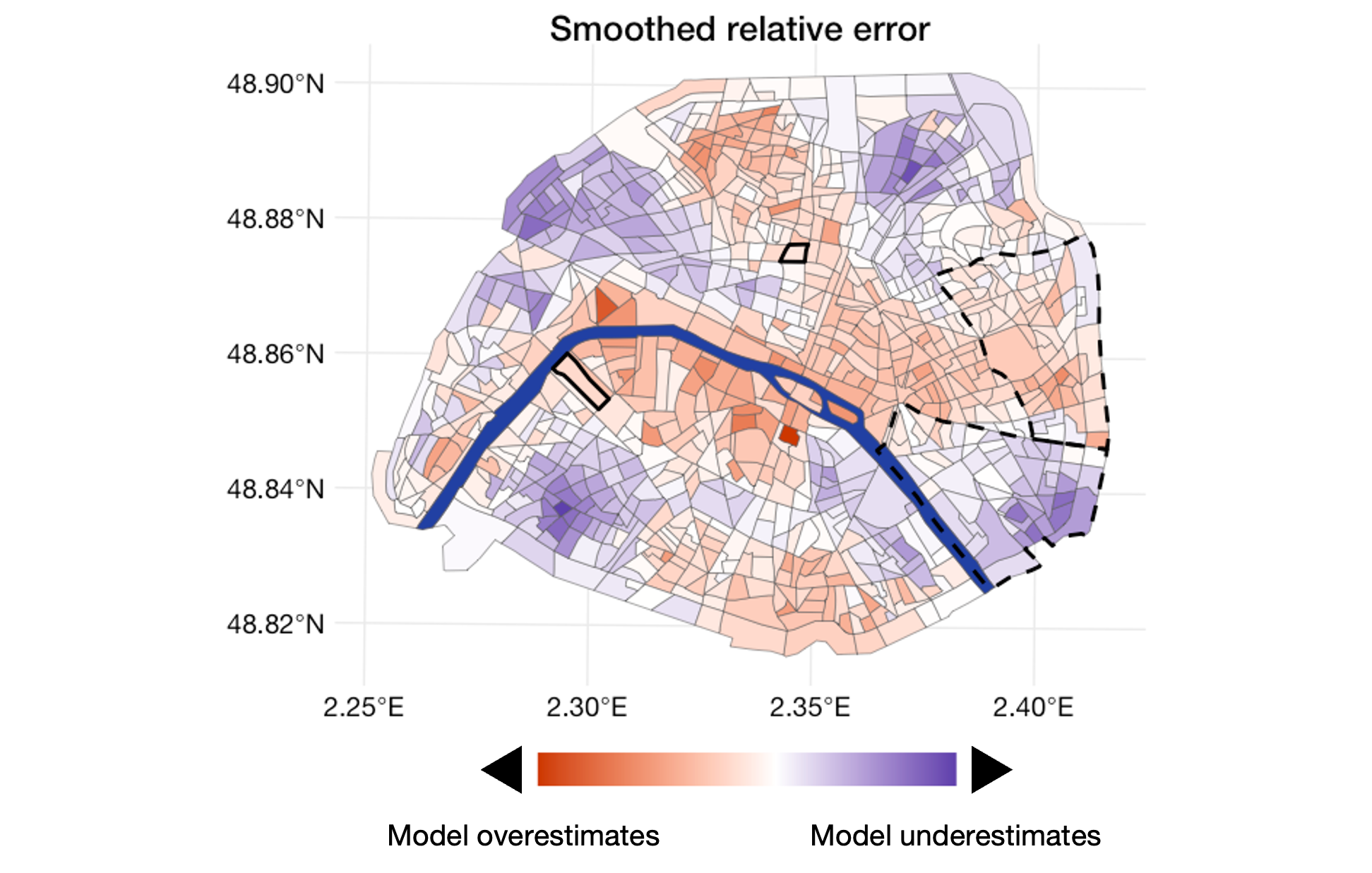
Figure 1: Relative estimation error per $m^{2}$ in different sub-regions. The values are smoothed across spatial neighbors to emphasize the spatial correlation as outlined in Section 3.2.

Finally, as mentioned above, geolocation paired with housing has a long history of undesirable disparities, which makes the use of location in predictive models prone to perpetuating biases. Hence, identifying geospatial biases should be one of the priorities for policymakers. Although the socioeconomic status of neighborhoods can and does change over time, this change is often slow, as documented by rosenthal2015change. For instance, heblich2021east showed that pollution levels from the 1800s could still predict the share of low-skilled workers in a neighborhood, even after the removal of industrial sites responsible for pollution. If such effects can persist in time, using models trained to replicate past events might only reinforce existing disparities.

1.1 Main contributions

Motivated by the aforementioned ethical concerns, including income segregation, and with the objective of deepening our understanding of geospatial disparities, their potential negative impacts, and viable mitigation strategies, we conduct a case study focusing on the Parisian real estate market. Our analysis involves comparing the property estimates provided by a real estate agency with actual observed sale prices. Real estate pricing methodologies are extensively studied and pricing usually depends on a large number of factors, both directly observable and factors that need to be proxied for. At the same time, the real estate market has been extensively studied from the perspective of segregation and other social aspects (chambers_1992_J_Urban_Econ; Kieli_1996_JHE; Myers_2004_J_Urban_Econ; Bayer_2017_J_Urban_Econ). This makes the field an ideal testing ground for the development of algorithms that assess geographical disparities in a more general framework.

Although centered on a specific case study, our approach remains agnostic to the type of predictive models or the variable that is predicted. This broadens the scope of our analysis to include a more general setting. For example, one might examine predictions for the required number of child daycare spots compared to actual application numbers, or similarly, anticipated passenger volume in contrast to the total journeys taken. In each scenario, disparities in calibration and fairness across regions could lead to variations in recommended policy actions.

More specifically to our case study, we are interested in the error rates of the model. The average observed price difference is €203 per square meter (or €1179 in absolute terms) relative to a median sales price of €10,388 per square meter. Although this error is extremely small in a global context, Figure 1 shows that these errors are not necessarily uniformly distributed, suggesting a potential inclination of the predictive model to overestimate sale prices in some neighborhoods and underestimate them in others, even for properties with similar attributes. Given the anchoring effect of an initial valuation, this might lead to undesirable outcomes. Although estimated and realized sale prices are expressed on a continuous scale, we opted for the discretization of values to facilitate the analysis. This approach situates us in an ordinal regression context, enabling the calculation of fairness metrics such as Equalized Odds. The ordinal regression context does not preclude the assessment of the model calibration.

In summary, we find that even if a model is globally well-calibrated, there can be significant differences in fairness metrics in distinct sub-regions. Furthermore, these differences depend on the size and shape of the area under consideration, which pose issues when not all decisions are based on the same aggregation level. To counteract this, we extend previous research on post-processing methods to achieve fairness over a variety of regional groupings. This allows us to change the scores that can be used for policy decisions regardless of the level of analysis. To help researchers in the future, we propose a standard toolbox to measure and mitigate biases based on geospatial datasets.

Specifically, the contributions of the present article can be summarized as follows:

1. We conduct an examination of model errors using post-processing approaches, revealing nuances in predictive biases.

2. We contribute by developing a dedicated framework highlighting geospatial disparities induced by predictive models, aiming to improve algorithmic fairness in geographic contexts and improve the overall understanding of the underlying dynamics.

3. The introduction of a practical case study using Parisian real estate data empowers decision makers to scrutinize disparities in proposals, fostering informed decision-making, and ensuring equitable assessment of geographic considerations.

We begin by providing an overview of the geographic disparity problem and introducing the associated notation in Section 2. Subsequently, in Section 3, we conduct numerical experiments using Parisian real estate data to showcase the intricacies of the issue and to derive associated insights. Within our comprehensive bias mitigation framework, we illustrate, by an example in Section LABEL:sec:detect-and-mitig, how various post-processing techniques can be applied within our contextual framework.

1.2 Related work

Much of this work aligns with the literature on biases and fairness with geographical considerations. The notion of “(geo)spatial bias” resonates with the previously explored notion of “spatial equity” (or “spatial fairness”) in hay1995concepts, which emphasizes the fair distribution of resources and opportunities across various geographical areas. This concern has attracted the attention of researchers from different domains, spanning from public health, where the emphasis lies on ensuring an equitable allocation of medical and health resources to the public (bigman2000spatial; mattei2018fairness), to urban greenery, where endeavors are directed towards developing urban parks that transcend socioeconomic and ethnic boundaries (comber2008using; tan2017effects; yang2020understanding). The goal of understanding (ratz2023fairness; hu2023sequentially) (or mitigating (chzhen2022minimax; hu2023fairness; charpentier2023mitigating)) these biases is to scrutinize biased scores (or transform them into equitable ones). Following a simple privacy-preserving framework, we study spatial disparities with limited information about descriptive features and the learning process of the predictive model. However, we retain data on the geographical location, true score, and model score, as detailed in the real estate case study in Section 3. This justification supports the application of post-processing techniques that can be implemented in addition to any predictive model.

2 Problem statement

In predictive modeling, standard tasks include regression for predicting real-valued outputs and binary classification for categorization into two classes. In the regression task, predicting real values poses challenges for label-conditional modeling or measurement because of the nature of continuous random variables (no mass), which hinders the assessment of the Equalized Odds notion of fairness defined in the next section. To simplify theoretical considerations and enable the comparison of classes within a distribution, one effective approach is to discretize the task into a set of bins while preserving the order of the bins. This practice, often used in decision-making, is known as the ordinal regression case (see gutierrez2015ordinal). Our objective is to predict outcomes within an ordered set $\mathcal{Y}:=[K]=\{1,\ldots,K\}$—also known as a form of multi-class classification (see tewari2007consistency; kolo2011binary). More specifically, we aim to understand how predictors impact different response levels. We denote $\mathcal{X}\subset\mathbb{R}^{d}$ the feature space and we let $\mathcal{H}$ be the set of all predictors of the form $h:\mathcal{X}\to\mathcal{Y}$.

Given our assumption that both the predictive model $h\in\mathcal{H}$ and the data $\boldsymbol{X}\in\mathcal{X}$ are unknown (at least partially), the choice of ordinal regression allows for a more robust approach that is especially effective against skewed distributions with well-positioned cuts for generating bins.

Additionally, we define a sensitive attribute as a characteristic that is considered sensitive because of its potential to introduce bias or discrimination in decision-making processes. This sensitive attribute, denoted $A\in\mathcal{A}$ with $\mathcal{A}:=[M]=\{1,\ldots,M\}$ is herein defined as a discrete group representing specific geographic locations, also known as Geospatial Data. The sensitive attribute $A$ represents a geographical segmentation for which obtaining fair predictions is desirable. This choice of segmentation may be driven by the nature of the data. Certain geographic indicators may be provided based on one partitioning, for example, according to political zone delineations, whereas others may be provided based on a different partitioning, for example, according to administrative delineations. When creating the dataset used for the predictive task, the modeler must make choices to group values on a common spatial scale. Additionally, to comply with data protection and anonymity rules, the values provided on a certain geographical scale may result from a different spatial aggregation from one geographic area to another. When a geographic area lacks a sufficient number of observations, the organization responsible for their dissemination must resort to spatial aggregation to ensure anonymity. Whether the aggregation is due to common scaling or compliance with legal rules, the choices made to define geographic segmentation may not be inherently neutral. This naturally creates a conundrum for any analysis, because the aggregation level of the data can either hide or emphasize certain aspects inherent in the data.

In this context, our aim is to investigate whether a well-calibrated model might exhibit bias based on geolocations. To achieve this, we will introduce metrics designed to assess both model calibration and model unfairness.

Remark 2.1 (The term “fairness”)

In lieu of the term “fairness”, using a more neutral expression such as “unbiased” or equivalent expressions for “unfairness”would be more apt to use in our discussion. The intent behind using (un-)fairness is not to suggest a discriminatory usage of the data per se but rather to emphasize the inequity in under-evaluation. It’s crucial to note that the term “unfairness” is employed here without a negative connotation, as a not fair outcome might be positive for some. The decision of using the term “unfairness” is made to maintain consistency with the established language in the algorithmic fairness literature, where this term is commonly used to denote disparities, despite the absence of an inherently negative implication in our specific context.

Throughout this article, we represent real-valued tasks as $Z$ or $\hat{Z}$ and multi-class tasks as $Y$ or $\hat{Y}$.

2.1 Background on Model Calibration

In traditional regression, a model output denoted as $\hat{Z}$ is considered well-calibrated for $Z$ when (calib2019reg):

$$\mathbb{E}\left[Z\mid\hat{Z}\right]=\hat{Z}\enspace.$$

Let $(\boldsymbol{X},Y)$ be a random tuple with distribution $\mathbb{P}$. In the context of our study, where we focus on ordinal regression denoted as $\mathcal{Y}=[K]$, where $K>0$ is a positive integer, a model $h\in\mathcal{H}$ is deemed well-calibrated in predicting the distribution of confident scores $\hat{\boldsymbol{P}}$ (widmann2019calibration) if:

$$\mathbb{P}(Y=k|\,\hat{\boldsymbol{P}}=\hat{\boldsymbol{p}})=\hat{p}_{k},\quad\text{forall}k\in[K]\enspace,$$

where $\hat{\boldsymbol{p}}=(\hat{p}_{1},\ldots,\hat{p}_{K})$ and $\hat{p}_{k}$ represents the (confidence) score or probability estimate for class $k$ under the model $h$. This calibration concept extends to group-wise calibration when considering a sensitive attribute (widmann2019calibration; wang2020towards). In this scenario, a strongly calibrated model is achieved when:

$$\mathbb{P}(Y=k|\,\hat{\boldsymbol{P}}=\hat{\boldsymbol{p}},\,A=a)=\hat{p}_{k},\quad\text{forall}k\in[K]\text{,andforall}a\in A\enspace.$$

In other words, the model is strongly calibrated if the conditional probability of the true class being $k$ matches the predicted probability for all classes $k$, for all geographical regions $a$. This definition can be undermined to acquire a weakly calibrated model:

$$\mathbb{P}(Y=\arg\max_{k}\hat{P}_{k}\,|\,\max_{k}\hat{P}_{k}=\hat{p}_{k},\,A=a)=\hat{p}_{k},\quad\text{forall}a\in A\enspace.$$

In simpler terms, weak calibration means that the highest predicted probability is used as a threshold and the model is considered calibrated if the true class matches the highest probability.

Furthermore, we introduce the group-wise measure of calibration error, known in the calibration literature as the Expected Calibration Error (ECE) (naeini2015obtaining). We specifically measure group-wise calibration in its weak form, denoted as $\mathcal{U}_{ECE}$, as presented below. Note that, in practical scenarios, the distribution $\mathbb{P}$ is not known. Instead, given empirical data $(\boldsymbol{X}_{i},Y_{i})_{i=1,\ldots,n}$ as $n$ i.i.d. copies of $(\boldsymbol{X},Y)$, we work with the empirical distribution $\hat{\mathbb{P}}_{(\boldsymbol{X}_{i},Y_{i})_{i}}$ (or $\hat{\mathbb{P}}$ for ease of reading), defined as

$$\hat{\mathbb{P}}:=\frac{1}{n}\sum_{i=1}^{n}\delta_{(\boldsymbol{X}_{i},Y_{i})}\enspace.$$

Let the interval $[0,1]$ be partitioned into $B$ bins based on quantiles of $\max_{k}\hat{p}_{k}$ values, where each bin $b\in[B]$ is associated with the set $\mathcal{I}_{b}$ containing the indices of instances within that bin. This partitioning is used in the subsequent definition of the ECE, which is applicable to the multi-class classification framework and thereby extends to ordinal regression.

Definition 2.1 (Model calibration in multi-class classification).

To quantify the ECE, we introduce the accuracy and confidence measures within each bin $b\in[B]$:

$$\text{\textit{(accuracy)}}\ \ \textrm{acc}(\mathcal{I}_{b})=\hat{\mathbb{P}}_{(\boldsymbol{X}_{i},Y_{i})_{i\in\mathcal{I}_{b}}}(Y=\hat{Y})\quad;\quad\text{\textit{(confidence)}}\ \ \textrm{conf}(\mathcal{I}_{b})=\hat{\mathbb{E}}_{(\boldsymbol{X}_{i},Y_{i})_{i\in\mathcal{I}_{b}}}(\max_{k}\hat{p}_{k})\enspace.$$

The calibration error measure for a model $h\in\mathcal{H}$ is then defined as

$$\mathcal{U}_{ECE}(h):=\frac{1}{n}\sum_{b\in[B]}|\mathcal{I}_{b}|\cdot\left|\textrm{acc}(\mathcal{I}_{b})-\textrm{conf}(\mathcal{I}_{b})\right|\enspace,$$

and model $h$ is considered (group-wise) well-calibrated i.f.f. $\mathcal{U}_{ECE}(h)=0$.

The above definition permits the measurement of calibration within a multi-class classification framework, achieved by evaluating the model’s confidence in predicting a specific class against the actual frequency of that class in the observed events. This calibration metric can be calculated within any subregion that includes a sufficient number of datapoints for binning, which is crucial for understanding the far off predictions in a more localized framework. In real estate valuation, where the initial model price acts as an anchor for future decisions, achieving good calibration is therefore essential. Although some error is to be expected, localized variations in error rates may lead to systematic over- or under-valuation in specific areas due to differences in the locally prevalent price category, even if the model is globally well-calibrated. To consider such disparities more specifically, we extend this study beyond calibration alone, with a specific focus on algorithmic fairness and underlying geospatial disparities.

2.2 Background on Algorithmic Fairness

In the present article, we consider two types of fairness evaluation: Demographic Parity (calders2009building) (DP), which asks for independence of the predictive model from the sensitive attribute, and Equalized Odds (EO) (hardt2016equality), which seeks independence conditional on all values of the label space. These definitions, classically considered in binary classification tasks, naturally extend to the multi-class classification framework, as demonstrated in alghamdi2022beyond and denis2021fairness.

2.2.1 Demographic Parity

We let $\hat{Y}$ be the output of the predictive model $h\in\mathcal{H}$ defined on $\mathcal{X}$. From the algorithmic fairness literature, we define the (empirical) unfairness under DP as follows:

Definition 2.2 (Fairness under Demographic Parity).

The unfairness under DP of a classifier $h$ is quantified by

$$\mathcal{U}_{DP}(h):=\max_{a\in\mathcal{A},k\in[K]}\left|\,\hat{\mathbb{P}}(\hat{Y}=k|\textpm\,A=a)-\hat{\mathbb{P}}(\hat{Y}=k)\,\right|\enspace.$$

A model $h$ is called (empirically) exactly fair under DP i.f.f. $\mathcal{U}_{DP}(h)=0$.

Intuitively, DP serves as a widely adopted measure of unfairness that is applicable to various tasks, including regression and classification. This measure holds the advantage of being recognized in legal contexts and regulations. Nevertheless, in situations where the label $Y$ is assumed to be unbiased, there emerges a preference for a more nuanced measure of unfairness. Specifically, DP may hinder the realization of an ideal prediction scenario, such as granting loans precisely to those who are unlikely to default.

2.2.2 Equalized Odds

We assume knowledge of the true and unbiased label $Y$. Another notion of fairness is EO, with its associated unfairness measure defined as follows:

Definition 2.3 (Fairness under Equalized Odds).

The unfairness under EO of a classifier $h$ is quantified by

$$\mathcal{U}_{EO}(h):=\max_{a\in\mathcal{A},k,k^{\prime}\in[K]}\left|\,\hat{\mathbb{P}}(\hat{Y}=k|\,Y\,=k^{\prime},\,A=a)-\hat{\mathbb{P}}(\hat{Y}=k|\,Y=k^{\prime}\,)\right|\enspace.$$

A model $h$ is called (empirically) fair under EO i.f.f. $\mathcal{U}_{EO}(h)=0$.

Ultimately, considering a model $h\in\mathcal{H}$, our objective is to investigate biases related to the model calibration and unfairness defined above, specifically the measures $\left(\mathcal{U}_{ECE}(h),\mathcal{U}_{DP}(h)\right)$ or $\left(\mathcal{U}_{ECE}(h),\mathcal{U}_{EO}(h)\right)$. In the next section, we delve into the case study using Parisian real estate data, where we designate $\hat{Y}$ as the estimated price per $m^{2}$ and $Y$ as the sold price per $m^{2}$.

Remark 1 (Achieving calibration and unfairness).

Achieving group-wise calibration and EO simultaneously has been demonstrated to be impossible, except in highly constrained cases (kleinberg2016inherent; pleiss2017fairness) or by relaxing the EO property to proportional equality, leading to the simultaneous optimization of both fairness and calibration (brahmbhatt2023towards). Similarly, incorporating notions of fairness through calibration is feasible when employing global calibration scores (holtgen2023richness). Despite this, the dependencies between calibration and fairness cannot be generalized, particularly with between-group calibration. Deviations from this measure may reveal unfairness in certain situations but not in others, depending on the specified definition of fairness (loi2022calibration). As a result, calibration and fairness have been studied independently, with fairness primarily assessed through the EO definition, among other factors.

3 Detecting Geographic disparities

We present our main insights through a case study of Parisian real estate, in which we consider different levels of aggregation and highlight how both calibration and fairness-related metrics change across them. Our main goal is to study disparities localized in sub-regions, between predictions made, and labels obtained throughout a test period. In this context, we analyze how model error rates differ across spatial regions, and quantify them using fairness measures. Methods to mitigate some of these biases will be addressed in Section LABEL:sec:detect-and-mitig.

3.1 Data

For our illustrations, we use data obtained from Meilleurs Agents, a French Real Estate platform that produces data on the residential market and operates a free online automatic valuation model (AVM). We have access to both the estimated price of the underlying property and realized net sale price. We consider the realized sale price as the true underlying value $Z$ that we attempt to approximate with the model prediction $\hat{Z}$. Along with the realized and estimated prizes, we also have access to the approximate location and amount of square meters ($m^{2}$) of the property. In total, we obtained approximately 25,700 observations from the Paris Metropolitan Area, of which approximately 11,600 were located in the city of Paris, collected throughout 2019. We use the prices per $m^{2}$ to normalize the errors by property size. Further, we restrict our analysis to observations located within the city of Paris, as there appear to be significant differences in the per $m^{2}$ prices between the core city (Paris intra-muros) and the surrounding areas. See Figure LABEL:fig:plot_price_diff in the appendix for a visual representation. We also removed outliers with a price per square meter of over 20,000€ and observations from mostly commercial areas. In all, we then have access to 11,500 observations after these basic cleaning steps.

Our Data contains geospatial information, aggregated at the IRIS (Ilots Regroupés pour l’Information Statistique) level, a statistical unit defined and published by the French National Institute of Statistics and Economic Studies. Each IRIS region represents a clearly defined area within France and many publicly available economic and societal indicators have been published on this level of granularity. The population within each unit generally consists of between 1,800 and 5,000 inhabitants, which live within a homogeneous living environment, which makes this unit particularly suitable for our analysis. In total, our observations are divided across 878 iris regions.

3.1.1 Defining Neighbors

The city of Paris is divided into 20 administrative units called arrondissements, each grouping between 14 and 96 IRIS regions. It is important to note that an IRIS region cannot belong to multiple arrondissements. Much information about real estate is typically aggregated at this level. However, for our analysis, this unit is too coarse, as there is still considerable heterogeneity within them as can be seen for example in Figure 1. Instead, we opt for a more flexible definition of spatial regions that takes advantage of the homogeneity within each IRIS region. As the size of the area of each IRIS differs considerably, simply defining higher levels by Euclidean distance from a given point might pose problems, as it could include many dense but heterogeneous regions on one end of the spectrum or only a few on the other. To take advantage of the differing sizes and homogeneity within the IRIS regions, we define a neighborhood graph. In its general form, a graph is an ordered pair $\mathcal{G}=(\mathcal{V},\mathcal{E})$ of vertices and edges. In our application, each vertex represents an IRIS region, and each edge represents a neighboring relation. Here, a neighboring relation is defined as the presence of an intersection between two polygons, including their boundaries, defining an IRIS region. That is, edge $(i,j)$ is present in edge set $\mathcal{E}$ if the polygons of regions $i$ and $j$ intersect. The graph can then be represented as an $n\times n$ matrix $V$, called the adjacency matrix, where $V_{i,j}\in\{0,1\}$ with $V_{i,j}=1$ if $(i,j)\in\mathcal{E}$. That is, each entry in the adjacency matrix is equal to $1$ if two vertices are in a neighborhood relationship with each other. Representing neighborhood relations using an adjacency matrix has the advantage that non-intermediate connections can be easily obtained by successively multiplying the adjacency matrix by itself. That is, all nonzero elements of $V^{2}$ represent neighborhoods that are either immediately adjacent to a given region (the direct neighbors) or are adjacent to the direct neighbors (the neighbors of the direct neighbors). This process can be repeated $n$ times to obtain neighbors that can be reached within an $n$ length path. This provides a more natural way to define neighborhoods, as with each increasing path length, an entire homogeneous region is added to the higher-level aggregation. Figure 2 illustrates how the neighborhood set for a particular IRIS community can be calculated.

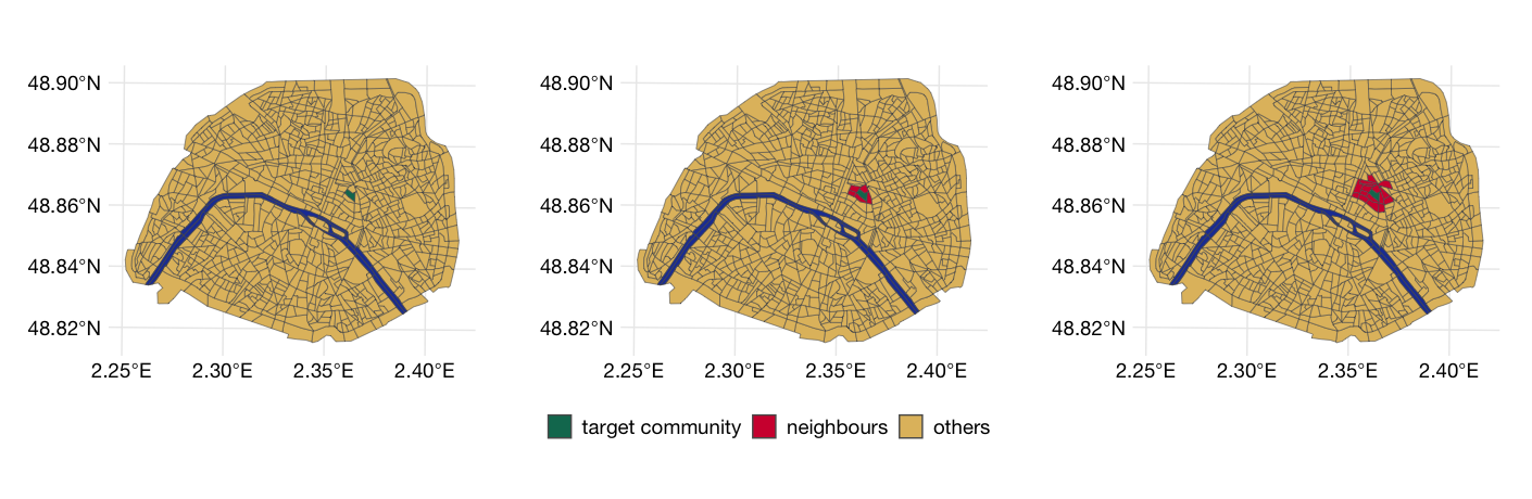
Figure 2: A sampled IRIS region within Paris (left pane) and its immediate adjacent neighbors (center pane) and the second level neighbors (right pane). The Seine River is depicted in blue whereas all other regions are depicted in yellow.

3.2 Neighborhood-Based Smoothing

To reveal spatial structures, as shown in Figure 1, the raw data must be processed and filtered. One reason for this is that the observations are not uniformly distributed across IRIS regions. This naturally leads to different levels of confidence when summary statistics for each IRIS, such as the mean relative model error per $m^{2}$, are considered. The core idea of spatial smoothing is to use an average over a larger area, which should provide a more robust estimate. Applying a (weighted) mean function has the effect of a low-pass filter, which removes sharp edges between the IRIS regions, and hence produces an output that has a more pronounced spatial correlation, revealing the underlying structure. Kernel based methods are common within spatial analysis (see, e.g., genebes2018spatial). However, as discussed above, in our case, the data is already aggregated at the IRIS level, which restricts the application of spatial kernel-based smoothing whose bandwidth operates on Euclidean distances.

As an alternative, we use the constructed neighborhood graph and the path length between regions as the argument of a weight function, similar to kernel-based methods. That is, for a given variable observed at IRIS level $x$, the smoothed value for region $r_{i}$, denoted as $\lambda_{\omega}(x_{i})$ can be written as:

$$\lambda_{\omega}(x_{i})=\frac{1}{\sum_{j=1}^{n}{\omega}(r_{i},r_{j})}\sum_{j=1}^{n}{\omega}(r_{i},r_{j})x_{i}\enspace.$$ (1)

For example, let $d(r_{i},r_{j})$ be the path length between regions $r_{i}$ and $r_{j}$, then a simple way to define $\omega(r_{i},r_{j})$ is: