Exploring one giga electronvolt cosmic gamma rays with a Cherenkov plenoscope capable of recording atmospheric light fields
Part 1: Optics

Abstract

Detecting cosmic gamma rays at high rates is the key to time-resolve the acceleration of particles within some of the most powerful events in the universe. Time-resolving the emission of gamma rays from merging celestial bodies, apparently random bursts of gamma rays, recurring novas in binary systems, flaring jets from active galactic nuclei, clocking pulsars, and many more became a critical contribution to astronomy. For good timing on account of high rates, we would ideally collect the naturally more abundant, low energetic gamma rays in the domain of one giga electronvolt in large areas. Satellites detect low energetic gamma rays but only in small collecting areas. Cherenkov telescopes have large collecting areas but can only detect the rare, high energetic gamma rays. To detect gamma rays with lower energies, Cherenkov-telescopes need to increase in precision and size. But when we push the concept of the –far/tele– seeing Cherenkov telescope accordingly, the telescope’s physical limits show more clearly. The narrower depth-of-field of larger mirrors, the aberrations of mirrors, and the deformations of mirrors and mechanics all blur the telescope’s image. To overcome these limits, we propose to record the –full/plenum– Cherenkov-light field of an atmospheric shower, i.e. recording the directions and impacts of each individual Cherenkov photon simultaneously, with a novel class of instrument. This novel Cherenkov plenoscope can turn a narrow depth-of-field into the perception of depth, can compensate aberrations, and can tolerate deformations. We design a Cherenkov plenoscope to explore timing by detecting low energetic gamma rays in large areas.

16cm(2.75cm,26.65cm) Astroparticle Pysics’s internal reference: 102933, volume: 158
International Standard Serial Number (ISSN): 0927-6505
Digital Object Identifier (DOI): https://doi.org/10.1016/j.astropartphys.2024.102933 [mpik] organization=Max-Planck-Institute for Nuclear Physics, addressline=Saupfercheckweg 1, city=Heidelberg, postcode=69117, state=Germany [ethz_ipa] organization=Institute for Particle Physics and Astrophysics, ETH-Zurich, addressline=Otto-Stern-Weg 5, city=Zurich, postcode=8093, state=Switzerland [ethz_geo] organization=Dept. of Civil, Environmental and Geomatic Engineering, ETH-Zurich, addressline=Stefano-Franscini-Platz 5, city=Zurich, postcode=8093, state=Switzerland

1 Introduction

The observation of cosmic gamma rays offers unique insights to the most violent and energetic events in the universe. Unlike the lower energetic light ranging from radio to X-rays, which mostly originates in thermal emission of cosmic remnants slowly transitioning towards a new equilibrium, the higher energetic gamma rays are often a direct probe of sudden cosmic events. In many cosmic sources, we observe flares and bursts of gamma rays. Because of this, the observation and interpretation of timing in the sky of gamma rays became a vivid part of astronomy. Already with our current instruments, we observe occasional and apparently random bursts (Ackermann et al., 2014) of gamma rays so bright that they outshine an entire galaxy. We observe rapid changes in the flux of gamma rays coming from active galactic nuclei which host massive black holes. Each change in flux is a probe to better constrain the inner processes in the vicinity of the black hole, complementary to and often better than probes based on angular resolution (Aleksić et al., 2014). Pulsars, which were expected to have steady pulsed emissions, apparently also can emit powerful bursts of gamma rays (Tavani et al., 2011). With the observations of gravitational waves from cosmic mergers, astronomy starts to look for counterparts in gamma rays (Abbott et al., 2017) hoping that the variations in time of both gravitational waves and gamma rays will allow to better understand the moments before, and during these cosmic catastrophes.

However, the frequent use of timing in the astronomy of gamma rays pushed our current instruments to their limits. Cosmic sources emit gamma rays mostly with the energy distributed in steep power laws where lower energetic gamma rays in the 1 GeV domain are much more abundant than higher energetic gamma rays with 10 GeV or above. Pulsars even have their emission cut off above $\sim 10\,$GeV (Ailu et al., 2008, Abdo et al., 2009). Also the universe is not transparent for higher energetic gamma rays which are absorbed by the infrared light found in between galaxies (Albert et al., 2008). To improve the exploration of timing, for not only nearby but also for distant sources, we want to detect many low energetic gamma rays in large collecting areas in order to gather significant statistics in short time.

Motivated by initial findings (Mueller, 2019), we propose to combine the atmospheric Cherenkov technique with plenoptics to build the Cherenkov plenoscope, a novel class of instrument, which can detect gamma rays with energies down to $\approx 1\,$GeV in large collecting areas exceeding $\approx 10^{3}\,$m². We present a specific Cherenkov plenoscope, named Portal, which can be built with existing technology and which might become the next generation’s explorer for the timing in the sky of gamma rays.

1.1 Current Methods

Currently, gamma rays in the $1\,$GeV domain are only accessible with detectors in space like Fermi-LAT (Acero et al., 2015) or AGILE (Tavani et al., 2011). Detectors in space directly interact with the cosmic particle and have typically a tracker to measure the direction, a calorimeter to measure the energy, and a surrounding detector for electrically charged cosmic rays to distinguish them from neutral gamma rays. Despite their high cost, detectors in space provide only a modest $\sim 1\,$m² area to detect gamma rays. For steady sources, the small area can be compensated by multi-year exposure (Acero et al., 2015), but it significantly limits the exploration of the highly-variable sky of gamma rays with energies in the GeV domain.

As the collecting area of detectors in space is not expected to rapidly grow in the foreseeable future, we want to shift our focus to indirect detection in earth’s atmosphere using Cherenkov light. Here cosmic particles induce showers in earth’s atmosphere. Only a few products from the shower reach the ground, for example a flash of Cherenkov photons. The Cherenkov telescope’s mirror and image camera effectively bin the photons into a sequence of images. A trigger searches this sequence of images for flashes of Cherenkov photons and redirects those images to permanent storage while it dismisses the rest. The trigger is a critical, but necessary compromise that reduces the extensive and continuous response from the photosensors down to an amount that one can process and store. The sequences of images selected by the trigger are then the basis (Hillas, 1985) to reconstruct the cosmic particle’s energy, direction, and type. The effective collecting area of a Cherenkov telescope to detect a gamma ray can be as large as the area illuminated by the gamma ray’s shower on ground, reaching $\sim 10^{5}\,$m². The fact that a Cherenkov telescope effectively detects gamma rays in an area much larger than its own physical size makes it very efficient. Current (Ailu et al., 2008) and upcoming (Bernlöhr et al., 2013) Cherenkov telescopes can detect gamma rays with energies as low as 20 GeV. The lowest detectable energy is governed by the area and efficiency to detect Cherenkov photons, as their number is roughly proportional to the cosmic particle’s energy (de Naurois and Mazin, 2015), and experience shows that a minimum of $\approx$100 photons has to be detected in order to reconstruct a cosmic particle from its shower’s Cherenkov light. Cherenkov telescopes have put great effort into lowering their energetic thresholds, by enlarging their mirrors, by using more efficient photosensors, by improving the reconstruction, and identification of showers, and by moving onto mountains, closer to the shower, where the density of Cherenkov photons is higher. For a proposed array of five 20 m large Cherenkov telescopes at 5 km altitude, a threshold of 5 GeV was targeted (Aharonian et al., 2001).

However, two physical limits reduce the maximum diameter for a mirror in a Cherenkov telescope to $\sim 30\,$m. First, the narrower depth-of-field on larger mirrors blurs more parts of the shower’s image and thus erodes the power to reconstruct the cosmic particle (Hofmann, 2001, Mirzoyan et al., 1996). Showers do not happen in a field far away but have their maximum usually in a depth not further than 30 km in front of the mirror while they naturally extend over a depth in the range of 10 km. The narrow depth-of-field is a central reason why the mirrors in the next generation of Cherenkov telescopes will not exceed $\sim 23\,$m in diameter (Bernlöhr et al., 2013). Second, the square-cube-law complicates the construction of larger Cherenkov telescopes rapidly. When enlarging a telescope, the forces scale cubic with the dimensions but the areas, which have to tolerate these forces, only scale quadratic. This limits the cost effective construction of a large Cherenkov telescope with sufficient rigidity for the optics.

Since large telescopes have their limits, one could also consider to solve the technological challenge of combining the images from many small telescopes. The idea (Jung et al., 2005) is to lower the energetic threshold by building an array of small telescopes which feed their continuous sequences of images into a central trigger. The critical challenge is that all signals need to be transmitted to a central location, where they are appropriately delayed according to the telescopes pointing, and summed up into pixels of an image. However, only in the image seen by the central trigger the Cherenkov light emerges out of the random light coming from the nightly sky. Thus the individual telescopes can not reduce their signals before they send them to the central trigger. Overall, the required rates of data that need to be transmitted over the array’s size, delayed, and reorganized into an image, be it analog or digital, are daunting. Although impressive progress (Schroedter et al., 2009, López-Coto et al., 2016, Dickinson et al., 2018) was made, today the central trigger for an array of telescopes remains a challenge. Today, the first trigger, where most information is reduced, is bound to the individual telescope (Bulian et al., 1998, Funk et al., 2004, Weinstein et al., 2007, López-Coto et al., 2016).

1.2 Proposing a Novel Class of Atmospheric Cherenkov Instrument

When one investigates the causes for the telescope’s narrow depth-of-field, and its suffering from deformations and aberrations it turns out that all this is related to the telescope not knowing the position where a photon is reflected on its mirror.

Assume there was a novel class of instrument just like the telescope but with a different camera. Instead of only measuring the position where a photon is absorbed on the camera’s screen, the novel camera was further able to measure the direction of the photon relative to its screen. Given the alignment of the camera relative to the mirror, one can compute the trajectory of the photon on its path from the mirror towards the camera. Given further the shape of the mirror, one can compute the photon’s trajectory before it gets reflected by the mirror. Given further the pointing of the mirror, one can compute the photon’s trajectory in the atmosphere. Even if the novel instrument’s mirror deformed and its alignment relative to the camera changed, one can still reconstruct the photon’s trajectory correctly as long as one measures the instrument’s alignment and shape.

At this point, when the instrument is capable of reconstructing the trajectories of individual photons, one says: the instrument has plenoptic perception (Lippmann, 1908), and is capable of recording light fields.

From here on, one can mentally leave the instrument’s optics behind and instead concentrate on the recorded trajectories of the photons. Now one can take the observed bundle of photons and simulate the image it would make when one guides it into the perfect model for a telescope with its focus set to an arbitrary depth of one’s choice (Ng et al., 2005). One could make a whole stack of images with the depth set to different foci highlighting different slices of the shower as it progresses downwards in the atmosphere. One could simulate the images that the bundle of photons would make when one guides it into an array of telescopes. Here one could make images seen from different perspectives and apply the established reconstructions used in arrays of Cherenkov telescopes. Of course the images created by a perfect model for a telescope are free of aberrations and distortions (Hanrahan and Ng, 2006). One could also take the bundle of photons and their trajectories to reconstruct the three-dimensional shower in the atmosphere using tomography (Levoy et al., 2006, Arbet Engels, 2017). The only remaining limitations would come from the finite resolution of the camera to measure the photon’s position and direction, and the instrument’s uncertainties about its alignment and shape. Clearly, the possibilities of such an instrument would be remarkable. We call this novel class of instrument the Cherenkov plenoscope.

2 Cherenkov Plenoscope

Both the Cherenkov telescope and -plenoscope use an imaging mirror. But the Cherenkov plenoscope’s camera is different and changes the optics fundamentally.

2.1 Optics

Fig. 1 shows the optics of a telescope and a plenoscope that use identical mirrors. To illustrate the difference in optics, we show on each tele- and plenoscope a single beam, defined as the set of all the optical paths a photon can take to reach a given photosensor. The plenoscope’s camera needs to measure both the position and the direction of the same photon. Measuring the photon’s position on the camera gives the photon’s direction relative to the mirror, and measuring the photon’s direction relative to the camera gives the photon’s position of reflection on the mirror. To achieve this, consider an imaging lens that guides light into a closed box where a plane of photosensors opposes the lens on the back of the box, see Fig. 2. For short, one might call this arrangement an eye. Such an eye can measure the direction of a photon while it can further determine the same photon’s position to have been within the limits of its lens. However, a single eye is not yet enough. For the plenoscope’s camera to not only measure the photon’s direction but also it’s position, one packs multiple, small eyes into a dense array. This array of eyes is called a light-field camera. When one knows the eye in which a photon was absorbed, one has measured the photon’s position on the light-field camera. And when one knows the specific photosensor inside the eye that has absorbed the photon, one has measured the photon’s direction relative to the light-field camera. A light-field camera can measure the trajectories of all photons without blocking and masking them. While the telescope’s beams spread across the entire mirror, the plenoscope’s beams only cover parts of the mirror.

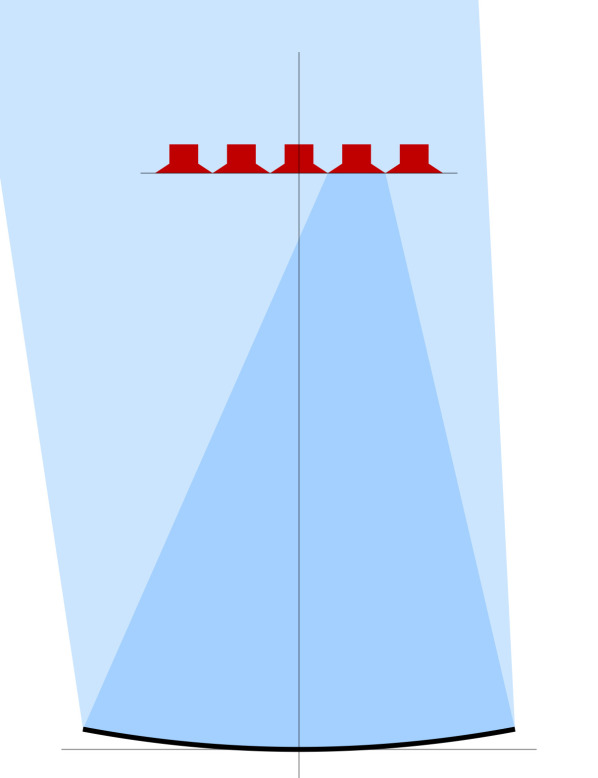
(mirror: good, camera: good)

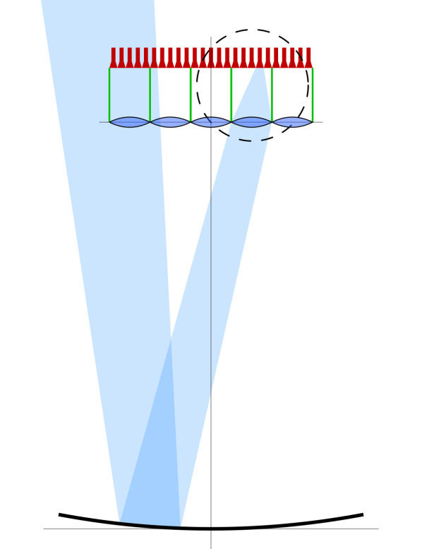
(mirror: good, camera: good)

Figure 1: A telescope on the left and a plenoscope on the right. Both have identical mirrors. photosensors are red. Beams, which bundle all the photons trajectories reaching a given photosensor, are blue. On each instrument only one beam is shown. Fig. 2 shows the dashed circle up close.

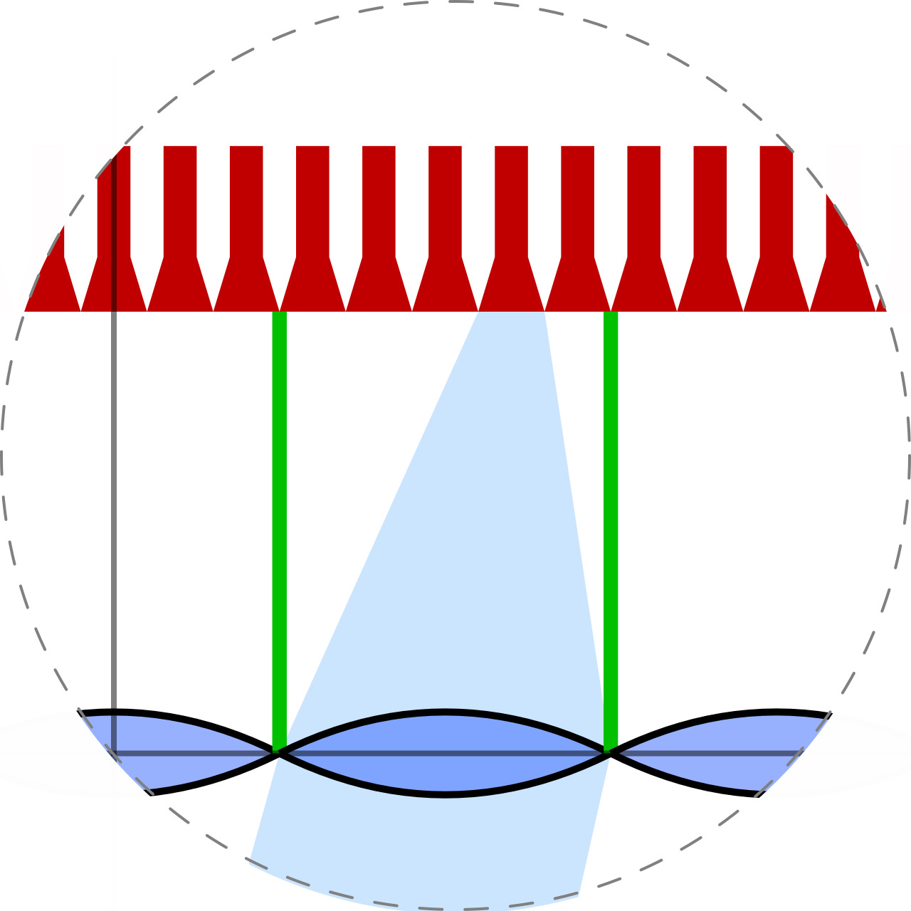
Figure 2: A close-up on the plenoscope’s light-field camera shown in Fig. 1. Green walls are the housings of eyes. Curved black lines show the bi-convex lenses of eyes.

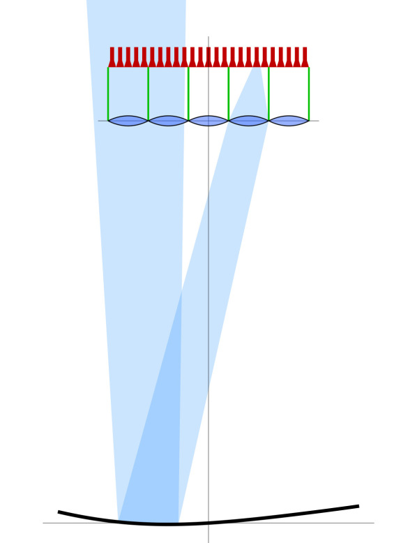
(mirror: deformed, camera: good)

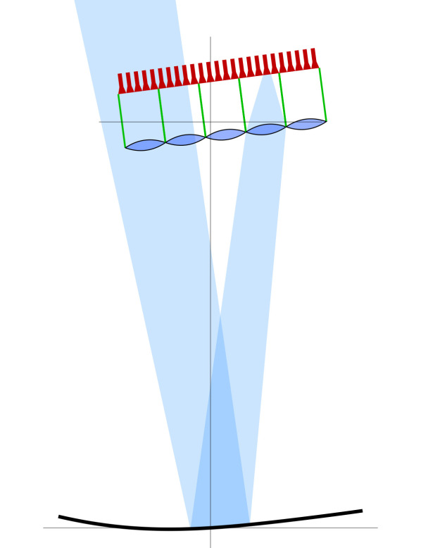
(mirror: deformed, camera: misaligned)

Figure 3: A plenoscope with a deformed mirror on the left and a plenoscope with both a deformed mirror and a misalignment on the right. Compare with the plenoscope’s default geometry in Fig. 1.

Both the telescope and plenoscope shown in Fig. 1 have five directional bins to measure a photon’s direction. The telescope has five photosensors which serve as its directional bins, and the plenoscope has five eyes which serve as its directional bins. While the telescope has only a single positional bin to measure a photon’s point of reflection on its mirror, the plenoscope has five positional bins. In Fig. 2 one finds five photosensors inside each eye of the light-field camera which serve as the plenoscope’s five positional bins.

To convert the telescope’s image camera into the plenoscope’s light-field camera, one has to replace each of the image camera’s photosensors with an eye. The other way around, if one adds the photosensors signals from within each eye into a single signal, the light-field camera degenerates into an image camera. Only if one records the individual signals, one can take advantage of the plenoscope’s individual beams being only effected by small parts of the mirror. This can resolve aberrations.

Aberrations occur when the photon’s position on the camera’s screen not only depends on the photon’s direction relative to the mirror, but also on the photon’s position of reflection on the mirror. So if one can measure the photon’s position of reflection on the mirror, one can compensate aberrations. Fig. 3 shows that the geometry of the plenoscope’s beams change when its mirror is deformed, or its camera is misaligned. However, we will show that this change of the beams geometry does hardly effect the plenoscope’s performance as long as one knows the geometry of the beams. The plenoscope’s ability to compensate deformations is in stark contrast to the telescopes demand for rigidity. Postponing the square-cube-law by compensating deformations is one key in the plenoscope’s quest to be large enough to detect gamma rays with lower energies. But while one could postpone the square-cube-law also on larger telescopes by spending exponentially more resources and engineering, the telescope’s physical limit of a narrowing depth-of-field remains.

2.2 Depth-of-Field

The bigger the mirror of a telescope becomes, the narrower becomes its depth-of-field. The telescope’s depth-of-field is the ‘field’ (range) along its depth (optical axis) where objects create sharp images. When this depth narrows we are forced to adjust the telescope’s focus (Trichard et al., 2015) in order to have at least a sharp image of the most relevant depth while we have to accept blurring in all remaining depth. The thin-lens equation

$$\frac{1}{f} = \frac{1}{g}+\frac{1}{b}$$ (1)

and Fig. 4 describe this blurring and show

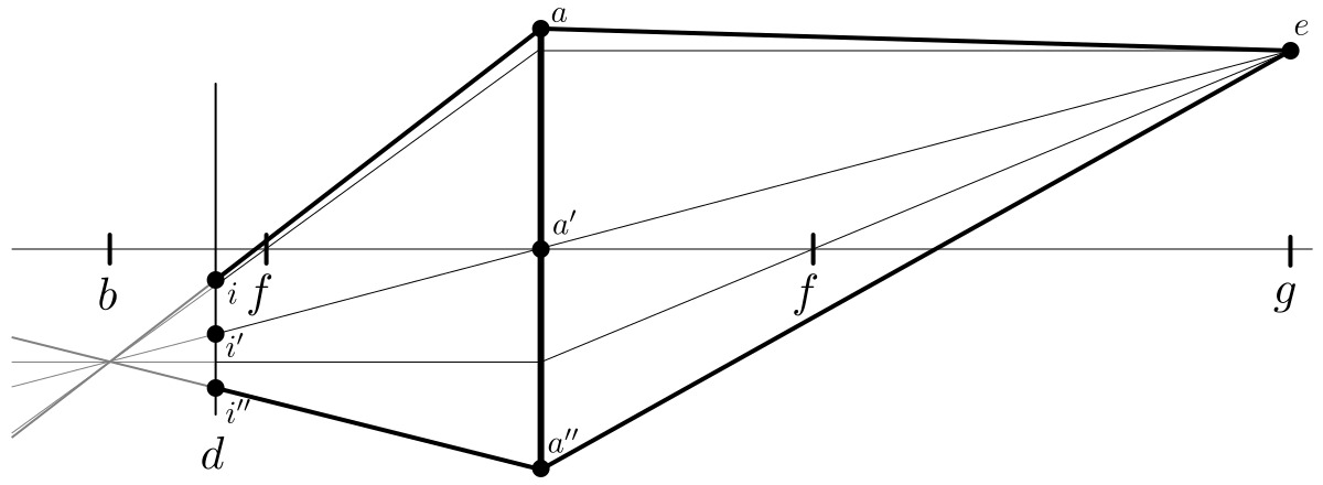
Figure 4: The ‘thin lens’ with focal-length $f$ and aperture $\overline{aa^{\prime\prime}}$. Horizontal line is the optical axis, thick vertical line is the aperture’s principal plane. The three principal rays emitted by an object in depth $g$ converge in the image’s distance $b$. However, the principal rays do not converge on the camera’s screen which is in distance $d\neq b$. The image of the object is not sharp but stretches from $i$ to $i^{\prime\prime}$. For readability, this figure shows a transmitting lens. But Eq. 1 is also valid when the figure was folded along the aperture’s principal plane so that the two focal-points $f$ became one and $g$ and $b$ were on the same site of the aperture. In that case the figure would show a reflective mirror as we find it on most Cherenkov telescopes. In the context of atmospheric Cherenkov emission: note that one can interpret the point $e$ as the location of a nearby charged particle emitting Cherenkov light in a cone along e.g. the lines $\overline{ea}$ and $\overline{ea^{\prime}}$.

the distance $b$ where the image forms and where the camera’s screen must be positioned in order to record a sharp image of an object in depth $g$ when the focal-length is $f$. Fig. 4 shows that the image $i,i^{\prime},i^{\prime\prime}$ is a scaled projection of the aperture $a,a^{\prime},a^{\prime\prime}$. This projection is the reason for the blurring and is referred to as Bokeh in some literature (Merklinger, 1997, Ahnen et al., 2016a).

In Bernlöhr et al. (2013), one finds an estimate

$$g_{\pm} = g(1\pm pg/(2fD))$$ (2)

for the object’s starting depth $g_{-}$ and ending depth $g_{+}$ in order to define the depth-of-field on a Cherenkov telescope. Here $D$ is the diameter of the mirror, and $p$ is the diameter of an area in the camera’s screen from where the light will be further guided into a photosensor. This estimate is based on Hofmann (2001), which also uses Eq. 1. For example, a Cherenkov telescope with $D=71\,$m and $f=106.5\,$m would have a depth-of-field extending from $g_{-}=9.2\,$km to $g_{+}=10.8\,$km when its focus is set to $g=10.0\,$km. This will blur large parts of a shower’s image because a shower’s depth exceeds this only $1.6\,$km narrow depth-of-field by about an order-of-magnitude. In the past, Cherenkov telescopes lowered their energetic threshold by enlarging their mirrors (enlarging $D$ and $f$), by moving up in altitude closer to the shower (lowering $g$), and by increasing angular resolution and the number of photosensors (lowering $p$). But Eq. 2 shows that these three measures all narrow the depth-of-field. Thus imaging itself becomes a physical limit that prevents Cherenkov telescopes from being large enough to observe gamma rays with energies below $\approx 20\,$GeV.

But if the camera in Fig. 4 is a light-field camera, it not only observes that three photons arrive in the points $i$, $i^{\prime}$, and $i^{\prime\prime}$, but it observes that the photons travel on the trajectories $\overline{ia}$, $\overline{i^{\prime}a^{\prime}}$, and $\overline{i^{\prime\prime}a^{\prime\prime}}$. With this one knows that the photons approached on the trajectories $\overline{ae}$, $\overline{a^{\prime}e}$, and $\overline{a^{\prime\prime}e}$. With a light-field camera, one obtains a strong hint that the photons were produced in point $e$ in depth $g$ despite the camera being out of focus with $d\neq b$. On a Cherenkov plenoscope, the narrowness of the depth-of-field expressed in Eq. 2 becomes an estimate for the plenoscope’s resolution of this depth. So the enlarging of the mirror, the increasing of angular resolution, the moving up in altitude onto mountains, all these measures to lower the Cherenkov method’s energetic threshold do not narrow, but actually extend and sharpen the Cherenkov plenoscope’s perception of depth. Therefore, at least from the optic’s point-of-view, the Cherenkov plenoscope is promising to be made large enough in order to detect low energetic gamma rays.

3 Reconstruction and Interpretation

To reconstruct the Cherenkov photons of an atmospheric shower with a Cherenkov plenoscope, while accounting for misalignments and deformations, we propose to describe the perception of the Cherenkov plenoscope with the help of three-dimensional rays. Reconstructing a photon here means to measure its three-dimensional trajectory and its time of arrival.

3.1 Defining the Light-Field Calibration

We describe the perception of an atmospheric Cherenkov instrument using the beams of light that the instrument’s photosensors observe in the atmosphere. We describe a photosensor’s beam using the many optical paths that a photon can travel in order to reach this photosensor. Each of these optical paths is a set

$$\mathcal{P}{} = \begin{Bmatrix}{s_{x}},{s_{y}},{c_{x}},{c_{y}},\tau,\eta\end{Bmatrix}$$ (3)

which describes a ray

$$\vec{r}(\chi) = \underbrace{\begin{pmatrix}s_{x}\\ s_{y}\\ 0\end{pmatrix}}_{\vec{s}}+\chi\underbrace{\begin{pmatrix}c_{x}\\ c_{y}\\ \sqrt{1-{c_{x}}^{2}-{c_{y}}^{2}}\end{pmatrix}}_{\vec{c}}$$ (4)

that the photon travels on, in opposing direction, in order to reach the instrument’s aperture, and later a photosensor. In the same frame, the aperture’s principal plane is the $xy$-plane, and the aperture’s optical axis is the $z$-axis. This way, the ray’s support $\vec{s}$ is within the aperture’s principal plane, and the ray’s direction $\vec{c}$ is pointing from the aperture up into the sky, anti parallel to the incoming Cherenkov photon from a shower. By defining the rays relative to the aperture’s principal plane, the four-tuple ($s_{x}$, $s_{y}$, $c_{x}$, $c_{y}$), compiled from the $xy$-components of the ray’s support $\vec{s}$ and direction $\vec{c}$, is sufficient to describe the geometry of an optical path $\mathcal{P}{}$. Fig. 6 shows a ray $\vec{r}(\chi)$ and its vectors $\vec{s}$ and $\vec{c}$ in a later use to construct image rays.

Because Cherenkov instruments can measure the arriving time of photons in a regime of 1 ns while having optics with sizes in the regime of several $1$ m, one also adds for each path the time $\tau$ that it takes a photon to travel from the aperture’s principal plane to the photosensor. Further, we add relative efficiencies $\eta$ for each path to respect differences in the instrument’s reflection, and transmission. With this, we approximate a photosensor’s beam by using a list of $P$ optical paths

$$\mathcal{B}{} = \begin{bmatrix}\mathcal{P}{}_{1},\mathcal{P}{}_{2},\dots\mathcal{P}{}_{P}\end{bmatrix}.$$ (5)

The optical paths are randomly drawn from a uniform distribution and the number $P$ of paths which reach the given photosensor is sufficiently large to represent the beam appropriately. Now we can describe the perception of an atmospheric Cherenkov instrument with the list

$$\mathcal{G}{} = \begin{bmatrix}\mathcal{B}{}_{1},\mathcal{B}{}_{2},\,\dots\,\mathcal{B}{}_{K}\end{bmatrix}$$ (6)

of its $K$ beams, one beam for each photosensor. We name $\mathcal{G}{}$ the instrument’s light-field calibration.

3.2 Defining the Instrument’s Response

A photosensor measures the arriving time $t^{\prime}$ of a photon. photosensors have limitations, but one can express their response using a list

$$\mathcal{T}{} = [t^{\prime}_{1},\,t^{\prime}_{2},\,\,\dots\,\,t^{\prime}_{L}]$$ (7)

of arriving times of $L$ photons that is most probable to have caused the photosensor’s recorded signal. In turn one can describe the instrument’s total response using a list of lists

$$\mathcal{R}{}_{\text{l}}{} = \begin{bmatrix}\mathcal{T}{}_{1},\mathcal{T}{}_{2},\dots\mathcal{T}{}_{K}\end{bmatrix}$$ (8)

of all the $K$ photosensors responses. Alternatively and equally valid, one can represent this as a histogram with the number of photons $i_{k},t$ in the $k$-th beam and the $t$-slice in time

$$\mathcal{R}{}_{\text{h}}{} = \begin{bmatrix}i_{1,\,1}&i_{1,\,2}&\ldots&i_{1,\,T}\\ i_{2,\,1}&i_{2,\,2}&\ldots&i_{2\,T}\\ \vdots&\vdots&\ddots&\vdots\\ i_{K,\,1}&i_{K,\,2}&\ldots&i_{K,\,T}\\ \end{bmatrix}.$$ (9)

3.3 Reconstructing the Photons Observables

When a photosensor $k$ detects a photon to be absorbed at time $t^{\prime}$ one can use an optical path from within beam $\mathcal{B}{}_{k}$ to compute the time

$$t_{\text{aperture}} = t^{\prime}-\tau_{k}$$ (10)

at when the photon would have passed the aperture’s principal plane. For any moment in time $t$, one can now compute the distance

$$\chi(t) = -\frac{{c_{0}}}{n}(t-t_{\text{aperture}})$$ (11)

that the photon still has to travel before it will reach the aperture’s principal plane. Here $c_{0}$ is the speed of light and $n$ is the refractive index of the instrument’s surrounding medium. With this one can compute the photon’s position $\vec{r}(\chi(t))$ for any moment in time $t$, while keeping in mind that from a single photon’s observables $(x,y,c_{x},c_{y},t^{\prime})$ we can not constrain the time of its creation. Fig. 5 shows the concepts we defined so far. In pale blue one sees some of the photosensors beams $\mathcal{B}{}_{1}$ to $\mathcal{B}{}_{4}$ reaching up from the aperture’s principal plane into the atmosphere. But unlike Fig. 1, this does not show the beams inside the plenoscope which reach from the mirror to the photosensors. In the most left beam $\mathcal{B}{}_{1}$ one can see the rays $\vec{r}(\chi)$ of the optical paths which describe this beam. All the figure shows the same moment in time $t$. Along the beams, darker blue clouds indicate the reconstructed volumes of photons. The darker the blue, the more photons are reconstructed to be in this volume. The volume’s spread depends both on how fuzzy the beam is and on how well the beam’s photosensor can reconstruct the photon’s time of absorption $t^{\prime}$.

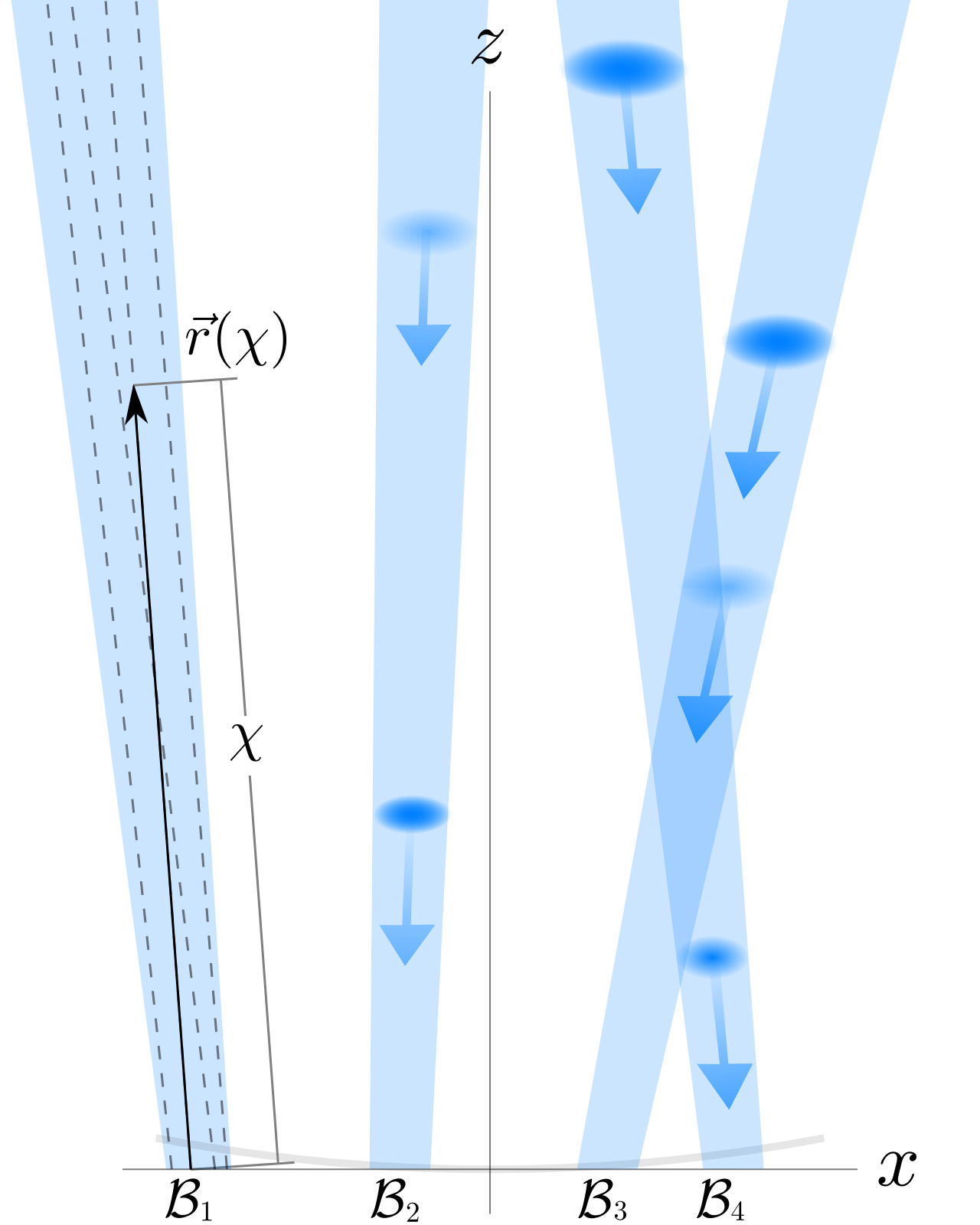
Figure 5: Reconstructing photons on a Cherenkov plenoscope using beams. The plenoscope’s physical mirror is a curve in faint gray. See description on reconstruction in Sec. 3.3. Note that the blue beams $\mathcal{B}{}$ and dashed rays $\vec{r}(\chi)$ start on the aperture’s principal plane ($\vec{r}(\chi=0)$), pass through the physical mirror, and extent up into the sky. On the other hand, the blue-cloudy photons, which represent the physical Cherenkov photons coming down from an atmospheric shower, will not pass the physical mirror. These photons will be reflected on the physical mirror. The light-field calibration does not know on what paths the physical photons find their ways into their photosensors. The light-field calibration does not need to know this. All that the light-field calibration needs to knows is, that a physical photon, which approaches the aperture’s principal plane on a specific ray $\vec{r}_{k}$ (that is a ray within $\mathcal{B}{}_{k}$), will be absorbed by a specific and corresponding photosensor $k$.

When one applies the light-field calibration $\mathcal{G}{}$ to the photosensors responses $\mathcal{R}{}$, the result is a measurement of five observables ($x\,,y\,,c_{x},\,c_{y}\,,t$) for each photon. One might call this measurement a sequence (in time $t$) of light fields ($x\,,y\,,c_{x},\,c_{y}$). There are many interchangeable ways to represent sequences of light fields. For example, in combination with the light-field calibration $\mathcal{G}{}$, the histogram in Eq. 9 or the list of lists in Eq. 8 are possible representations.

4 Imaging

Since Hillas (1985), imaging is well established in the atmospheric Cherenkov method to reconstruct cosmic gamma rays. So projecting the Cherenkov plenoscope’s light field onto an image is a good start to get familiar with plenoptic perception. The idea is to take the Cherenkov plenoscope’s reconstructed photons, defined in Sec. 3.3, and simulate the propagation of these photons in an ideal imaging optics. The imaging optics being ‘ideal’ depends on one’s purpose and field-of-view as there is no general projection from a sphere onto a plane. However, the thin lens, see Eq. 1, is a good start. Before the reconstructed photons pass the aperture’s principal plane, they travel along the beams $\mathcal{B}_{1}$ to $\mathcal{B}_{K}$ defined in the plenoscope’s light-field calibration $\mathcal{G}{}$. The rays in these beams correspond to the lines $\overline{ea}$, $\overline{ea^{\prime}}$, and $\overline{ea^{\prime\prime}}$ in Fig. 4. Now one computes for each beam $\mathcal{B}{}_{k}$ the thin lens’ corresponding image beam $\mathcal{B}_{\text{img}}{}_{k}$ which, just like $\mathcal{B}{}_{k}$, is a set of optical paths. But the optical paths in the image beam $\mathcal{B}_{\text{img}}{}_{k}$ are based on image rays

$$\vec{\rho}(\chi) = \vec{s}+\chi\vec{\delta}.$$ (12)

For every ray $\vec{r}(\chi)$ one can calculate the corresponding image ray $\vec{\rho}(\chi)$. Both rays $\vec{r}(\chi)$, and $\vec{\rho}(\chi)$ share the same support $\vec{s}=(s_{x},s_{y},0)^{T}$ on the aperture’s principal plane. The image ray’s direction $\vec{\delta}$ is constructed based on the thin lens’ model for imaging as  A shows in more detail. Image rays $\vec{\rho}(\chi)$ correspond to the lines $\overline{ai}$, $\overline{a^{\prime}i^{\prime}}$, and $\overline{a^{\prime\prime}i^{\prime\prime}}$ in Fig. 4. Figure Fig. 6 shows the construction of an image ray $\vec{\rho}(\chi)$ from a ray $\vec{r}(\chi)$.

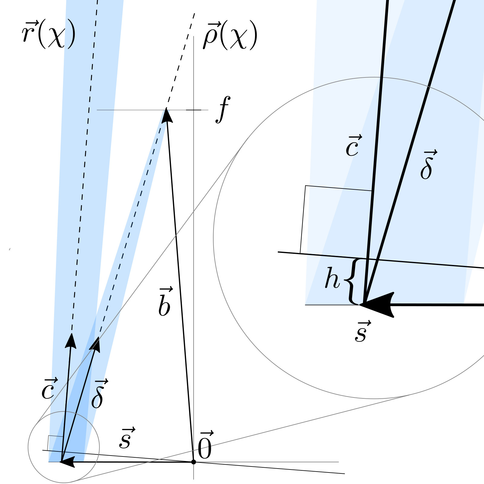
Figure 6: A dashed ray $\vec{r}(\chi)$ in its blue beam $\mathcal{B}{}$ and its corresponding dashed image ray $\vec{\rho}(\chi)$ in its own blue image beam $\mathcal{B}_{\text{img}}{}$. In the close-up, one can see the distance $h$ to correct the length of the optical path for ‘ideal’ timing. The construction of $\vec{b}$ is shown in  A.

4.1 Projecting the Plenoscope’s Response onto Images

One can project the response of the plenoscope’s $K$ photosensors $\mathcal{R}{}_{\text{h}}{}$ onto an image with $N$ pixels. Here, a pixel is just a picture-cell in a histogram over directions, and has no physical counterpart on the plenoscope. These pixels do neither need to have the shape of the plenoscope’s eyes, nor does their number $N$ need to match the number of eyes in the plenoscope. One can define the plenoscope’s image

$$\mathcal{I}{} = \begin{bmatrix}j_{1},j_{2},\dots j_{N}\end{bmatrix}.$$ (13)

as a list of $N$ intensities $j$.

For simplicity, we integrate over time here so that $\mathcal{R}{}_{\text{h}}{}$ lists only one intensity for each of the plenoscope’s $K$ photosensors.

Now, one can project the response $\mathcal{R}{}_{\text{h}}{}$ onto an image $\mathcal{I}{}_{g}$ which has its focus set to an arbitrary depth $g$ of one’s choice by multiplying

$$\mathcal{I}{}_{g} = U(g)\cdot\mathcal{R}{}_{\text{h}}{}$$ (14)

with the imaging matrix

$$U(g) = \begin{bmatrix}u_{1,\,1}(g)&u_{1,\,2}(g)&\ldots&u_{1,\,K}(g)\\ u_{2,\,1}(g)&u_{2,\,2}(g)&\ldots&u_{2\,K}(g)\\ \vdots&\vdots&\ddots&\vdots\\ u_{N,\,1}(g)&u_{N,\,2}(g)&\ldots&u_{N,\,K}(g)\\ \end{bmatrix}$$ (15)

which elements depend on the desired depth $g$. Once one knows an instrument’s light-field calibration $\mathcal{G}{}$, the computation of its imaging matrix $U(g)$ is straight forward as shown in  B.

4.2 Timing in Images

Timing in the regime of $1\,$ns is important to the atmospheric Cherenkov method to identify flashes of Cherenkov photons in between the other photons from the nightly sky. Optics effect this timing, and can induce undesired spreads when optical paths differ in length. A segmented mirror with its facets placed on a parabola has good timing in the center of its image. Only when such a mirror is large, and angles off its axis increase, the spread in time becomes relevant. For example: A parabolic mirror with $D=71$ m in diameter and a screen in $f=106.5\,$m focal-length induces a spread of $\approx 25\,$cm$\,{c_{0}}^{-1}\approx 0.8\,$ns in between the paths of two parallel running photons which are $3.25^{\circ}$ off the mirror’s optical axis and are being reflected on opposite edges of the mirror. On the plenoscope, one can resolve this spread in time. For this, one needs a model for ideal timing in an image. We define ideal timing such that photons, which travel in the same direction $\vec{c}$ (i.e. before they enter the instrument) and within a plane perpendicular to their direction of motion, are assigned to the same bin in time. Fig. 6 shows the distance

$$h = \vec{s}^{T}\cdot{}\vec{c}=s_{x}c_{x}+s_{y}c_{y}$$ (16)

between the point of the photon being closest to the aperture’s origin, and the point of the photon intersecting with the aperture’s principal plane. With this distance, and the time of the photon’s passing through the aperture’s principal plane in Eq. 10, one can compute the photon’s time of arrival

$$t_{\text{img}} = t_{\text{aperture}}+h\frac{n}{c_{0}}$$ (17)

in a sequence of images. The speed of light $c_{0}$ and the medium’s refractive index $n$ match Eq. 11.

This means that when an instrument records a sequence of images over time (i.e. a movie), then the moment $t_{\text{img}}$ in this sequence to which the photon must be assigned to is defined as the moment when the photon would have been closest to the central point of the instrument’s aperture, if nothing was ever stopping the photon on its initial trajectory coming down from the sky.

Correcting the timing becomes relevant when the parabolic mirror deforms, or if one wants to use a different design for the segmented mirror in the first place. For example, the plenoscope can reduce the spread in time induced by a mirror with Davies and Cotton (1957) design, which otherwise becomes significant for diameters beyond $D\approx 15\,$m.

5 Introducing Portal

Portal is a specific Cherenkov plenoscope designed to detect cosmic gamma rays with energies as low as 1 GeV in an effective collecting area of several 10³ m². Here we motivate Portal’s design from the optics point-of-view and demonstrate its powerful perception of depth and its ability to compensate aberrations, deformations, as well as misalignments. Together, we designed Portal’s mechanical structure in an interdisciplinary collaboration of civil engineering and particle physics (Daglas, 2017, Zinas and Daglas, 2016).

5.1 Overview

Fig. 7 shows Portal with its two main components, first its imaging mirror, and second its light-field camera. Plenoptic’s relaxed constrains for rigidity and alignment allow Portal to mount its mirror and its camera independently on two mounts. The first mount moves the mirror which has a diameter of $D=71\,$m, a focal-length of $f=106.5\,$m, and a focal-ratio of $F=1.5$. The second mount moves the light-field camera which has a diameter of $12.1\,$m corresponding to a field-of-view of $6.5^{\circ}$. All optical surfaces are spherical to ease fabrication. All of Portal’s optics are made from only two repeating primitives to ease mass production: One reflective facet for the mirror, and one transparent lens for the eyes in the light-field camera. The primitives are truly identical so that any facet can replace any other facet, and any lens can replace any other lens. Portal’s mounts are actuated by cable robots (Miermeister et al., 2016) which can point Portal up to $45^{\circ}$ away from zenith and have only cables shadowing the mirror. When hunting flares and bursts of gamma rays, Portal points with an estimated $90^{\circ}$ min^-1 and can always move along the shortest route along the great circle because unlike the altitude-azimuth mount (Borkowski, 1987) Portal’s kinematic has no singularity near the zenith. To keep the mounts small, the mirror moves in one direction while the camera moves to the other what effectively rotates the unity of mirror and camera around its common center. During the day, the light-field camera parks on a pedestal to the side to ease service, while the mirror parks flat on the ground.

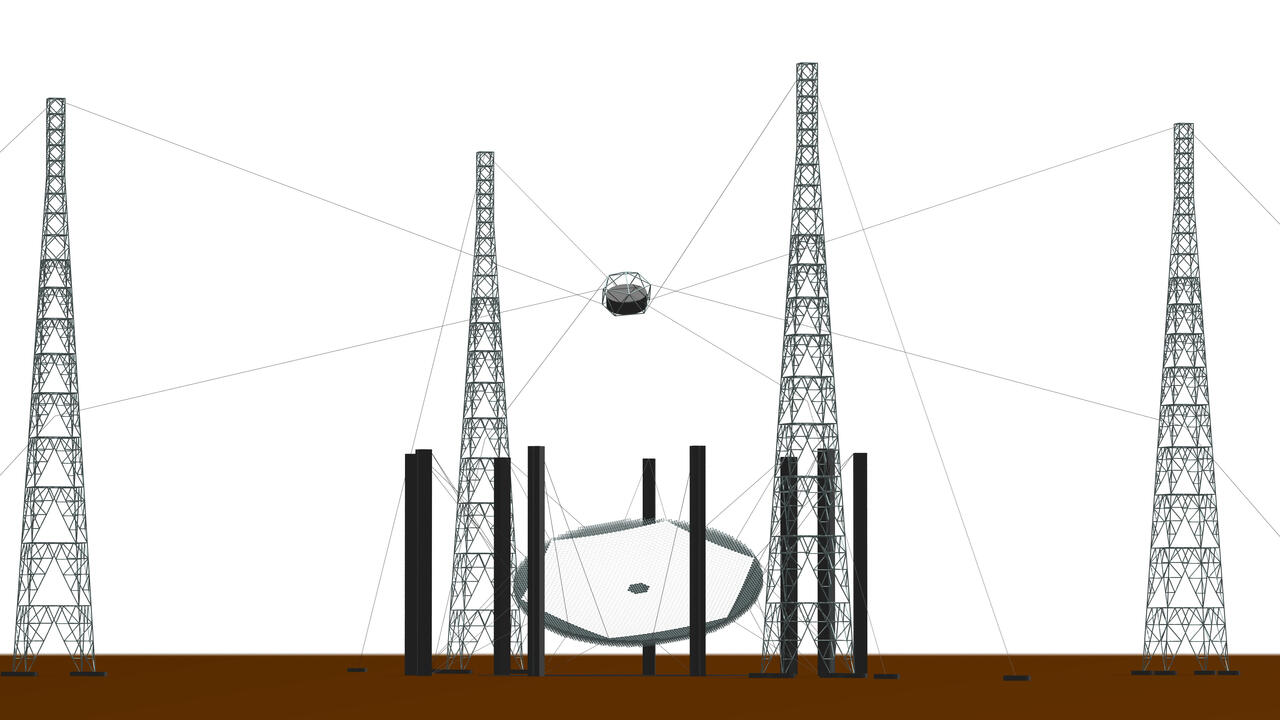
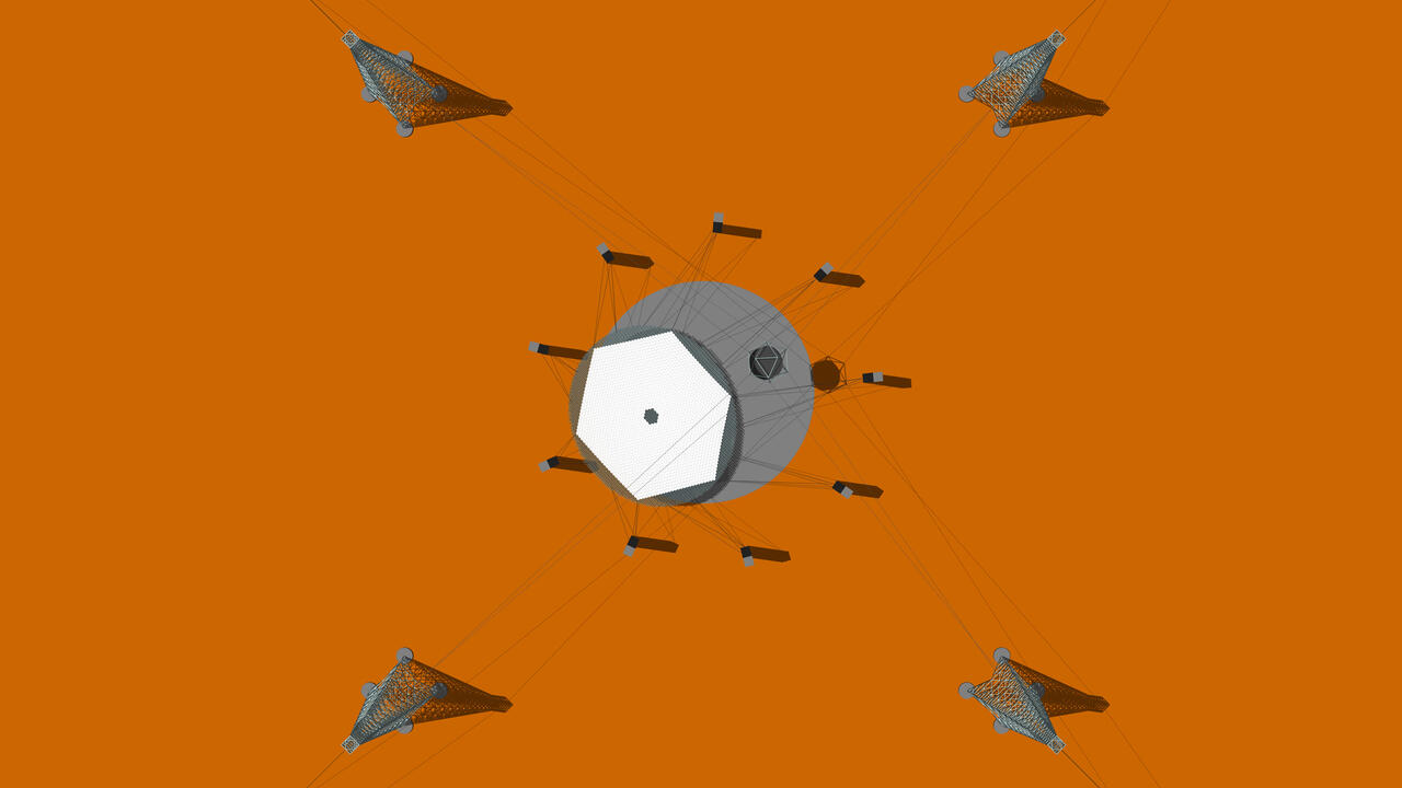
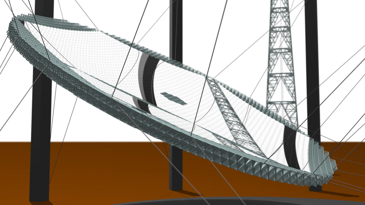
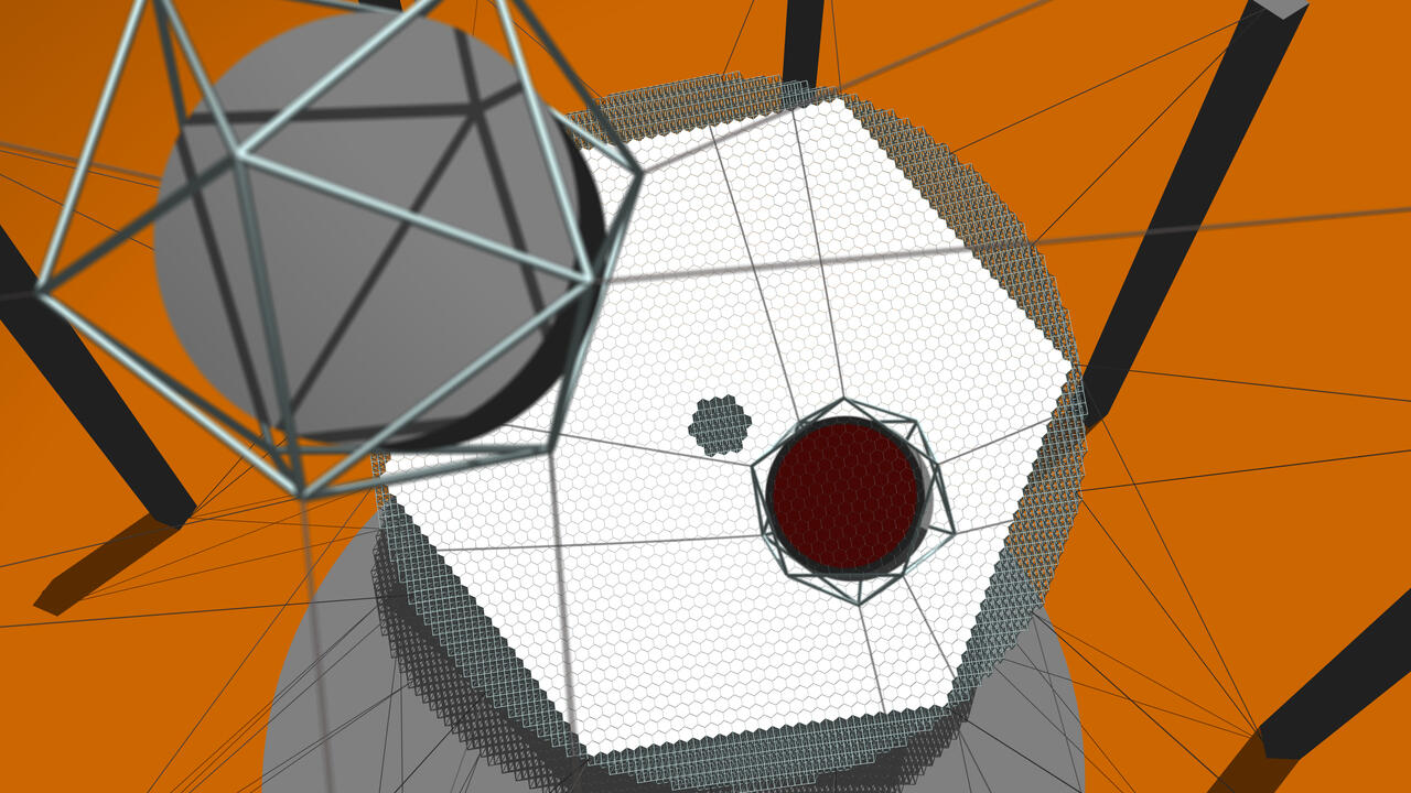
Side from a distance. Top from a distance. Mirror with own mount suspended from cables. light-field camera above mirror.

Figure 7: The Portal Cherenkov plenoscope with its two independent mounts for the mirror and the light-field camera. Renderings similar to Mueller (2019) (mirror is different).

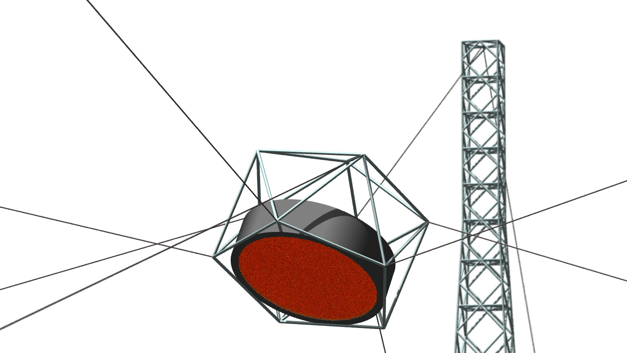
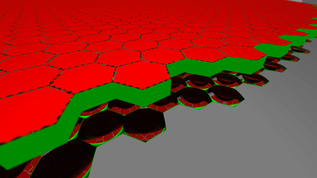
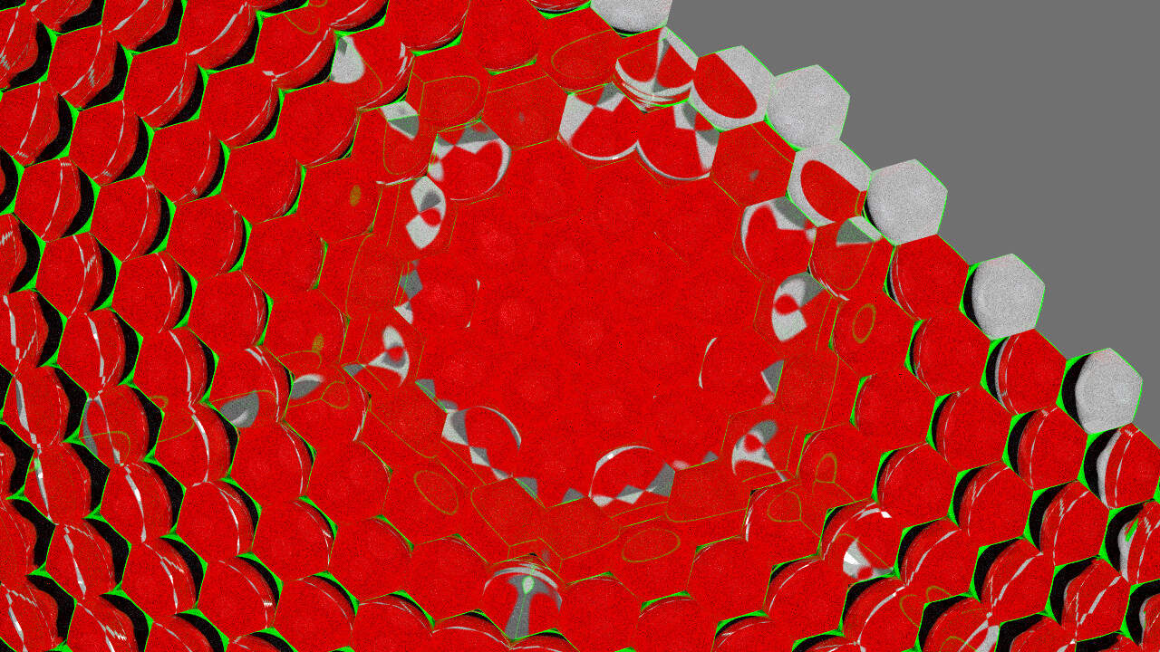
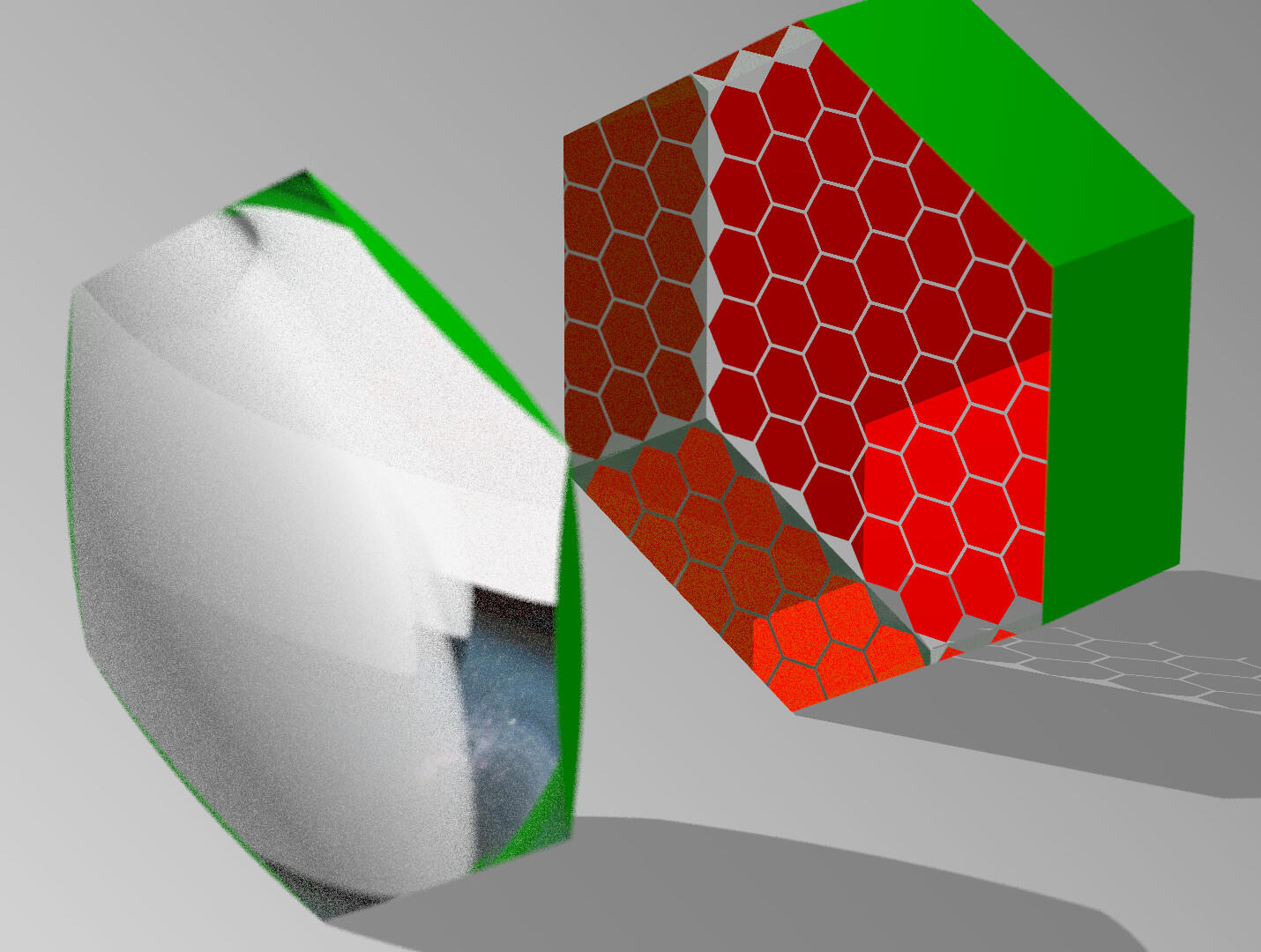
light-field camera with own mount suspended from cables. Inside light-field camera, array of eyes. Below light-field camera, looking up into the eyes lenses. Single eye taken from light-field camera.

Figure 8: Portal’s light-field camera in more detail. Renderings similar to Mueller (2019).

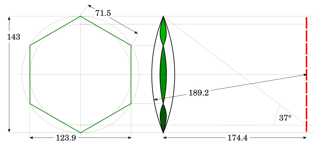
Figure 9: An eye in the light-field camera. The lens’ refractive index is $\approx 1.47$ for a wavelength of $400\,$nm. Left: Front-view. Right: Side-view. The photosensors are red and the opaque faces of the lens are green. Dimensions / mm. Adopted from Mueller (2019).

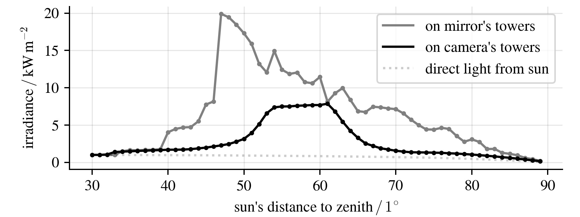
Figure 10: The worst case irradiation from reflected sunlight found in hot spots on Portal’s towers when the mirror has its facets perfectly aligned and is parking flat on the ground.

5.2 Light-Field Camera

Fig. 8 shows Portal’s light-field camera which is a dense array of $N=8,443{}$ identical eyes arranged in a hexagonal grid. The camera’s field-of-view spans $6.5^{\circ}$ on the sky, what corresponds to a diameter of $\approx 12.1\,$m. A single eye’s field-of-view spans $0.067^{\circ}$ on the sky, what is on a par with existing Cherenkov telescopes (Cornils et al., 2005). Each eye is made out of a bi-convex, spherical lens and an array of $M=61{}$ photosensors encased in a hexagonal cylinder, see Fig. 9. Thus Portal’s light-field camera has a total of $K=M\times N=515,023{}$ beams. In general, the lens’ focal-ratio must match the mirror $F\geq F_{\text{lens}}$, in order to have the lens’ image of the mirror fully contained within the eye’s body. In Portal the lens’ focal-ratio is $F_{\text{lens}}\approx{}1.4$ to ensure the lens’ image of the mirror is a bit smaller than the eye’s body. This way the array of photosensors inside the eye does not need to cover the full cross-section of the eye and instead can leave space for the walls of the eye’s body. Since the eye’s body is hexagonal, the array of photosensors inside the body is also a hexagon. This in turn allows the lens’ image of the mirror to be hexagonal which motivates the hexagonal outer shape of Portal’s mirror. The inner walls of the eye’s hexagonal body reflect light, at least a part of the wall close to the photosensors. This is because the lens refracts parts of the light coming from the outer parts of the mirror too far off its optical axis. We found that making the flat inner walls reflective helps to redirect this light mostly back into the photosensors which are meant to receive it in the first place.

At the time of writing, the area of photosensors, and to some lesser extent the number of read-out channels inside the light-field camera seem to determine Portal’s costs. This assessment is motivated by our early listing of Portal’s costs (Mueller, 2019), which includes listings of the cable-robot mount and the support structure (Daglas, 2017).

5.3 Mirror

Portal’s mirror is a dense array of $1,842{}$ identical, reflective facets arranged in a hexagonal grid. Each facet’s spherical surfaces has a radius of curvature of $2f$, and an area of $\approx 2\,$m², what is common on large Cherenkov telescopes (Pareschi et al., 2013). The inner, flat-to-flat diameter of the hexagonal facets is $1,500\,$mm and the gap between the facets is $25\,$mm. The outer perimeter of the mirror is a hexagon to fill the photosensors in the eyes, see in Sec. 5.2. The facets centers are on a parabola with focal-length $f$.

The quality of the facets surfaces does not need to exceed the quality of the surfaces used in existing Cherenkov telescopes. On most Cherenkov telescopes, the quality of the facets surfaces allows the telescopes to concentrate parallel light, from e.g. a star, into an area on their camera’s screen which feeds only into a single photosensor (a single directional bin on the telescope). Similar on the plenoscope, the quality of the facets surfaces must only be good enough to concentrate parallel light into the lens of a single eye (a single directional bin on the plenoscope). On both the telescope and the plenoscope, the exact position where a photon enters a directional bin (e.g. a light-guide on the telescope or an eye’s lens on the plenoscope) is not relevant. In case of the plenoscope’s eye, this is because the eye’s lens is an imaging optics itself which can be described with Fig. 4 and Eq. 1. This means that a photosensor inside the eye receives light from only one specific direction relative to the lens, but from any possible impact position on the lens. So as the position where light passes through an eye’s lens does not matter, the mirror facets for the Cherenkov plenoscope do not need to exceed the surface quality of existing mirrors on Cherenkov telescopes.

Because of the many facets, Portal adopts the established alignments of Cherenkov telescopes which: First, measure all the facet’s orientations in parallel (McCann et al., 2010, Ahnen et al., 2016b). And second, adjust all the facet’s orientations in parallel with an active mirror control (Biland et al., 2007).

5.4 Estimating the Light-Field Calibration

Estimating Portal’s light-field calibration with simulations is straight forward, and simulations of optics are well established (Bernlöhr et al., 2013, Okumura et al., 2016) in the atmospheric Cherenkov method. But simulations depend on how well one can measure the plenoscope’s geometry. To ease this, Portal takes two measures:

First, Portal’s mechanical structures are designed to deform steady and reproducible with respect to the pointing (Daglas, 2017). This makes it easier to estimate the plenoscope’s geometry from fewer position sensors, and allows to interpolate between estimates. Large Cherenkov telescopes already use such designs to ease the alignment of their mirror’s facets (Biland et al., 2007).

Second, Portal measures the shape of its mirror using the response of its photosensors to a known source of light. The idea is inspired by Cherenkov telescopes which use CCD cameras and the light of a star to measure the normal vectors on the surface of a mirror in great detail (Arqueros et al., 2003, McCann et al., 2010, Ahnen et al., 2016b). When involving the eyes in Portal’s light-field camera directly, deformations of the mirror with low spatial frequencies can be kept track of during regular observations.

5.5 Estimating the Risk from Sunlight

An active mirror control can also misalign the facets to prevent the mirror from focusing sunlight onto its surrounding. Depending on the location on earth, the mirror can also park inclined away from the sun to further minimize the risk from focused sunlight. In the worst case when the mirror parks flat on the ground and its facets are well aligned the ground is still safe but reflected sunlight will reach the surrounding towers, see Fig. 10. This worst case irradiance of 20 kWm^-2 needs to be addressed with passive protection and access limitations on some of the towers, but is still more than a factor of 200 below the irradiance found in solar concentrators (Dibowski et al., 2023).

5.6 Imaging

Fig. 11 visualizes the elements of matrix $U(g)$ from Eq. 15 on the Portal Cherenkov plenoscope. Here in this demonstration, we set the binning of the pixels in the final image so that the central pixel falls together with the central eye in Portal’s light-field camera. The final image itself is not shown here, but one finds that in this special case all the photosensors of an eye contribute to the same pixel. At least when the pixel is close to the mirror’s optical axis where aberrations are low, and when the image’s focus corresponds to the camera’s focus. This very special case is the upper panel in Fig. 11. When the final image changes its focus, one finds that photosensors from multiple eyes contribute to a pixel. This is what the lower panels in Fig. 11 show. One finds that photosensors which contribute to the same pixel are in close, mechanical proximity. This proximity can be minimized when the camera’s focus corresponds to the final image’s focus. In the field, one would focus the light-field camera to the average depth of the showers one wants to record to minimize this proximity. Minimizing this proximity eases the implementation of fast imaging close to the hardware. And fast imaging is relevant for the trigger.

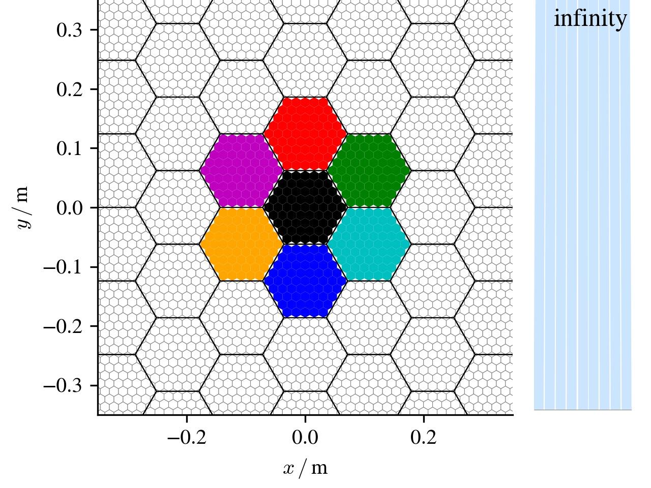
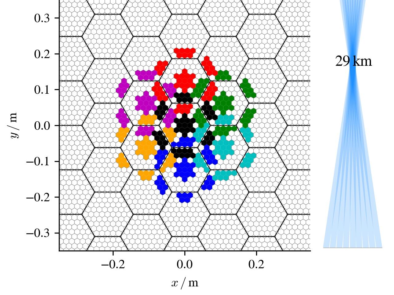
Figure 11: A close-up on the photosensors in Portal’s light-field camera. Large hexagons are eyes. Small hexagons are photosensors. Seven colors correspond to the seven central pixels of the final image. Three panels show the final image’s focus set to different depths in $g=(\infty{}$, 29 km, 21 km). Compare Fig. 17b which also shows $U(g)$, but for larger angles off the mirror’s optical axis. State of Portal: (mirror: good, camera: good).

5.7 Trigger

Portal adopts two powerful concepts from the Cherenkov telescope’s trigger. First, it acts on an image, and second it sums up the signals of multiple photosensors (Garcia et al., 2014) to reduce accidental triggers. To provide the trigger with an image, Portal’s light-field camera continuously projects its light field onto an image. Eq. 14 shows how this projection is implemented in hardware as the matrix’s elements $u_{n,\,k}(g)$ mask if a photosensor $k$ contributes its signal to the sum of pixel $n$ or not. Inside the light-field camera are $N_{\text{trigger}}$ hubs which sum the signals of specific photosensors. These hubs are evenly spread in between the light-field camera’s eyes and represent the $N_{\text{trigger}}$ pixels of the trigger’s image. Each hub runs signal routes according to matrix Eq. 15 to specific photosensors. Due to the plenoscope’s design, these photosensors are already in the mechanical proximity of the hub, see Fig. 11, and do not require to be delayed in time for different pointings. This way from a signal-processing point-of-view, Portal’s trigger is a sum trigger that acts on an image exactly the way a Cherenkov telescope’s sum trigger acts.

In addition the plenoscope’s trigger can be extended to perceive depth. To do so, Portal’s trigger projects its light field not only onto one, but onto two images. By installing the hubs for summation twice, but applying two different imaging matrices $U(g_{\text{far}})$, and $U(g_{\text{close}})$, Portal’s trigger acts on two images. The far image focuses on the depth $g_{\text{far}}$, and the close image focuses on the depth $g_{\text{close}}$. With this perception of depth, Portal can trigger faint showers exclusively when they emit their light high up in the atmosphere (far image), what is typical for low energetic gamma rays. This way, and on a statistical basis, Portal’s trigger can be made to favor low energetic gamma rays over faint sources that emit their light further down in the atmosphere, such as parts of hadronic showers impacting at large distances.

5.8 Optical Performance

We will discuss Portal’s point-spread-function for imaging in the following sections but because images are only projections of light fields we first want to look at the beams which sample this light field. A simple characterization of the $k$-th beam $\mathcal{B}{}_{k}$ is its spread in solid angle in the sky $\Omega{}_{k}$, its spread in area on the aperture’s principal plane $A{}_{k}$, its spread in time that can not be resolved $T{}_{k}$, and its optical efficiency $E{}_{k}$. Fig. 12 shows the distributions of these spreads for Portal, and  C shows how we define those. In summary: Portal’s beams resolve solid angles of 1.8 $\mu$sr, (a cone with an half-angle of $0.043^{\circ}$), they resolve areas of $160\,$m² (a disk of $14.3$ m in diameter) on the aperture’s principal plane, they induce an unresolvable spread in time of $0.4\,$ns, and their optical efficiencies are rather similar. The clusters in the beams efficiencies in Fig. 12 change with the camera’s alignment and the mirror’s shape and are caused by the camera shadowing the center of the mirror.

The plenoscope’s performance to perceive depth illustrates the overlap of its beams. Fig. 13 shows how the blur in an image of a point like source changes when the focus of the image changes. Indeed, Fig. 13 shows this for eight isolated sources which where observed independently. One finds that the focus with the minimal spread is a good estimator for the true depth of the source. Fig. 14 histograms the confusion of many of such estimates where a source is observed and has its depth reconstructed by Portal minimizing the spread in its refocused image. The sources are randomly placed in a depth ranging from $2\,$km to $40\,$km and are uniformly distributed in Portal’s field-of-view. In the histogram one finds Portal’s confusion to show more at further depths, as one would expect from any stereoscopic observation with a finite baseline, and as the range $(g_{+}-g_{-})$ in Eq. 2 predicts it. Still, the range in depth with good resolution comfortably covers a typical shower induced by a cosmic gamma ray.

But keep in mind that Fig. 13 and Fig. 14 show the case of observing a bright point like source what gives better performance than what is to be expected from the reconstruction of an actual shower, initiated by a 1 GeV gamma ray, which emits less Cherenkov photons and is more spread out in space. Similar to the telescope’s point-spread-function, which is also showing a bright point like source, it might be good to interpret Fig. 13 and Fig. 14 as the plenoscope’s ‘depth-spread-function’.

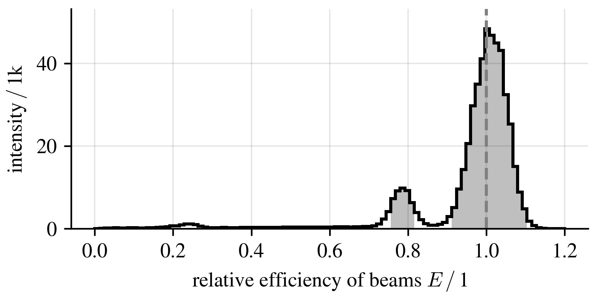
Figure 12: Statistics of Portal’s $K$ beams gathered from its light-field calibration $\mathcal{G}{}_{\text{default}}$ when Portal is in its default geometry, i.e. Portal’s mirror is not deformed and its light-field camera is both centered on, and orientated perpendicular to the mirror’s optical axis. Dashed, vertical, gray line is the median. Light gray areas show the $90\%$ percentile. Statistics is $\approx 1000$ optical paths per beam. Compare  C, Eq. 29 to Eq. 32. State of Portal: (mirror: good, camera: good).

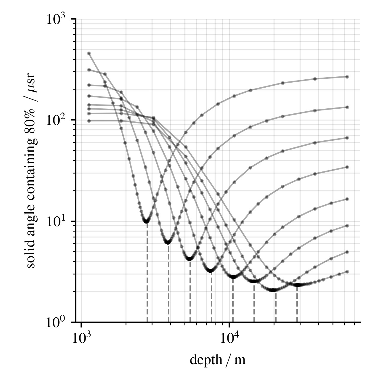
Figure 13: Portal observes eight isolated point like sources in eight different depths. Each solid line is one observation and the dots indicate projections of the observed light field onto an image focusing to a specific depth. The dashed vertical lines indicate the true depth of the point like sources. State of Portal: (mirror: good, camera: good).

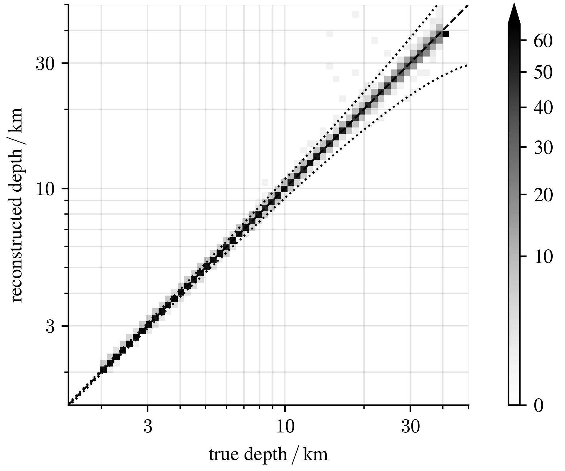
Figure 14: Portal’s confusion in depth for isolated point like sources randomly scattered in depth and directions (across Portal’s field-of-view). Dotted lines show Portal’s $g_{-}$ and $g_{+}$ according to Eq. 2. State of Portal: (mirror: good, camera: good).

5.9 Comparing to a Telescope, and to a Variant

To compare the Portal Cherenkov plenoscope to a telescope, we introduce a Cherenkov telescope named ‘P-1’. The difference between P-1 and Portal is in how well they can resolve the position where a photon is reflected on their mirrors. The P-1 telescope naturally resolves its mirror in only 1 bin, hence the ‘1’ in P-1. The Portal plenoscope resolves its mirror in 61 bins because its eyes have 61 photosensors each. One might refer to Portal as ‘P-61’ in this scheme. To further demonstrate how this resolution impacts plenoptic perception we also introduce a plenoscope ‘P-7’ which is also identical to Portal except for it only has 7 bins to resolve its mirror. To make a fair comparison, we estimate the light-field calibration for each instrument, including P-1, and apply it to compute images. This way, the few effects that a telescope can compensate (distortion, vignetting, specific misalignments) are taken care of equally for every instrument.

In addition, one wants to adjust the focus of the telescope P-1, such that its images of stars are sharp. This is because when we will compare the variants (P-1, P-7, and P-61), we will use star light. Since Portal can compensate translations of its camera relative to its mirror, this adjustment of the focus is not important for the Portal (P-61) plenoscope. But for the telescope P-1, adjusting the focus is important (Trichard et al., 2015, Hofmann, 2001). When searching for the highest concentration of star light from Portal’s mirror, one finds that the focal-point, which one estimates this way, is $1.66$ m closer to the base of the mirror’s parabola than the parabola’s theoretical focal-point. After all, segmented mirrors with facets on a parabola are not the same as parabolic mirrors. To account for this, one translates the cameras screens of all variants (P-1, P-7, and P-61) into this estimated focal-point, and orientates the camera’s screen to be perpendicular to the mirror’s optical axis. For reference, we mark this using the expression ‘camera: good’ wherever it is applicable, see e.g. Fig. 15.

With the estimated focal-point, one also found the aperture’s principal plane of Portal’s mirror which is located $1.66$ m below the mirror’s parabola which mounts the facets. When one estimates the light-field calibration for the variants (P-1, P-7, and P-61), one uses this estimated principal plane together with the optical axis as the frame of reference, compare Sec. 3.1.

6 Compensating Aberrations

Real mirrors induce aberrations in images. In Cherenkov telescopes, the mirror’s aberrations limit the field-of-view as its blurring gets stronger with larger angles off the mirror’s optical axis. A significant enlargement of the field-of-view is currently only possible when concatenating aspheric, and non-flat optical surfaces (Vassiliev and Fegan, 2007). Fig. 15 shows the reconstructed images of a star observed by the Portal plenoscope and the telescope P-1 for three different angles off the mirror’s optical axis. The images are computed according to Sec. 4.1. Both telescope and plenoscope offer a small point-spread-function in the center of the field-of-view, but for larger angles off the mirror’s optical axis, the blurring in the telescope’s image increases rapidly. On the other hand, the Portal plenoscope’s point-spread-function is hardly effected by the light’s direction. Fig. 16 shows how the plenoscope’s and the telescope’s point-spread-functions scale with the light’s angle off the mirror’s optical axis. On average across the field-of-view, the telescope P-1 contains 80% of the light from a star in a cone with a solid angle of 12 $\mu$sr (half-angle 0.11^∘). The Portal plenoscope contains the same light in a quarter of the solid angle of 3.2 $\mu$sr (half-angle 0.058^∘). By means of the atmospheric Cherenkov method, Portal’s images are very sharp and very ‘flat’ i.e. very independent of the direction of the light.

Telescope P-1
Plenoscope P-7
Portal Plenoscope P-61

Figure 15: Images of a star for three angles off the optical axis taken by the three tele- and plenoscopes P-1, P-7, and P-61 while all optics have their targeted geometry: (mirror: good, camera: good). Fig. 16 shows the corresponding spread averaged over many stars.
Legend: The three columns show the star being 0.0^∘, 1.5^∘, and 3.0^∘ off the mirror’s optical axis. Axes are in units of $1^{\circ}$. The little hexagon shows the field-of-view of a telescope’s photosensor and plenoscope’s eye respectively. The dashed ring shows the containment of 80% of the star’s light. The big ring in the most right panels shows the limit of the instrumented field-of-view.

Figure 16: The spread of a star’s image vs. the star’s angle off the optical axis for the three tele- and plenoscopes P-1, P-7, and P-61 while all optics have their targeted geometry: (mirror: good, camera: good). Fig. 15 shows corresponding example images of the star.
Legend: Stars are randomly placed in the sky. The stars are binned according to their angles off the optical axis. The bins cover equally large solid angles. The lines show the average spread of the stars images within a bin.

To visualize how Portal compensates the aberrations one can again color the elements of the imaging matrix $U$ for certain pixels, see. Fig. 17a, and Fig. 17b. One finds that the aberrations of Portal’s mirror are small when close to the optical axis (A), but become stronger the further the light is off the optical axis (F). The aberration’s spread becoming stronger with larger angles corresponds to the growing distances between the colored photosensors. Just like in Fig. 11, in the special case of the pixel being on the mirror’s optical axis the summation of photosensors simply runs over the central eye, see panel (A) in Fig. 17b.

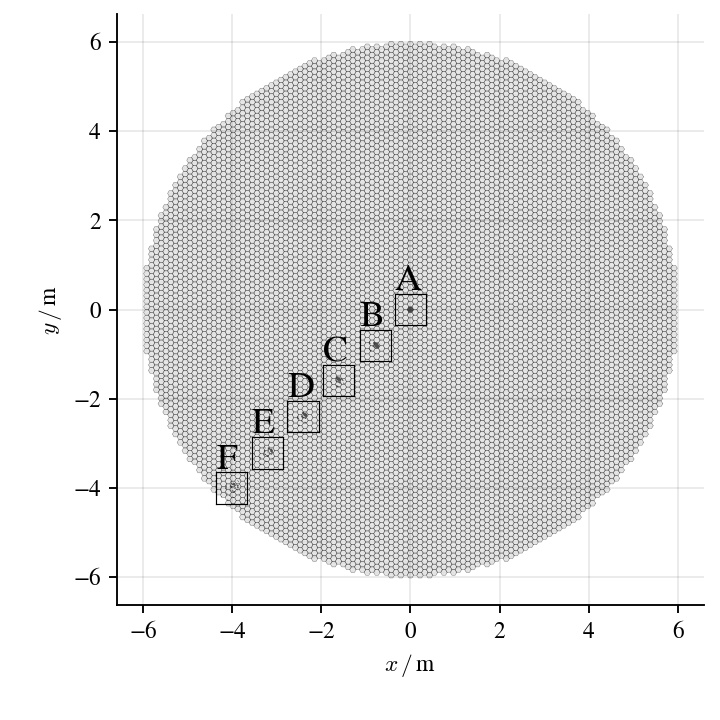
(a)

(b)

Figure 17: The pixels angles off the mirror’s optical axis are: A: 0.0^∘, B: 0.6^∘, C: 1.2^∘, D: 1.8^∘, E: 2.4^∘, and F: 3.0^∘. Dark photosensors show the non-zero elements in the rows of the imaging matrix $U(g)$ in Eq. 15. State of Portal: (mirror: good, camera: good).

7 Compensating Deformations

Deformations in the mirror’s supporting structure effect the normal vector of the mirror’s surface. Deformations induce aberrations which blur the image. However, a plenoscope can compensate such deformations when the deformation’s spatial frequencies across the mirror are low enough. Deformations with spatial frequencies lower then the spatial resolution a plenoscope has to resolve its mirror do only re-orientate the plenoscope’s beams but they do not widen the plenoscope’s beams. And as long as the beams are not widened, the plenoscope’s performance is hardly reduced. To demonstrate plenoptic’s capabilities to compensate such deformations we compare Portal’s images to the images taken by the telescope P-1. All instruments use identical mirrors with the deformation shown in Fig. 18. We deform the mirror randomly using Perlin (1985) and set the magnitude such that some of the mirror’s facets deviate from their targeted orientations by $0.12^{{}^{\circ}}$. For a telescope, where the field-of-view of a pixel is $0.067^{\circ}$, such a deformation is significant as it potentially spills light from a star over several neighboring photosensors in the telescope’s image camera. Fig. 19 shows the images of a star taken by the different instruments for three different angles, and Fig. 20 shows how the spread of the images changes with the star’s angle off the optical axis. As expected, the telescope’s image is significantly washed out and it takes a solid angle of $\approx 53\,\mu$sr (half-angle: 0.23 ^∘) to contain 80% of the light. In contrast, the Portal Cherenkov plenoscope reduces the 80%-cone’s solid angle by almost one order of magnitude down to only $\approx 6.1\,\mu$sr (half-angle: 0.08 ^∘).

Since the Cherenkov plenoscope can compensate deformations after it has recorded a shower, it can compensate deformations as rapidly as it can measure them. Rapid deformations might be caused by gusts of wind or by a fast pointing in order to hunt a transient source of gamma rays. On a structure with the size of Portal, distance- and angle-sensors can sample with rates in a regime of several $10$ s^-1 what allows to compensate changes in the mirror’s deformation with frequencies as high as several $1$ Hz. The plenoscope’s rapid compensation of deformations is a powerful augmentation to the precise, but gentle, re-orientation of facets in a Cherenkov telescope’s active mirror control (Biland et al., 2007) which in the end is also subject to mechanical wear and tear. Combining the two approaches covers a wide range of scenarios and makes the Portal Cherenkov plenoscope promising to choose a more forgiving, more elastic, and thus less expensive design for its mirror. Although the plenoscope’s light-field calibration will allow the compensation of a broad range of deformations in the mirror, Portal still has an active mirror control because it eases the initial alignment of the many facets, and because it can reduce the risk of having concentrated sunlight, see Sec. 5.5.

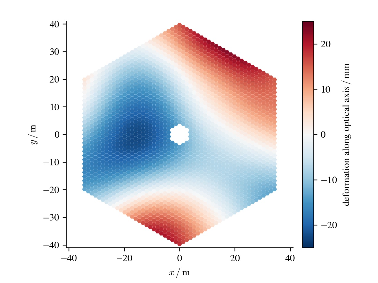
Surface’s height along the optical axis. Surface’s normal vector.

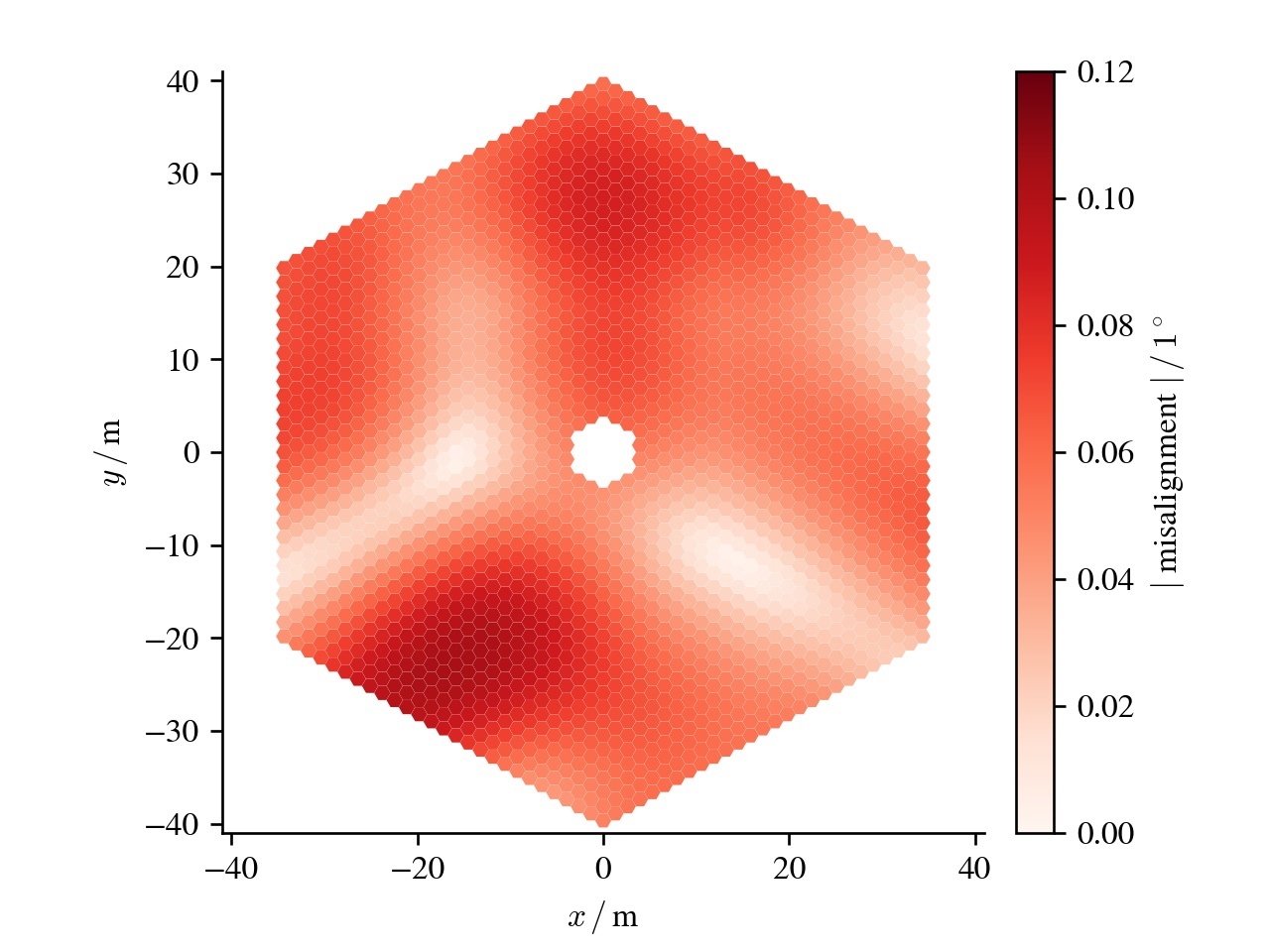
Figure 18: Deformations in the mirror effect its surface’s normal vector.

Telescope P-1
Plenoscope P-7
Portal Plenoscope P-61

Figure 19: Images of a star for three angles off the optical axis taken by the three tele- and plenoscopes P-1, P-7, and P-61 while their mirrors are deformed: (mirror: deformed, camera: good). Fig. 20 shows the corresponding spread averaged over many stars. Find legend in caption of Fig. 15.

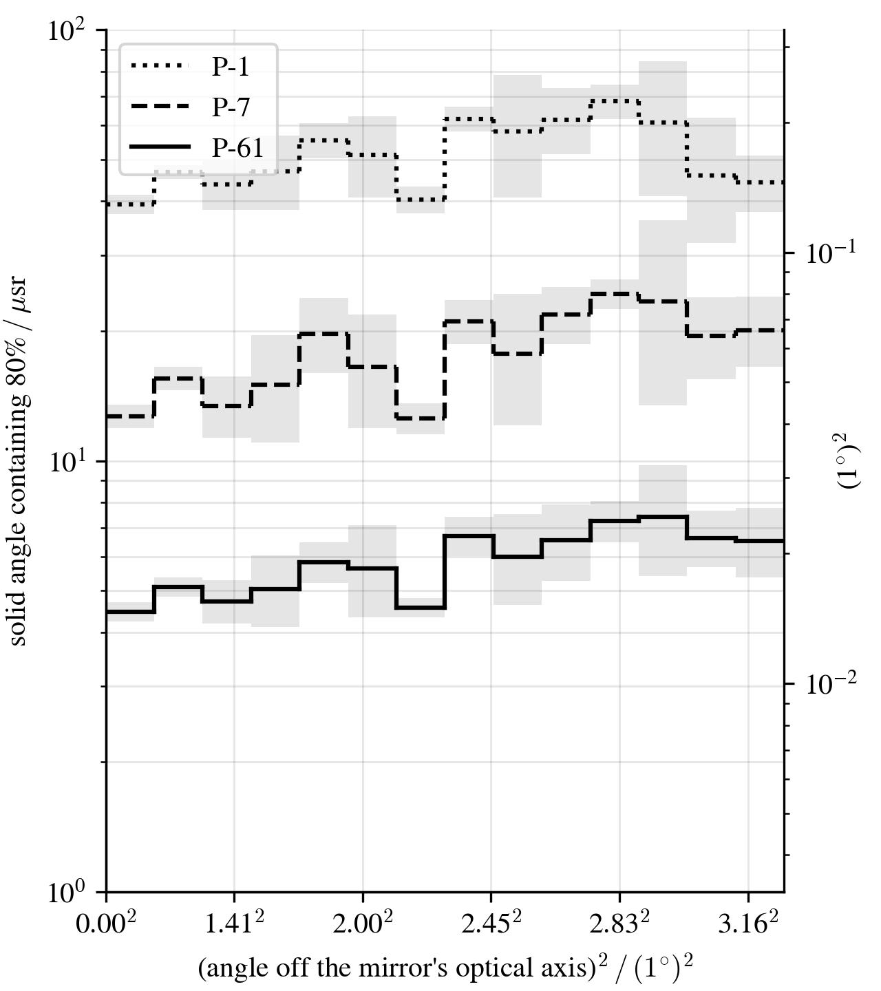
Figure 20: The spread of a star’s image vs. the star’s angle off the optical axis for the three tele- and plenoscopes P-1, P-7, and P-61 while their mirrors are deformed: (mirror: deformed, camera: good). Fig. 19 shows corresponding example images of the star. Find legend in caption of Fig. 16.

8 Compensating Misalignments

The prevention of misalignments between a telescope’s mirror and its camera rapidly complicates the construction of larger telescopes. While a telescope can compensate certain components of misalignments when these are known, others blur its image irrecoverably. Tab. 1 shows that the telescope P-1 can tolerate absolute misalignments in the regime of $10^{-3}\,f$ before its image degrades significantly.  D shows how we estimate these tolerances. The components of misalignment which the telescope can not compensate make independent mountings of the mirror and the camera impractical. A rigid mechanical support is required between the mirror and the camera to prevent misalignments in the first place. The plenoscope relaxes this limitation as it can compensate all components of a misalignment. To demonstrate the plenoscope’s power to compensate misalignments we significantly misalign the camera on purpose, see Tab. 2. Fig. 21 and Fig. 22 show the images of stars taken with the camera being misaligned. Since we apply the light-field calibration also to the images of the telescope P-1, the components of misalignment which the telescope P-1 can compensate for, are compensated for. This is why the average of the star’s light is reconstructed with its correct direction in the images of P-1. But the large spread of the stars in P-1’s images shows that we pushed the telescope P-1 beyond its limits. In contrast, the misaligned Portal plenoscope provides images which still outperform the images of the telescope P-1 when P-1’s camera is perfectly aligned, compare Fig. 16 and Fig. 22.

	tolerance when not	can be compensated
	compensated for	telescope	plenoscope
	Translating parallel
	$\Delta_{\parallel}\approx\pm 96\,$mm $\approx 10^{-3}\,f$	No	Yes
	Translating perpendicular
	$\Delta_{\perp}\approx\pm 63\,$mm $\approx 10^{-3}\,f$	Yes⋆	Yes
	Rotating parallel
	$\Phi_{\parallel}\approx\pm 0.59^{\circ}$	Yes	Yes
	Rotating perpendicular
	$\Phi_{\perp}\approx\pm 0.83^{\circ}$	No⋆⋆	Yes

Table 1: The four components of misalignments between a camera and a mirror. The tolerances are estimated for the telescope P-1. (^⋆ Aberrations increase with the angle off the mirror’s optical axis. ^⋆⋆ The axis of the rotation forms a line across the camera’s screen which remains in focus and thus will not be blurred. But the rest of the image will be. ).

	component	absolute	relative
	Translating parallel
		-532.5 mm	5.5 $\Delta_{\parallel}$
	Translating perpendicular
		223.6 mm	3.5 $\Delta_{\perp}$
	Rotating parallel
		5.0 ∘	8.5 $\Phi_{\parallel}$
	Rotating perpendicular
		3.2 ∘	3.9 $\Phi_{\perp}$

Table 2: The misalignment of Portal’s camera in our demonstration. Explicit: Translation-$xyz$: (-100, 200, -532.5) mm, rotation tait-bryan-$xyz$: (1.0, 3.0, 5.0)^∘.

Telescope P-1
Plenoscope P-7
Portal Plenoscope P-61

Figure 21: Images of a star for three angles off the optical axis taken by the three tele- and plenoscopes P-1, P-7, and P-61 while their cameras are misaligned: (mirror: good, camera: misaligned). Fig. 22 shows the corresponding spread averaged over many stars. Find legend in caption of Fig. 15.

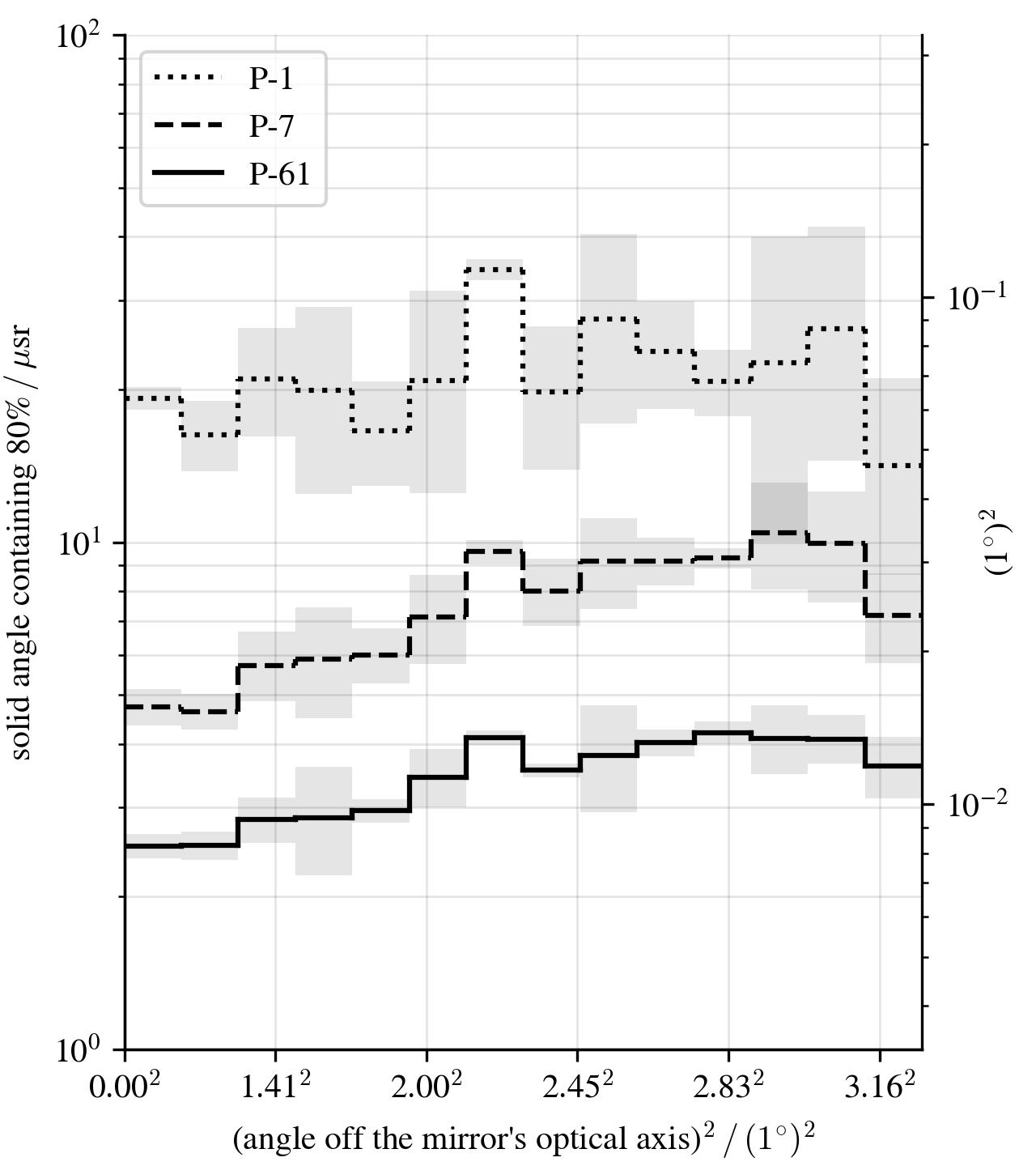
Figure 22: The spread of a star’s image vs. the star’s angle off the optical axis for the three tele- and plenoscopes P-1, P-7, and P-61 while their cameras are misaligned: (mirror: good, camera: misaligned). Fig. 21 shows corresponding example images of the star. Find legend in caption of Fig. 16.

9 Observing a Phantom Source

The observation of a phantom source in the atmosphere can demonstrate how efficiently the Cherenkov plenoscope can compensate aberrations, deformations in the mirror and misalignments of the camera. Fig. 23 shows the phantom source. Instead of a shower induced by a cosmic particle this phantom source is composed of structures which are easy to identify in an image, and which allow the viewer to formulate a well defined expectation of what the images should look like. The phantom source ranges from $2.5\,$km to $20.0\,$km in depth what matches the depth where most showers reach their maximum emission of Cherenkov light. Both the telescope P-1 and the Portal plenoscope observe the source. The geometries of both the telescope and the plenoscope do not change during the observation, and thus neither the telescope nor the plenoscope can physically adjust its focus, just as if they observe a flash of Cherenkov light. Fig. 24 shows the observations of P-1. One might argue that P-1’s physical focus is not set properly to any of the structures in the phantom source what prevents P-1 from producing a sharp image of at least one structure in the phantom source. But this is just what a narrow depth-of-field is all about: A large telescope like P-1 is unlikely to have a structure of interest in its narrow focus. In the images made by P-1 the triangle structure is blurred beyond recognition. By chance the cross structure and the letter-‘A’ structure are closest to the focus. Yet despite the blurring caused by the narrow depth-of-field aberrations can be found as the structures are not completely flat, i.e. their sharpness depends on where they are in the image.

Fig. 25 shows the observations of the Portal Cherenkov plenoscope (P-61). Portal projects its recorded light field onto images with different foci. The five images minimize the spread of individual structures of the phantom source. This way Portal estimates the depth of these structures, compare Fig. 13. The images show that despite deformations and despite misalignments Portal’s images are very flat. For most showers induced by cosmic particles, this is enough range in depth to refocus a shower from start, to maximum, to finish. When comparing the phantom source’s true geometry in Fig. 23 to the image taken by P-1 in Fig. 24, and to the light field taken by Portal in Fig. 25 one finds a striking difference in the amount of perceived information and quality. While P-1 can not perceive the structures depths, Portal can perceive the depth and further can reveal a multitude of small features, such as the sun structure having 11 flares or the existence of the triangle structure. And on top of this, this comparison does not yet even show all the information in Portal’s light field but only shows projections of it onto images. To take full advantage, a reconstruction has to use the full light field at once as it is proposed by tomographic reconstructions by Levoy et al. (2006) and Arbet Engels (2017).

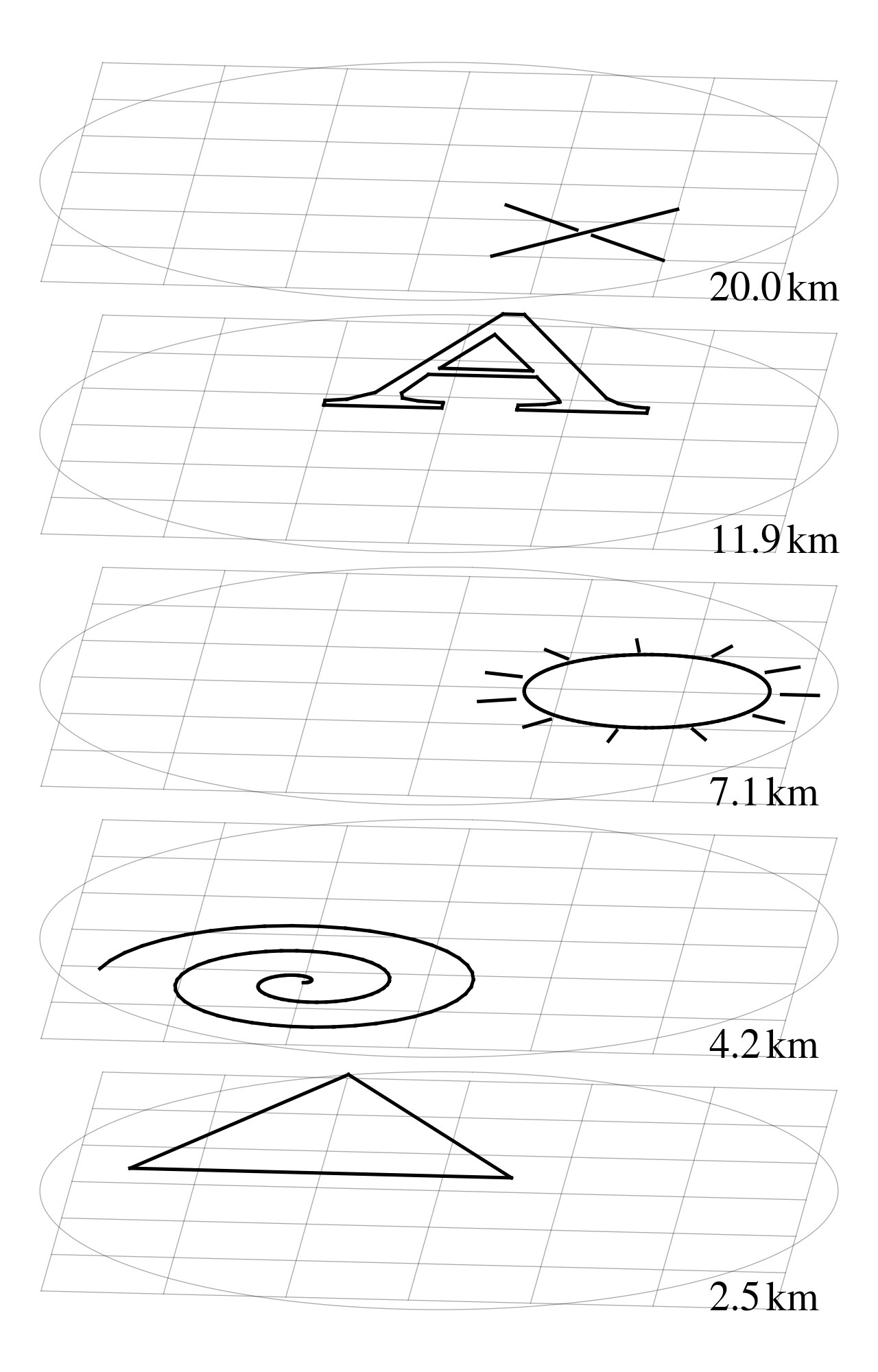
Figure 23: A phantom source in the atmosphere with five unique light emitting structures in five different depths. Grid has a spacing of $1^{\circ}$. Ring indicates the instrument’s field-of-view with a half-angle of $3.25^{\circ}$.

Telescope P-1

Figure 24: Observing the phantom source shown in Fig. 23 with the P-1 Cherenkov telescope. In the left column P-1’s state is (mirror: good, camera: good), while in the right column its state is (mirror: deformed, camera: misaligned).

Portal Plenoscope (P-61)

Figure 25: Observing the phantom source shown in Fig. 23 with the Portal Cherenkov plenoscope (P-61). In the left column Portal’s state is (mirror: good, camera: good), while in the right column its state is (mirror: deformed, camera: misaligned). See Fig. 24 for color bar.

10 Further Potential

10.1 Widening the Field-of-View

Sec. 6 demonstrates plenoptic’s potential to widen the field-of-view of imaging Cherenkov instruments. Already with Portal, which is not meant to push the boundaries of larger field-of-views, we find a comfortable 6.5 ^∘ of exceptional flat field-of-view. First simulations indicate the potential for a wide field-of-view, single mirror, all spherical surfaces plenoscope. We propose a design similar to Portal but with the screen of the light-field camera being curved to make its eyes point towards the center of the mirror. A field-of-view being significantly larger than 10^∘ seems reasonable.

10.2 Detecting Gamma Rays with Energies $>25$ GeV

For the detection of cosmic gamma rays with energies above $25$ GeV, arrays of Cherenkov telescopes are great. But plenoptics can improve Cherenkov telescopes, even existing ones, to profit from reduced aberrations, wider field-of-views, and more cost effective optics with only single mirrors and solely spherical surfaces. Arrays of Cherenkov telescopes do not need all of plenoptic’s features to profit. On telescopes with mirrors $<20\,$m there is not much depth to be perceived anyhow and arrays of such telescopes can combine their images after the fact to perceive depth. Also mirrors $<10\,$m will probably not profit too much from plenoptic’s adaptive compensation of deformations and misalignments. But to compensate aberrations one can build a simplified light-field camera where the imaging matrix $U(g)$ from Sec. 4.1 is fix and implemented into the analog summation of the photosensors. This way one only needs one analog-to-digital converter for each pixel in the final image. Such simplified light-field cameras might be a worthy upgrade for Cherenkov telescopes to reduce aberrations, widen the field-of-view, and potentially improve the directional reconstruction of the cosmic gamma rays.

10.3 Pushing the Stellar Intensity Interferometer

Beside observing the sky of gamma rays, the Portal Cherenkov plenoscope might at the same time image bright stars with angular resolutions approaching $\lambda/D=500\,$nm$/71\,$m$\,\approx 2\times 10^{-3}$ arc-seconds. Its plenoptic perception offers a unique opportunity for a stellar intensity interferometer. A stellar intensity interferometer needs ample bandwidths to correlate the signals of photosensors observing optical beams with same directions ($c_{x}$, $c_{y}$) but different impacts ($x$, $y$). Currently, in arrays of Cherenkov telescopes the beams to be correlated are scattered throughout the entire array and need adjustable delays in time in order to compensate the elongation or shortening of optical paths for different pointings. Therefore interferometers proposed for arrays of Cherenkov telescopes (Dravins et al., 2012) are held back by the limited bandwidth that can leave the individual telescope, effectively limiting either their field-of-view or exposure time. Now, the plenoscope on the other hand might continuously run an intensity interferometer across its entire field-of-view because here the beams to be correlated have their photosensors physically close to each other, inside the same housing, and do not need adjustable delays in time.

10.4 Perceiving Depth in Showers and Limits of the Atmospheric Cherenkov Method

After Portal has triggered, one can extract the Cherenkov photons from the pool of random photons coming from the night sky by means of clustering. Simulations indicate that the extracted Cherenkov-light field has a size of $\approx$100 photons for gamma rays with energies in the regime of $1\,$GeV to $2\,$GeV. With such sizes, the perception of depth becomes feasible. Eventually, the perception of depth is based on the statistics of multiple photons, as the individual photon does not have an observable which correlates to the depth of its emission. As images are a good start to discuss the statistics of multiple photons, one can project the recorded Cherenkov-light field onto many (several 1000) images, each with its focus set to a different depth $g$ in a range from e.g. 2.5 km to 25 km. In this stack of images, one finds a prominent cluster of Cherenkov light which grows and shrinks in solid angle when the stack of images is traversed along its dimension in depth. Also, the Cherenkov cluster deforms and slightly moves in the images when the stack is traversed along its dimension in depth.

First, one can find the depth along the stack of refocused images that minimizes the Cherenkov cluster’s spread in solid angle, compare Fig. 13. We find that this depth correlates with the depth where the shower has its maximum.

Second, one can characterize how quickly the Cherenkov cluster grows and shrinks in solid angle when the stack is traversed along its dimension in depth. If the Cherenkov cluster’s solid angle changes quickly with depth, the observed region where light was emitted is probably narrow in depth. On the other hand, if the Cherenkov cluster’s solid angle changes slowly with depth, the observed region where light was emitted is probably extended in depth.

Third, one can investigate how the Cherenkov cluster’s most dense region moves in the images when the stack of images is traversed along its dimension in depth. This hints to the orientation of the shower’s trajectory relative to the aperture’s principal plane and can potentially participate in the reconstruction of the cosmic gamma ray’s direction.

The Cherenkov cluster discussed here is less predictable than the Cherenkov ellipse which Hillas (1985) discusses based on simulations of gamma rays with energies in the regime of $1\,$TeV. Gamma rays with energies as low as 1 GeV, often induce showers which create no more than 10 light emitting particles. Here, fluctuations in the shower’s development have a noticeable effect on the statistics of the shower’s Cherenkov pool. Probably, these noticeable fluctuations will become the main challenge, and at some point the limit, of any atmospheric Cherenkov instrument which aims to observe cosmic gamma rays with energies as low as $1\,$GeV.

11 Outlook

We are looking forward to compile a series of papers discussing the all new Cherenkov plenoscope. This part discusses the optics. In the following parts we will evaluate the route towards an explorer for the timing in the sky of gamma rays which is based on the Portal Cherenkov plenoscope shown here. We are aiming for an energetic threshold of one giga electronvolt for cosmic gamma rays. We will evaluate Portal’s response functions, discuss the background from cosmic rays, and evaluate Portal’s performance to explore sudden cosmic events in the rapid sky of gamma rays.

12 Conclusion

The Cherenkov plenoscope has the potential to push the atmospheric Cherenkov method beyond the limits of the Cherenkov telescope. The concept of modeling beams of light and computing images after the fact has a great potential to widen the field-of-view, to compensate deformations in the mirror, to compensate misalignments of the camera, and to effectively overcome astronomy’s arch nemesis: Aberrations. By significantly reducing the demand for structural rigidity, the plenoscope has the potential to be built larger and more cost effective. By completely overcoming the telescope’s narrow depth-of-field and turning it into the perception of depth the plenoscope has the potential to be large enough to significantly lower the energetic threshold for cosmic gamma rays. As the Cherenkov plenoscope can have all these advantages at the same time, we might have the opportunity to implement the long anticipated and physically motivated vision(Aharonian, 2005) of a gamma ray timing explorer.

Appendix

App. A Calculating Image Rays

For the image ray’s direction $\vec{\delta}$ one first calculates the point

$$\vec{b} = f\left(-\frac{c_{x}}{\sqrt{1-c_{x}^{2}-c_{y}^{2}}},\,\,-\frac{c_{y}}{\sqrt{1-c_{x}^{2}-c_{y}^{2}}},\,\,1\right)^{T}$$ (18)

where the image ray intersects with the plane in focal-length $f$ according to the thin lens, and second subtracts the support from this point

$$\vec{\delta} = \frac{\vec{b}-\vec{s}}{|\vec{b}-\vec{s}|}.$$ (19)

Because Eq. 18 has no dependency of the optical path’s support $\vec{s}$ on the aperture, this image is free of aberrations.

App. B Calculating the Imaging Matrix

One calculates the elements $u_{n,\,k}(g)$ using the $k$-th image ray, and the $n$-th pixel’s position on a virtual screen which focuses on depth $g$. First, one calculates the distance of the image

$$b = \frac{1}{\frac{1}{f}-\frac{1}{g}},$$ (20)

based on one’s desired depth and puts the virtual screen right into this distance

$$d = b$$ (21)

to make it focus on $g$, see Fig. 4. Second, one calculates how far

$$\chi_{g} = \frac{d}{(0,0,1)\cdot\vec{\delta}_{k}}$$ (22)

one has to travel along the image ray $\vec{\rho}(\chi)_{k}$ to intersect with the virtual screen. Third, one calculates the intersection

$$\vec{i}_{k,g} = \vec{\rho}(\chi_{g})_{k}$$ (23)

of the image ray and virtual screen. Fourth, one looks up the position

$$\vec{p}_{n} = \left(x_{n},\,y_{n},\,d\right)^{T}$$ (24)

of the area on the virtual screen that feeds into the $n$-th pixel. These arbitrarily shaped areas, which feed into pixels, are defined in advance and describe how the image is binned. In most cases, one would probably choose this binning to be a regular grid of squares or hexagons. Fifth, one computes the distance

$$o_{n,k,g} = |\vec{i}_{k,g}-\vec{p}_{n}|$$ (25)

between the pixel’s area $\vec{p}_{n}$ and the image beam’s intersection $\vec{i}_{k,g}$ in the virtual screen. Finally, one can set the matrix’s elements

$$u_{n,\,k}(g) = \left\{\begin{array}[]{ll}1&\text{if}\,\,o_{n,k,g}\leq r_{n}\\ 0&\text{else}\\ \end{array}\right.{}$$ (28)

by comparing the distance $o_{n,k,g}$ to a threshold $r_{n}$ which can be e.g. the radius of the area feeding into the $n$-th pixel.

App. C Characterizing an Optical Beam

This is a simple definition for the spread of a beam which uses the instrument’s light-field calibration to gather statistics. In the light-field calibration, the $k$-th beam $\mathcal{B}{}_{k}$ is represented by a list of $P_{k}$ optical paths, see Eq. 3, and Eq. 5. We define the beam’s spread in solid angle to be the solid angle of an elliptical cone. The two half-angles of this elliptical cone are the standard deviations of the directions of the optical paths rays. For simplicity, we directly estimate these standard deviations from the components ${c_{x}}_{k,p}$, and ${c_{y}}_{k,p}$ and thus neglect potential smaller radii along the distribution’s principal axes. We apply the same method to estimate the beam’s spread in area, see Eq. 29, and Eq. 30.

$$\Omega{}_{k}= (4\pi\,\text{std}{}([{c_{x}}_{k,1},\dots c_{x}{}_{k,P_{k}}])$$ (29)

$$\,\text{std}{}([{c_{y}}_{k,1},\dots c_{y}{}_{k,P_{k}}]))$$

$$A{}_{k}= (4\pi\,\text{std}{}([{x}_{k,1},\dots x_{k,P_{k}}])$$ (30)

$$\,\text{std}{}([{y}_{k,1},\dots y_{k,P_{k}}])$$

For a beam’s spread in time we just compute the standard deviation of its delays ${\tau}_{k,p}$

$$T{}_{k} = \text{std}{}([{\tau}_{k,1},\dots\tau_{k,P}]),$$ (31)

and for the beam’s efficiency we compute the median of its optical paths efficiencies

$$E{}_{k} = \text{median}{}([{\eta}_{k,1},\dots\eta_{k,P}]).$$ (32)

In Fig. 12 we show the beams efficiencies relative to the median of all the $K$ beams efficiencies to not be spoiled by the particular coefficient of reflection of the mirror.

App. D Estimating Limits for Misalignments on a Telescope

These limits are motivated by Eq. 2 which apparently defines a change in an image to be significant when a considerable fraction ($\approx$ 100%) of the light expected to be assigned to one pixel ends up being assigned to a different pixel.

Translating Parallel

Translating the camera’s screen parallel to the mirror’s optical axis in the range

$$\Delta_{\parallel} = d-d_{\pm}$$ (33)

will not significantly change the image of a telescope. The start and stop distances of the camera’s screen

$$d_{\pm} = \frac{1}{\frac{1}{f}-\frac{1}{g_{\pm}}}$$ (34)

are estimated using Eq. 1 and Eq. 2.

Translating Perpendicular

Translating the camera’s screen perpendicular to the mirror’s optical axis up to about half the extent of a photosensor

$$\Delta_{\perp} \approx p/2$$ (35)

will not significantly effect the image.

Rotating Parallel

Rotating the camera’s screen mostly translates its outer edge which is in radial distance

$$r_{\text{camera}} = f\tan{(\Theta/2)}$$ (36)

from its optical axis. Here $\Theta/2$ is the half-angle of the instrumented field-of-view. Thus to not effect the image, a parallel rotation of the camera’s screen

$$\Phi_{\parallel} \approx \frac{\Delta_{\perp}}{r_{\text{camera}}}$$ (37)

must not translate a screen’s photosensor perpendicular by more than $\Delta_{\perp}$.

Rotating Perpendicular

Similar, rotating the camera’s screen perpendicular to the mirror’s optical axis

$$\Phi_{\perp} = \frac{\Delta_{\parallel}}{r_{\text{camera}}}$$ (38)

must not translate a photosensor parallel by more than $\Delta_{\parallel}$.

Author Contributions

S.A.M. leads the investigations, proposed the Cherenkov plenoscope, writes, runs, and analyses the simulations, and writes this manuscript. S.D. investigates Portal’s cable-robot mount in his master thesis in civil engineering with A.E. and E.C. reviewing his findings. A.B. supported the early investigations, reviews the feasibility of the optics, and supported A.A.E. to evaluate plenoptic reconstructions of atmospheric showers in A.A.E.’s master thesis. A.A.E. helps formulating the mindset of a light-field calibration. W.H. supports the investigations now and provides critical reviews on optics, statistics and language. M.L.A. and D.N. helped with early estimates of the plenoscope’s performance with M.L.A. further helping to find collaborators and motivating S.A.M. to commit and go ‘all in’ on the quest for a ‘gamma ray timing explorer’.

Additional Information

Computer simulations are public on https://github.com/cherenkov-plenoscope. Correspondence and requests for materials should be addressed to S.A.M.

Competing Financial Interests

The authors declare no competing financial interests.

References

- Abbott et al. (2017) Abbott, B., Abbott, R., Abbott, T., Acernese, F., Ackley, K., et al., 2017. Gravitational waves and gamma-rays from a binary neutron star merger: GW170817 and GRB170817A. The Astrophysical Journal Letters 848, L13. doi:10.3847/2041-8213/aa920c.
- Abdo et al. (2009) Abdo, A., Ackermann, M., Ajello, M., Atwood, W., Axelsson, M., et al., 2009. A population of gamma-ray millisecond pulsars seen with the Fermi Large Area Telescope. Science .
- Acero et al. (2015) Acero, F., Ackermann, M., Ajello, M., Albert, A, W., Axelsson, M., et al., 2015. Fermi Large Area Telescope third source catalog. The Astrophysical Journal Supplement Series 218, 23.
- Ackermann et al. (2014) Ackermann, M., Ajello, M., Asano, K., Atwood, W., Axelsson, M., et al., 2014. Fermi-LAT observations of the gamma-ray burst GRB 130427A. Science 343, 42–47.
- Aharonian (2005) Aharonian, F., 2005. Next generation of IACT arrays: Scientific objectives versus energy domains, Towards a Network of Atmospheric Cherenkov Detectors VII, Palaiseau, France.
- Aharonian et al. (2001) Aharonian, F., Konopelko, A., Völk, H, J., Quintana, H., 2001. 5@5–A 5 GeV energy threshold array of imaging atmospheric Cherenkov telescopes at 5 km altitude. Astroparticle Physics 15, 335–356.
- Ahnen et al. (2016a) Ahnen, M., Baack, D., Balbo, M., Bergmann, M., Biland, A., et al., 2016a. Bokeh mirror alignment for Cherenkov telescopes. Astroparticle Physics 82, 1–9.
- Ahnen et al. (2016b) Ahnen, M., Baack, D., Balbo, M., Bergmann, M., Biland, A., et al., 2016b. Normalized and asynchronous mirror alignment for Cherenkov telescopes. Astroparticle Physics 82, 56–65.
- Ailu et al. (2008) Ailu, E., Anderhub, H., et al., 2008. Observation of pulsed gamma-rays above 25 GeV from the Crab pulsar with MAGIC. Science 322, 1221–1224.
- Albert et al. (2008) Albert, J., Aliu, E., Anderhub, H., et al., 2008. Very-High-Energy gamma rays from a distant quasar: How transparent is the universe? Science 320, 1752–1754.
- Aleksić et al. (2014) Aleksić, J., Ansoldi, S., Antonelli, L., Antoranz, P., Babic, A., et al., 2014. Black hole lightning due to particle acceleration at subhorizon scales. Science 346, 1080–1084.
- Arbet Engels (2017) Arbet Engels, A., 2017. Cosmic ray composition measurements via direct Cherenkov light with the Atmospheric Cherenkov Plenoscope. ETH Zurich, Research Collection Institute for Particlephysics and Astrophysics.
- Arqueros et al. (2003) Arqueros, F., Jiménez, A., Valverde, A., 2003. A novel procedure for the optical characterization of solar concentrators. Solar Energy 75, 135–142.
- Bergholm et al. (2002) Bergholm, F., Renlund, E., Karl, F., 2002. The Plenoscope Concept and Image Formation, in: Swedish Society for Automated Image Analysis Symposium (SSAB), Uppsala Universitet. Centre for Mathematical Sciences, Lund University. pp. 75–78.
- Bernlöhr et al. (2013) Bernlöhr, K., Barnacka, A., Becherini, Y., Bigas, O., Carmona, E., et al., 2013. Monte Carlo design studies for the Cherenkov Telescope Array. Astroparticle Physics 43, 171–188.
- Biland et al. (2007) Biland, A., Garczarczyk, M., Anderhub, H., Danielyan, V., Hakobyan, D., et al., 2007. The Active Mirror Control of the MAGIC Telescope, in: Proceedings of the 30th ICRC, pp. 1353–1356.
- Borkowski (1987) Borkowski, K., 1987. Near zenith tracking limits for altitude-azimuth telescopes. Acta astronomica 37, 79.
- Bulian et al. (1998) Bulian, N., Daum, A., Hermann, G., Hess, M., Hofmann, W., et al., 1998. Characteristics of the multi-telescope coincidence trigger of the HEGRA IACT system. Astroparticle Physics 8, 223–233.
- Cornils et al. (2005) Cornils, R., Bernlöhr, K., Heinzelmann, G., Hofmann, W., Panter, M., 2005. The optical system of the H.E.S.S.-II telescope, in: International Cosmic Ray Conference, p. 171.
- Daglas (2017) Daglas, S., 2017. Structural Optimization of a NextGeneration Gamma-Ray Telescope. ETH Zurich, Research Collection Dept. of Civil, Environmental and Geomatic Engineering.
- Davies and Cotton (1957) Davies, J., Cotton, E., 1957. Design of the quartermaster solar furnace. Solar Energy 1, 16–22.
- Dibowski et al. (2023) Dibowski, H., Willsch, C., Raeder, C., 2023. High-Flux Solar Furnace and Xenon High-Flux Solar Simulator Customer Information. Deutsches Zentrum fuer Luft- und Raumfahrt e.V. (DLR).
- Dickinson et al. (2018) Dickinson, H., Krennrich, F., Weinstein, A., Eisch, J., Byrum, K., et al., 2018. An image-based array trigger for imaging atmospheric Cherenkov telescope arrays. Nuclear Instruments and Methods in Physics Research Section A: Accelerators, Spectrometers, Detectors and Associated Equipment 891, 6–17. doi:doi.org/10.1016/j.nima.2018.02.048.
- Dravins et al. (2012) Dravins, D., LeBohec, S., Jensen, H., Nuñez, P., 2012. Stellar intensity interferometry: Prospects for sub- milliarcsecond optical imaging. New Astronomy Reviews 56, 143–167.
- Funk et al. (2004) Funk, S., Hermann, G., Hinton, J., Berge, D., Bernlöhr, K., et al., 2004. The trigger system of the H.E.S.S. telescope array. Astroparticle Physics 22, 285–296.
- Garcia et al. (2014) Garcia, J., Dazzi, F., Häfner, D., Herranz, D., López, M., et al., 2014. Status of the new Sum-Trigger system for the MAGIC telescopes, 33th International Cosmic Ray Conference, Rio de Janeiro, Brazil.
- Hanrahan and Ng (2006) Hanrahan, P., Ng, R., 2006. Digital correction of lens aberrations in light field photography, in: International Optical Design Conference, Optical Society of America. p. WB2.
- Heck et al. (1998) Heck, D., Knapp, J., Capdevielle, J., Schatz, G., Thouw, T., et al., 1998. CORSIKA: A Monte Carlo Code to Simulate Extensive Air Showers. Forschungszentrum Karlsruhe 6019.
- Hillas (1985) Hillas, A., 1985. Cerenkov light images of EAS produced by primary gamma, in: International Cosmic Ray Conference.
- Hofmann (2001) Hofmann, W., 2001. How to focus a Cherenkov telescope. Journal of Physics G: Nuclear and Particle Physics 27, 933–939.
- Jung et al. (2005) Jung, I., Krawczynski, H., Buckley, J., Falcone, A., 2005. STAR a next generation Cherenkov telescope, in: Towards a Network of Atmospheric Cherenkov Detectors VII, pp. 463–6.
- Levoy et al. (2006) Levoy, M., Ng, R., Adams, A., Footer, M., Horowitz, M., 2006. Light Field Microscopy. ACM Transactions on Graphics (TOG), SIGGRAPH 25, 924–934.
- Lippmann (1908) Lippmann, G., 1908. Épreuves réversibles donnant la sensation du relief. J. Phys. Theor. Appl. 7 821-825 .
- López-Coto et al. (2016) López-Coto, R., Mazin, D., Paoletti, R., Bigas, O., Cortina, J., 2016. The Topo-trigger: a new concept of stereo trigger system for imaging atmospheric Cherenkov telescopes. Journal of Instrumentation 11, P04005.
- McCann et al. (2010) McCann, A., Hanna, D., Kildea, J., McCutcheon, M., 2010. A new mirror alignment system for the VERITAS telescopes. Astroparticle Physics 32, 325–329.
- Merklinger (1997) Merklinger, H., 1997. A technical view of bokeh. Photo Techniques 18.
- Miermeister et al. (2016) Miermeister, P., Lächele, M., Boss, R., Masone, C., Schenk, C., et al., 2016. The CableRobot Simulator: Large Scale Motion Platform Based on Cable Robot Technology, in: IEEE/RSJ International Conference on Intelligent Robots and Systems. IEEE/RSJ.
- Mirzoyan et al. (1996) Mirzoyan, R., Fomin, V., Stepanian, A., 1996. On the optical design of VHE gamma ray imaging Cherenkov telescopes. Nuclear Instruments and Methods in Physics Research Section A: Accelerators, Spectrometers, Detectors and Associated Equipment 373, 153–158.
- Mueller (2019) Mueller, S., 2019. Cherenkov-Plenoscope. ETH Zurich, doctoral thesis, No.:25833 arxiv.org, 1904.13368. doi:10.3929/ethz-b-000337911.
- de Naurois and Mazin (2015) de Naurois, M., Mazin, D., 2015. Ground-based detectors in Very-High-Energy gamma-ray astronomy. Comptes Rendus Physique 16, 610–627.
- Ng et al. (2005) Ng, R., Levoy, M., Brédif, M., Duval, G., Horowitz, M., et al., 2005. Light field photography with a hand-held plenoptic camera. Computer Science Technical Report CSTR 2.
- Okumura et al. (2016) Okumura, A., Noda, K., Rulten, C., 2016. ROBAST: Development of a ROOT-based ray-tracing library for cosmic-ray telescopes and its applications in the Cherenkov Telescope Array. Astroparticle Physics 76, 38–47.
- Pareschi et al. (2013) Pareschi, G., Armstrong, T., Baba, H., Bähr, J., Bonardi, A., et al., 2013. Status of the technologies for the production of the Cherenkov Telescope Array (CTA) mirrors, in: Optics for EUV, X-Ray, and Gamma-Ray Astronomy VI, International Society for Optics and Photonics. p. 886103.
- Perlin (1985) Perlin, K., 1985. An image synthesizer. ACM Siggraph Computer Graphics 19, 287–296.
- Schroedter et al. (2009) Schroedter, M., Anderson, J., Byrum, K., Drake, G., Duke, C., et al., 2009. A topological trigger system for imaging atmospheric-Cherenkov telescopes, 31st International Cosmic Ray Conference, Lodz, Poland.
- Tavani et al. (2011) Tavani, M., Bulgarelli, A., Vittorini, V., Pellizzoni, A., Striani, E., et al., 2011. Discovery of powerful gamma-ray flares from the Crab Nebula. Science 331, 736–739.
- Trichard et al. (2015) Trichard, C., Fiasson, A., Maurin, G., Lamanna, G., for the H.E.S.S. Collaboration, 2015. Enhanced H.E.S.S. II low energies performance thanks to the focus system, in: In Proceedings of the 34th International Cosmic Ray Conference (ICRC2015), The Hague, The Netherlands.
- Vassiliev and Fegan (2007) Vassiliev, V, V., Fegan, S, J., 2007. Schwarzschild-Couder two-mirror telescope for ground-based gamma-ray astronomy. 30-th ICRC .
- Weinstein et al. (2007) Weinstein, A., et al., 2007. The VERITAS trigger system, 30th International Cosmic Ray Conference, Merida, Mexico.
- Zinas and Daglas (2016) Zinas, G., Daglas, S., 2016. Design of a light weight supporting structure for next generation telescope, Semester Project Report Spring, Dept. Bau, Umwelt und Geomatik, ETH- Zurich.