A theory-independent bound saturated by quantum mechanics

Abstract

Tsirelson’s original inequality for the precession protocol, first introduced for the harmonic oscillator but applicable to all uniformly-precessing systems, serves as a monopartite test of quantumness. Given that the system is undergoing a uniform precession, the signs of the positions of a classical oscillator must satisfy that inequality, which is violated by certain quantum states. We consider this inequality for measurements with finitely many outcomes in a theory-independent manner. We derive a general bound which depends only on the minimum positive and negative values of the spectrum of the observable. Given any such two values, we construct a quantum observable that saturates this bound. A notable example is the angular momentum of a spin-$3/2$ particle. We also relate our findings to the recently-introduced notion of constrained conditional probabilities.

I Introduction

Given that the time evolution of the position of a harmonic oscillator is the same in both classical and quantum theory, it is remarkable that one can positively rule out classical theory using only position measurements at different times. The first protocol was invented by Tsirelson: under the assumption that an observable precesses uniformly in time, the average probability of it taking a positive value at three equally-spaced times is nontrivially bounded from above in classical theory; but this bound, or inequality, is violated by the quantum harmonic oscillator [1]. Since then, the precession protocol has been extended to spin angular momentum [2] and anharmonic dynamics [3], and also shown to be useful for witnessing entanglement in composite quantum systems [4, 5, 6].

However, we already know that the world does not behave according to classical theory. So, the question of whether a potential future theory behaves similarly to quantum theory under precession is at least equally pertinent. If it does not, this would provide a way to decide between different theories from observing their precession, like we can already do for classical and quantum theory.

At the same time, recent efforts in quantum foundations have aimed at identifying the features of quantum theory that make it unique and powerful for applications in computing or information theory. Such ideas [7, 8, 9] have been pursued in the framework of generalised probabilistic theories (GPTs) [10, 11]. In addition to aiding our understanding of quantum theory, these efforts may also lead to identifying new applications of quantum systems in the future.

In this work, we give first evidence that quantum systems perform optimally under uniform precession. Specifically, we derive a theory-independent bound for the original Tsirelson-type inequality, valid for all precessing discrete-variable systems. For this, we require that a theory has a notion of an observable that captures a measurement process, where we observe an outcome that occurs together with a transformation of the system under observation. Our Tsirelson-type inequality then applies under a few natural assumptions on the observables: that taking the mean value of a linear combination of observables is the same as the linear combination of the mean values, that the set of measurement outcomes is finite, and that the observables satisfy an algebraic equation that describes a uniform precession at the times of the measurements. In particular, all finite dimensional generalized probabilistic theories satisfy these assumptions, as do additional theories.

Given these assumptions, we show that the bound is saturated by quantum theory: in particular, the previously-studied case of the angular momentum of a spin-$3/2$ particle saturates the inequality.

In addition, we provide further insights into the differences between precession of classical and quantum systems: by analyzing the example of a clock, where the classical and quantum versions have the same spectrum; and by analyzing the probability spaces of the quantum observables defined here.

II The Original Inequality

Let us present the original inequality by Tsirelson in some generality with some relaxed assumptions. Consider two observables $A_{x}(t)$ and $A_{y}(t)$ that vary with time: these would be functions that output the values of $A_{x}$ or $A_{y}$ at time $t$ for the classical case, and operators in the Heisenberg picture for the quantum case. We say that $A_{x}$ precesses uniformly over the probing times $\{t_{0},t_{1},t_{2}\}$ if it satisfies

$$A_{x}(t_{k})=\cos(\frac{2\pi k}{3})A_{x}(t_{0})+\sin(\frac{2\pi k}{3})A_{y}(t_{0}).$$ (1)

In Tsirelson’s original formulation, $A_{x}$ was the position and $A_{y}$ the momentum of a harmonic oscillator with period $T$. Another natural example is provided by the $J_{x}$ and $J_{y}$ components of the angular momentum $\vec{J}$ of a system evolving under the Hamiltonian $H=-(2\pi/T)J_{z}$. In both these systems, the precession equation above holds at all times; here we relax the requirement and request it to be valid at least at times $\{t_{k}=kT/3\}_{k=0}^{2}$.

Under this assumption of uniform precession, each round of the protocol proceeds as follows:

1. Prepare the system in some state.

2. Choose at random which duration to wait among the possible $t_{k}\in\{t_{0},t_{1},t_{2}\}$.

3. Measure the corresponding $A_{x}(t_{k})$.

After many rounds, the score is calculated as

$$P_{3}:=\frac{1}{3}\sum_{k=0}^{2}\Big{\{}\underbrace{\Pr[A_{x}(t_{k})>0]+\frac{1}{2}\Pr[A_{x}(t_{k})=0]}_{=:\langle\operatorname{pos}[A_{x}(t_{k})]\rangle}\Big{\}}.$$ (2)

For classical theory, since the three points $\{A_{x}(t_{k})\}_{k=0}^{2}$ in $A_{x}$–$A_{y}$ space are equally distributed about a circle of radius $\sqrt{[A_{x}(t_{0})]^{2}+[A_{y}(t_{0})]^{2}}$ centered at the origin, they cannot be all positive or all negative. Therefore, the classical score is upper-bounded as $P_{3}\leq\mathbf{P}_{3}^{c}:=2/3$: this is Tsirelson’s original inequality, following the nomenclature by Plávala et al. [12]. Violation of this inequality was initially shown for the quantum harmonic oscillator (up to $P_{3}\gtrsim 0.709$) [1], and later for spin angular momentum (up to $P_{3}=3/4$) [2].

In this work, we analyze similar bounds for quantum and even more general theories, as will be introduced in the following section.

III Observables in General Theories

Our primary assumption in Eq. (1) is a statement on the observables $A_{x}$ and $A_{y}$. What observables are depends on the theory—these are real-valued random variables in classical theory and self-adjoint operators in quantum theory.

For general theories, let us consider what an observable means operationally. When an observable is measured on a system, we do so by applying some operation to the system (e.g. we might make it interact with a detector), after which we observe an outcome. Motivated by this, the notion of an observable in general theories would be a map that assigns to each outcome $a$ an operation $M_{a}$ on the system, $A:a\mapsto M_{a}$. We call the set of outcomes of an observable its spectrum $\lambda(A)$.

While the outcomes $a$ are taken to be real numbers, we leave open both the nature of the operations $M_{a}$, and how the outcome probabilities are obtained using $M_{a}$ and a description of the state of the system $s$. We do require the observables $A$ to satisfy two properties:

• Scalar multiplication of observables. If $A$ is an observable, the scalar multiplication of $A$ with a real number $c$ should result in another observable $cA$. This amounts to a change of scale, or of units. For a given state of a system $s$ and $c\neq 0$, if $a$ is a measurement outcome of $A$ with probability $\Pr(A=a|s)$, then $ca$ is a measurement outcome of $cA$ with the same probability, denoted now $\Pr(cA=ca|s)$. For $c=0$, we simply have that $0A=0$ is the observable that describes always observing the outcome $0$.

• Convex combination of observables. If $A_{1}$ and $A_{2}$ are observables, the convex combination $A=\lambda A_{1}+(1-\lambda)A_{2}$ for $0\leq\lambda\leq 1$ is another observable. This property is needed if the scenario, in which we measure one observable $A_{1}$ with probability $\lambda$, and otherwise another $A_{2}$, is itself to be described as “measuring an observable $A$”. Then the average for a given state $s$ must satisfy $\expectationvalue{A}_{s}=\lambda\expectationvalue{A_{1}}_{s}+(1-\lambda)\expectationvalue{A_{2}}_{s}$. Taken together with the previous property, it also implies that scaling the outcomes of an observable by $\lambda^{-1}$ with $\lambda\in(0,1)$, and then performing the observable with probability $\lambda$, results in the same observable.

These properties arguably should hold for any physical theory, insofar as they describe our operations rather than properties of nature. At any rate, they are satisfied by all finite-dimensional GPTs [7, 8, 9, 10, 11], as proved in Appendix A; and thus in particular by classical and quantum theories. They may also hold in theories that do not obey the usual restrictions imposed on GPTs: for instance, in Appendix B we construct a generalized theory with a toroidal effect space that is nonconvex and hence does not satisfy the axioms of generalized probabilistic theories, but where the above two properties still hold.

These two properties imply the linearity of the expectation value

$$\expectationvalue{c_{1}A_{1}+c_{2}A_{2}}_{s}=c_{1}\expectationvalue{A_{1}}_{s}+c_{2}\expectationvalue{A_{2}}_{s}$$ (3)

for any two observables $A_{1}$, $A_{2}$ and real scalars $c_{1}$, $c_{2}$ (while the prescription on how the individual outcomes are defined may vary with the theory). Then, Eq. (1) implies immediately that

$$\expectationvalue{A_{x}(t_{k})}_{s}=\cos(\frac{2\pi k}{3})\expectationvalue{A_{x}(t_{0})}_{s}+\sin(\frac{2\pi k}{3})\expectationvalue{A_{y}(t_{0})}_{s}.$$ (4)

From the sum of the roots of unity $\sum_{k=0}^{2}e^{i2\pi k/3}=0$, this further implies that

$$\frac{1}{3}\sum_{k=0}^{2}\expectationvalue{A_{x}(t_{k})}_{s}=0.$$ (5)

IV Discrete Variable Systems

In this work, we consider systems where the spectrum of the measured observable is discrete and finite. We further define the spectrum in a purely operational manner: the spectrum $\lambda(A_{x})$ of $A_{x}$ is simply all possible measurement outcomes of $A_{x}$ over all times $\{t_{k}\}_{k=0}^{2}$, written as

$$\lambda(A_{x})=\{-a_{-d_{-}},\dots,-a_{-2},-a_{-1},\underbrace{0}_{\text{(might not be included)}},a_{+1},\dots,a_{+d_{+}}\},$$ (6)

with $-a_{-d_{-}}<\dots<-a_{-2}<-a_{-1}<0<a_{+1}<a_{+2}<\dots<a_{+d_{+}}$. The value $0$ might not be included in the spectrum (e.g. in the quantum description of the angular momentum of half-integer spins), and the spectrum could also be nonnegative ($d_{-}=0$) or nonpositive ($d_{+}=0$). Futhermore, note that while the definition of the spectrum in general theories is slightly more general (allowing for POVMs), for a quantum observable specified by an operator, the spectrum corresponds exactly to its mathematical spectrum.

An example of a discrete variable system in classical theory could be the projection of the hand of an analog clock onto one of its diameters. The possible measurement outcomes are $\{l\cos(s\pi/30)\}_{s=0}^{30}$, where $l$ is the length of the hand, and we use the familiar convention of dividing the circle into 60 units (minutes or seconds). Eq. (1) is then satisfied for the horizontal diameter $A_{x}$ and vertical diameter $A_{y}$, with the three probing times $t_{k}=20k$. Quantum examples abound, as the spectrum of quantum observables are discrete for all uniformly-precessing finite-dimensional systems.

V Theory-independent Bound

For a given initial state of the system $s$, we shall denote the probability of measuring $A_{x}(t_{k})$ and observing $\pm a_{\pm j}\in\lambda(A_{x})$ as $p_{\pm j}(t_{k}):=\Pr[A_{x}(t_{k})=\pm a_{\pm j}|s]$, henceforth dropping any reference to $s$.

With this notation, Eq. (2) reads

$$P_{3}=\frac{1}{3}\sum_{k=0}^{2}\sum_{j=1}^{d_{+}}p_{+j}(t_{k})+\frac{1}{6}\sum_{k=0}^{2}p_{0}(t_{k}).$$ (7)

For the special case when $\lambda(A_{x})$ is nonnegative, we have from Eq. (5) that

$$\sum_{k=0}^{2}\expectationvalue{A_{x}(t_{k})}=0=\sum_{k=0}^{2}\sum_{j=1}^{d_{+}}a_{+j}p_{+j}(t_{k}).$$ (8)

Since $a_{+j}>0$ for all $j$, the only possibility is $p_{+j}(t_{k})=0$ for all $j$ and $k$. If $0\in\lambda(A_{x})$, this implies that $p_{0}(t_{k})=1$ for all $k$ and hence $P_{3}=1/2$. If $0\notin\lambda(A_{x})$, Eq. (8) cannot be satisfied and hence $A_{x}$ is not uniformly-precessing. An analogous proof shows that $P_{3}=1/2$ when $\lambda(A_{x})$ is nonpositive and $0\in\lambda(A_{x})$.

We henceforth need only consider the cases where the spectrum contains both positive and negative values, such that $d_{\pm}\geq 1$.

Starting from

$$\expectationvalue{A_{x}(t)}=\sum_{j=1}^{d_{+}}a_{+j}p_{+j}(t)-\sum_{j^{\prime}=1}^{d_{-}}a_{-j^{\prime}}p_{-j^{\prime}}(t)=\sum_{j=1}^{d_{+}}a_{+j}p_{+j}(t)-\sum_{j^{\prime}=1}^{d_{-}-1}a_{-j^{\prime}}p_{-j^{\prime}}(t)-a_{-d_{-}}p_{-d_{-}},$$ (9)

and using the normalization condition $\sum_{j=1}^{d_{+}}p_{+j}(t)+\sum_{j^{\prime}=1}^{d_{-}}p_{-j^{\prime}}(t)+p_{0}(t)=1$, we have

$$\expectationvalue{A_{x}(t)} =\sum_{j=1}^{d_{+}}a_{+j}p_{+j}(t)-\sum_{j^{\prime}=1}^{d_{-}-1}a_{-j^{\prime}}p_{-j^{\prime}}(t)-a_{-d_{-}}\bqty{1-p_{0}(t)-\sum_{j=1}^{d_{+}}p_{+j}(t)-\sum_{j^{\prime}=1}^{d_{-}-1}p_{-j^{\prime}}(t)}$$ (10)

$$=\sum_{j=1}^{d_{+}}\pqty{a_{+j}+a_{-d_{-}}}p_{+j}(t)-a_{-d_{-}}+a_{-d_{-}}p_{0}(t)+\sum_{j^{\prime}=1}^{d_{-}-1}\pqty{a_{-d_{-}}-a_{-j^{\prime}}}p_{-j^{\prime}}(t).$$

Since $a_{-d_{-}}\geq a_{-j^{\prime}}$ for all $j^{\prime}$ and $p_{-j^{\prime}}(t)\geq 0$, we must have $\sum_{j^{\prime}=1}^{d_{-}-1}\pqty{a_{-d_{-}}-a_{-j^{\prime}}}p_{-j^{\prime}}(t)\geq 0$ for the last term, so

$$\begin{gathered}0\leq\expectationvalue{A_{x}(t)}-\bqty{\sum_{j=1}^{d_{+}}\pqty{a_{+j}+a_{-d_{-}}}p_{+j}(t)-a_{-d_{-}}+a_{-d_{-}}p_{0}(t)}\\ \implies\sum_{j=1}^{d_{+}}\pqty{a_{+j}+a_{-d_{-}}}p_{+j}(t)\leq\expectationvalue{A_{x}(t)}+a_{-d_{-}}-a_{-d_{-}}p_{0}(t).\end{gathered}$$ (11)

Therefore,

$$\expectationvalue{\operatorname{pos}[A_{x}(t)]}=\sum_{j=1}^{d_{+}}p_{+j}(t)+\frac{1}{2}p_{0}(t) \leq\sum_{j=1}^{d_{+}}\frac{a_{+j}+a_{-d_{-}}}{a_{+1}+a_{-d_{-}}}p_{+j}(t)+\frac{1}{2}p_{0}(t)$$ (12)

$$\leq\frac{\expectationvalue{A_{x}(t)}+a_{-d_{-}}-a_{-d_{-}}p_{0}(t)}{a_{+1}+a_{-d_{-}}}+\frac{1}{2}p_{0}(t)$$

$$=\frac{\expectationvalue{A_{x}(t)}}{a_{+1}+a_{-d_{-}}}+\frac{a_{-d_{-}}}{a_{+1}+a_{-d_{-}}}+\frac{a_{+1}-a_{-d_{-}}}{2(a_{-d_{-}}+a_{+1})}p_{0}(t).$$

If $a_{+1}<a_{-d_{-}}$, then the last term is negative and can be upper bounded by $0$. Similarly, the last term is zero when $0\notin\lambda(A_{x})$. Otherwise, $\frac{a_{+1}-a_{-d_{-}}}{2(a_{-d_{-}}+a_{+1})}p_{0}(t)\leq\frac{a_{+1}-a_{-d_{-}}}{2(a_{-d_{-}}+a_{+1})}$ from the requirement that $p_{0}(t)\leq 1$ is a probability. Then,

$$\expectationvalue{\operatorname{pos}[A_{x}(t)]} \leq\frac{\expectationvalue{A_{x}(t)}}{a_{+1}+a_{-d_{-}}}+\begin{cases}\frac{2a_{-d_{-}}}{2(a_{+1}+a_{-d_{-}})}&\text{if $a_{+1}<a_{-d_{-}}$ or $0\notin\lambda(A_{x})$}\\[6.45831pt] \frac{2a_{-d_{-}}+a_{+1}-a_{-d_{-}}}{2(a_{+1}+a_{-d_{-}})}&\text{otherwise}\end{cases}$$ (13)

$$=\frac{\expectationvalue{A_{x}(t)}}{a_{+1}+a_{-d_{-}}}+\begin{cases}(1+a_{+1}/a_{-d_{-}})^{-1}&\text{if $a_{+1}<a_{-d_{-}}$ or $0\notin\lambda(A_{x})$}\\ 1/2&\text{otherwise}\end{cases}$$

Finally, we have

$$P_{3}=\frac{1}{3}\sum_{k=0}^{2}\expectationvalue{\operatorname{pos}[A_{x}(t_{k})]} \leq\frac{1}{3(a_{+1}+a_{-d_{-}})}\overbrace{\sum_{k=0}^{2}\expectationvalue{A_{x}(t_{k})}}^{0\text{ from Eq.~{}\eqref{eq:means-precess-sum}}}+\overbrace{\frac{1}{3}\sum_{k=0}^{2}}^{1}\begin{cases}(1+a_{+1}/a_{-d_{-}})^{-1}&\text{if $a_{+1}<a_{-d_{-}}$ or $0\notin\lambda(A_{x})$}\\ 1/2&\text{otherwise}\end{cases}$$ (14)

$$=\begin{cases}(1+a_{+1}/a_{-d_{-}})^{-1}&\text{if $a_{+1}<a_{-d_{-}}$ or $0\notin\lambda(A_{x})$}\\ 1/2&\text{otherwise}\end{cases}$$

$$=:\mathbf{P}_{3}^{G}(a_{+1}/a_{-d_{-}}).$$

Therefore, the general bound depends solely on the ratio between the minimum positive and negative measurement outcomes, respectively $a_{+1}=\min\{a\in\lambda(A_{x}):a>0\}$ and $-a_{-d_{-}}=\min\{a\in\lambda(A_{x}):a<0\}$. Note that Eq. (14) nicely includes the special cases: if the spectrum is nonnegative (nonpositive), then $a_{-d_{-}}$ ($a_{+1}$) is undefined while we must also have $0\in\lambda(A_{x})$ for it to be uniformly-precessing, so $a_{+1}/a_{-d_{-}}\nless 1$ and $\mathbf{P}^{G}_{3}=1/2$ as previously found.

VI Saturation by Quantum Theory

We shall now prove by construction that the general bound is saturated by quantum theory: that is, for a given $a_{+1}$ and $a_{-d_{-}}$, it is always possible to construct a uniformly-precessing quantum observable that achieves $P_{3}=\mathbf{P}_{3}^{G}$.

Consider the four-level system

$$A_{x} :=(a_{-d_{-}}-a_{+1})\pqty{\outerproduct{1}{2}+\outerproduct{2}{1}}$$ (15)

$$\qquad{}+{}\sqrt{a_{+1}a_{-d_{-}}}\pqty{\outerproduct{0}{1}+\outerproduct{1}{0}+\outerproduct{2}{3}+\outerproduct{3}{2}},$$

$$A_{y} :=-i(a_{-d_{-}}-a_{+1})\pqty{\outerproduct{1}{2}-\outerproduct{2}{1}}$$

$$\qquad{}-{}i\sqrt{a_{+1}a_{-d_{-}}}\pqty{\outerproduct{0}{1}-\outerproduct{1}{0}+\outerproduct{2}{3}-\outerproduct{3}{2}},$$

where $a_{-d_{-}}>a_{+1}>0$. $A_{x}$ can be easily diagonalized using standard techniques to find that its spectrum is $\{-a_{-d_{-}},-a_{+1},a_{+1},a_{-d_{-}}\}$ with the eigenstates

$$\ket{\pm a_{-d_{-}}} \propto\sqrt{a_{+1}}\pqty{\ket{0}\pm\ket{3}}\pm\sqrt{a_{-d_{-}}}\pqty{\ket{1}\pm\ket{2}},$$ (16)

$$\ket{\pm a_{+1}} \propto\sqrt{a_{-d_{-}}}\pqty{\ket{0}\mp\ket{3}}\pm\sqrt{a_{-d_{-}}}\pqty{\ket{1}\mp\ket{2}}.$$

Under the Hamiltonian $H=\omega\sum_{n=0}^{3}n\outerproduct{n}{n}$, the observable $A_{x}$ evolves in time as

$$A_{x}(t)=e^{iHt}A_{x}e^{-iHt}=\cos(\omega t)A_{x}+\sin(\omega t)A_{y}.$$ (17)

By choosing the probing times to be $t_{k}=2\pi k/3\omega$, Eq. (1) is satisfied.

With these observables, Hamiltonian, and probing times, the state $\ket{\mathbf{P}_{3}}:=(\ket{0}-\ket{3})/\sqrt{2}$ achieves the score

$$P_{3} =\frac{1}{3}\sum_{k=0}^{2}\bra{\mathbf{P}_{3}}\operatorname{pos}[A_{x}(t_{k})]\ket{\mathbf{P}_{3}}$$ (18)

$$=\frac{1}{3}\sum_{k=0}^{2}\absolutevalue{\bra{a_{+1}}e^{-iHt_{k}}\ket{\mathbf{P}_{3}}}^{2}+\absolutevalue{\bra{a_{-d_{-}}}e^{-iHt_{k}}\ket{\mathbf{P}_{3}}}^{2}$$

$$=\frac{1}{1+a_{+1}/a_{-d_{-}}}=\mathbf{P}_{3}^{G}(a_{+1}/a_{-d_{-}}),$$

which saturates the general bound. Notice that $\mathbf{P}_{3}^{G}$ can be made arbitrarily close to $1$ by choosing $a_{-d_{-}}$ to be arbitrary large, but one cannot set $a_{+1}=0$ because by definition $a_{+1}$ is the smallest positive value of the spectrum: said differently, setting it to be $0$ amounts to saying that the spectrum is $\lambda(A_{x})=\{-a_{-d_{-}},0,a_{-d_{-}}\}$, which implies $\min\{a\in\lambda(A_{x}):a>0\}=a_{-d_{-}}$, whereupon $\mathbf{P}_{3}^{G}=1/2$.

A special case is obtained when we set $a_{+1}/a_{-d_{-}}=3$, in which case $A_{x}\propto J_{x}$ and $A_{y}\propto J_{y}$ for $j=3/2$. This also shows that the previously found quantum violation of $P_{3}=3/4$ by the angular momentum operators of a spin-$3/2$ particle [2] is the maximum possible violation that can be found in any general theory that shares its spectrum.

That said, a direct comparison is difficult between classical and quantum theory for the spin-$3/2$ particle, as there are no uniformly precessing classical observables with the same spectrum. We can revisit the analog clock for an example where both the classical and quantum variables share the same spectrum. For some $N$ that is a positive multiple of $6$, consider

$$C_{x} :=\frac{l}{2}\pqty{S_{N}^{\dagger}+S_{N}}\oplus A_{x},$$ (19)

$$C_{y} :=\frac{l}{2i}\pqty{S_{N}^{\dagger}-S_{N}}\oplus A_{y};$$

where $S_{N}:=\outerproduct{0}{N-1}+\sum_{n=0}^{N-2}\outerproduct{n+1}{n}$ is the shift operator, and $A_{x}$, $A_{y}$ are as defined in Eq. (15) with $a_{-d_{-}}$ and $a_{+1}$ to be chosen.

The spectrum of the shift operator is well-known [13], from which $l(S_{N}^{\dagger}+S_{N})/2$ can be found to have eigenvalues $\{l\cos(2\pi n/N)\}_{n=0}^{N-1}$ with eigenstates

$$\ket{l\cos(2\pi n/N)}\propto\sum_{n^{\prime}=0}^{N-1}e^{i2\pi nn^{\prime}/N}\ket{n^{\prime}}.$$ (20)

As such, by choosing $a_{-d_{-}}$ and $a_{+1}$ of $A_{x}$ to be

$$a_{-d_{-}} =-\min\{l\cos(2\pi n/N)\}_{n=0}^{N-1}=l,$$ (21)

$$a_{+1} =\min\{l\cos(2\pi n/N):l\cos(2\pi n/N)>0\}_{n=0}^{N-1}$$

$$=l\cos[2\pi(\lceil N/4\rceil-1)/N],$$

we have $\lambda(C_{x})=\{l\cos(2\pi n/N)\}_{n=0}^{N-1}$, with the extremal values of $\lambda(C_{x})$ corresponding exactly to those of $A_{x}$. This spectrum is shared by a classical analog clock with $N$ divisions, with $N=60$ being a standard clock face divided into minutes or seconds.

It can also be verified that Eq. (1) is satisfied by $C_{x}(t_{k}):=U^{{\dagger}k}C_{x}U^{k}$ where $U:=\exp(-i\frac{2\pi}{3}\sum_{n}n\outerproduct{n}{n})$, so $C_{x}$ is uniformly-precessing. Meanwhile, the inclusion of $A_{x}$ from Eq. (15) in Eq. (19) ensures that $C_{x}$ achieves the score $\mathbf{P}_{3}^{G}$. For the standard clock face, this gives $\mathbf{P}_{3}^{G}=(1+\cos(7\pi/15))^{-1}\approx 0.905$. This is hence an example of a quantum observable with a spectrum shared by a classical observable that also saturates the general bound.

VII Probability Spaces of Precessing Variables

Our findings have some ramifications on the recently introduced study of constrained conditional probability spaces [12]. There, the authors considered the probability space spanned by all possible tuples $(\langle\operatorname{pos}[A_{x}(t_{k})]\rangle)_{k=0}^{2}$ achievable in classical theory. The full, unrestricted probability space $\mathcal{P}$, which is only constrained by ${0\leq\langle\operatorname{pos}[A_{x}(t_{k})]\rangle\leq 1}\ \forall k$, is given by the cube

$$\mathcal{P}:=\operatorname{Conv}\!\bqty{\Bqty{(s_{0},s_{1},s_{2}):s_{l}\in\{0,1\}}},$$ (22)

where $\operatorname{Conv}(\mathcal{S})$ is the convex hull of $\mathcal{S}$. It was shown that the constraint that $A_{x}$ should change signs at least once, which comes from the requirement that it precesses, results in a strictly-smaller polytope $\mathcal{C}\subsetneq\mathcal{P}$ for classical observables, where

$$\mathcal{C} :=\operatorname{Conv}\!\big{[}\Bqty{(s_{0},s_{1},s_{2})\!:\!s_{l}\!\in\!\{0,1\}}\setminus{}\{(0,0,0),(1,1,1)\}\big{]}.$$ (23)

Tsirelson’s original inequality then arises from the nontrivial facet $\operatorname{Conv}\!\big{[}\{(0,1,1),(1,0,1),(1,1,0)\}\big{]}$.

Figure 1: (a) Probability space $\mathcal{Q}^{(j=3/2)}_{J_{x}}$ for the outcomes of performing the precession protocol on $J_{x}$ of a spin $j=3/2$ particle. The translucent blue polytope, with its extreme points in red, is the constrained probability space $\mathcal{C}$ that marks out the possible tuples $(\langle\operatorname{pos}[A_{x}(t_{k})]\rangle)_{k=0}^{2}$ achievable by a classical uniformly-precessing observable. The triangular nontrivial facet $\operatorname{Conv}\!\big{[}\{(0,1,1),(1,0,1),(1,1,0)\}\big{]}$ defines the original Tisrelson inequality $P_{3}=\sum_{k=0}^{2}\langle\operatorname{pos}[A_{x}(t_{k})]\rangle/3>2/3$. The surface is coloured according to its distance from the closest nontrivial facet. Both the classical and quantum sets are symmetric upon reflection about the $P_{3}=1/2$ plane. (b) A linecut of $\mathcal{Q}^{(j=3/2)}_{J_{x}}$ from $(1/2,1/2,1)$ to $(1,1,0)$. The classical and general bounds are the dashed line labelled $\mathbf{P}_{3}^{c}$ and $\mathbf{P}_{3}^{G}$ respectively.

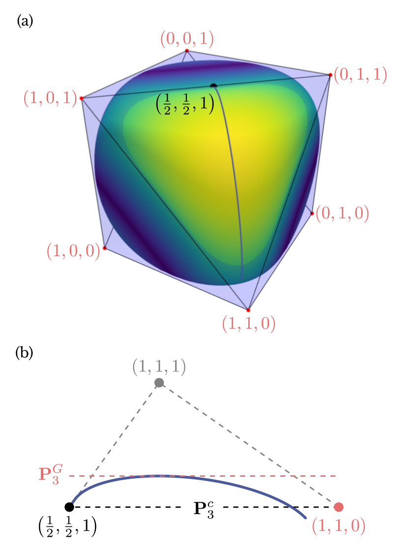
The probability space of a given quantum observable $A_{x}(t_{k})$ can be found using a semidefinite program, whose details are given in Appendix C. The case of $J_{x}(t_{k})$ for the spin-$3/2$ particle is shown in Fig. 1. While there is no classical analog of an observable with the same spectrum as a spin-$3/2$ particle, we have nonetheless superimposed the classical polytope that must be satisfied by every uniformly precessing classical observable. A substantial volume of the spin-$3/2$ probability space $\mathcal{Q}^{(j=3/2)}_{J_{x}}$ extrudes out of the nontrivial facet, demonstrating the violation of the classical bound. Meanwhile, the neighborhood of the extremal points of the classical polytope cannot be reached with the quantum system under study.

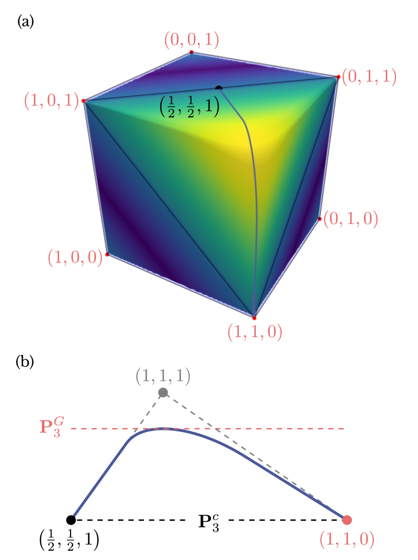
We can also consider the probability space $\mathcal{Q}_{\text{clock}}^{(N)}$ for the clock observable in Eq. (19) with $N=60$. The tuples $(\bra{n}\operatorname{pos}[C_{x}(t_{k})]\ket{n})_{k=0}^{2}$ for $0\leq n\leq N-1$ form the extreme vertices of $\mathcal{C}$, and therefore their convex combinations replicate the entire classical set. Meanwhile, there are also many points outside the nontrivial facet of $\mathcal{C}$. As such, $\mathcal{C}\subsetneq\mathcal{Q}_{\text{clock}}^{(N=60)}\subsetneq\mathcal{P}$, as can be seen in Fig. 2.

In general, for any $N$, we have $\overline{\mathcal{Q}}^{(N)}_{\text{clock}}\subseteq\mathcal{Q}^{(N)}_{\text{clock}}$, where

$$\overline{\mathcal{Q}}^{(N)}_{\text{clock}}:=\operatorname{Conv}\!\Big{[}\mathcal{C} {}\cup{}\Bqty{\pqty{\mathbf{P}_{3}^{G},\mathbf{P}_{3}^{G},\mathbf{P}_{3}^{G}}}$$ (24)

$${}\cup{}\Bqty{\pqty{1-\mathbf{P}_{3}^{G},1-\mathbf{P}_{3}^{G},1-\mathbf{P}_{3}^{G}}}\Big{]},$$

since $\ket{\mathbf{P}_{3}}$ from Eq. (18) and $e^{-i\pi\sum_{n}\outerproduct{n}{n}}\ket{\mathbf{P}_{3}}$ can be verified to form the vertices $(\mathbf{P}_{3}^{G})_{k=0}^{2}$ and $(1-\mathbf{P}_{3}^{G})_{k=0}^{2}$ respectively.

Furthermore, as $\mathbf{P}_{3}^{G}=(1+{\cos}[2\pi(\lceil N/4\rceil-1)/N])^{-1}\to 1$ as $N\to\infty$, we also have $\overline{\mathcal{Q}}^{(N)}_{\text{clock}}\to\mathcal{P}$, which in turn implies that $\overline{\mathcal{Q}}^{(N)}_{\text{clock}}\subseteq\mathcal{Q}^{(N)}_{\text{clock}}\to\mathcal{P}$. This shows that the quantum set can reach arbitrarily close to the full probability space with an observable that has a finite but arbitrarily large number of measurement outcomes.

Figure 2: Probability space $\mathcal{Q}_{\text{clock}}^{(N=60)}$ for a quantum observable with the same spectrum as the horizontal and vertical position of the second hand of an analogue clock. The quantum observable saturates the general bound, and the quantum set not only contains the classical set, but also almost entirely fills up the full probability space.

VIII Difference between the theory-independent bound and actual precession

Notice that the theory-independent bound on $P_{3}$ is derived only from the form of the observables, without taking into account the requirement that the precession is caused by a time evolution within the theory. Hence, it might seem surprising at first that uniformly-precessing systems in quantum theory satisfy the upper bound.

Other theories, despite satisfying the assumptions from Section III, do not precess in this sense. To illustrate this, let us consider the example of boxworld, also known as generalized non-signalling theory [11]. If we consider a single system in this theory, a system characterized by $d$ 2-outcome measurements can be represented as a $d$-dimensional hypercube. Reversible transformations on this system are then a subgroup of the symmetry group of the state space and thus in this example discrete [14, 15]. This means that we cannot define precession with a continuous parameter $t$ in this case.

One could instead aim at constructing precessing systems with discrete rotations. While there are still rotations of order $3$ in the case of a (hyper-)cube, this can not be straightforwardly generalized to boxworld systems where measurements have more than two outcomes, which we would like to use to construct precessing systems. This can be seen most easily as the number of extremal states of a single system is $(\#\text{ outcomes})^{\#\text{ inputs}}$, which generally does not coincide with the number of extremal vertices of a hypercube. Because of this, we were not able to even build interesting precessing systems in this theory.

On the other hand, there are also theories that have been built as adaptations of quantum theory. These include quantum theory over real Hilbert spaces and Grassmannian systems [16, 17], which also saturate our bound (see Appendix D). We leave for future works to assess whether all systems that accommodate uniform precession and saturate our theory-independent bound are as closely related to quantum theory as these. In this sense, this work falls short of providing the first example of a self-test of quantum theory [8, 9]: the latter remains a conjecture.

IX Conclusion

In this work, a theory-independent bound was derived for the original Tsirelson-type inequality of the precession protocol applied to discrete variable systems. We showed that this bound depends on the spectrum of the measured observables, and that no general theory with finite measurement outcomes can outperform quantum mechanics. We have also shown that the previously-studied spin-$3/2$ case optimally violates the precession protocol. Finally, we related our work to the study of constrained conditional probability spaces, and demonstrated that the quantum set reaches arbitrarily closely to the full unconstrained probability space.

Other relevant studies with a similar flavor include work on spin-bounded rotation boxes [18, 19], where the authors considered general systems transforming under an $\operatorname{SO}(2)$ rotation. Our fundamental assumptions differ, as their assumption is on the measurement probabilities (that they are given by a Fourier series with a bounded number of terms), while ours is on the observables (that they precess uniformly). A future avenue of research could be to borrow ideas from their approach. Strictly speaking, we have only imposed a $\mathbb{Z}_{3}$ symmetry on the $A_{x}$: what if we imposed an $\operatorname{SO}(2)$ symmetry in the same vein as the authors, or perhaps even $\operatorname{SO}(3)$? The latter restriction would impose that the measured observables $A_{x}$ and $A_{y}$ should be components of a three-dimensional vector $(A_{x},A_{y},A_{z})$. The general bound we derived here is not saturated by any angular momentum of spin $j>3/2$; nor did we find any other example of vectors in quantum theory that saturated the general bound. It remains to be seen if these imposed symmetries would tighten the bound for vectorial quantities.

It would also be interesting to extend this result to the continuous variable case. However, the study of continuous-variable generalized theories [20] is still in its infancy, even for GPTs: we were unable to tackle this problem with the existing tools, and thus leave this for the future when the appropriate tools have been developed.

We have also only focused on the Tsirelson-type inequality that was introduced in the original paper, which involves probing the system at $3$ different times. Another possible extension of this work would be to derive similar theory-independent bounds for the Tsirelson-type inequalities that were introduced later, where the system is probed at $K>3$ different times for $K$ odd.

Appendix A Generalized Probabilistic Theories

Generalized probabilistic theories (GPTs) were introduced to study physical theories operationally, in terms of sate preparations, evolutions and measurements [10, 11]; see [21] for a recent review. Both classical and quantum theories are examples of GPTs, although the landscape of GPTs is much richer, including theories like boxworld [11] and generalized qubits [22].

In GPTs, possible states live in a state space $\mathcal{S}\subset V$, a convex compact set in a real vector space $V$. The effects of that theory form a convex subset $\mathcal{E}\subseteq\mathcal{E}_{\rm max}:=\{e\in V^{*}:0\leq e(s)\leq 1\;\forall s\in\mathcal{S}\}$. The set $\mathcal{E}$ further has to contain the unique effect $u\in\mathcal{E}$ that satisfies $\forall s\in\mathcal{S}:u(s)=1$ and the zero effect $\forall s\in\mathcal{S}:\mathbf{0}(s)=0$. Any measurement is made up of a set of effects $\{e^{x}\}_{x\in X}\subseteq\mathcal{E}$ such that $\sum_{x\in X}e^{x}=u$, where $X\subset\mathbb{R}$ is the set of measurement outcomes. In this work we only consider measurements with a finite number of outcomes. The probability of obtaining the outcome $x$ given the state $s$ is given by $\Pr(x|s)=e^{x}(s)$.

Any such measurement can define an observable [23, 15] in the sense of a map $A:x\mapsto e^{x}$ where the expectation value on any state $s\in\mathcal{S}$ satisfies

$$\left\langle A\right\rangle_{s}=\sum_{x\in X}x\Pr(x|s)=\sum_{x\in X}xe^{x}(s).$$ (25)

We will call the set of outcomes the spectrum of A, $\lambda(A)=X$. Notice further that each measurement outcome $x$ can be changed independently to some $f(x)$, for example, using some classical post-processing. This leads to a new observable $f(A):f(x)\mapsto e^{f(x)}$ with $e^{f(x)}:=\sum_{x\in X}\delta_{x,f(x)}e^{x}$, which has the expectation

$$\left\langle f(A)\right\rangle_{s}=\sum_{f(x)\in f(X)}f(x)e^{f(x)}(s)=\sum_{x\in X}f(x)e^{x}(s).$$ (26)

One example of this is choosing $\forall x:f_{c}(x)=cx$ with real number $c$, such that

$$\left\langle f_{c}(A)\right\rangle_{s}=\sum_{x\in X}cxe^{x}(s)=c\left\langle A\right\rangle_{s},$$ (27)

in which case we have the notion of $f_{c}(A)=:cA$ as the scalar multiplication of the observable $A$.

Furthermore, for $A:x\mapsto e^{x}$ and $B:y\mapsto e^{y}$, we have that $\lambda e^{x}$ and $(1-\lambda)e^{y}$ are all valid effects and $\sum_{x\in X}\lambda e_{x}+\sum_{y\in Y}(1-\lambda)e^{y}=u$, as $\{e_{x}\}_{x\in X}$ and $\{e^{y}\}_{y\in Y}$ each make up a measurement. Thus we can define a new observable $\lambda A+(1-\lambda)B:z\mapsto e^{z}$, where $Z=X\cup Y$ and $e^{z}=\lambda e^{x}$ if $z\in X,z\notin Y$, $e^{z}=(1-\lambda)e^{y}$ if $z\in Y,z\notin X$ and $e^{z}=\lambda e^{x}+(1-\lambda)e^{y}$ if $z\in X,z\in Y$. We then observe directly that

$$\left\langle\lambda A+(1-\lambda)B\right\rangle_{s}=\lambda\left\langle A\right\rangle_{s}+(1-\lambda)\left\langle B\right\rangle_{s}.$$ (28)

With this, the convex combinations of observables $\lambda A+(1-\lambda)B$ are also well-defined, and are themselves observables.

The properties of scalar multiplication and convexity together imply the linearity of the expectation value: given observables $A$, $B$ and real scalars $c_{A}$, $c_{B}$, we have

$$\expectationvalue{c_{A}A+c_{B}B}_{s}=c_{A}\expectationvalue{A}_{s}+c_{B}\expectationvalue{B}_{s}.$$ (29)

An important consequence for the precession protocol is that Eq. (1) implies the same equation for the average values:

$$\expectationvalue{A_{x}(t_{k})}=\cos(\frac{2\pi k}{3})\expectationvalue{A_{x}(t_{0})}+\sin(\frac{2\pi k}{3})\expectationvalue{A_{y}(t_{0})},$$ (30)

which means that all GPTs satisfy Eq. (4).

Notice that GPTs are traditionally formulated for finite dimensional systems only, in the sense that $\operatorname{dim}(V)$ is finite. Recently, there have been proposals also for generalizations to theories with continuous variable observables [24], for which toy models have been formulated. We restrict our considerations to the finite dimensional case in this work.

Appendix B A Nonconvex General Theory

In this example, we shall construct a general theory that satisfies most of the axioms of generalized probabilistic theories (GPTs) as set out in Appendix A except for convexity, while showing that the linearity of the mean value still holds.

For $r_{0}<R$, consider the effect space to be an open torus in $V^{*}$

$$\mathcal{E}:= \Bigg{\{}\spmqty{undef}^{T}:\theta,\phi\in[-\pi,\pi],r\in(0,r_{0}),$$ (31)

$$\quad{}\lambda\in[0,1]\Bigg{\}}\cup\Bqty{\spmqty{undef}^{T}:\lambda\in[0,1]},$$

with the unit and zero effects $u=(0,0,0,1)$ and $\mathbf{0}=(0,0,0,0)$ respectively. The subnormalized state space is defined as $\mathcal{S}_{\leq}:=\{s\in V:\forall e\in\mathcal{E}:0\leq e(s)\leq 1\}$.

The effect space is clearly nonconvex as certain convex combinations of effects would fall into the “hole” of the torus, which, excluding the origin, is not a valid effect. Despite this, the property for scalar multiplication still holds—if $A:x\mapsto e^{x}$ is a valid observable with $e^{x}\in\mathcal{E}$, then $cA:cx\mapsto e^{cx}$ with $e^{cx}=e^{x}\in\mathcal{E}$ is still a valid observable for $c\neq 0$, while $cA:a\mapsto\delta_{a,0}u$ for $c=0$.

Meanwhile, consider $A_{x}:x\mapsto e^{x}$ and $A_{y}:y\mapsto e^{y}$ for which $\forall x:e^{x}\in\mathcal{E}$ and $\forall y:e^{y}\in\mathcal{E}$ but $\exists x,y:(e^{x}+e^{y})/2\notin\mathcal{E}$. It might not appear as if $(A_{x}+A_{y})/2$ is a valid observable because of the latter fact. However, if we use the scalar multiplication property,

$$A:=\frac{1}{2}(A_{x}+A_{y})=\lambda\underbrace{\frac{A_{x}}{2\lambda}}_{=:\tilde{A}_{x}}+(1-\lambda)\underbrace{\frac{A_{y}}{2(1-\lambda)}}_{=:\tilde{A}_{y}},$$

we can define the observable $\tilde{A}_{x}:\tilde{x}\to e^{\tilde{x}}$ where $\tilde{x}=x/2\lambda$ and $e^{\tilde{x}}=e^{x}$, and similarly for $\tilde{A}_{y}$. For $0<\lambda<1$ large enough, $\lambda e^{\tilde{x}}+(1-\lambda)e^{\tilde{y}}$ will be close enough to $e^{x}$ so that $\forall\tilde{x},\tilde{y}:\lambda e^{\tilde{x}}+(1-\lambda)e^{\tilde{y}}\in\mathcal{E}$, such that we can now define $A$ in the usual way using $\tilde{A}_{x}$ and $\tilde{A}_{y}$.

Appendix C Using Semidefinite Programming to Find the Quantum Probability Space

To find the quantum probability space, we are interested in finding all possible tuples $(\langle\operatorname{pos}[A_{x}(t_{k})]\rangle)_{k=0}^{2}$ achievable for a given quantum observable $A_{x}(t)$ given in the Heisenberg picture. Rewriting this as

$$(\langle\operatorname{pos}[A_{x}(t_{k})]\rangle)_{k=0}^{2}=\pqty{\tfrac{1}{2},\tfrac{1}{2},\tfrac{1}{2}}+\lambda\hat{n},$$ (32)

where $\hat{n}=(\sin(\theta)\cos(\phi),\sin(\theta)\sin(\phi),\cos(\theta))$ is a unit vector in spherical coordinates, the problem can now be stated as follows: For a given $\hat{n}$, maximize $\lambda$. By finding the maximal $\lambda$ for every direction, the quantum probability space can be plotted.

Writing it in the form

$$\begin{array}[]{rl}\displaystyle\max_{\rho\succeq 0,\lambda\geq 0}&\lambda\\ \displaystyle\text{subject to}&\displaystyle\tr{\operatorname{pos}[A_{x}(t_{0})]\rho}=1/2+\lambda\sin(\theta)\cos(\phi)\\ &\displaystyle\tr{\operatorname{pos}[A_{x}(t_{1})]\rho}=1/2+\lambda\sin(\theta)\sin(\phi)\\ &\displaystyle\tr{\operatorname{pos}[A_{x}(t_{2})]\rho}=1/2+\lambda\cos(\theta)\\ &\displaystyle\tr\rho=1,\end{array}$$ (33)

we now recognize this as a semidefinite programming (SDP) problem. SDP problems can be solved numerically using standard techniques, where the global optimum can be obtained to within a desired numerical precision [25].

Appendix D Quantum-inspired GPTs Can Saturate the Theory-independent Bound

$m\times n$ Grassmannian systems are a family of proposed postquantum theories [16, 17], where the pure states are of the form $\rho=\mathcal{U}\pqty{\outerproduct{\psi}{\psi}\otimes\mathbbm{1}_{n}}\mathcal{U}^{\dagger}$, with $\mathcal{U}\in SU(m\times n)$ and $\ket{\psi}\in\mathbb{C}^{m}$.

However, for every quantum state $\ket{\psi}$ and unitary $U$, the mapping $\ket{\psi}\mapsto\outerproduct{\psi}{\psi}\otimes\mathbbm{1}_{n}$ and $U\mapsto U\otimes\mathbbm{1}_{n}$ embeds all possible quantum states and dynamics into the Grassmannian system, with projective measurements also given by the same operator as the states. As such, any quantum expectation will be recovered in Grassmannian systems.

Similarly, any complex quantum systems can be encoded into quantum theory over real Hilbert spaces [26]. Namely, any complex state and unitary can be encoded as follows: $\rho\mapsto\frac{1}{2}(\rho\otimes\outerproduct{i}{i}+\rho^{*}\otimes\outerproduct{-i}{-i})$ and $U\mapsto U\otimes\outerproduct{i}{i}+U^{*}\otimes\outerproduct{-i}{-i}$, where ^∗ denotes complex conjugation and $\ket{\pm i}:=\frac{1}{\sqrt{2}}(\ket{0}\pm i\ket{1})$, which again describes a unitary evolution. The encoding of measurements is analogous to that of unitaries. To see also explicitly that this encoding gives the optimal quantum value, notice that in Eq. (15) the encoded observable is $A_{x}^{\rm enc}=A_{x}\otimes\mathbbm{1}_{2}$.

References

- Tsirelson [2006] B. Tsirelson, How often is the coordinate of a harmonic oscillator positive? (2006), arXiv:quant-ph/0611147 [quant-ph] .
- Zaw et al. [2022] L. H. Zaw, C. C. Aw, Z. Lasmar, and V. Scarani, Detecting quantumness in uniform precessions, Phys. Rev. A 106, 032222 (2022).
- Zaw and Scarani [2023] L. H. Zaw and V. Scarani, Dynamics-based quantumness certification of continuous variables using time-independent hamiltonians with one degree of freedom, Phys. Rev. A 108, 022211 (2023).
- Jayachandran et al. [2023] P. Jayachandran, L. H. Zaw, and V. Scarani, Dynamics-based entanglement witnesses for non-gaussian states of harmonic oscillators, Phys. Rev. Lett. 130, 160201 (2023).
- Zaw et al. [2023] L. H. Zaw, K.-N. Huynh-Vu, and V. Scarani, A witness of ghz entanglement using only collective spin measurements (2023), arXiv:2311.00805 [quant-ph] .
- Huynh-Vu et al. [2023] K.-N. Huynh-Vu, L. H. Zaw, and V. Scarani, Certification of genuine multipartite entanglement in spin ensembles with measurements of total angular momentum (2023), arXiv:2311.00806 [quant-ph] .
- Lee and Barrett [2015] C. M. Lee and J. Barrett, Computation in generalised probabilisitic theories, New Journal of Physics 17, 083001 (2015).
- Weilenmann and Colbeck [2020a] M. Weilenmann and R. Colbeck, Self-testing of physical theories, or, is quantum theory optimal with respect to some information-processing task?, Phys. Rev. Lett. 125, 060406 (2020a).
- Weilenmann and Colbeck [2020b] M. Weilenmann and R. Colbeck, Toward correlation self-testing of quantum theory in the adaptive clauser-horne-shimony-holt game, Phys. Rev. A 102, 022203 (2020b).
- Hardy [2001] L. Hardy, Quantum theory from five reasonable axioms (2001), arXiv:quant-ph/0101012 [quant-ph] .
- Barrett [2007] J. Barrett, Information processing in generalized probabilistic theories, Physical Review A 75, 032304 (2007).
- Plávala et al. [2023] M. Plávala, T. Heinosaari, S. Nimmrichter, and O. Gühne, Tsirelson Inequalities: Detecting Cheating and Quantumness in One Fell Swoop (2023), arXiv:2309.00021 [quant-ph] .
- Vourdas [2004] A. Vourdas, Quantum systems with finite hilbert space, Reports on Progress in Physics 67, 267 (2004).
- Müller and Ududec [2012] M. P. Müller and C. Ududec, Structure of reversible computation determines the self-duality of quantum theory, Phys. Rev. Lett. 108, 130401 (2012).
- Branford et al. [2018] D. Branford, O. C. Dahlsten, and A. J. Garner, On defining the hamiltonian beyond quantum theory, Foundations of Physics 48, 982 (2018).
- Życzkowski [2008] K. Życzkowski, Quartic quantum theory: an extension of the standard quantum mechanics, Journal of Physics A: Mathematical and Theoretical 41, 355302 (2008).
- Galley and Masanes [2021] T. D. Galley and L. Masanes, How dynamics constrains probabilities in general probabilistic theories, Quantum 5, 457 (2021).
- Jones et al. [2023] C. L. Jones, S. L. Ludescher, A. Aloy, and M. P. Mueller, Theory-independent randomness generation with spacetime symmetries (2023), arXiv:2210.14811 [quant-ph] .
- Aloy et al. [2023] A. Aloy, T. D. Galley, C. L. Jones, S. L. Ludescher, and M. P. Mueller, Spin-bounded correlations: rotation boxes within and beyond quantum theory (2023), arXiv:2312.09278 [quant-ph] .
- Plávala and Kleinmann [2022a] M. Plávala and M. Kleinmann, Operational theories in phase space: Toy model for the harmonic oscillator, Phys. Rev. Lett. 128, 040405 (2022a).
- Plávala [2023] M. Plávala, General probabilistic theories: An introduction, Physics Reports 1033, 1 (2023), general probabilistic theories: An introduction.
- Krumm and Müller [2019] M. Krumm and M. P. Müller, Quantum computation is the unique reversible circuit model for which bits are balls, npj Quantum Information 5, 7 (2019).
- Filippov et al. [2018] S. N. Filippov, T. Heinosaari, and L. Leppäjärvi, Simulability of observables in general probabilistic theories, Phys. Rev. A 97, 062102 (2018).
- Plávala and Kleinmann [2022b] M. Plávala and M. Kleinmann, Operational Theories in Phase Space: Toy Model for the Harmonic Oscillator, Phys. Rev. Lett. 128, 040405 (2022b).
- Vandenberghe and Boyd [1996] L. Vandenberghe and S. Boyd, Semidefinite Programming, SIAM Rev. 38, 49 (1996).
- McKague et al. [2009] M. McKague, M. Mosca, and N. Gisin, Simulating quantum systems using real hilbert spaces, Phys. Rev. Lett. 102, 020505 (2009).