Doubly regularized generalized linear models for spatial observations with high-dimensional covariates

Abstract

A discrete spatial lattice can be cast as a network structure over which spatially-correlated outcomes are observed. A second network structure may also capture similarities among measured features, when such information is available. Incorporating the network structures when analyzing such doubly-structured data can improve predictive power, and lead to better identification of important features in the data-generating process. Motivated by applications in spatial disease mapping, we develop a new doubly regularized regression framework to incorporate these network structures for analyzing high-dimensional datasets. Our estimators can easily be implemented with standard convex optimization algorithms. In addition, we describe a procedure to obtain asymptotically valid confidence intervals and hypothesis tests for our model parameters. We show empirically that our framework provides improved predictive accuracy and inferential power compared to existing high-dimensional spatial methods. These advantages hold given fully accurate network information, and also with networks which are partially misspecified or uninformative. The application of the proposed method to modeling COVID-19 mortality data suggests that it can improve prediction of deaths beyond standard spatial models, and that it selects relevant covariates more often.

1 Introduction

Spatial models of disease incidence and mortality are essential for understanding geographic patterns of disease spread. This importance was highlighted during the COVID-19 pandemic: accurate predictions of epidemic patterns were key for understanding the geographic burden of disease, allocating limited resources, and devising effective interventions. The left panel in Figure 1 shows the total number of COVID-19 deaths (from February 28, 2020 to September 14, 2020) in King County, Washington. As is commonly the case, the death counts are available over a discrete geographic space, by ZIP code. While broad spatial patterns are evident from the plot, it is also clear that neighboring ZIP codes do not necessarily have similar death counts, suggesting that other factors might impact COVID-19 mortality. In fact, making spatial estimates while ignoring ZIP code specific covariates—as in the right panel of Figure 1—may result in over-smoothing and unsatisfactory predictions (see Section 4). These covariates also offer insight into factors associated with the pandemic and disease burden. Therefore, inference for associations between covariates and the outcome is often of independent interest.

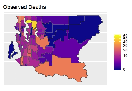
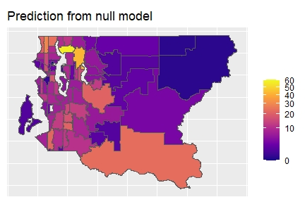
Figure 1: Left: observed COVID-19 deaths in King County, WA by ZIP code. Right: estimated COVID-19 deaths obtained by spatial smoothing, but with no covariates.

Data over a discrete spatial domain can be represented as observations $y_{i},i=1,\ldots,n$ on nodes of a graph $G_{n}=(V_{n},E_{n})$; here, the node set $V_{n}=\{1,\ldots,n\}$ corresponds to locations of observations and the edge set $E_{n}\subseteq V_{n}\times V_{n}$ contains undirected edges $(i,i^{\prime})$ among neighboring locations, $i\sim i^{\prime}$. The conditional autoregressive (CAR) model (Besag, 1974) and its intrinsic counterpart, the ICAR model (Besag and Kooperberg, 1995), provide an elegant framework for analyzing data over discrete spatial domains. In the simple case of Gaussian observations, the ICAR model assumes that the conditional mean of each $Y_{i}$ is the average of its neighbors in $G_{n}$. Formally, denoting by $n_{i}$ the number of neighbors of $i$,

$$Y_{i}\mid y_{i^{\prime}\neq i}\sim N\left(\sum_{i^{\prime}\sim i}\frac{y_{i^{\prime}}}{n_{i}},\,\frac{\tau^{2}}{n_{i}}\right),$$ (1)

where $\tau^{2}$ is the shared variance parameter. The correlations induced by ICAR model can be captured through a spatial random effect, leading to a linear mixed model that also includes fixed effect parameters corresponding to covariates of interest, as well as an additional noise term that captures the variation not explained by the spatial component. The model can also be extended to non-Gaussian observations through generalized linear mixed models (GLMMs). However, despite recent progress (e.g., Guan and Haran, 2018), handling non-Gaussian spatial observations using GLMMs remains challenging (Hughes, 2015).

Leveraging the conditional specification of probability distributions in CAR/ICAR, the BYM model of Besag et al. (1991) offers a flexible framework for spatial analysis using Bayesian hierarchical models, and is a popular choice for disease modeling. The prior specification of this model uses an ICAR component for spatial smoothing and an unstructured independent random effects component for location-specific noise. Various data distributions can be accommodated in this framework by considering a latent Gaussian process over the Markov random field specified by the graph $G_{n}$ (Rue and Held, 2005). The introduction of the integrated nested Laplace approximation (INLA; Rue et al., 2009) has further facilitated the use of this model and its extensions (Leroux et al., 2000; Dean et al., 2001). The BYM2 model proposed by Riebler et al. (2016) is a re-parameterization that improves interpretation of the model components, allowing for easier prior specification.

INLA offers considerable computational advantages, but the impact of its approximation on inference for fixed effect parameters is less clear. The recent implementation of the BYM2 model in stan (Morris et al., 2019) mitigates this issue at the cost of increased computational complexity. Practitioners are thus faced with a tradeoff between computation and validity and generality of inference. These challenges are compounded in the presence of high-dimensional covariates, which may occur when the relevant covariates cannot be scientifically determined; this is illustrated in Section 4.2, when we include a larger set of covariates when analyzing COVID-19 deaths in King County.

To overcome the above challenges, in this paper we develop a new doubly regularized generalized linear model (GLM) framework for analyzing spatial data on discrete domains with a large number of covariates. Our framework follows the same motivation as the CAR model (Besag, 1974), by encouraging similarity among outcomes in neighboring spatial regions in $G_{n}$. However, instead of introducing correlations among neighboring regions through spatial random effects, we use an over-parametrized spatial mean surface defined by region-specific intercepts, $\alpha_{i}$ for $i\in V_{n}$. More specifically, our first regularization encourages similarity among neighboring intercepts by using a network fusion penalty that encourages $\alpha_{i}\approx\alpha_{i^{\prime}}$ for neighboring nodes $i$ and $i^{\prime}$ in $G_{n}$ (Li et al., 2019). Our penalty corresponds to a discrete version of the Laplace-Beltrami operator (Wahba, 1981) on $G_{n}$. The Laplace-Beltrami operator defines thin-plate splines on manifolds (Duchamp and Stuetzle, 2003), which have a known connection to linear mixed models for Gaussian data (Ruppert et al., 2003), and are used as an alternative approach for analyzing spatial data (Cressie, 2015). Our approach is thus intimately related to commonly used approaches for analyzing spatial data; we further discuss the connection to mixed models in section C of the supplement. To facilitate inference for high-dimensional covariates ($p\gg n$), our approach also includes a second network regularization that encourages similarity among related covariates, as well as sparsity. Featuring a combination of $\ell_{1}$ and $\ell_{2}$ penalties, our doubly regularized GLM framework amounts to a convex optimization problem that can be solved efficiently for problems with large spatial domains (large $n$) and a large number of covariates (large $p$).

To infer the relevant covariates in a potentially high-dimensional model, we also develop an inference procedure for our doubly penalized generalized linear model. While our inference framework builds on recent developments in high-dimensional inference (van de Geer et al., 2014; Javanmard and Montanari, 2013), it is unique, as network penalty terms are generally not (semi)norms. This complicates the development of high-dimensional inference procedures. To overcome this challenge, we treat these non-norm penalty terms as part of the target loss function, which differs from the loss function minimized by the true population regression parameters. We control the distance between the target and true parameters, and then characterize the large sample behaviour of our proposed estimators. This approach allows us to incorporate partially uninformative or misspecified networks and still obtain valid inference for the association of features with the outcome. While penalized regression models have recently been developed for spatially correlated data (Cai et al. (2019); Chernozhukov et al. (2021)), our methods are the first, to our knowledge, to facilitate statistical inference for (non-Gaussian) generalized linear models.

We begin by describing our doubly-penalized regression methodology in Section 2, including algorithms for fitting the resulting models. We then give an overview of the theoretical details for our methods to obtain valid high-dimensional inference in Section 3. In Section 4, we analyze the King County COVID-19 death data. The results demonstrate that our method achieves good prediction, while identifying important covariates using the proposed inference procedure. Our simulation studies in Section 5 confirm that when the networks are informative, our method provides both improved prediction accuracy and inferential power. They also show that our method’s performances are robust to partially uninformative networks.

2 GLMs with Feature and Unit Network Kernels

Consider data consisting of $n$ observations $(y_{1},x_{1}),\dots,(y_{n},x_{p})$ where $y_{i}\in\mathbb{R}$ is the outcome and $x_{i}\in\mathbb{R}^{p}$ is the corresponding feature vector, centered and commonly scaled. We assume the conditional mean relationship between the outcomes and features is

$$\mathbb{E}[Y_{i}|X_{i}=x_{i}]=\mu(\alpha_{i}+x_{i}^{\prime}\beta),$$

where $\alpha_{i}\in\mathbb{R}$ are intercept terms for each unit $i$; $\beta\in\mathbb{R}^{p}$ is a vector of common regression coefficients; and $\mu$ denotes the inverse link function for the generalized linear model (GLM), which we will also refer to as the mean function. Examples of inverse canonical link functions used for generalized linear models include $\mu(x)=x$ for Gaussian models and $\mu(x)=\exp(x)(\exp(x)+1)^{-1}$ for binomial models.

We assume that observation units $i=1,\dots,n$ are connected on a known (weighted) graph $G_{n}=(V_{n},E_{n})$ where $V_{n}=\left\{1,\dots,n\right\}$ and $E_{n}\subset V_{n}\times V_{n}$ is a set of undirected edges $(i,i^{\prime})$ for $i\neq i^{\prime}$. A connection between two units $i$ and $i^{\prime}$ implies that they are likely to have similar outcomes $y_{i}$ and $y_{i^{\prime}}$. Let $w_{ii^{\prime}}\in\mathbb{R}^{+}$ denote the weight for each edge, which quantifies the strength of the similarity, and $A_{n}$ be the corresponding weighted adjacency matrix of $G_{n}$. Then, $L_{n}=D_{n}-A_{n}$ defines the graph Laplacian (Chung, 1997), where $D_{n}=\text{diag}(d_{1},\dots,d_{n})$ and $d_{i}=\sum_{i^{\prime}\in V_{n}}A_{ii^{\prime}}$. Our doubly penalized GLM framework encourages similarity among outcomes for neighboring nodes in $G_{n}$ by imposing a graph Laplacian penalty on the node-specific intercepts: $\alpha^{\prime}L_{n}\alpha=\sum_{i\sim i^{\prime}}w_{ii^{\prime}}\left(\alpha_{i}-\alpha_{i^{\prime}}\right)^{2}$. In order for the solution to be identifiable, we add an ordinary squared $\ell_{2}$ penalty on $\alpha$, i.e. penalizing $\|\alpha\|_{2}^{2}$. In application, these penalties are respectively similar to specifying an ICAR prior for spatial smoothing and independent random effects for non-spatial variance, as in the BYM model.

Our framework also features a second penalty, $P(G_{p},\beta)$, that incorporates known similarities among features $X_{j},j=1,\dots,p$, captured by graph $G_{p}=(V_{p},E_{p})$, when such information is available. We consider two possible choices of $P(G_{p},\beta)$: an $\ell_{2}$ penalty defined based on the graph Laplacian, and an $\ell_{1}$ penalty, as used in graph trend filtering (Wang et al., 2016). A connection between two features in $G_{p}$ implies that they have similar association with the outcome $y$. This type of smoothness has been previously leveraged by Li and Li (2008) and Zhao and Shojaie (2016). Defining $A_{p},D_{p},$ and $L_{p}$ analogously as above, the $\ell_{2}$ fusion penalty,

$$P(G_{p},\beta)=\frac{1}{2}\beta^{\prime}L_{p}\beta=\frac{1}{2}\sum_{j\sim j^{\prime}}w_{jj^{\prime}}(\beta_{j}-\beta_{j^{\prime}})^{2},$$

can be seen as a generalized ridge penalty that shrinks the weighted squared distance between connected features’ parameters towards zero. Similarly, the $\ell_{1}$ fusion penalty can also be seen as a generalized lasso penalty (Tibshirani et al., 2011). To this end, let $J_{p}$ be the incidence matrix of $G_{p}$, where each row of $J_{p}$ corresponds to an edge $(j,j^{\prime})$ in $G_{p}$, with element $j$ of the row having value $w_{jj^{\prime}}$ and element $j^{\prime}$ having value $-w_{jj^{\prime}}$ (in an unweighted graph, $J_{p}^{\prime}J_{p}=L_{p}$). Then, the $\ell_{1}$ fusion penalty can be written as

$$P(G_{p},\beta)=\|J_{p}\beta\|_{1}=\sum_{(i,j)\in E_{p}}w_{ij}|\beta_{i}-\beta_{j}|,$$

which encourages coefficients of graph-connected features to be exactly equal. Putting things together, the general form of our proposed estimator is given by

$$(\hat{\alpha},\hat{\beta})=\operatornamewithlimits{argmin}_{\alpha,\beta}\left\{\ell(y;\alpha+X\beta)+\frac{1}{2}\gamma_{n}\alpha^{\prime}(L_{n}+\delta I_{n})\alpha+\gamma_{p}P(G_{p},\beta)+\lambda\|\beta\|_{1}\right\},$$ (2)

where $\gamma_{n}$, $\gamma_{p}$, and $\lambda$ are positive tuning parameters; $\delta>0$ is a small fixed constant. Here, $X$ denotes the design matrix of observed features $x_{1},x_{2},\dots,x_{p}$.

The optimization problem (2) has four key components: (i) the loss function $\ell$ relates the outcome $y$ to the features $X$ while allowing for a unique intercept for each observation unit; (ii) the unit network smoothing penalty smooths $\hat{\alpha}$ over $G_{n}$; (iii) the feature network smoothing penalty smooths $\hat{\beta}$ over $G_{p}$; and (iv) the standard lasso penalty enforces sparsity on the features. The addition of the lasso penalty allows us to obtain sparse solutions in high dimensions, even when knowledge of similarity among features does not exist (i.e., $\gamma_{p}=0$). It also allows us to obtain asymptotic consistency for $\hat{\beta}$ at a rate that enables valid inference in high dimensions. We name this framework “generalized linear models with feature and unit network kernels”, or glm-funk, drawing from the nomenclature of kernels as similarity matrices (Randolph et al., 2018). Both of the glm-funk estimators described are computed by solving convex optimization problems, guaranteeing the existence of a global minimizer.

2.1 Optimization for $\ell_{2}$ feature network smoothing

To describe the algorithm for solving the glm-funk problem with $\ell_{2}$ feature network smoothing, we first rewrite the objective function in terms of $\theta:=(\alpha,\beta)^{\prime}$:

$$\hat{\theta}=\operatornamewithlimits{argmin}_{\theta\in\mathbb{R}^{n+p}}\left\{\ell\left(y;\tilde{X}\theta\right)+\frac{1}{2}\theta^{\prime}\tilde{L}\theta+\lambda\mathcal{R}(\theta)\right\},$$ (3)

where $\tilde{X}=[I_{n}\hskip 10.0ptX]$, $\mathcal{R}(\theta)=\|\beta\|_{1}$, and

$$\tilde{L}=\left[\begin{array}[]{cc}\gamma_{n}(L_{n}+\delta I_{n})&0\\ 0&\gamma_{p}L_{p}\end{array}\right].$$

Then, the optimization problem in (3) can be solved using a simple proximal gradient descent algorithm, given in Algorithm 1. In our simulations and data analysis, we use a fixed step-size of $\eta^{t}=0.001$, which provides reasonably fast convergence.

Define $\mathcal{L}(\theta):=\ell(y;\tilde{X}\theta)+\frac{1}{2}\theta^{\prime}\tilde{L}\theta$.;

Initialize $\theta^{0}$.;

for $t=0,1,\dots,$ until convergence of $\theta$ do

       Compute gradient, $\nabla\mathcal{L}(\theta^{t})=\tilde{X}^{\prime}\left(\mu(\tilde{X}\theta^{t})-y\right)+\tilde{L}\theta^{t}$.;

       Take a gradient step, $\tilde{\theta}=\theta^{t}-\eta^{t}\nabla\mathcal{L}(\theta^{t})$.;

       Take a proximal step,

$$\theta^{t+1}=\text{prox}(\tilde{\theta})=(\tilde{\theta}_{1},\dots,\tilde{\theta}_{n},S_{\lambda}(\tilde{\theta}_{n+1}),\dots,S_{\lambda}(\tilde{\theta}_{n+p}))^{\prime}$$

where $S_{\lambda}(x)=\text{sign}(x)\max(0,|x|-\lambda)$.;

      

end for

Result: $\hat{\theta}=\theta^{t+1}$

Algorithm 1 Proximal gradient descent for glm-funk with $\ell_{2}$ feature smoothing

2.2 Optimization for $\ell_{1}$ feature network smoothing

When using the generalized lasso penalty, the elements of $\beta$ are nonseparable in the penalty function. This leads to computational difficulties when using a non-identity GLM link function. To overcome this challenge, we solve an alternative problem, proposed by Chen et al. (2012), by replacing the generalized lasso penalty with a smooth $\ell_{\infty}$ approximation of the generalized lasso penalty:

$$f_{\tau}(\beta)=\max_{\|\nu\|_{\infty}<1}\left\{\nu^{\prime}J_{p}\beta-\tau\cfrac{1}{2}\|\nu\|_{2}^{2}\right\}.$$

Here, $\tau$ is a parameter that controls the approximation to the original $\ell_{1}$ problem; when $\tau=0$, $f_{\tau}(\beta)=\|J_{p}\beta\|_{1}$. Chen et al. (2012) prove that, for $\tau=\frac{\epsilon}{|E_{p}|}$, the absolute difference between optimal objective values of the original and approximate problems is upper bounded by $\epsilon$. The gradient of $f_{\tau}(\beta)$ is $J_{p}\nu^{*}$ where $\nu^{*}=S_{\infty}\left(\frac{\gamma_{p}J_{p}\beta}{\tau}\right)$, and $S_{\infty}$ is the element-wise projection operator onto the $\ell_{\infty}$ unit ball:

$$S_{\infty}(x)=\begin{cases}x,&\quad\text{for }-1\leq x\leq 1\\ 1,&\quad\text{for }x\geq 1\\ -1,&\quad\text{for }x\leq-1\end{cases}.$$

Replacing $\|J_{p}\beta\|_{1}$ with $f_{\alpha}(\beta)$, we can solve the approximate $\ell_{1}$ glm-funk problem using an accelerated proximal gradient descent algorithm (Beck and Teboulle, 2009). An adapted version of the algorithm presented in Chen et al. (2012) is given in Algorithm 2. In our simulations and data analysis, we set $\tau=0.001$, which provides sensible results, and a fast convergence rate.

Define $\mathcal{L}(\theta):=\ell(y;\tilde{X}\theta)+\frac{1}{2}\gamma_{n}\alpha^{\prime}(L_{n}+\delta I_{n})\alpha+\gamma_{p}f_{\tau}(\beta)$.;

Initialize $\theta^{0},w^{0}=\theta^{0},s^{0}=1$.;

for $t=0,1,\dots,$ until convergence of $\theta$ do

       Compute gradient,

$$\nabla\mathcal{L}(w^{t}):=\tilde{X}^{\prime}(\mu(\tilde{X}w^{t})-y)+[\gamma_{n}L_{n}w^{t}\hskip 10.0pt\gamma_{p}J_{p}^{\prime}\nu^{*}]^{\prime},$$

and the Lipschitz constant $C_{L}:=\|\nabla^{2}\mathcal{L}(w^{t})\|_{2}$.;

       Take a gradient step, $\tilde{\theta}=w^{t}-C_{L}^{-1}\nabla\mathcal{L}(\theta^{t})$.;

       Take a proximal step,

$$\theta^{t+1}=\text{prox}(\tilde{\theta})=\left(\tilde{\theta}_{1},\dots,\tilde{\theta}_{n},S_{\lambda/C_{L}}(\tilde{\theta}_{n+1}),\dots,S_{\lambda/C_{L}}(\tilde{\theta}_{n+p})\right)^{\prime},$$

where $S_{\lambda/C_{L}}(x)=\text{sign}(x)\max\left(0,|x|-\frac{\lambda}{C_{L}}\right)$.;

       Set $s^{t+1}=2/(t+3)$.;

       Set $w^{t+1}=\theta^{t+1}+\frac{1-s^{t}}{s^{t}}s^{t+1}(\theta^{t+1}-\theta^{t})$.;

      

end for

Result: $\hat{\theta}=\theta^{t+1}$

Algorithm 2 Accelerated proximal gradient descent for glm-funk with approximate $\ell_{1}$ feature smoothing

2.3 Prediction and tuning

Suppose we use $n_{\mathrm{trn}}$ observations for training the glm-funk model, and are interested in predicting outcomes for $n_{\mathrm{tst}}$ out-of-sample observations. In order to make predictions on out-of-sample data, we require an estimate of the unit-level intercepts $\alpha_{\mathrm{tst}}$. The test sample predictions are then given as $\mu(\hat{\alpha}_{\mathrm{tst}}+X\hat{\beta})$. Assuming we observe the entire network $G_{\mathrm{full}}$ connecting the $n_{\mathrm{trn}}+n_{\mathrm{tst}}$ units, we partition the Laplacian corresponding to $G_{\mathrm{full}}$ as:

$$L_{\mathrm{full}}=\left[\begin{array}[]{cc}L_{\mathrm{trn},\mathrm{trn}}&L_{\mathrm{trn},\mathrm{tst}}\\ L_{\mathrm{tst},\mathrm{trn}}&L_{\mathrm{tst},\mathrm{tst}}\end{array}\right]=\left[\begin{array}[]{cc}L_{11}&L_{12}\\ L_{21}&L_{22}\end{array}\right]$$

Then, we estimate $\alpha_{\mathrm{tst}}$ as in Li et al. (2019):

$$\hat{\alpha}_{\mathrm{tst}}=\operatornamewithlimits{argmin}_{\alpha_{\mathrm{tst}}}\left\{(\hat{\alpha}_{\mathrm{trn}},\alpha_{\mathrm{tst}})^{\prime}L_{\mathrm{full}}(\hat{\alpha}_{\mathrm{trn}},\alpha_{\mathrm{tst}})\right\}=-L_{22}^{-1}L_{21}\hat{\alpha}_{\mathrm{trn}}$$

Note that no network knowledge for the test observations (i.e. when the training and test units are disjoint on $G_{\mathrm{full}}$) corresponds to estimating $\hat{\alpha}_{\mathrm{tst}}=0$.

The glm-funk problems involve three tuning parameters $\gamma_{n}$, $\gamma_{p}$, and $\lambda$. We tune these jointly using $K$-fold cross-validation to minimize prediction error. Ideally, the $K$ folds would be determined using non-overlapping connected components of $G_{n}$, but this is not always possible for arbitrary networks. Due to the dependence among observation units over $G_{n}$, naïve cross-validation is not guaranteed to provide a good estimate of out-of-sample prediction error. However, as in Li et al. (2019), the procedure works relatively well in practice. While Rabinowicz and Rosset (2022) describe a method for cross-validation with correlated data, it requires the population covariance matrix, which we do not directly assume knowledge of. In order to efficiently determine the optimal tuning parameters, we use coordinate descent (Wright, 2015). Specifically, we optimize a single parameter (via $K$-fold cross-validation) while holding the others fixed, and cycle through all three parameters. In practice, this procedure usually converges in a very small number of coordinate descent iterations.

2.4 Related methods

As discussed in Section 1, spatial regression is commonly performed with Bayesian hierarchical models using priors to induce spatial smoothing. These models naturally require parametric assumptions, and can involve a trade-off between high computational complexity and validity of inference due to approximations used. In this section, we motivate our doubly regularized method by building on prior work in penalized regression over known network structures.

The recent proposal of Li et al. (2019) accounts for network structure among observation units by enforcing cohesion among the units. More specifically, it introduces the regression with network cohesion (RNC) model, which estimates unit-level intercepts subject to a cohesion penalty over $G_{n}$, by solving the optimization problem,

$$\min_{\alpha\in\mathbb{R}^{n},\beta\in\mathbb{R}^{p}}\left\{\ell(y;\alpha+X\beta)+\frac{1}{2}\gamma_{n}\alpha^{\prime}(L_{n}+\delta I_{n})\alpha\right\},$$

where $\ell$ is a loss function (usually the negative log-likelihood), and $\gamma_{n}>0$ tunes the strength of the penalty. The similarity between observations is captured through the $n$-dimensional intercept term $\alpha$. The addition of $\delta I_{n}$ for $\delta>0$ guarantees that a solution exists. The penalty term, which can be written as

$$\alpha^{\prime}(L_{n}+\delta I_{n})\alpha=\sum_{(i,i^{\prime})\in E_{n}}w_{ii^{\prime}}(\alpha_{i}-\alpha_{i^{\prime}})^{2}+\delta\sum_{i\in V_{n}}\alpha_{i}^{2},$$

implies that more strongly connected units are encouraged to have similar intercepts. This cohesion effect implies a similarity in outcomes independent of the features $X$; connected units may still differ in their values of $x_{i}^{\prime}\beta$. This is similar to incorporating variance components in a generalized linear mixed model, as further discussed in section C of the supplement. However, the RNC intercepts do not require distributional assumptions, and are specifically fit to optimize prediction power. Moreover, computation is much easier, as this problem is easily solved with standard convex optimization algorithms. Li et al. (2019) show that the RNC model improves prediction for network-linked observations compared to standard methods, while maintaining the interpretability of the fixed effects in standard generalized linear models. However, they do not discuss high-dimensional settings and statistical inference.

A similar choice for incorporating feature network structure is the Grace (graph-constrained estimation) penalty of Li and Li (2008), who proposed the estimator,

$$\hat{\beta}=\operatornamewithlimits{argmin}_{\beta\in\mathbb{R}^{p}}\left\{\ell(y;X\beta)+\frac{1}{2}\gamma_{p}\beta^{\prime}L_{p}\beta+\lambda\|\beta\|_{1}\right\},$$

where, as before, $\ell$ is a loss function, and $\gamma_{p},\lambda>0$ are penalty parameters. Unlike the RNC estimator, the Grace penalty is well-defined for high-dimensional settings, due to the regularization applied to the features. This penalized regression encourages cohesion among $\beta$ coefficients corresponding to connected features. The inclusion of an $\ell_{1}$ penalty also enforces sparsity in the solution $\hat{\beta}$. Zhao and Shojaie (2016) developed a significance test for Grace-penalized estimation, but their approach only applies to linear regression models. This similarly holds for the method of Chernozhukov et al. (2021), which extends LASSO-based inference to space-time correlated data.

Randolph et al. (2018) account for two-way structured data in a kernel-penalized linear regression model by solving

$$\hat{\beta}=\operatornamewithlimits{argmin}_{\beta}\left\{\|y-X\beta\|_{H}^{2}+\lambda\|\beta\|_{Q^{-1}}^{2}\right\},$$

where $H$ and $Q^{-1}$ are, respectively, $n\times n$ and $p\times p$ kernel matrices which summarize distances between the units and features. This can be thought of as fitting a generalized least squares (GLS) model subject to a generalized ridge penalty. Ignoring the $\ell_{1}$ penalty, we can consider the proposal of Li and Li (2008) to fall within this framework, using the graph Laplacian as a kernel. The RNC penalty of Li et al. (2019) is also similar to the first term in the kernel-penalized regression problem. Both methods penalize quantities that capture “left-over” variation from the features with respect to a unit distance matrix; in kernel-penalized regression, the distances between residuals $y-X\beta$ are penalized, while RNC penalizes the intercepts $\alpha$. However, GLS does not easily extend to non-Gaussian models. Therefore, in this paper, we apply the idea of kernel penalization to generalized linear models by unifying RNC and Grace-style penalties in high-dimensional settings. We also develop a statistical inference procedure that allows for valid hypothesis tests and confidence intervals for the regression coefficients, even when the networks are not fully informative.

3 Asymptotics and Inference

To assess the importance of covariates $X_{j},j=1,\dots,p$ for outcome $Y$ measured over a spatial domain, we are interested in obtaining valid inference for their corresponding regression coefficients $\beta$. Our estimator given in (2) is non-standard due to the use of the $n$-dimensional intercept term and penalty terms that are not semi-norms. In this section, we first investigate the large sample behaviour of $\hat{\beta}$ and $\hat{\alpha}$ estimated using the glm-funk estimator (2) with $\ell_{1}$ smoothing. We defer discussion of the estimator with $\ell_{2}$ smoothing (3) to the Supplementary Material. These results are then used to obtain a valid inference procedure for the true regression parameters.

3.1 Asymptotics

We begin by describing the assumptions required for our theoretical results to hold. First, we require that the outcomes $Y_{i}$ satisfy certain tail properties.

Assumption 1 (Tail behaviour).

One of the following holds:
(i) The centered observed outcomes $Y_{i}-\mathbb{E}[Y_{i}|X_{i}=x_{i}]=Y_{i}-\mu_{i}$ are uniformly sub-Gaussian, i.e.

$$\max_{i=1,\dots,n}K^{2}\mathbb{E}\left[\exp\left(\cfrac{(Y_{i}-\mu_{i})^{2}}{K^{2}}\right)-1\right]\leq\sigma^{2}_{0}.$$

for some constants $K,\sigma^{2}_{0}>0$.
(ii) The centered observed outcomes $Y_{i}-\mathbb{E}[Y_{i}|X_{i}=x_{i}]=Y_{i}-\mu_{i}$ are uniformly sub-exponential, satisfying

$$\max_{i=1,\dots,n}\|Y_{i}-\mu_{i}\|_{\psi_{1}}=K_{\psi_{1}}<\infty,$$

where

$$\|Y\|_{\psi_{1}}=\inf\left\{t>0:\mathbb{E}\exp(|Y|/t)\leq 2\right\}.$$

These tail conditions cover a large variety of common generalized linear models. Gaussian and binomial data satisfy the sub-Gaussian property, while Poisson and exponential outcomes have sub-exponential tails.

We further require some conditions on the loss function $\ell$ and the design matrix $X$.

Assumption 2 (Loss function properties).

The following hold:
(i) The loss function $\ell:\Theta\times\Omega\rightarrow\mathbb{R}$ is integrable over all $(X,y)\in\Omega$ for each $\theta\in\Theta$.
(ii) For almost all $(X,y)\in\Omega$, the derivative $\nabla_{\alpha}\ell$ exists for all $\alpha$.
(iii) There exists an integrable function $g:\Omega\rightarrow\mathbb{R}$ such that $|\ell(y;\tilde{X}\theta)|\leq g(X,y)$ for all $\theta\in\Theta$ and almost all $(X,y)\in\Omega$.
(iv) The conditional mean function $\mu$ and its derivative $\mu^{\prime}$ are Lipschitz continuous with constants $C_{\mu}<\infty$ and $C_{\mu^{\prime}}<\infty$.
(v) $\mu^{\prime}$ is uniformly bounded away from zero, that is, $|\mu^{\prime}(\cdot)|^{-1}\leq U^{\prime}<\infty$.

Assumption 3 (Design scaling).

The design matrix $X$ satisfies $|X_{ij}|\leq R<\infty$ for all $i,j$, and also scales as $\|X\|_{2}=o_{p}\left(\sqrt{\frac{n}{\log p}}\right)$.

The loss function assumptions are fairly mild, and common in the high-dimensional inference literature (van de Geer et al., 2014; Javanmard and Montanari, 2013; Bühlmann, 2013). The design scaling assumption is equivalent to assuming that the maximum eigenvalue of $X^{\prime}X$ grows at a rate slower than $n$, and can be shown to hold for various random designs (see Section 6.4 of Wainwright (2019)).

In order to state the remaining assumptions, we first define some quantities of interest. For a generic function $f$, let $\mathbb{P}f:=n^{-1}\sum_{i=1}^{n}\mathbb{E}[f(y_{i},x_{i})]$ and $\mathbb{P}_{n}f:=n^{-1}\sum_{i=1}^{n}f(y_{i},x_{i})$. Then, we rewrite our optimization problem as:

$$\hat{\theta}=\operatornamewithlimits{argmin}_{\theta}\left\{\mathbb{P}_{n}\mathcal{L}(\theta)+\lambda\mathcal{R}(\theta)\right\},$$

where $\mathcal{L}(\theta)=\ell(\alpha_{i}+x_{i}^{\prime}\beta)+\frac{1}{2}\gamma_{n}\alpha^{\prime}(L_{n}+\delta I_{n})\alpha$ and $\mathcal{R}(\theta)=\|\beta\|_{1}+\frac{\gamma_{p}}{\lambda}\|J_{p}\beta\|_{1}$. Our analysis involves two sets of parameters. The true parameter is defined as $\theta^{0}:=\operatornamewithlimits{argmin}_{\theta}\mathbb{P}\ell(\theta)$. We are interested in inference for the true parameter; however, theoretical results are difficult to directly obtain since the penalty involves terms which are not semi-norms. Therefore, we also work with the target parameter, which we define as $\theta^{*}:=\operatornamewithlimits{argmin}_{\theta}\mathbb{P}\mathcal{L}(\theta)$, where $\mathcal{L}$ includes the non-$\ell_{1}$ penalty terms.

It is important to note that our theoretical analysis is in a high-dimensional framework, where $n$ and $p(n)$ are both allowed to grow to infinity (and therefore, so are the dimensions of $\alpha$ and $\beta$). Hence, $\theta^{0}$ and $\theta^{*}$ are dependent on $n$ and $p$, and the following assumptions apply to a sequence of data-generating processes indexed by $(n,p)$. Our theoretical results then hold with high probability for large $(n,p)$. For ease of exposition, we do not include this dependence in our notations.

We make the following assumptions for estimation of the target and true regression parameters.

Assumption 4 (Compatibility condition).

Given a set $S\subset\left\{1,\dots,p\right\}$ with $|S|=s$, for all $c>0$ and for all $\theta=(\alpha,\beta)^{\prime}$ satisfying $\|\beta_{S^{c}}\|_{1}+c\|J_{p}\beta\|_{1}\leq\|\alpha\|_{1}+3\|\beta_{S}\|_{1}$, it holds that:

$$\cfrac{\|\alpha\|_{1}}{2}+\|\beta_{S}\|_{1}\leq\cfrac{\|\theta\|\sqrt{s}}{\phi(s)}$$

for some norm $\|\cdot\|$ and constant $\phi(s)>0$.

Assumption 5 (Restricted strong convexity).

For all $\theta=(\alpha,\beta)^{\prime}$ satisfying

$$\|\alpha-\alpha^{*}\|_{1}+\|\beta-\beta^{*}\|_{1}+\frac{\gamma_{p}}{\lambda}\left\|J_{p}\left(\beta-\beta^{*}\right)\right\|_{1}\leq M^{*},$$

with

$$M^{*}=\cfrac{16s\lambda^{2}}{\rho\phi^{2}(S)c}+\cfrac{2\gamma_{p}\|J_{p}\bar{\beta}\|_{1}}{\rho},$$

and $\lambda\geq 8\rho$, it holds that:

$$\mathbb{P}\left(\ell(\theta)-\ell(\theta^{*})\right)\geq\nabla\mathbb{P}\ell\left(\theta^{*}\right)^{\prime}\left(\theta-\theta^{*}\right)+G\left(\|\theta-\theta^{*}\|\right),$$

where $G(x)=cx^{2}$ for some constant $c>0$.

The compatibility and restricted strong convexity conditions are common in high-dimensional theory (Bühlmann and van de Geer, 2011). Intuitively, restricted strong convexity at the optimum $\theta^{*}$ means that the loss function is curved sharply around $\theta^{*}$. Hence, when $\mathbb{P}(\ell\left(\theta^{*}\right)-\ell(\theta))$ is small, so is $\|\theta^{*}-\theta\|$. Negahban et al. (2012) describe how this condition is needed for nonlinear models, and proved that it holds for various common loss functions in sparse high-dimensional regimes, including the logistic regression deviance.

Finally, we make assumptions on components of the true data-generating processes, and their relationship to the penalty parameters in the model.

Assumption 6 (Sparsity).

$\beta^{0}$ is $s$-sparse, that is, $\|\beta^{0}\|_{0}=s$ with $s=O_{p}\left(\sqrt{n}/\log p\right)$.

Assumption 7 (Penalty scaling).

The following hold:
(i) $\lambda=O_{p}\left(\sqrt{\frac{\log p}{n}}\right)$,
(ii) $\gamma_{p}\|J_{p}\beta^{0}\|_{1}=o_{p}(\lambda)$, and
(iii) $\gamma_{n}\|(L_{n}+\delta I)\alpha^{0}\|_{2}=O_{p}\left(n^{c}\right)$ where $c\in(0,\frac{1}{2})$.

The sparsity assumption and scaling condition of $\lambda$ are standard rates in the high-dimensional inference literature (van de Geer et al., 2014; Negahban et al., 2012).

Part (ii) of Assumption 7 allows us to not observe fully informative feature networks. It states that the quality of feature network smoothing is inversely proportional to the magnitude of its tuning parameter. That is, if the feature network is truly informative, we expect $\|J_{p}\beta\|_{1}\rightarrow 0$ (at a rate faster than $\lambda$), and $\gamma_{p}$ can be larger. In this scenario, the network structure impacts the $\beta$-penalization more than the lasso penalty. However, if the smoothing does not correspond to the true structure of $\beta$, then $\|J_{p}\beta^{0}\|_{1}$ will be far from zero, and $\gamma_{p}$ should tend to 0 at a rate faster than $\|J_{p}\beta^{0}\|_{1}^{-1}$. In addition, if the feature network is uninformative, then $\gamma_{p}$ also needs to go to 0 faster than $\lambda$. In this case, most of the penalization is driven by the lasso penalty, rather than the network structure encoded by $J_{p}$. The empirical results in Section 5 suggest that our cross-validation approach achieves these properties data-adaptively.

Part (iii) of Assumption 7 similarly allows for some degree of non-informativeness in the unit network, and is also necessary to establish control of $\|\alpha^{*}-\alpha^{0}\|$. It establishes the trade-off needed between the unit network parameter $\gamma_{n}$ and the ridge penalty parameter $\delta$; if the unit network is informative and $\gamma_{n}$ is large, then $\delta$ should shrink to 0.

Under these assumptions, we can prove that $\hat{\beta}$ and $\hat{\alpha}$ tend to the target parameters $\beta^{*}$ and $\alpha^{*}$ in $\ell_{1}$ norm.

Theorem 1 (Consistency).

Under Assumptions 1-7, we have that

$$\|\hat{\alpha}-\alpha^{*}\|_{1}+\|\hat{\beta}-\beta^{*}\|_{1}=O_{p}\left(\lambda+\cfrac{\gamma_{p}}{\lambda}\|J_{p}\beta^{*}\|_{1}\right).$$

The proof, given in the Supplementary Material, follows a similar argument as the proof for generalized sparse additive models in Haris et al. (2019). A key difference in our theory is handling the $n$-dimensional intercept term $\alpha$, and its corresponding $\ell_{2}$ penalty. We also prove the result for outcome distributions which are not sub-Gaussian, such as Poisson and exponential data.

This result allows for consistent estimation of the target parameters $\beta^{*}$ and $\alpha^{*}$. In the Supplementary Material, we show that $\beta^{*}$ is the same as $\beta^{0}$, and the bias of $\alpha^{*}$ relative to $\alpha^{0}$ is controlled. This allows for us to obtain valid inference for the true $\beta^{0}$, under our procedure which we describe in the next section.

3.2 Inference

We now describe a statistical inference procedure for the $\beta$ parameters in the glm-funk model. We are specifically interested in testing the individual association between outcome $y$ and feature $X_{j}$ conditional on the other features $X_{-j}$. This corresponds to the null hypotheses $H_{0,j}:\beta_{j}=0$ for $j=1,\dots,p$. Classical inference theory does not directly apply in the high-dimensional setting. Instead, high-dimensional inference approaches generally either involve post-selection procedures, potentially via sample splitting (Wasserman and Roeder, 2009; Lee et al., 2016), or constructing an asymptotically unbiased estimator from the optimal solution $\hat{\beta}$ (Dezeure et al., 2015). We focus on the latter approach, known as de-biasing.

Several de-biasing procedures have been developed, including the low-dimensional projection estimator by Zhang and Zhang (2014), the ridge projection estimator by Bühlmann (2013), and the desparsified lasso estimator by van de Geer et al. (2014). These methods generally consider regression models with an ordinary ridge or lasso penalty only. The Grace test by Zhao and Shojaie (2016) specifically provides inference for linear regression with the $\ell_{2}$ Laplacian penalty. However, this method does not account for unit-level networks, and does not extend to the case of generalized linear models.

We consider the de-biased estimator of Javanmard and Montanari (2013), which easily extends to generalized linear models. Our de-biased estimator is defined as:

$$\hat{b} =\hat{\beta}-n^{-1}MX^{\prime}(\mu(\hat{\alpha}+X\hat{\beta})-y),$$

where $M$ is an estimate of the inverse of $\hat{\Sigma}:=\frac{1}{n}\nabla^{2}\ell(\hat{\alpha}+X\hat{\beta})$. The sandwich estimator of the variance-covariance matrix may also be used here. Note that in the case of Gaussian linear models, $\hat{\Sigma}$ requires a consistent estimator of $\sigma$, the noise standard deviation; the scaled lasso estimator of Sun and Zhang (2012) can be used for this. $M$ is computed by solving an optimization problem where $\|\hat{\Sigma}M-I_{p}\|_{\infty}$ is minimized. Specifically, for each $j=1,\dots,p$, the $j$-th column of $M$, $m_{j}$, is defined as the solution to

$$\min_{m\in\mathbb{R}^{p}}m^{\prime}\hat{\Sigma}m\hskip 10.0pt\text{subject to}\hskip 10.0pt\|\hat{\Sigma}m-e_{j}\|_{\infty}\leq q,$$

where $e_{j}\in\mathbb{R}^{p}$ is the $j$-th basis vector. The next result shows that under the assumptions described previously, we obtain an asymptotic distribution suitable for inference.

Theorem 2 (Asymptotic Normality).

Under the conditions of Theorem 1, as $n\longrightarrow\infty$,

$$\sqrt{n}\left(\hat{b}-\beta^{0}\right)\longrightarrow_{d}N\bigg{(}0,n^{-1}M\mathbb{E}\left[\nabla\ell(\alpha^{0}+X\beta^{0})\nabla\ell(\alpha^{0}+X\beta^{0})^{\prime}\right]M\bigg{)}.$$

In the proof, given in the Supplementary Material, we establish that the target $\beta^{*}$ is the same as the true $\beta^{0}$, and derive an asymptotic rate for $\|\alpha^{*}-\alpha^{0}\|_{1}$. We then apply Theorem 1 to show the result. As a result, even though our target parameter $\theta^{*}$ is different from $\theta^{0}$, Theorem 2 facilitates valid inference for the true regression parameters $\beta^{0}_{j}$. Specifically, we use the corresponding test statistic:

$$T_{j}=\cfrac{\sqrt{n}\hat{b}_{j}}{[M\hat{\Sigma}M]_{jj}^{1/2}},$$

and 100(1 - $\alpha$)$\%$ confidence interval:

$$\hat{b}_{j}\pm q_{(1-\frac{\alpha}{2})}n^{-1/2}[M\hat{\Sigma}M]_{jj}^{1/2}.$$

4 Analysis of King County COVID-19 Data

In this section, we analyze novel coronavirus (COVID-19) death counts in King County, WA, obtained September 14, 2020. We incorporate geographical, demographic and socioeconomic information from King County GIS Open Data along with the list of long-term care facilities being monitored for COVID-19. We model the spatial domain as an unweighted graph whose nodes are the ZIP codes (83 total for which COVID-19 data is available) in King County; two nodes are connected if they have overlapping borders. The outcome of interest is the total number of residents at each ZIP code who have died due to COVID-19.

We conduct two analyses both using a Poisson generalized linear model with ZIP code population as an offset, and compare results from our models with those from the state-of-the-art BYM2 model (Riebler et al., 2016), implemented with integrated nested Laplace approximation (INLA) (Rue et al., 2009; Lindgren and Rue, 2015). In our first analysis (Section 4.1), we consider a small number of covariates without including the feature kernel penalty $P(G_{p},\beta)$, i.e., we set $\gamma_{p}=0$. In our second analysis (Section 4.2), we include a larger number of covariates and demonstrate the utility of the feature kernel penalty, $P(G_{p},\beta)$ in fusing the parameters for related covariates.

4.1 COVID-19 model without feature network penalty

Covariates included in this analysis are race distribution (proportions of Black, White and Asian populations), median household income, education status (proportion of residents with college degree or above), age distribution (proportions of residents in four age groups: 18-29, 30-44, 45-59 and over 60), proportion of residents with medical insurance, number of hospitals, population density, number of King County Metro transit stops (as proxy for residential vs commercial neighborhood), and the number of nursing homes being monitored, each summarized on the ZIP code level.

Covariates represented by proportions of different categories, such as race and age, are relative abundances. To mitigate the effect of spurious correlations in these compositional data, we use the additive log-ratio transformation (Aitchison, 1982), omitting one category (e.g. age group below 18 and races other than Black, White or Asian). Figure 2 presents the distribution of race (untransformed), income, nursing homes and the number of deaths. The plots highlight correlations between race and income, and between the number of nursing homes and deaths.

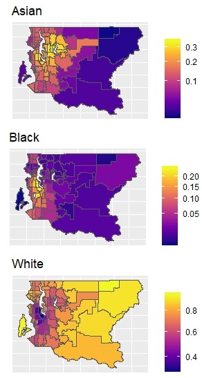
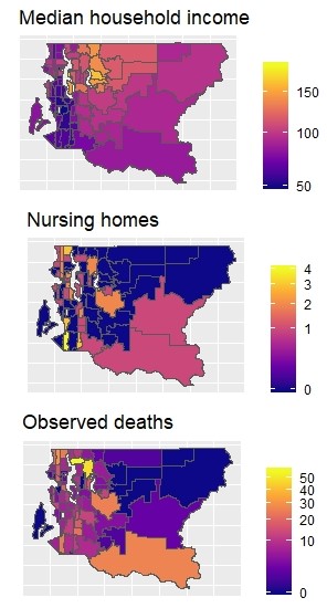
Figure 2: Distribution of race (proportions), income (median), nursing homes (count) and COVID-19 deaths by ZIP code.

In addition to the ‘full’ glm-funk model, which utilizes the spatial graph structure and the above covariates, and the ‘null’ spatial smoothing model with no covariates visualized in Section 1, we consider two benchmark models that ignore the spatial graph structure and treat all ZIP codes as independent. One removes the graphical fusion term and assigns a common intercept to all regions, similar to a traditional Poisson GLM. The other fits individual intercepts penalized towards zero, i.e. where $L_{n}=0$. The tuning parameters $\gamma_{n}$ and $\lambda$ are selected via 10-fold cross-validation. We randomly assign the cross-validation folds under the constraint that no adjacent regions can be assigned to the same test set. This is due to the relatively small sample size and the variability in the observations, especially for regions that are far apart. We use the estimates from the independent model with a common intercept as initial values for optimization when fitting the other two models, to obtain more stable solutions from the optimization with limited sample size.

We also compare the proposed model with the BYM2 model (Riebler et al., 2016), which is a modified version of the Besag-York-Mollié (BYM) model (Besag et al., 1991). The BYM2 model specifies the linear predictor as $\log\mathbb{E}[Y_{i}]=\log P_{i}+\alpha+X_{i}\beta+\left[\sqrt{\rho/s}\cdot\phi_{i}+\sqrt{1-\rho}\cdot\theta_{i}\right]\sigma$, where $P_{i}$ is the offset, $\phi_{i}$ corresponds to the spatially correlated errors, and $\theta$ reflects non-spatial heterogeneity. For the error term, $\sigma$ is the overall standard deviation, $\rho\in[0,1]$ controls the proportion of spatial and non-spatial errors, and the scaling factor $s$ is directly determined by the graph Laplacian such that $\text{Var}(\phi_{i}/\sqrt{s})\approx 1$ for each $i$. We conduct Bayesian inference for this model with the R-INLA package (Lindgren and Rue, 2015). The performance of all models is assessed by the negative log-likelihood with 10-fold cross-validation.

Figure 3 visualizes the residuals from each model, and reports their negative log-likelihood evaluated on the validation sets. Roughly, the former reflects the bias of each model, while the latter shows the overall accuracy. The full glm-funk model achieves better model fit than other models, and BYM2 has a relatively high loss (negative log-likelihood) due to the large variability in its predictions (ranging from 14.3 to beyond 1000 across 10 CV folds). The residual plots show that the full glm-funk model and the independence model with individual intercepts achieve lower biases in their predictions by allowing each region to have an individual baseline risk. The former achieves lower negative log-likelihood by accounting for the similarity between adjacent regions based on the spatial graph structure, trading off some region-specific bias.

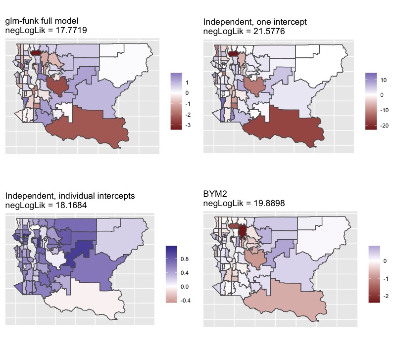
Figure 3: Residuals from each model, with cross-validated negative log-likelihood reported in the titles.

In addition to cross-validated negative log-likelihood, we also compare the models in terms of estimated effect sizes (rate ratios). Table 1 shows the effect sizes (posterior mean is used for the BYM2 model) along with 95$\%$ confidence intervals (for non-Bayesian models) or credible intervals (for BYM2) of the covariates in each model. The effect sizes are reported on the scale of standardized and transformed covariates. The full glm-funk model results highlight the proportion of senior population and the number of nursing homes as being significant covariates. The independent model with one intercept identifies the majority of covariates to be statistically significant, except for the proportion of White population and the number of transit stops. The independent model with region-specific intercepts, in contrast, does not find any covariate effect to be significant. Such observation aligns with our intuition that the one-intercept independence model attributes more heterogeneity in the outcome to the covariates, while the individual-intercept model captures more variability through the spatially-varying intercepts. glm-funk achieves a balance between them by specifying region-specific, but spatially-fused intercepts. The significance of senior population and the number of nursing homes identified by glm-funk matches our expectation and knowledge for COVID-19, and the correlation between the number of deaths and the number of nursing homes shown in Figure 2. The BYM2 model does not identify any significant covariates, and tends to provide wider credible intervals compared to the frequentist methods; this reflects greater uncertainty in the estimates made by the BYM2 model, especially with small to moderate sample sizes as in our example. As we will demonstrate in Section 5, the BYM2 model could be more conservative when the signal-to-noise ratio is low.

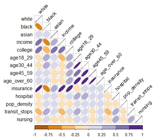
Figure 4: Correlation between transformed covariates. Purple and orange color correspond to positive and negative correlation, respectively. The shade and shape reflect the magnitude of correlation.

Table 1: Rate ratios and 95$\%$ confidence/credible intervals (CI/CrI) for each model. Rate ratios correspond to standardized and transformed covariates.

	Full	Independent, one intercept	Independent, individual intercepts	BYM2
	RR (95% CI)	RR (95% CI)	RR (95% CI)	RR (95% CrI)
Race
White	0.99 (0.95, 1.04)	1.00 (0.96, 1.05)	1.00 (0.96, 1.04)	0.73 (0.24, 2.23)
Black	1.00 (0.94, 1.06)	0.67 (0.63, 0.72)	1.00 (0.94, 1.06)	0.62 (0.27, 1.38)
Asian	1.00 (0.94, 1.06)	1.42 (1.33, 1.52)	1.00 (0.94, 1.06)	1.71 (0.72, 4.13)
Income	0.99 (0.95, 1.04)	0.90 (0.86, 0.94)	1.00 (0.95, 1.04)	0.46 (0.10, 2.14)
College education	1.00 (0.96, 1.04)	0.63 (0.60, 0.65)	1.00 (0.96, 1.04)	0.85 (0.18, 4.00)
Age
18-29	1.01 (0.96, 1.05)	0.27 (0.26, 0.28)	1.00 (0.96, 1.05)	0.56 (0.11, 2.90)
30-44	1.01 (0.97, 1.06)	4.03 (3.85, 4.21)	1.00 (0.96, 1.05)	0.74 (0.10, 5.64)
45-59	1.01 (0.96, 1.05)	0.53 (0.51, 0.56)	1.00 (0.96, 1.05)	0.95 (0.10, 7.92)
>60	1.13 (1.08, 1.19)	2.18 (2.08, 2.28)	1.01 (0.97, 1.06)	3.14 (0.58, 17.73)
Medical insurance	1.00 (0.95, 1.04)	0.83 (0.80, 0.87)	1.00 (0.96, 1.04)	1.40 (0.34, 5.69)
Hospitals	1.01 (0.94, 1.08)	1.12 (1.05, 1.19)	1.00 (0.93, 1.07)	1.00 (0.63, 1.60)
Population density	0.92 (0.76, 1.10)	0.59 (0.41, 0.86)	0.95 (0.78, 1.15)	0.76 (0.42, 1.21)
Transit stops	1.02 (0.96, 1.09)	0.98 (0.92, 1.04)	1.00 (0.94, 1.06)	0.91 (0.49, 1.71)
Nursing homes	1.28 (1.22, 1.36)	1.28 (1.20, 1.36)	1.04 (0.97, 1.10)	1.37 (0.88, 2.13)

4.2 COVID-19 model with feature network penalty

In our first analysis in Section 4.1, we identified a subset of covariates to include in the model based on the current knowledge of COVID-19 pandemic. This is clearly the right approach if such knowledge exists. However, even in well-studied cases, such as COVID-19, we may not be able to fully identify the relevant covariates that need to be included in the analysis.

To illustrate the full capabilities of our doubly-regularized approach, in this section we take such an approach and include additional features in the model. More specifically, in addition to the covariates considered in Section 4.1, our expanded analysis includes three types of additional features, namely, environmental variables (proportion of medium and high basins, erosion hazard and landslide hazard), public facilities (number of schools, solid waste facilities and veterans, seniors and human services levy) and public safety facilities (number of fire stations and police stations). These covariates are less related to COVID-19 deaths based on our current knowledge, and so we investigate whether our model estimates are robust against the inclusion of potentially weak predictors.

The proposed glm-funk framework with both unit and feature network penalties allows us to encourage similarity among coefficients associated with covariates in each of the three new groups of features (environmental, public facility and public safety) through a feature network $G_{p}$ in which features in the same category are connected. We report results for both the $\ell_{1}$ and the $\ell_{2}$ fusion penalty. Table 2 summarizes the estimates, confidence intervals and p-values for these models. Estimates and credible intervals from the BYM2 model are presented as a comparison. Figure 5 visualizes the residuals from each model, and reports the corresponding negative log-likelihood on validation sets from 10-fold CV. Since predictions from the BYM2 model have large variability across the 10 CV folds as in Section 4.1, we report its median negative log-likelihood instead.

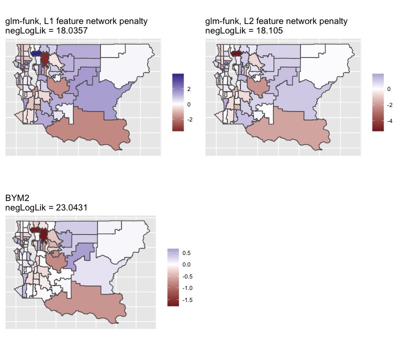
Figure 5: Residuals from each model with added covariates, with cross-validated negative log-likelihood reported in the titles.

Table 2: Debiased estimates and 95% confidence/credible intervals
from the proposed model with feature network penalty and from the BYM2 model

	glm-funk, $\ell_{1}$		glm-funk, $\ell_{2}$		BYM2
	RR (95% CI)	p-value	RR (95% CI)	p-value	RR (95% CrI)
Race
White	0.91 (0.87, 0.95)	<0.001	0.90 (0.86, 0.94)	<0.001	0.74 (0.18, 3.00)
Black	1.09 (1.01, 1.17)	0.019	1.07 (0.99, 1.15)	0.076	0.63 (0.25, 1.55)
Asian	1.00 (0.94, 1.06)	0.950	1.00 (0.94, 1.06)	0.963	1.61 (0.55, 4.82)
Income	0.96 (0.92, 1.01)	0.090	0.97 (0.92, 1.01)	0.129	0.42 (0.07, 2.71)
College education	1.00 (0.95, 1.05)	0.972	0.99 (0.94, 1.04)	0.609	1.00 (0.09, 10.52)
Age
18-29	1.02 (0.97, 1.06)	0.485	1.01 (0.97, 1.06)	0.553	0.59 (0.09, 3.89)
30-44	1.01 (0.97, 1.06)	0.524	1.03 (0.99, 1.08)	0.173	0.63 (0.06, 6.36)
45-59	1.01 (0.96, 1.05)	0.803	1.01 (0.96, 1.05)	0.815	1.17 (0.07, 18.03)
>60	1.01 (0.97, 1.06)	0.596	1.02 (0.98, 1.07)	0.374	2.81 (0.32, 25.33)
Medical insurance	0.92 (0.88, 0.96)	<0.001	0.91 (0.87, 0.95)	<0.001	1.43 (0.25, 8.00)
Hospitals	0.99 (0.93, 1.07)	0.873	1.01 (0.94, 1.09)	0.782	0.98 (0.56, 1.74)
Population density	0.92 (0.78, 1.09)	0.352	0.88 (0.71, 1.09)	0.242	0.75 (0.38, 1.31)
Transit stops	1.04 (0.96, 1.13)	0.341	1.05 (0.96, 1.14)	0.275	0.91 (0.34, 2.40)
Nursing homes	1.37 (1.28, 1.48)	<0.001	1.37 (1.27, 1.47)	<0.001	1.41 (0.80, 2.50)
Environmental
Basin medium	0.98 (0.88, 1.08)	0.625	0.99 (0.90, 1.10)	0.881	1.13 (0.38, 3.36)
Basin high	0.97 (0.86, 1.09)	0.564	0.94 (0.83, 1.05)	0.267	0.69 (0.19, 2.42)
Erosion hazard	0.99 (0.94, 1.04)	0.800	1.01 (0.95, 1.07)	0.864	1.06 (0.46, 2.46)
Landslide hazard	1.01 (0.93, 1.11)	0.764	0.99 (0.90, 1.08)	0.809	1.18 (0.54, 2.58)
Public facility
School	1.00 (0.92, 1.09)	0.993	1.00 (0.92, 1.09)	0.962	1.00 (0.50, 2.04)
Solid waste	0.99 (0.91, 1.08)	0.872	0.99 (0.91, 1.08)	0.878	1.02 (0.60, 1.75)
Veteran	0.98 (0.88, 1.08)	0.640	0.98 (0.89, 1.09)	0.750	0.93 (0.47, 1.83)
Public safety
Fire	1.00 (0.92, 1.08)	0.949	1.02 (0.94, 1.10)	0.647	1.08 (0.56, 2.12)
Police	1.01 (0.92, 1.11)	0.803	1.01 (0.93, 1.09)	0.877	1.07 (0.56, 2.05)

As we may expect, the added environmental, public facility and public safety variables are not identified as important predictors of COVID-19 death rates. The proposed glm-funk model with both $\ell_{1}$ and $\ell_{2}$ feature network penalty outperformed BYM2 model in terms of cross-validated negative log-likelihood. With the inclusion of additional features, the BYM2 model still identifies no important predictor for COVID-19 deaths. For the glm-funk models, the statistical significance for the majority of predictors remains unchanged, while the proportion of senior population is no longer a significant covariate for the glm-funk models, and medical insurance coverage and race distribution are identified as significant instead.

Such observation indicates that glm-funk is slightly sensitive to the inclusion of spatially structured (and likely less relevant) variables; we discuss this further in Section 6. The importance of race matches our knowledge of COVID-19 burden (Price-Haywood et al., 2020), and the insignificance of age (for the $>60$ age group) may be due to the presence of nursing homes as a significant variable in the model. Figure 4 shows that medical insurance is correlated with multiple socio-demographic variables. On the one hand, this high correlation explains the importance of medical insurance as a predictor in the glm-funk model, potentially as a surrogate for other important variables, and, on the other, serves as a reminder for not over interpreting the results.

5 Simulation Studies

5.1 Simulation settings

In this section, we evaluate the performance of the proposed glm-funk models using simulated spatial data. We generated count responses from the model

$$Y\sim\text{Poisson}(\exp(\alpha+X\beta)),$$

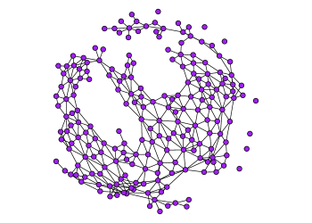
Figure 8: Spatial lattice corresponding to $204$ King County and surrounding area ZIP codes.

where $\alpha$ denotes a region-specific random intercept, over a discrete spatial lattice based off the geography of King County and surrounding areas. The spatial lattice graph of these 204 regions (including ZIP codes where COVID-19 data was unavailable for our data analysis in Section 4) is shown in Figure 8 in the Supplementary Material.

Using the method of Rue and Held (2005), we generated the spatial random effects $\alpha_{i}$ according to an ICAR model as in Equation (1) for $i=1,\dots,n$, with $\tau=1$. For the fixed effects, we set $\beta_{1}=\cdots=\beta_{\frac{s}{2}}=\rho$, $\beta_{\frac{s}{2}+1}=\cdots=\beta_{s}=-\rho$, and the remaining coefficients to 0; we vary the absolute effect size $\rho$ across simulations. The feature graph $G_{p}$ is set to have $2p/s$ disconnected components of size $s/2$ each. Each component has a single hub node which is connected to the remaining non-hub nodes that do not have any other connections. In generating the features $X$, each hub node feature is generated as $x_{h}\sim N(0,1)$, with connected non-hub features generated as $x_{nh}\sim N(0.35x_{h},1)$. This setup is similar to that of the simulations in Li and Li (2008).

We consider high-dimensional covariate spaces under the data-generating process specified above. We also consider the setting where the networks $G_{n}$ and $G_{p}$ are not fully informative, to assess the robustness of our method.

5.2 Simulation results

For this simulation study, we set $p=300$ and $s=20$. For $G_{n}$, we use the King County spatial lattice directly, resulting in $n=204$ regions. We replace the Bayesian BYM2 model with Li et al. (2019)’s RNC model with a lasso penalty (i.e. glm-funk with $\gamma_{p}=0$) in order to demonstrate the performance of a model that only accounts for structure among $G_{n}$. Note that while Li et al. (2019) do not include inference for high-dimensional $\beta$ parameters, this can be obtained as a special case of our method. Similarly, we consider a lasso-penalized Poisson regression as a model that does not account for network structure in either the regions or features.

Results for this simulation setting are shown in Figure 6. We observe that the glm-funk models outperform the models which do not incorporate the feature network information in terms of power. Comparing glm-funk with $\ell_{1}$ and $\ell_{2}$ smoothing, we see that the $\ell_{1}$ model achieves the highest power, which makes sense since the connected $\beta$ coefficients are exactly equal to each other. For out-of-sample predictive performance, these models perform the best when the signal strength of the features is high. The $\ell_{1}$ model in particular shows meaningfully better predictions, and also better coverage probability.

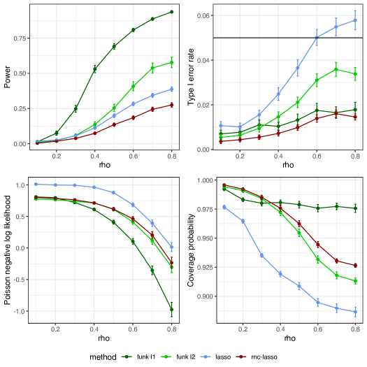
Figure 6: High-dimensional simulation results for fully informative networks. Means over 100 replicates are displayed with standard error bars. Left: power, middle: Type I error rate, right: test set root mean squared error.

5.3 Partially uninformative networks

We now examine the effect of modeling with partially uninformative networks in the high-dimensional setting. For $G_{p}$, we randomly add intra-component edges to the original network with constant probability 0.002 among all possible edge pairs. In our simulations, this corresponds to 87 additional edges in $G_{p}$ (32% of edges uninformative) on average. These uninformative edges encourage intercepts from different blocks or $\beta$ coefficients from different components to be close to each other. For $G_{n}$, we generate the region-specific intercepts independently from a $N(0,0.24)$ distribution, matching the mean and standard deviation of $\alpha$ in the previous simulation study. Here, the ICAR model does not apply, and spatial smoothing should not be helpful.

Results for this setting are shown in Figure 7. Given partial noise in the network adjustments, the proposed methods show robust results. Here, the glm-funk models still have the highest power, though attenuated relative to the fully informative setting. Their predictive accuracy and coverage probabilities are also reduced, though the $\ell_{1}$ model still shows an advantage to others.

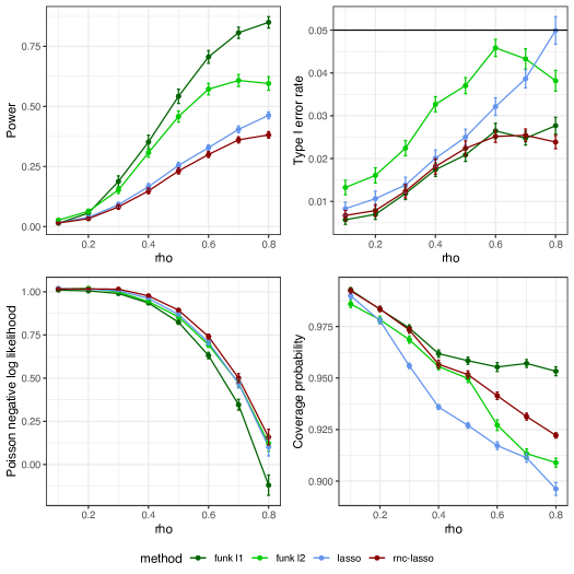
Figure 7: High-dimensional simulation results for partially uninformative networks. Means over 100 replicates are displayed with standard error bars. Left: power, middle: Type I error rate, right: test set root mean squared error.

6 Discussion

Motivated by applications in spatial disease modeling, we have developed a new framework for analyzing data with network structure among both observations and features. Using doubly regularized generalized linear models, we also obtained valid high-dimensional inference for our model parameters, under potentially informative network structure. The proposed methodology—which is implemented in the R package glmfunk, available on GitHub—can also be used in other applications involving doubly-structured data. Examples include analysis of microbiome data (Randolph et al., 2018) and multi-view omics data integration (Li et al., 2018).

Similar to approaches based on spatial random effects, our approach is not immune to the challenges of inference for fixed effect parameters due to spatial confounding (Reich et al., 2006). However, our empirical results suggest that our data-adaptive regularization and the additional ridge penalty discussed in Section 2 lessens the confounding effect. The results from analyzing the well-studied Slovenian cancer data set are case in point: Using a nonspatial GLM with Poisson link, the estimate of the effects of socioeconomic score is $\hat{\beta}=-0.14$ with 95% CI: ($-0.18$, $-0.10$). This is very similar to the results reported in Hodges and Reich (2010) who report the posterior mean and 95% credible intervals $-0.14$ and ($-0.17,-0.10$). Hodges and Reich (2010) report attenuated fixed effect estimate when adding the spatial random effects using the BYM model—posterior mean -$0.02$ and 95% credible interval ($-0.10,0.06$). Thus, in this case, the addition of spatial random effect amounts to a qualitative change in the importance of the socioeconomic score. In contrast, while the fixed effect parameter is also attenuated in the spatial version of our Poisson GLM—$\hat{\beta}=-0.09$ and 95% CI ($-0.15,-0.04$)—the spatial confounding seems to be less severe. As a result, the two models offer qualitatively similar conclusions.

When the networks are informative for the true data-generating process, we expect our method to show improved prediction and inference compared to standard high-dimensional methods. When the networks are misspecified or uninformative, our theoretical analysis suggests that the method should still achieve consistent estimation and valid inference for the true regression parameters, if appropriate penalty parameter scaling is used. However, tuning the network penalty parameters to achieve this in practice may be difficult, as naïve cross-validation is not guaranteed to be successful, given the dependencies among the observation units. An area for future research would be to incorporate cross-validation for correlated data (similar to e.g. Rabinowicz and Rosset (2022)) that is compatible with our method. Although we only considered Laplacian and graph incidence matrices in this paper, other kernels can easily be used within the glm-funk model. Another possibility would be to avoid adding unit-level intercepts, and instead penalizing the fitted values $X\beta$ directly; that is, using the penalty $\gamma_{n}\beta^{\prime}X^{\prime}L_{n}X\beta$.

SUPPLEMENTARY MATERIAL

Appendix A Technical proofs

Here, we prove the results in Section 3. We begin by comparing the target parameters $\theta^{*}$ to the true parameters $\theta^{0}$, showing that $\beta^{*}=\beta^{0}$ and establishing a bound on $\|\alpha^{*}-\alpha^{0}\|_{2}$. We then focus on estimation of the target $\theta^{*}$ using the $\ell_{1}$-regularized $\hat{\theta}$. We derive tail bounds on the empirical process term under both sub-Gaussian and sub-exponential outcomes, which are then used to show $\hat{\theta}\rightarrow\theta^{*}$ in $\ell_{1}$ norm. Our proof of Theorem 1 is similar to that of Theorem 3 in Haris et al. [2019], which provides fast rates of convergence for generalized sparse additive models. A key step in the proof by Haris et al. [2019], which differentiates it from a similar one in Bühlmann and van de Geer [2011], is handling an intercept term which is not penalized. We extend this to our setting, with an $n$-dimensional intercept term that is $\ell_{2}$ penalized. We then prove Theorem 2, which shows the validity of our de-biased estimator $\hat{b}$ for inference on the true $\beta^{0}$.

Target vs. true parameters

We first compare the target parameters $\theta^{*}$ to the true parameters of interest $\theta^{0}$. We start by noting that the target $\beta^{*}$ is the same as the true $\beta^{0}$. Using this fact, we characterize the difference in the target and true intercepts; that is, $\|\alpha^{*}-\alpha^{0}\|$.

Lemma 1.

The target parameter $\beta^{*}$ is equal to the true parameter $\beta^{0}$.

Proof.

This follows immediately by examining the $\beta$-optimality conditions for both objective functions,

$$0 =\nabla_{\beta}\mathbb{E}[\ell(\alpha^{*}+X\beta^{*})]$$

$$0 =\nabla_{\beta}\mathbb{E}[\ell(\alpha^{0}+X\beta^{0})],$$

and by convexity of the loss function. ∎

Lemma 2.

Under Assumptions 2 and 7, $\|\alpha^{*}-\alpha^{0}\|_{2}=O_{p}\left(n^{c}\right)$ for some $c\in(0,\frac{1}{2})$.

Proof.

Considering the $\alpha$-optimality condition for the target objective function, we have

$$0 =\nabla_{\alpha}\mathbb{E}[\ell(\alpha^{*}+X\beta^{*})]+\gamma_{n}(L_{n}+\delta I)\alpha^{*}$$

$$=\mathbb{E}[\nabla_{\alpha}\ell(\alpha^{*}+X\beta^{*})]+\gamma_{n}(L_{n}+\delta I)\alpha^{*}\hskip 10.0pt\text{(by Assumption \ref{assump:lip})}$$

$$=\mathbb{E}[y-\mu(\alpha^{*}+X\beta^{*})]+\gamma_{n}(L_{n}+\delta I)\alpha^{*}.$$

Taking a first order Taylor expansion around the true parameter $\alpha^{0}$, we obtain

$$0 =\mathbb{E}[y-\mu(\alpha^{0}+X\beta^{*})]+\gamma_{n}(L_{n}+\delta I)\alpha^{0}+\left[W_{P}(\tilde{\alpha}+X\beta^{*})+\gamma_{n}(L_{n}+\delta I)\right](\alpha^{*}-\alpha^{0}),$$ (4)

where $\tilde{\alpha}$ is an intermediate point on the line segment between $\alpha^{*}$ and $\alpha^{0}$, and $W_{P}$ is the diagonal matrix of the derivative $\mu^{\prime}$ over the true data-generating distribution $(y,X)\sim P$ at mean $\mu(\tilde{\alpha}+X\beta^{*})$.

Then, using $\beta^{*}=\beta^{0}$, $\mathbb{E}[y-\mu(\alpha^{0}+X\beta^{*})]=0$, since $\mu(\alpha^{0}+X\beta^{0})$ is the true conditional mean of $y$. Therefore, rearranging (4),

$$\alpha^{0}-\alpha^{*}=\left[W_{P}(\tilde{\alpha}+X\beta^{*})+\gamma_{n}(L_{n}+\delta I)\right]^{-1}\gamma_{n}(L_{n}+\delta I)\alpha^{0}.$$ (5)

Taking $\ell_{2}$ norms in (5), we have

$$\|\alpha^{0}-\alpha^{*}\|_{2} \leq\gamma_{n}\|\left[W_{P}(\tilde{\alpha}+X\beta^{*})+\gamma_{n}(L_{n}+\delta I)\right]^{-1}\|_{2}\|(L_{n}+\delta I)\alpha^{0}\|_{2}$$

$$\leq\gamma_{n}\lambda_{min}[W_{P}(\tilde{\alpha}+X\beta^{*})+\gamma_{n}(L_{n}+\delta I)]^{-1}\|(L_{n}+\delta I)\alpha^{0}\|_{2}$$

$$\leq\gamma_{n}\lambda_{min}[W_{P}(\tilde{\alpha}+X\beta^{*})]^{-1}\|(L_{n}+\delta I)\alpha^{0}\|_{2}$$

$$\leq U^{\prime}\gamma_{n}\|(L_{n}+\delta I)\alpha^{0}\|_{2},$$

where the final inequality follows from Assumption 2.

Then, from part (iii) of Assumption 7, $\|\alpha^{0}-\alpha^{*}\|_{2}=O_{p}\left(n^{c}\right)$, for $c\in(0,\frac{1}{2})$.

∎

Control of empirical process

Recall that our optimization problem can be rewritten as:

$$\hat{\theta}=\operatornamewithlimits{argmin}_{\theta}\left\{\mathbb{P}_{n}\mathcal{L}(\theta)+\lambda\mathcal{R}(\theta)\right\},$$

where $\mathcal{L}(\theta)=\ell_{i}(\alpha_{i}+x_{i}^{\prime}\beta)+\frac{1}{2}\gamma_{n}\alpha^{\prime}(L_{n}+\delta I_{n})\alpha$ and $\mathcal{R}(\theta)=\|\beta\|_{1}+\frac{\gamma_{p}}{\lambda}\|J_{p}\beta\|_{1}$.

We define the empirical process term as

$$\nu_{n}(\theta) :=(\mathbb{P}_{n}-\mathbb{P})\mathcal{L}(\theta)$$

$$=(\mathbb{P}_{n}-\mathbb{P})\ell(\theta),$$

since $\mathbb{P}_{n}(\alpha^{\prime}(L_{n}+\delta I_{n})\alpha)=\mathbb{P}(\alpha^{\prime}(L_{n}+\delta I_{n})\alpha)$.

Let $\mathcal{E}(\theta):=\mathbb{P}(\mathcal{L}(\theta^{*})-\mathcal{L}(\theta))$, which we define as the excess risk. Then, similarly as in Haris et al. [2019], we have the following basic inequality:

$$\mathcal{E}(\hat{\theta})+\lambda\mathcal{R}(\hat{\theta})\leq-[\nu_{n}(\hat{\theta})-\nu_{n}(\theta^{*})]+\lambda\mathcal{R}(\theta^{*}),$$ (6)

which also holds if $\hat{\theta}$ is replaced by $\tilde{\theta}:=t\hat{\theta}+(1-t)\theta^{*}$ for $t\in(0,1)$.

In order to prove that $\hat{\theta}\rightarrow\theta^{*}$, we need to control the empirical process term. We first consider Assumption 1, and show the following lemma.

Lemma 3.

Under part (i) of Assumption 1, with probability at least $1-2\exp(-n\rho^{2}C_{1})-C\exp(-n\rho^{2}C_{2})$, we have, for any $\theta$,

$$\nu_{n}(\theta)-\nu_{n}(\theta^{*})\leq\rho\left[\|\alpha-\alpha^{*}\|_{1}+\|\beta-\beta^{*}\|_{1}+\frac{\gamma_{p}}{\lambda}\|J_{p}(\beta-\beta^{*})\|_{1}\right],$$

where $\rho=O\left(\sqrt{\frac{\log p}{n}}\right)$ and $C,C_{1},C_{2}$ are positive constants independent of $n$ and $p$.

Proof.

This result can be proved almost identically as in Haris et al. [2019], with the exception of handling the $n-$dimensional intercept $\alpha$.

Let $x_{i}\in\mathbb{R}^{p}$ and $Y_{i}\in\mathbb{R}$ denote the fixed covariates and response, respectively, for $i=1,\dots,n$. Write the loss for a single observation as

$$\ell(\theta)=aY_{i}(\alpha_{i}+x_{i}^{\prime}\beta)+h(\alpha_{i}+x_{i}^{\prime}\beta),$$

for some $a\in\mathbb{R}\setminus\left\{0\right\}$ and function $h:\mathbb{R}\rightarrow\mathbb{R}$.

Assume $a=1$, without loss of generality, since this constant will be absorbed into the probability bounds later. Since $x_{i}$ are assumed fixed, denoting $\mu_{i}:=\mathbb{E}[Y_{i}]$, we obtain

$$\nu_{n}(\theta) =n^{-1}\sum_{i=1}^{n}(Y_{i}-\mu_{i})(\alpha_{i}+x_{i}^{\prime}\beta).$$

Thus, we can write:

$$\nu_{n}(\theta)-\nu_{n}(\theta^{*}) =n^{-1}\sum_{i=1}^{n}(Y_{i}-\mu_{i})\left[(\alpha_{i}-\alpha_{i}^{*})+\sum_{j=1}^{p}(\beta_{j}x_{ij}-\beta_{j}^{*}x_{ij})\right]$$

$$=n^{-1}\sum_{i=1}^{n}(Y_{i}-\mu_{i})(\alpha_{i}-\alpha_{i}^{*})+n^{-1}\sum_{i=1}^{n}\sum_{j=1}^{p}(\beta_{j}x_{ij}-\beta_{j}^{*}x_{ij})(Y_{i}-\mu_{i}).$$ (7)

We now bound the probability that $\nu_{n}(\theta)-\nu_{n}(\theta^{*})$ exceeds

$$\rho\left[\|\alpha-\alpha^{*}\|_{1}+\|\beta-\beta^{*}\|_{1}+\frac{\gamma_{p}}{\lambda}\|J_{p}(\beta-\beta^{*})\|_{1}\right].$$

Consider the following probability involving the first term in (7):

$$P\left(\cfrac{n^{-1}\sum_{i=1}^{n}(Y_{i}-\mu_{i})(\alpha_{i}-\alpha_{i}^{*})}{\|\alpha-\alpha^{*}\|_{1}}\geq\rho\right).$$

Applying the sub-Gaussian concentration inequality from Lemma 8.2 of van de Geer [2000],

$$P\left(\left|\cfrac{n^{-1}\sum_{i=1}^{n}(Y_{i}-\mu_{i})(\alpha_{i}-\alpha_{i}^{*})}{\|\alpha-\alpha^{*}\|_{1}}\right|\geq\rho\right) \leq 2\exp\left[-\cfrac{\rho^{2}}{8(K^{2}+\sigma^{2}_{0})\sum_{i=1}^{n}\gamma_{i}^{2}}\right],$$

where

$$\sum_{i=1}^{n}\gamma_{i}^{2} =\sum_{i=1}^{n}\left(\cfrac{\alpha_{i}-\alpha_{i}^{*}}{n\|\alpha-\alpha^{*}\|_{1}}\right)^{2}$$

$$=\cfrac{1}{n^{2}}\cfrac{\|\alpha-\alpha^{*}\|_{2}^{2}}{\|\alpha-\alpha^{*}\|_{1}^{2}}\leq\cfrac{1}{n^{2}}.$$

Therefore,

$$P\left(\left|\cfrac{n^{-1}\sum_{i=1}^{n}(Y_{i}-\mu_{i})(\alpha_{i}-\alpha_{i}^{*})}{\|\alpha_{i}-\alpha_{i}^{*}\|_{1}}\right|\geq\rho\right) \leq 2\exp\left[-\cfrac{n^{2}\rho^{2}}{8(K^{2}+\sigma^{2}_{0})}\right]$$

$$=2\exp\left(-C_{1}n^{2}\rho^{2}\right),$$

where $C_{1}=C_{1}(K,\sigma^{2}_{0})$.

The rest of the proof follows Haris et al. [2019], bounding the second term in (7); that is, showing

$$\cfrac{1}{n}\sum_{i=1}^{n}\sum_{j=1}^{p}(\beta_{j}x_{ij}-\beta_{j}^{*}x_{ij})(Y_{i}-\mu_{i})\leq\rho\left[\|\beta-\beta^{*}\|_{1}+\frac{\gamma_{p}}{\lambda}\|J_{p}(\beta-\beta^{*})\|_{1}\right]$$

with high probability. More specifically, we use a logarithmic entropy bound on the parametric GLM family of functions. For each $j$, the following bound on $\delta$-entropy holds with some constant $A_{0}$ and $T_{n}=1$:

$$\log N(\delta,\mathcal{F},\|\cdot\|_{Q})\leq A_{0}T_{n}\log(1/\delta+1),$$ (8)

where

$$\mathcal{F}=\left\{\beta_{j}x:|\beta_{j}|+\frac{\gamma_{p}}{\lambda}|(J_{p}\beta)_{j}|\leq 1\right\},$$

and $Q$ denotes the empirical measure of $x_{j}$. Then, the bound in (8) also holds up to a constant for the class of functions

$$\mathcal{F^{\prime}}=\left\{\cfrac{\beta_{j}x-\beta_{j}^{*}x}{|\beta_{j}-\beta_{j}^{*}|+\frac{\gamma_{p}}{\lambda}|(J_{p}(\beta-\beta^{*}))_{j}|}:|\beta_{j}|+\frac{\gamma_{p}}{\lambda}|(J_{p}\beta)_{j}|\leq 1\right\},$$

for all $j=1,\dots,p$ [Haris et al., 2019].

Note that since

$$\left|\cfrac{\beta_{j}x-\beta_{j}^{*}x}{|\beta_{j}-\beta_{j}^{*}|+\frac{\gamma_{p}}{\lambda}|(J_{p}(\beta-\beta^{*}))_{j}|}\right| =\cfrac{|\beta_{j}x-\beta_{j}^{*}x|}{|\beta_{j}-\beta_{j}^{*}|+\frac{\gamma_{p}}{\lambda}|(J_{p}(\beta-\beta^{*}))_{j}|}$$

$$\leq\cfrac{|\beta_{j}x-\beta_{j}^{*}x|}{|\beta_{j}-\beta_{j}^{*}|}$$

$$=|x|,$$

functions in $\mathcal{F^{\prime}}$ are bounded in absolute value by $|x_{ij}|\leq R$ (by Assumption 3). Then, using Dudley’s integral bound, that is,

$$A_{0}^{1/2}T_{n}^{1/2}\int_{0}^{R}\log^{1/2}\left(\frac{1}{u}+1\right)du\leq\tilde{A}_{0}T_{n}^{1/2},$$

by Corollary 8.3 of van de Geer [2000], we have, for all $\delta\geq 2C\tilde{A}_{0}\sqrt{\frac{T_{n}}{n}}$,

$$P\left(\sup_{\beta_{j}x\in\mathcal{F}}\left|\cfrac{n^{-1}\sum_{i=1}^{n}(Y_{i}-\mu_{i})f(\beta_{j}x_{ij}-\beta_{j}^{*}x_{ij})}{|\beta_{j}-\beta_{j}^{*}|+\frac{\gamma_{p}}{\lambda}|(J_{p}(\beta-\beta^{*}))_{j}|}\right|\geq\delta\right)\leq C\exp\left(-\cfrac{n\delta^{2}}{4C^{2}R}\right).$$ (9)

Let $\delta=\rho=\kappa\sqrt{\frac{\log p}{n}}$. Then, $\rho\geq 2C\tilde{A}_{0}\sqrt{\frac{\log p}{n}}\geq 2C\tilde{A}_{0}\sqrt{\frac{T_{n}}{n}}$ since $T_{n}=1$. Thus, applying (9) with a union bound yields

$$P\left(\max_{j=1,\dots,p}\sup_{\beta_{j}x\in\mathcal{F}}\left|\cfrac{n^{-1}\sum_{i=1}^{n}(Y_{i}-\mu_{i})(\beta_{j}x_{ij}-\beta_{j}^{*}x_{ij})}{|\beta_{j}-\beta_{j}^{*}|+\frac{\gamma_{p}}{\lambda}|(J_{p}(\beta-\beta^{*}))_{j}|}\right|\geq\rho\right)$$

$$\leq pC\exp\left(-\cfrac{n\rho^{2}}{4C^{2}R}\right)$$

$$=C\exp\left(-\cfrac{n\rho^{2}}{4C^{2}R}+\log p\right)$$

$$=C\exp\left[-n\rho^{2}\left(\cfrac{1}{4C^{2}R}-\cfrac{\log p}{n\rho^{2}}\right)\right].$$

Now,

$$\cfrac{1}{4C^{2}R}-\cfrac{\log p}{n\rho^{2}}=\cfrac{1}{4C^{2}R}-\cfrac{1}{\kappa^{2}}$$

is positive if $\kappa>\max(2C\sqrt{R},2C\tilde{A}_{0})$.

Thus,

$$P\left(\max_{j=1,\dots,p}\sup_{\beta_{j}x\in\mathcal{F}}\left|\cfrac{n^{-1}\sum_{i=1}^{n}(Y_{i}-\mu_{i})(\beta_{j}x_{ij}-\beta_{j}^{*}x_{ij})}{|\beta_{j}-\beta_{j}^{*}|+\frac{\gamma_{p}}{\lambda}|(J_{p}(\beta-\beta^{*}))_{j}|}\right|\geq\rho\right)\\ \leq C\exp[-n\rho^{2}C_{2}],$$

where $C=C(K,\sigma^{2}_{0})$ and $C_{2}=C_{2}(C,R,\kappa)>0$.

Therefore, we have

$$P\left(\left|n^{-1}\sum_{i=1}^{n}(Y_{i}-\mu_{i})(\alpha_{i}-\alpha_{i}^{*})\right|\geq\rho\|\alpha-\alpha^{*}\|_{1}\right)\leq 2\exp\left(-C_{1}n^{2}\rho^{2}\right),$$

and

$$P\left(\left|n^{-1}\sum_{i=1}^{n}\sum_{j=1}^{p}(\beta_{j}x_{ij}-\beta_{j}^{*}x_{ij})(Y_{i}-\mu_{i})\right|\geq\rho\left[\|\beta-\beta^{*}\|_{1}+\frac{\gamma_{p}}{\lambda}\|J_{p}(\beta-\beta^{*})\|_{1}\right]\right)\leq C\exp[-n\rho^{2}C_{2}],$$

giving bounds for the terms in (7) as claimed. ∎

The next lemma establishes control of the empirical process term for cases where $Y_{i}-\mu_{i}$ is not sub-Gaussian (e.g. for Poisson or exponential GLMs). In such cases, we require part (ii) of Assumption 1 instead.

Lemma 4.

Under part (ii) of Assumption 1, with probability at least $1-2\exp(-n\rho C_{3})-2\exp(-n\rho^{2}C_{4})$, the following inequality holds:

$$\nu_{n}(\theta)-\nu_{n}(\theta^{*})\leq\rho\left[\|\alpha-\alpha^{*}\|_{1}+\|\beta-\beta^{*}\|_{1}+\frac{\gamma_{p}}{\lambda}\|J_{p}(\beta-\beta^{*})\|_{1}\right],$$

where $\rho=O\left(\sqrt{\frac{\log p}{n}}\right)$ and $C_{3},C_{4}$ are positive constants independent of $n$ and $p$.

Proof.

As in Lemma 3, we can write

$$\nu_{n}(\theta)-\nu_{n}(\theta^{*}) =n^{-1}\sum_{i=1}^{n}(Y_{i}-\mu_{i})\left[(\alpha_{i}-\alpha_{i}^{*})+\sum_{j=1}^{p}(\beta_{j}x_{ij}-\beta_{j}^{*}x_{ij})\right]$$

$$=n^{-1}\sum_{i=1}^{n}(Y_{i}-\mu_{i})(\alpha_{i}-\alpha_{i}^{*})+n^{-1}\sum_{i=1}^{n}\sum_{j=1}^{p}(\beta_{j}x_{ij}-\beta_{j}^{*}x_{ij})(Y_{i}-\mu_{i}).$$ (10)

We now want to bound the probability that $\nu_{n}(\theta)-\nu_{n}(\theta^{*})$ exceeds

$$\rho\left[\|\alpha-\alpha^{*}\|_{1}+\|\beta-\beta^{*}\|_{1}+\frac{\gamma_{p}}{\lambda}\|J_{p}(\beta-\beta^{*})\|_{1}\right].$$

Consider the following probability involving the first term in (10),

$$P\left(\left|\cfrac{n^{-1}\sum_{i=1}^{n}(Y_{i}-\mu_{i})(\alpha_{i}-\alpha_{i}^{*})}{\|\alpha-\alpha^{*}\|_{1}}\right|\geq\rho\right).$$

By Bernstein’s inequality for sub-exponential random variables (Theorem 2.8.2 in Vershynin [2018]), we have

$$P\left(\left|\sum_{i=1}^{n}\gamma_{i}(Y_{i}-\mu_{i})\right|\geq\rho\right) \leq 2\exp\left[-c\min\left(\cfrac{\rho^{2}}{K_{\psi_{1}}^{2}\|\gamma\|_{2}^{2}},\cfrac{\rho}{K_{\psi_{1}}\|\gamma\|_{\infty}}\right)\right],$$

for some constant $c$, where $K_{\psi_{1}}=\max_{i\in 1:n}\|Y_{i}-\mu_{i}\|_{\psi_{1}}$ and

$$\gamma_{i}=\cfrac{\alpha_{i}-\alpha_{i}^{*}}{n\|\alpha-\alpha^{*}\|_{1}}.$$

Noting that $\|\gamma\|_{2}^{2}\leq n^{-2}$ and $\|\gamma\|_{\infty}\leq n^{-1}$,

$$P\left(\cfrac{n^{-1}\sum_{i=1}^{n}a(Y_{i}-\mu_{i})(\alpha_{i}-\alpha_{i}^{*})}{\|\alpha-\alpha^{*}\|_{1}}\geq\rho\right) \leq 2\exp\left[-c\min\left(\cfrac{\rho^{2}n^{2}}{K_{\psi_{1}}^{2}},\cfrac{\rho n}{K_{\psi_{1}}}\right)\right]$$

$$\leq 2\exp(-n\rho C_{3}),$$

where $C_{3}>0$.

Now, considering the second term in (10), we want to bound, for a specific $j\in\left\{1\dots,p\right\}$, the probability

$$P\left(\left|\cfrac{n^{-1}\sum_{i=1}^{n}(Y_{i}-\mu_{i})(\beta_{j}x_{ij}-\beta_{j}^{*}x_{ij})}{|\beta_{j}-\beta_{j}^{*}|+\frac{\gamma_{p}}{\lambda}|(J_{p}(\beta-\beta^{*}))_{j}|}\right|\geq\rho\right).$$ (11)

Applying Bernstein’s inequality again, with

$$\gamma_{i}=\cfrac{\beta_{j}x_{ij}-\beta_{j}^{*}x_{ij}}{n\left(|\beta_{j}-\beta_{j}^{*}|+\frac{\gamma_{p}}{\lambda}|(J_{p}(\beta-\beta^{*}))_{j}|\right)},$$

we can see that

$$\|\gamma\|_{2}^{2}\leq\cfrac{\sum_{i=1}^{n}X_{ij}^{2}}{n^{2}}\leq\cfrac{R^{2}}{n},$$

and

$$\|\gamma\|_{\infty}\leq\cfrac{\|X_{j}\|_{\infty}}{n}\leq\cfrac{R}{n}.$$

Thus,

$$P\left(\left|\cfrac{n^{-1}\sum_{i=1}^{n}(Y_{i}-\mu_{i})(\beta_{j}x_{ij}-\beta_{j}^{*}x_{ij})}{|\beta_{j}-\beta_{j}^{*}|+\frac{\gamma_{p}}{\lambda}|(J_{p}(\beta-\beta^{*}))_{j}|}\right|\geq\rho\right) \leq 2\exp\left[-c\min\left(\cfrac{\rho^{2}n}{K_{\psi_{1}}^{2}R^{2}},\cfrac{\rho n}{K_{\psi_{1}}R}\right)\right].$$ (12)

Now, let $\rho=\kappa\sqrt{\frac{\log p}{n}}$, where

$$K_{\psi_{1}}R\leq\kappa\leq\cfrac{\sqrt{n}K_{\psi_{1}}R}{\sqrt{\log p}}.$$

Then, $\rho\leq K_{\psi_{1}}R$, which implies $\cfrac{\rho}{K_{\psi_{1}}R}\leq 1$, or $\cfrac{\rho^{2}n}{K_{\psi_{1}}^{2}R^{2}}\leq\cfrac{\rho n}{K_{\psi_{1}}R}$.

Applying a union bound to (12), we have

$$P\left(\max_{j\in 1:p}\left|\cfrac{n^{-1}\sum_{i=1}^{n}(Y_{i}-\mu_{i})(\beta_{j}x_{ij}-\beta_{j}^{*}x_{ij})}{|\beta_{j}-\beta_{j}^{*}|+\frac{\gamma_{p}}{\lambda}|(J_{p}(\beta-\beta^{*}))_{j}|}\right|\geq\rho\right)$$

$$\leq p2\exp\left(-c\cfrac{\rho^{2}n}{K_{\psi_{1}}^{2}R^{2}}\right)$$

$$\leq 2\exp\left(-c\cfrac{\rho^{2}n}{K_{\psi_{1}}^{2}R^{2}}+\log p\right)$$

$$\leq 2\exp\left[-cn\rho^{2}\left(\cfrac{1}{K_{\psi_{1}}^{2}R^{2}}-\cfrac{\log p}{n\rho^{2}}\right)\right]$$

$$\leq 2\exp\left[-cn\rho^{2}\left(\cfrac{1}{K_{\psi_{1}}^{2}R^{2}}-\cfrac{1}{\kappa^{2}}\right)\right]$$

$$\leq 2\exp\left(-C_{4}n\rho^{2}\right),$$

where $C_{4}>0$ and the last inequality follows since $\frac{1}{K_{\psi_{1}}^{2}R^{2}}\geq\frac{1}{\kappa^{2}}$ by the lower bound on $\kappa$.

∎

Margin condition

Before proving Theorem 1, we show that Assumption 5 implies a margin condition [Bühlmann and van de Geer, 2011] for the loss function $\mathcal{L}(\theta)=\ell(\alpha+X\beta)+\frac{1}{2}\gamma_{n}\alpha^{\prime}(L_{n}+\delta I_{n})\alpha$ around the target $\theta^{*}$.

Lemma 5.

Under Assumption 5, the quadratic margin condition,

$$\mathcal{E}(\theta)\geq G(\|\theta-\theta^{*}\|),$$

holds for all $\theta$ satisfying

$$\|\alpha-\alpha^{*}\|_{1}+\|\beta-\beta^{*}\|_{1}+\frac{\gamma_{p}}{\lambda}\|J_{p}(\beta-\beta^{*})\|_{1}\leq\cfrac{16s\lambda^{2}}{\rho\phi^{2}(S)c}+\cfrac{2\gamma_{p}\|J_{p}\beta^{*}\|_{1}}{\rho},$$

where $\lambda\geq 8\rho$.

Proof.

By Assumption 5, $\mathbb{P}\ell(\theta)$ satisfies restricted strong convexity for $\theta^{*}$. We now show that

$$\mathbb{P}\mathcal{L}(\theta)=\mathbb{P}\ell(\theta)+\cfrac{1}{2}\gamma_{n}\alpha^{\prime}(L_{n}+\delta I_{n})\alpha$$

also satisfies restricted strong convexity for $\theta^{*}$. Rewriting

$$\cfrac{1}{2}\gamma_{n}\alpha^{\prime}(L_{n}+\delta I_{n})\alpha=\cfrac{1}{2}\theta^{\prime}\tilde{L}\theta,$$

where

$$\tilde{L}=\left[\begin{array}[]{cc}\gamma_{n}(L_{n}+\delta I_{n})&0\\ 0&0\end{array}\right],$$

we can see that $\nabla^{2}_{\theta}\frac{1}{2}\gamma_{n}\alpha^{\prime}(L_{n}+\delta I_{n})\alpha=\tilde{L}$ is positive semi-definite.

Therefore, $\mathbb{P}\mathcal{L}(\theta)$ satisfies restricted strong convexity for $\theta^{*}$. Hence,

$$\mathbb{P}(\mathcal{L}(\theta)-\mathcal{L}(\theta^{*}))\geq\nabla\mathbb{P}\mathcal{L}(\theta^{*})^{\prime}(\theta-\theta^{*})+G(\|\theta-\theta^{*}\|).$$

Since $\theta^{*}$ minimizes $\mathbb{P}\mathcal{L}(\theta)$, we have

$$\mathbb{P}(\mathcal{L}(\theta)-\mathcal{L}(\theta^{*}))=\mathcal{E}(\theta)\geq G(\|\theta-\theta^{*}\|).$$

∎

Proof of Theorem 1

As a result of Lemma 3 or 4, we have, with high probability, that

$$Z_{M^{*}} :=\sup_{\|\alpha-\alpha^{*}\|_{1}+\mathcal{R}(\theta-\theta^{*})\leq M^{*}}|\nu_{n}(\theta)-\nu_{n}(\theta^{*})|$$

$$\leq\sup_{\|\alpha-\alpha^{*}\|_{1}+\mathcal{R}(\theta-\theta^{*})\leq M^{*}}\rho\left[\|\alpha-\alpha^{*}\|_{1}+\|\beta-\beta^{*}\|_{1}+\frac{\gamma_{p}}{\lambda}\|J_{p}(\beta-\beta^{*})\|_{1}\right]$$

$$=\sup_{\|\alpha-\alpha^{*}\|_{1}+\mathcal{R}(\theta-\theta^{*})\leq M^{*}}\rho\left[\|\alpha-\alpha^{*}\|_{1}+\mathcal{R}(\theta-\theta^{*})\right]$$

$$\leq\rho M^{*}$$

Set $t=\cfrac{M^{*}}{M^{*}+\|\hat{\alpha}-\alpha^{*}\|_{1}+\mathcal{R}(\hat{\theta}-\theta^{*})}$ and take $\tilde{\theta}:=t\hat{\theta}+(1-t)\theta^{*}$. Then,

$$\|\tilde{\alpha}-\alpha^{*}\|_{1}+\mathcal{R}(\tilde{\theta}-\theta^{*})\leq M^{*},$$

by construction.

Note also that

$$\|\hat{\alpha}-\alpha^{*}\|_{1}+\mathcal{R}(\hat{\theta}-\theta^{*})=\cfrac{1}{t}\left[\|\tilde{\alpha}-\alpha^{*}\|_{1}+\mathcal{R}(\tilde{\theta}-\theta^{*})\right],$$ (13)

which we will use later to bound $\|\hat{\alpha}-\alpha^{*}\|_{1}+\mathcal{R}(\hat{\theta}-\theta^{*})$.

Now, starting from the basic inequality (6),

$$\mathcal{E}(\tilde{\theta})+\lambda\mathcal{R}(\tilde{\theta}) \leq-[\nu_{n}(\tilde{\theta})-\nu_{n}(\theta^{*})]+\lambda\mathcal{R}(\theta^{*})$$

$$\leq Z_{M^{*}}+\lambda\mathcal{R}(\theta^{*})$$

$$\leq\rho M^{*}+\lambda\mathcal{R}(\theta^{*}).$$

But,

$$\lambda\mathcal{R}(\theta^{*}) =\lambda\left[\|\beta^{*}_{S}\|_{1}+\frac{\gamma_{p}}{\lambda}\|J_{p}\beta^{*}\|_{1}\right]$$

$$\leq\lambda\left[\|\beta^{*}_{S}-\tilde{\beta}_{S}\|_{1}+\|\tilde{\beta}_{S}\|_{1}+\frac{\gamma_{p}}{\lambda}\|J_{p}\beta^{*}\|_{1}\right],$$

and

$$\lambda\mathcal{R}(\tilde{\theta}) =\lambda\left[\|\tilde{\beta}_{S}\|_{1}+\|\tilde{\beta}_{S^{c}}\|_{1}+\frac{\gamma_{p}}{\lambda}\|J_{p}\tilde{\beta}\|_{1}\right]$$

$$\geq\lambda\left[\|\tilde{\beta}_{S}\|_{1}+\|(\tilde{\beta}-\beta^{*})_{S^{c}}\|_{1}+\frac{\gamma_{p}}{\lambda}\|J_{p}(\tilde{\beta}-\beta^{*})\|_{1}-\frac{\gamma_{p}}{\lambda}\|J_{p}\beta^{*}\|_{1}\right].$$

Therefore,

$$\mathcal{E}(\tilde{\theta})+\lambda\left[\|\tilde{\beta}_{S}\|_{1}+\|(\tilde{\beta}-\beta^{*})_{S^{c}}\|_{1}+\frac{\gamma_{p}}{\lambda}\|J_{p}(\tilde{\beta}-\beta^{*})\|_{1}-\frac{\gamma_{p}}{\lambda}\|J_{p}\beta^{*}\|_{1}\right]$$

$$\leq\lambda\left[\|\beta^{*}_{S}-\tilde{\beta}_{S}\|_{1}+\|\tilde{\beta}_{S}\|_{1}+\frac{\gamma_{p}}{\lambda}\|J_{p}\beta^{*}\|_{1}\right]+\rho M^{*}.$$

Rearranging yields:

$$\mathcal{E}(\tilde{\theta})+\lambda\left[\|(\tilde{\beta}-\beta^{*})_{S^{c}}\|_{1}+\frac{\gamma_{p}}{\lambda}\|J_{p}(\tilde{\beta}-\beta^{*})\|_{1}\right]\leq 2\lambda\|(\tilde{\beta}-\beta^{*})_{S}\|_{1}+2\gamma_{p}\|J_{p}\beta^{*}\|_{1}+\rho M^{*}.$$

Adding $\lambda\left[\|\tilde{\alpha}-\alpha^{*}\|_{1}+\|(\tilde{\beta}-\beta^{*})_{S}\|_{1}\right]$ to both sides, we obtain

$$\mathcal{E}(\tilde{\theta})+\lambda\left[\|\tilde{\alpha}-\alpha^{*}\|_{1}+\mathcal{R}(\tilde{\theta}-\theta^{*})\right]\leq 2\lambda\|(\tilde{\beta}-\beta^{*})_{S}\|_{1}+\lambda\|\tilde{\alpha}-\alpha^{*}\|_{1}+2\gamma_{p}\|J_{p}\beta^{*}\|_{1}+\rho M^{*}.$$ (14)

We have two possible cases for the RHS of (14).

Case I: $2\lambda\|(\tilde{\beta}-\beta^{*})_{S}\|_{1}+\lambda\|\tilde{\alpha}-\alpha^{*}\|_{1}\leq 2\gamma_{p}\|J_{p}\beta^{*}\|_{1}+\rho M^{*}$

$$\mathcal{E}(\tilde{\theta})+\lambda\left[\|\tilde{\alpha}-\alpha^{*}\|_{1}+\mathcal{R}(\tilde{\theta}-\theta^{*})\right] \leq 4\gamma_{p}\|J_{p}\beta^{*}\|_{1}+2\rho M^{*}$$

$$\leq 2\rho M^{*}+2\rho M^{*}\hskip 10.0pt\text{(by the definition of $M^{*}$)}$$

$$=4\rho M^{*}$$

$$\leq 4\cfrac{\lambda}{8}M^{*}$$

$$=\lambda\cfrac{M^{*}}{2}$$

Therefore, since $\mathcal{E}(\tilde{\theta})\geq 0$,

$$\|\tilde{\alpha}-\alpha^{*}\|_{1}+\mathcal{R}(\tilde{\theta}-\theta^{*})\leq\cfrac{M^{*}}{2},$$

and by (13),

$$\|\hat{\alpha}-\alpha^{*}\|_{1}+\mathcal{R}(\hat{\theta}-\theta^{*}) =\cfrac{1}{t}\left[\|\tilde{\alpha}-\alpha^{*}\|_{1}+\mathcal{R}(\tilde{\theta}-\theta^{*})\right]$$

$$\leq\left[1+\cfrac{\|\hat{\alpha}-\alpha^{*}\|_{1}+\mathcal{R}(\hat{\theta}-\theta^{*})}{M^{*}}\right]\cfrac{M^{*}}{2}$$

$$=\cfrac{M^{*}}{2}+\cfrac{\|\hat{\alpha}-\alpha^{*}\|_{1}+\mathcal{R}(\hat{\theta}-\theta^{*})}{2}.$$

Hence,

$$\|\hat{\alpha}-\alpha^{*}\|_{1}+\mathcal{R}(\hat{\theta}-\theta^{*})\leq M^{*}.$$

As a result, we can redo the above arguments replacing $\tilde{\alpha},\tilde{\beta}$ with $\hat{\alpha},\hat{\beta}$.

Case II: $2\lambda\|(\tilde{\beta}-\beta^{*})_{S}\|_{1}+\lambda\|\tilde{\alpha}-\alpha^{*}\|_{1}\geq 2\gamma_{p}\|J_{p}\beta^{*}\|_{1}+\rho M^{*}$

We can bound the RHS of (14) as

$$\mathcal{E}(\tilde{\theta})+\lambda\left[\|\tilde{\alpha}-\alpha^{*}\|_{1}+\mathcal{R}(\tilde{\beta}-\beta^{*})\right] \leq 4\lambda\|(\tilde{\beta}-\beta^{*})_{S}\|_{1}+2\lambda\|\tilde{\alpha}-\alpha^{*}\|_{1}.$$ (15)

Then, subtracting $\lambda\|(\tilde{\beta}-\beta^{*})_{S}\|_{1}+\lambda\|\tilde{\alpha}-\alpha^{*}\|_{1}$ from both sides, we obtain

$$\mathcal{E}(\tilde{\theta})+\lambda\|\tilde{\beta}-\beta^{*}\|_{1}+\gamma_{p}\|J_{p}(\tilde{\beta}-\beta^{*})\|_{1}-\lambda\|(\tilde{\beta}-\beta^{*})_{S}\|_{1}+ \leq 3\lambda\|(\tilde{\beta}-\beta^{*})_{S}\|_{1}+\lambda\|\tilde{\alpha}-\alpha^{*}\|_{1},$$

or

$$\mathcal{E}(\tilde{\theta})+\lambda\|(\tilde{\beta}-\beta^{*})_{S^{c}}\|_{1}+\gamma_{p}\|J_{p}(\tilde{\beta}-\beta^{*})\|_{1} \leq 3\lambda\|(\tilde{\beta}-\beta^{*})_{S}\|_{1}+\lambda\|\tilde{\alpha}-\alpha^{*}\|_{1}.$$

Then, since $\mathcal{E}(\tilde{\theta})\geq 0$,

$$\lambda\|(\tilde{\beta}-\beta^{*})_{S^{c}}\|_{1}+\gamma_{p}\|J_{p}(\tilde{\beta}-\beta^{*})\|_{1} \leq 3\lambda\|(\tilde{\beta}-\beta^{*})_{S}\|_{1}+\lambda\|\tilde{\alpha}-\alpha^{*}\|_{1}.$$

Dividing by $\lambda$,

$$\|(\tilde{\beta}-\beta^{*})_{S^{c}}\|_{1}+\frac{\gamma_{p}}{\lambda}\|J_{p}(\tilde{\beta}-\beta^{*})\|_{1} \leq 3\|(\tilde{\beta}-\beta^{*})_{S}\|_{1}+\|\tilde{\alpha}-\alpha^{*}\|_{1}.$$

Therefore, the condition in Assumption 4 is satisfied for $(\tilde{\alpha}-\alpha^{*},\tilde{\beta}-\beta^{*})$, so we can use the compatibility condition

$$\cfrac{\|\tilde{\alpha}-\alpha^{*}\|_{1}}{2}+\|(\tilde{\beta}-\beta^{*})_{S}\|_{1}\leq\cfrac{\|\tilde{\theta}-\theta^{*}\|\sqrt{s}}{\phi(s)}.$$

Plugging this into (15), and denoting the convex conjugate of $G$ by $H$, we have:

$$\mathcal{E}(\tilde{\theta})+\lambda[\|\tilde{\alpha}-\alpha^{*}\|_{1}+\mathcal{R}(\tilde{\theta}-\theta^{*})] \leq 4\lambda\cfrac{\|\tilde{\theta}-\theta^{*}\|\sqrt{s}}{\phi(s)}$$

$$\leq H\left(\cfrac{4\lambda\sqrt{s}}{\phi(s)}\right)+G(\|\tilde{\theta}-\theta^{*}\|)$$

$$\leq H\left(\cfrac{4\lambda\sqrt{s}}{\phi(s)}\right)+\mathcal{E}(\tilde{\theta})$$

$$=\cfrac{16s\lambda^{2}}{4c\phi^{2}(s)}+\mathcal{E}(\tilde{\theta})$$

$$\leq\rho M^{*}+\mathcal{E}(\tilde{\theta})$$

$$\leq\cfrac{\lambda M^{*}}{8}+\mathcal{E}(\tilde{\theta}).$$

Finally:

$$\|\tilde{\alpha}-\alpha^{*}\|_{1}+\mathcal{R}(\tilde{\beta}-\beta^{*}) \leq\cfrac{M^{*}}{8}\leq\cfrac{M^{*}}{2}.$$

Hence, as in Case I, we can show

$$\|\hat{\alpha}-\alpha^{*}\|_{1}+\mathcal{R}(\hat{\beta}-\beta^{*})\leq M^{*}.$$

As a result, we can redo the above arguments replacing $\tilde{\alpha},\tilde{\beta}$ with $\hat{\alpha},\hat{\beta}$.

Therefore, in both cases,

$$\mathcal{E}(\hat{\beta})+\lambda[\|\hat{\alpha}-\alpha^{*}\|_{1}+\mathcal{R}(\hat{\beta}-\beta^{*})] \leq 4\rho M^{*}$$

$$\leq\cfrac{64s\lambda^{2}}{c\phi^{2}(s)}+8\gamma_{p}\|J_{p}\beta^{*}\|_{1}.$$

Thus, since $\mathcal{E}(\tilde{\theta})\geq 0$,

$$\|\hat{\alpha}-\alpha^{*}\|_{1}+\|\hat{\beta}-\beta^{*}\|_{1}=O\left(\lambda+\cfrac{\gamma_{p}}{\lambda}\|J_{p}\beta^{*}\|_{1}\right),$$

with probability $1-2\exp(-n^{2}\rho^{2}C_{1})-C\exp(-n\rho^{2}C_{2})$ by Lemma 3 or 4.

Taking $\lambda=O_{p}\left(\sqrt{\frac{\log p}{n}}\right)$ and $\gamma_{p}\|J_{p}\beta^{*}\|_{1}=o_{p}(\lambda)$, we have that $\hat{\alpha}$ and $\hat{\theta}$ are $\ell_{1}$-consistent for $\alpha^{*}$ and $\beta^{*}$.

Proof of Theorem 2

Next, we prove Theorem 2, which shows the validity of our de-biasing inference procedure. This proof is very similar to that of Theorem 3.1 in van de Geer et al. [2014]. For ease of exposition, we assume the case of GLM families with known scale parameter $\phi=1$. However, these results trivially extend to the case with finite known $\phi$, or finite unknown $\phi$ with a consistent estimator $\hat{\phi}$.

Recall that we use the approach of Javanmard and Montanari [2013] for GLMs, defining the de-biased estimator:

$$\hat{b}:=\hat{\beta}-M\frac{1}{n}\nabla_{\beta}\ell(\hat{\alpha}+X\hat{\beta}),$$

where $\hat{\Theta}$ is an estimate of the inverse of $\hat{\Sigma}:=\frac{1}{n}\nabla^{2}_{\beta}\ell(\hat{\alpha}+X\hat{\beta})$.

Taking a first-order Taylor expansion of the gradient at $\hat{\alpha}+X\hat{\beta}$ around $\hat{\alpha}+X\beta^{0}$, we have:

$$\nabla_{\beta}\ell(\hat{\alpha}+X\hat{\beta}) =X^{\prime}(\mu(\hat{\alpha}+X\beta^{0})-y)+X^{\prime}W(\tilde{q})(X\hat{\beta}-X\beta^{0}),$$

where $W$ is a diagonal matrix of $\frac{\partial\mu}{\partial(\alpha+X_{i}\beta)}$, and $\tilde{q}$ is an intermediate point in between $\hat{\alpha}+X\hat{\beta}$ and $\hat{\alpha}+X\beta^{0}$. Then,

$$\nabla_{\beta}\ell(\hat{\alpha}+X\hat{\beta}) =X^{\prime}(\mu(\hat{\alpha}+X\beta^{0})-y)+X^{\prime}W(\hat{\alpha}+X\hat{\beta})X(\hat{\beta}-\beta^{0})+X^{\prime}W(\tilde{q})X(\hat{\beta}-\beta^{0})$$

$$\hskip 10.0pt-X^{\prime}W(\hat{\alpha}+X\hat{\beta})X(\hat{\beta}-\beta^{0}).$$

Defining $Rem_{1}:=X^{\prime}W(\tilde{q})X(\hat{\beta}-\beta^{0})-X^{\prime}W(\hat{\alpha}+X\hat{\beta})X(\hat{\beta}-\beta^{0})$, we consider its $\ell_{2}$ norm:

$$\|Rem_{1}\|_{2} =\|X^{\prime}W(\tilde{q})X(\hat{\beta}-\beta^{0})-X^{\prime}W(\hat{\alpha}+X\hat{\beta})X(\hat{\beta}-\beta^{0})\|_{2}$$

$$\leq\|X^{\prime}W(\tilde{q})-X^{\prime}W(\hat{\alpha}+X\hat{\beta})\|_{2}\|X(\hat{\beta}-\beta^{0})\|_{2}$$

$$\leq\|X\|_{2}\|W(\tilde{q})-W(\hat{\alpha}+X\hat{\beta})\|_{2}\|X(\hat{\beta}-\beta^{0})\|_{2}$$

$$\leq\|X\|_{2}L_{\mu^{\prime}}\|\tilde{q}-\hat{\alpha}-X\hat{\beta}\|_{2}\|X(\hat{\beta}-\beta^{0})\|_{2}\hskip 10.0pt\text{(by Lipschitz condition)}$$

$$\leq L_{\mu^{\prime}}\|X\|_{2}\|X(\hat{\beta}-\beta^{0})\|_{2}\|X(\hat{\beta}-\beta^{0})\|_{2}\hskip 10.0pt\text{(by definition of $\tilde{q}$)}$$

$$\leq L_{\mu^{\prime}}\|X\|_{2}^{2}\|\hat{\beta}-\beta^{0}\|_{2}^{2}.$$

Then, we have:

$$\hat{b}-\beta^{0} =(\hat{\beta}-\beta^{0})-M\frac{1}{n}\nabla_{\beta}\ell(\hat{\alpha}+X\hat{\beta})$$

$$=(\hat{\beta}-\beta^{0})-M\frac{1}{n}X^{\prime}(\mu(\hat{\alpha}+X\beta^{0})-y)-M\frac{1}{n}X^{\prime}W(\hat{\alpha}+X\hat{\beta})X(\hat{\beta}-\beta^{0})-M\frac{1}{n}Rem_{1}$$

$$=-\frac{1}{n}MX^{\prime}(\mu(\hat{\alpha}+X\beta^{0})-y)-[M\hat{\Sigma}-I](\hat{\beta}-\beta^{0})-M\frac{1}{n}Rem_{1}$$

$$=\frac{1}{n}MZ_{n}-Rem_{2}-M\frac{1}{n}Rem_{1},$$

where $Rem_{2}:=[M\hat{\Sigma}-I](\hat{\beta}-\beta^{0})$ and $Z_{n}:=X^{\prime}(y-\mu(\hat{\alpha}+X\beta^{0}))$.

Now, by Theorem 1 and Lemma 1, we have that $\|Mn^{-1}Rem_{1}\|_{2}=o_{p}(1)$. We also have that $\|Rem_{2}\|_{2}=o_{p}(1)$ by Theorem 1, Lemma 1, and construction of $M$.

Also, we can write

$$Z_{n} =X^{\prime}\left(y-\mu(\hat{\alpha}+X\beta^{0})+\mu(\alpha^{0}+X\beta^{0})-\mu(\alpha^{0}+X\beta^{0})\right)$$

$$=X^{\prime}\left(y-\mu(\alpha^{0}+X\beta^{0}))+X^{\prime}(\mu(\hat{\alpha}+X\beta^{0})-\mu(\alpha^{0}+X\beta^{0})\right)$$

$$=X^{\prime}\left(y-\mu(\alpha^{0}+X\beta^{0})\right)+Rem_{3},$$

where $Rem_{3}:=X^{\prime}\left(\mu(\hat{\alpha}+X\beta^{0})-\mu(\alpha^{0}+X\beta^{0})\right)$.

Taking L2 norms,

$$\|Rem_{3}\|_{2} \leq\|X\|_{2}\|\mu(\hat{\alpha}+X\beta^{0})-\mu(\alpha^{0}+X\beta^{0})\|_{2}$$

$$\leq\|X\|_{2}L_{\mu}\|\hat{\alpha}-\alpha^{0}\|_{2}$$

$$\leq\|X\|_{2}L_{\mu}\left(\|\hat{\alpha}-\alpha^{*}\|_{2}+\|\alpha^{*}-\alpha^{0}\|_{2}\right)$$

$$\leq\|X\|_{2}L_{\mu}\left(\|\hat{\alpha}-\alpha^{*}\|_{1}+\|\alpha^{*}-\alpha^{0}\|_{2}\right)$$

$$=o_{p}\left(\cfrac{n^{c_{1}}}{\sqrt{\log p}}\right),$$

where $c_{1}<1$, by Lemma 2 and Theorem 1.

Hence, $n^{-1}MRem_{3}=o_{p}(1)$, and

$$\sqrt{n}(\hat{b}-\beta^{0})\longrightarrow_{d}N\left(0,M\frac{1}{n}E\left[\nabla\ell(\alpha^{0}+X\beta^{0})\nabla\ell(\alpha^{0}+X\beta^{0})^{\prime}\right]M\right)+o_{p}(1).$$

Appendix B $\ell_{2}$ feature network smoothing

In this section, we briefly discuss how the theory given previously can be applied to the glm-funk model with $\ell_{2}$ feature network smoothing. Because the generalized ridge penalty $\beta^{\prime}J_{p}\beta$ does not represent a norm, it is difficult to work with as part of the regularizer term. Therefore, we consider it part of the loss function instead, and write the objective function as

$$\hat{\theta}=\operatornamewithlimits{argmin}_{\theta}\left\{\mathbb{P}_{n}\mathcal{L}_{i}(\theta)+\lambda\mathcal{R}(\theta)\right\},$$

where $\mathcal{L}_{i}(\theta)=\ell_{i}(\alpha_{i}+x_{i}^{\prime}\beta)+\frac{1}{2}\gamma_{n}\alpha^{\prime}(L_{n}+\delta I_{n})\alpha+\frac{1}{2}\gamma_{p}\beta^{\prime}L_{p}\beta$ and $\mathcal{R}(\theta)=\|\beta\|_{1}$.

Then, since the loss function $\mathbb{P}_{n}\mathcal{L}_{i}$ is convex and differentiable in $\theta$, we can apply a similar proof as in Theorem 1 to show $\hat{\theta}\rightarrow\theta^{*}$, where $\theta^{*}=\operatornamewithlimits{argmin}_{\theta}\left\{\mathbb{P}\mathcal{L}(\theta)\right\}$. In order to show that $\|\theta^{*}-\theta^{0}\|$ is negligible, we would need to make a stronger assumption on the target parameters. That is, if $\gamma_{p}\|L_{p}\beta^{*}\|_{2}$ and $\gamma_{n}\|(L_{n}+\delta I_{n})\alpha^{*}\|_{2}$ are $o_{p}(1)$, we can conclude that the target parameter $\theta^{*}$ asymptotically tends to the true parameter $\theta^{0}$. From here, the validity of our inference procedure given in Theorem 2 would follow.

Appendix C Equivalence of RNC and linear mixed models

In this section, we briefly discuss the equivalence of the RNC estimator to a linear mixed effects model. For simplicity, we consider a low-dimensional setting, where $n<p$, and do not incorporate any feature network information. We use $\pi$ in this section to denote a density function.

We assume a linear model,

$$Y =\alpha+X\beta+\epsilon$$

$$\alpha \sim N(0,\phi(L_{n}+\delta I)^{-1})$$

$$\epsilon \sim N(0,\sigma^{2}I),$$

where $\alpha\mathchoice{\mathrel{\hbox to0.0pt{$\perp\displaystyle$\hss}\mkern 2.0mu{\perp\displaystyle}}{\epsilon}}{\mathrel{\hbox to0.0pt{$\perp\textstyle$\hss}\mkern 2.0mu{\perp\textstyle}}{\epsilon}}{\mathrel{\hbox to0.0pt{$\perp\scriptstyle$\hss}\mkern 2.0mu{\perp\scriptstyle}}{\epsilon}}{\mathrel{\hbox to0.0pt{$\perp\scriptscriptstyle$\hss}\mkern 2.0mu{\perp\scriptscriptstyle}}{\epsilon}}$. We first consider conditional estimation of $\beta$. It is easy to see that $Y|\alpha\sim N(\alpha+X\beta,\sigma^{2}I)$. Then, maximizing the log-likelihood $\log\pi(y|\alpha)+\log\pi(\alpha)$ is equivalent to minimizing the objective function

$$\cfrac{1}{\sigma^{2}}(y-\alpha-X\beta)^{\prime}(y-\alpha-X\beta)+\cfrac{1}{\phi}\alpha^{\prime}(L_{n}+\delta I)\alpha.$$

With known $\sigma$ and setting $\phi=\gamma_{n}^{-1}$, we obtain the RNC objective function

$$(y-\alpha-X\beta)^{\prime}(y-\alpha-X\beta)+\gamma_{n}\alpha^{\prime}(L_{n}+\delta I)\alpha.$$

This relationship holds for other generalized linear models. Therefore, we can interpret RNC as estimating conditional associations between $y$ and $X$, given correlation induced through random intercepts $\alpha$.

In the linear model case, we can also use the equivalence of marginal and conditional models due to the additivity of the random effects, and $\alpha$ having mean zero [Ritz and Spiegelman, 2004]. With known variance, maximizing the likelihood $\pi(y)$ directly is equivalent to minimizing

$$(y-X\beta)^{\prime}[\phi(L_{n}+\delta I)^{-1}+\sigma^{2}I]^{-1}(y-X\beta).$$

Hence, RNC can also be interpreted as marginal estimation of $\beta$ in a mixed model using a generalized least squares estimator.

Appendix D Additional simulation studies

In this section, we report the results of additional simulation studies. We consider estimation using Grace-type penalization [Li and Li, 2008]; that is, where we only incorporate feature network information. We also examine the effect of having less information in the feature network $G_{p}$, by deleting true edges.

We generate binary data from the following model:

$$P(Y=1|X=x)=\text{expit}(\alpha+X\beta)$$

with $p=300,n=200,$ and $s=20$. The feature and $\beta$ coefficients are set similarly as in the main paper simulations. However, instead of using a spatial lattice, we set $G_{n}$ to be a stochastic block model [Holland et al., 1983] as in Li et al. [2019]. We divide the observed units into five fully-connected blocks with equal probability of membership. The unit-level intercepts are then generated from normal distributions that differ between blocks. Specifically, the block means considered are -4, -2, 0, 2, and 4, so that the intercepts have meaningful effects on $P(Y=1|X=x)$. All distributions have a common standard deviation of 0.2. We select tuning parameters via 5-fold cross-validation; $2n$ observations are generated, with $n$ observations each used for training and as a test set. We assume knowledge of the full graph $G_{n}$ over the $2n$ units, and report the average powers and Type I error rates at the 0.05 significance level, and the test set logistic deviance over 100 simulated datasets.

Grace estimators

We now compare the glm-funk fits to estimators which do not incorporate any unit network information. When using $\ell_{2}$ feature network smoothing, this estimator is the same as the Grace estimator of Li and Li [2008]. We also examine the corresponding estimator with $\ell_{1}$ smoothing.

Results are shown in Figure 9. We see that the Grace estimators perform very similarly to the glm-funk estimators in these settings. Notably, these methods have very similar powers. glm-funk shows a slight advantage in terms of prediction.

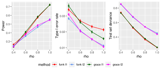
Figure 9: Simulation results for fully informative networks, comparing glm-funk and Grace estimators. Means over 100 replicates are displayed with standard error bars. Left: power, middle: Type I error rate, right: test set deviance.

Deleted true edges

We now consider the same data-generating process, where knowledge of the feature network is restricted to the inactive set of features. That is, we remove the edges connecting the $s$ active features in $G_{p}$. Note that this network is less informative than the full $G_{p}$, but not uninformative, since we do not have any false edges. We compare the same set of estimators as in the main paper. As shown in Figure 10, the glm-funk estimators perform worse, but still maintain an advantage over the lasso-based methods.

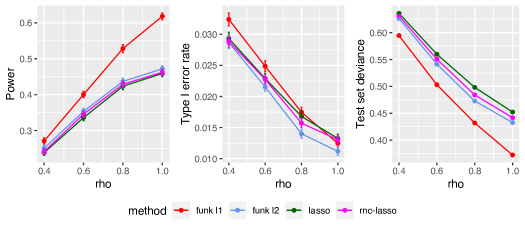
Figure 10: Simulation results for less informative networks. Means over 100 replicates are displayed with standard error bars. Left: power, middle: Type I error rate, right: test set deviance.

References

- Aitchison [1982] John Aitchison. The statistical analysis of compositional data. Journal of the Royal Statistical Society: Series B (Statistical Methodology), 44(2):139–160, 1982.
- Beck and Teboulle [2009] Amir Beck and Marc Teboulle. A fast iterative shrinkage-thresholding algorithm for linear inverse problems. SIAM journal on imaging sciences, 2(1):183–202, 2009.
- Besag [1974] Julian Besag. Spatial interaction and the statistical analysis of lattice systems. Journal of the Royal Statistical Society: Series B (Statistical Methodology), 36(2):192–225, 1974.
- Besag and Kooperberg [1995] Julian Besag and Charles Kooperberg. On conditional and intrinsic autoregressions. Biometrika, 82(4):733–746, 1995.
- Besag et al. [1991] Julian Besag, Jeremy York, and Annie Mollié. Bayesian image restoration, with two applications in spatial statistics. Annals of the Institute of Statistical Mathematics, 43(1):1–20, 1991.
- Bühlmann [2013] Peter Bühlmann. Statistical significance in high-dimensional linear models. Bernoulli, 19(4):1212–1242, 2013.
- Bühlmann and van de Geer [2011] Peter Bühlmann and Sara van de Geer. Statistics for high-dimensional data: methods, theory and applications. Springer Science & Business Media, 2011.
- Cai et al. [2019] Liqian Cai, Arnab Bhattacharjee, Roger Calantone, and Taps Maiti. Variable selection with spatially autoregressive errors: a generalized moments lasso estimator. Sankhya B, 81:146–200, 2019.
- Chen et al. [2012] Xi Chen, Qihang Lin, Seyoung Kim, Jaime G Carbonell, and Eric P Xing. Smoothing proximal gradient method for general structured sparse regression. The Annals of Applied Statistics, 6(2):719–752, 2012.
- Chernozhukov et al. [2021] Victor Chernozhukov, Wolfgang Karl Härdle, Chen Huang, and Weining Wang. LASSO-driven inference in time and space. Annals of Statistics, 49(3):1702 – 1735, 2021. doi: 10.1214/20-AOS2019. URL https://doi.org/10.1214/20-AOS2019.
- Chung [1997] Fan RK Chung. Spectral graph theory, regional conference series in math. CBMS, Amer. Math. Soc, 1997.
- Cressie [2015] Noel Cressie. Statistics for spatial data. John Wiley & Sons, 2015.
- Dean et al. [2001] CB Dean, MD Ugarte, and AF Militino. Detecting interaction between random region and fixed age effects in disease mapping. Biometrics, 57(1):197–202, 2001.
- Dezeure et al. [2015] Ruben Dezeure, Peter Bühlmann, Lukas Meier, and Nicolai Meinshausen. High-dimensional inference: Confidence intervals, p-values and r-software hdi. Statistical Science, pages 533–558, 2015.
- Duchamp and Stuetzle [2003] Tom Duchamp and Werner Stuetzle. Spline smoothing on surfaces. Journal of Computational and Graphical Statistics, 12(2):354–381, 2003.
- Guan and Haran [2018] Yawen Guan and Murali Haran. A computationally efficient projection-based approach for spatial generalized linear mixed models. Journal of Computational and Graphical Statistics, 27(4):701–714, 2018.
- Haris et al. [2019] Asad Haris, Noah Simon, and Ali Shojaie. Generalized Sparse Additive Models. arXiv e-prints, art. arXiv:1903.04641, Mar 2019.
- Hodges and Reich [2010] James S Hodges and Brian J Reich. Adding spatially-correlated errors can mess up the fixed effect you love. The American Statistician, 64(4):325–334, 2010.
- Holland et al. [1983] Paul W Holland, Kathryn Blackmond Laskey, and Samuel Leinhardt. Stochastic blockmodels: First steps. Social Networks, 5(2):109–137, 1983.
- Hughes [2015] John Hughes. copcar: A flexible regression model for areal data. Journal of Computational and Graphical Statistics, 24(3):733–755, 2015.
- Javanmard and Montanari [2013] Adel Javanmard and Andrea Montanari. Confidence intervals and hypothesis testing for high-dimensional statistical models. In Advances in Neural Information Processing Systems, pages 1187–1195, 2013.
- Lee et al. [2016] Jason D Lee, Dennis L Sun, Yuekai Sun, Jonathan E Taylor, et al. Exact post-selection inference, with application to the lasso. Annals of Statistics, 44(3):907–927, 2016.
- Leroux et al. [2000] Brian G Leroux, Xingye Lei, and Norman Breslow. Estimation of disease rates in small areas: a new mixed model for spatial dependence. In Statistical models in epidemiology, the environment, and clinical trials, pages 179–191. Springer, 2000.
- Li and Li [2008] Caiyan Li and Hongzhe Li. Network-constrained regularization and variable selection for analysis of genomic data. Bioinformatics, 24(9):1175–1182, 2008.
- Li et al. [2019] Tianxi Li, Elizaveta Levina, and Ji Zhu. Prediction models for network-linked data. The Annals of Applied Statistics, 13(1):132–164, 2019.
- Li et al. [2018] Yifeng Li, Fang-Xiang Wu, and Alioune Ngom. A review on machine learning principles for multi-view biological data integration. Briefings in Bioinformatics, 19(2):325–340, 2018.
- Lindgren and Rue [2015] Finn Lindgren and Håvard Rue. Bayesian spatial modelling with R-INLA. Journal of Statistical Software, 63(19), 2015.
- Morris et al. [2019] Mitzi Morris, Katherine Wheeler-Martin, Dan Simpson, Stephen J Mooney, Andrew Gelman, and Charles DiMaggio. Bayesian hierarchical spatial models: Implementing the besag york mollié model in stan. Spatial and Spatio-temporal Epidemiology, 31:100301, 2019.
- Negahban et al. [2012] Sahand N Negahban, Pradeep Ravikumar, Martin J Wainwright, and Bin Yu. A unified framework for high-dimensional analysis of -estimators with decomposable regularizers. Statistical Science, 27(4):538–557, 2012.
- Price-Haywood et al. [2020] Eboni G Price-Haywood, Jeffrey Burton, Daniel Fort, and Leonardo Seoane. Hospitalization and mortality among black patients and white patients with covid-19. New England Journal of Medicine, 382(26):2534–2543, 2020.
- Rabinowicz and Rosset [2022] Assaf Rabinowicz and Saharon Rosset. Cross-validation for correlated data. Journal of the American Statistical Association, 117(538):718–731, 2022.
- Randolph et al. [2018] Timothy W Randolph, Sen Zhao, Wade Copeland, Meredith Hullar, and Ali Shojaie. Kernel-penalized regression for analysis of microbiome data. The Annals of Applied Statistics, 12(1):540–566, 2018.
- Reich et al. [2006] Brian J Reich, James S Hodges, and Vesna Zadnik. Effects of residual smoothing on the posterior of the fixed effects in disease-mapping models. Biometrics, 62(4):1197–1206, 2006.
- Riebler et al. [2016] Andrea Riebler, Sigrunn H Sørbye, Daniel Simpson, and Håvard Rue. An intuitive bayesian spatial model for disease mapping that accounts for scaling. Statistical Methods in Medical Research, 25(4):1145–1165, 2016.
- Ritz and Spiegelman [2004] John Ritz and Donna Spiegelman. Equivalence of conditional and marginal regression models for clustered and longitudinal data. Statistical Methods in Medical Research, 13(4):309–323, 2004.
- Rue and Held [2005] Havard Rue and Leonhard Held. Gaussian Markov random fields: theory and applications. CRC press, 2005.
- Rue et al. [2009] Håvard Rue, Sara Martino, and Nicolas Chopin. Approximate bayesian inference for latent gaussian models by using integrated nested laplace approximations. Journal of the Royal Statistical Society: Series B (Statistical Methodology), 71(2):319–392, 2009.
- Ruppert et al. [2003] David Ruppert, Matt P Wand, and Raymond J Carroll. Semiparametric regression. Cambridge University Press, 2003.
- Sun and Zhang [2012] Tingni Sun and Cun-Hui Zhang. Scaled sparse linear regression. Biometrika, 99(4):879–898, 2012.
- Tibshirani et al. [2011] Ryan J Tibshirani, Jonathan Taylor, et al. The solution path of the generalized lasso. Annals of Statistics, 39(3):1335–1371, 2011.
- van de Geer [2000] Sara van de Geer. Empirical Processes in M-estimation, volume 6. Cambridge University Press, 2000.
- van de Geer et al. [2014] Sara van de Geer, Peter Bühlmann, Ya’acov Ritov, and Ruben Dezeure. On asymptotically optimal confidence regions and tests for high-dimensional models. Annals of Statistics, 42(3):1166–1202, 2014.
- Vershynin [2018] Roman Vershynin. High-dimensional probability: An introduction with applications in data science, volume 47. Cambridge University Press, 2018.
- Wahba [1981] Grace Wahba. Spline interpolation and smoothing on the sphere. SIAM Journal on Scientific and Statistical Computing, 2(1):5–16, 1981.
- Wainwright [2019] Martin J Wainwright. High-dimensional statistics: A non-asymptotic viewpoint, volume 48. Cambridge University Press, 2019.
- Wang et al. [2016] Yu-Xiang Wang, James Sharpnack, Alexander J Smola, and Ryan J Tibshirani. Trend filtering on graphs. The Journal of Machine Learning Research, 17(1):3651–3691, 2016.
- Wasserman and Roeder [2009] Larry Wasserman and Kathryn Roeder. High dimensional variable selection. Annals of Statistics, 37(5A):2178, 2009.
- Wright [2015] Stephen J Wright. Coordinate descent algorithms. Mathematical Programming, 151(1):3–34, 2015.
- Zhang and Zhang [2014] Cun-Hui Zhang and Stephanie S Zhang. Confidence intervals for low dimensional parameters in high dimensional linear models. Journal of the Royal Statistical Society: Series B (Statistical Methodology), 76(1):217–242, 2014.
- Zhao and Shojaie [2016] Sen Zhao and Ali Shojaie. A significance test for graph-constrained estimation. Biometrics, 72(2):484–493, 2016.