Sample Complexity of the Sign-Perturbed Sums Identification Method: Scalar Case

Abstract

Sign-Perturbed Sum (SPS) is a powerful finite-sample system identification algorithm which can construct confidence regions for the true data generating system with exact coverage probabilities, for any finite sample size. SPS was developed in a series of papers and it has a wide range of applications, from general linear systems, even in a closed-loop setup, to nonlinear and nonparametric approaches. Although several theoretical properties of SPS were proven in the literature, the sample complexity of the method was not analysed so far. This paper aims to fill this gap and provides the first results on the sample complexity of SPS. Here, we focus on scalar linear regression problems, that is we study the behaviour of SPS confidence intervals. We provide high probability upper bounds, under three different sets of assumptions, showing that the sizes of SPS confidence intervals shrink at a geometric rate around the true parameter, if the observation noises are subgaussian. We also show that similar bounds hold for the previously proposed outer approximation of the confidence region. Finally, we present simulation experiments comparing the theoretical and the empirical convergence rates.

1 Introduction

Estimating models is a fundamental problem across several domains, such as system identification, machine learning and statistics. System identification, a research area that studies how to build models of dynamical systems from observed data, has a long and rich history. Classical methods in the field provide asymptotically guaranteed estimates and confidence regions (Söderström and Stoica, 1989; Ljung, 1999). Recently, a paradigm shift took place in the field and more significant emphasis was given to approaches with non-asymptotic guarantees. Most of these techniques assume that the noises and disturbances follow given (known) distributions, therefore distribution-free, non-asymptotic identification of dynamical systems still remain an active area of research (Carè et al., 2018).

Two promising identification algorithms that can construct non-asymptotic confidence regions around the true parameter, for any finite sample, in a distribution-free setting are the LSCR: Leave-out Sign-dominant Correlation Regions (Campi and Weyer, 2005) and the SPS: Sign-Perturbed Sums (Csáji et al., 2015) methods.

SPS constructs exact confidence regions around the least-squares estimate for any finite sample, under mild assumptions on the noises, namely that they are independent and their probability distributions are symmetric about zero.

Several important properties of SPS, such as its exact coverage probability (Csáji et al., 2015) and strong consistency (Weyer et al., 2017), were rigorously proven for linear regression problems, under the assumptions mentioned above. The standard SPS method provides an indicator function, which evaluates whether a given parameter is included in the confidence region. In (Csáji et al., 2015) an ellipsoidal outer approximation algorithm was proposed that builds a compact representation of the confidence set around the least-squares estimate. The symmetricity assumption on the noises was relaxed in (Kolumbán et al., 2015). The closed-loop applicability of SPS was studied in (Csáji and Weyer, 2015), and in (Volpe et al., 2015) an instrumental variable based generalization was given that can construct confidence regions for ARX systems with the same theoretical guarantees as mentioned before. The behaviour of SPS was also investigated in the face of undermodelling (Carè et al., 2021). Further extensions and applications of SPS include kernel-based methods (Csáji and Kis, 2019; Baggio et al., 2022), nonparametric confidence bands (Csáji and Horváth, 2022) and even tests for binary classification (Tamás and Csáji, 2021).

Although the confidence regions generated by SPS are strongly consistent, the sample complexity of the method remained an open question. Here, we give distribution-free, high probability bounds for the length of SPS confidence intervals for any finite sample size. As a first line of sample complexity research for SPS, the emphasis of our study is on the possible tools of theoretical analysis, hence, we restrict our attention to the scalar-valued case. Although we only investigate the scalar setting, the obtained results are directly relevant, for example, for multi-armed bandit problems (Lattimore and Szepesvári, 2020), prediction intervals, confidence bands (Csáji and Horváth, 2022) and signal processing approaches (Csáji and Weyer, 2011).

Our main contributions in this paper are as follows:

1. Non-asymptotic analysis of SPS in case of the “constant in noise” setting, assuming subgaussian noises.

2. High probability upper bounds for the sizes of SPS confidence intervals for scalar linear regression, both for deterministic and stochastic regressors.

3. Simulation experiments to compare the obtained theoretical bounds with the empirical performance.

The paper is structured as follows. In Section 2 we give a short overview of SPS and its fundamental properties. Section 3 provides our theoretical non-asymptotic results on the size of the SPS confidence regions with proofs. The simulation experiments are presented in Section 4. Finally, Section 5 summarizes and concludes the paper.

2 The Sign-Perturbed Sums algorithm

In this section we give an overview of SPS for scalar linear regression. The reader is referred to (Csáji et al., 2015) and (Weyer et al., 2017) for a detailed description of the algorithm in the general (d-dimensional) linear regression case, with theorems and proofs. Note that in our study we discard (w.l.o.g.) the “shaping matrix” term of the algorithm, since its purpose is take the inter-dependencies of the parameteres into account, in case $d>1$. In the scalar case this does not affect the constructed intervals.

2.1 Problem setting and main assumptions

Consider the following scalar linear regression system

$$y_{t}=\varphi_{t}\hskip 0.85358pt\theta^{*}+w_{t},\vspace{1mm}$$ (1)

where $\varphi_{t}\in\mathbb{R}$ is the regressor, $y_{t}\in\mathbb{R}$ is the output, $w_{t}\in\mathbb{R}$ is the noise and $\theta^{*}\in\mathbb{R}$ is the (constant) “true” parameter to be estimated. We are given a sample of size $n$ which consists of $\varphi_{1},\dots,\varphi_{n}$ (inputs) and $y_{1},\dots,y_{n}$ (outputs).

The assumptions on the noises and the regressors are

• $\{w_{t}\}$ is a sequence of independent random variables and each $w_{t}$ has a symmetric probability distribution about zero (i.e., $w_{t}$ has the same distribution as $-w_{t}$).
  

• The regressors, $\{\varphi_{t}\}$, are almost surely nonzero random variables, and $\{\varphi_{t}\}$ is independent of $\{w_{t}\}$.

2.2 The SPS algorithm and its theoretical properties

In linear regression problems given a sample of size $n$ the least-squares estimate (LSE) can be obtained by solving the normal equation. The core idea behind SPS is to introduce $m-1$ sign-perturbed sums $\{S_{i}(\theta)\}$ and a reference sum $S_{0}(\theta)$ from the normal equation and construct a confidence region based on the rank of $S_{0}(\theta)$.

The SPS algorithm consists of two parts, an initialization phase and an indicator function. In the initialization part the algorithm calculates the main parameters and generates the random signs needed for the construction of the confidence region. The indicator function evaluates whether a given parameter $\theta$ is included in the confidence interval. The initialization is shown in Table 1 and the indicator is presented in Table 2.

Table 1: Pseudocode: SPS-Initialization $(\hskip 0.56905ptp\hskip 0.56905pt)$

1.	Given a (rational) confidence probability $p\in(0,1)$, set integers $m>q>0$ such that $p=1-q/m$;
2.	Generate $n(m-1)$ i.i.d random signs $\{\alpha_{i,t}\}$ with $$\mathbb{P}(\alpha_{i,t}=1)=\,\mathbb{P}(\alpha_{i,t}=-1)=0.5$$ for all integers $1\leq i\leq m-1$ and $1\leq t\leq n$.
3.	Generate a permutation $\pi$ of the set $\{0,\dots,m-1\}$ randomly, where each of the $m!$ possible permutations has the same probability $1/(m!)$ to be selected.

Table 2: Pseudocode: SPS-Indicator $(\hskip 0.56905pt\theta\hskip 0.56905pt)$

1.	For a given $\theta$, compute the prediction errors $$\varepsilon_{t}(\theta)\doteq y_{t}-\varphi_{t}\theta\vspace{-1mm}$$ for all $1\leq t\leq n$;
2.	Evaluate $$S_{0}(\theta)\doteq\sum_{t=1}^{n}\varphi_{t}\varepsilon_{t}(\theta),\quad\text{and}\quad S_{i}(\theta)\doteq\sum_{t=1}^{n}\alpha_{i,t}\varphi_{t}\varepsilon_{t}(\theta),\vspace{-0.5mm}$$ for all indices $1\leq i\leq m-1$;
3.	Order scalars $\{S_{i}^{2}(\theta)\}$ according to $\succ_{\pi}$, where “$\succ_{\pi}$” is “$>$” with random tie-breaking (Csáji et al., 2015);
4.	Compute the rank $\mathcal{R}(\theta)$ of $S_{0}^{2}(\theta)$ in the ordering where $$\mathcal{R}(\theta)\doteq\Bigg{[}1+\sum_{i=1}^{m-1}\mathbb{I}\left(S_{0}^{2}(\theta)\succ_{\pi}S_{i}^{2}(\theta)\right)\Bigg{]};\vspace{-2mm}$$
5.	Return 1 if $\mathcal{R}(\theta)\leq m-q$, otherwise return 0.

Using this construction, the $p$-level SPS confidence region can be defined as

$$\mathcal{C}_{p}\,\doteq\,\{\,\theta\in\mathbb{R}\text{ : SPS-Indicator}(\theta)=1\,\}.\vspace{1mm}$$ (2)

As it was shown for general linear regression problems in (Csáji et al., 2015), the confidence region $\mathcal{C}_{p}$ contains the true parameter $\theta^{*}$ exactly with probability $p$, thus

Theorem 1

Assuming A1 and A2, the coverage probability of the SPS confidence interval is exactly $p$, that is,

$$\mathbb{P}(\theta^{*}\in\mathcal{C}_{p})\,=\,1-\frac{q}{m}\,=\,p.\vspace{-1mm}$$ (3)

Note that in (Csáji et al., 2015) this theorem is proved for deterministic regressors, but it is straightforward to generalize the result to the case of random regressors that are independent of the noises (i.e., by conditioning on the regressors, as the deterministic result can be applied to almost all realizations of the regressors). In (Weyer et al., 2017) it has been rigorously proved that the confidence regions are also strongly consistent, which requires some further mild assumptions that we do not detail here.

To give a compact representation of the confidence region around the LSE, an ellipsoidal outer approximation method was developed (Csáji et al., 2015). The confidence interval given by the outer approximation in our case is

$$\mathcal{C}_{p}\,\subseteq\,\mathcal{O}_{p}\,\doteq\,\big{\{}\,\theta\in\mathbb{R}:(\theta-\hat{\theta}_{n})^{2}r_{n}\leq r\,\big{\}},\vspace{1mm}$$ (4)

where $r_{n}=\tfrac{1}{n}\sum_{t=1}^{n}\varphi_{t}^{2}$ and $r$ can be calculated from the (ordering of the) solutions of the following optimization problems, for all $0<i<m$, (Csáji et al., 2015)

maximize $$S_{0}^{2}(\theta)$$ (5)

subject to $$S_{0}^{2}(\theta)-S_{i}^{2}(\theta)\leq 0.$$

An illustrative example of the scalar SPS confidence regions for $m=2$ and $\forall\,t:\varphi_{t}=1$, is presented in Fig.  1. The confidence region consists of the points $\{\theta\in\mathbb{R}:S_{0}^{2}(\theta)\leq S_{1}^{2}(\theta)\}$. In the case of outer approximation, from (5) we have $\sqrt{r}=\max(|\theta_{1}-\hat{\theta}_{n}|,|\theta_{2}-\hat{\theta}_{n}|)$, hence, the outer approximation is given by $\{\theta\in\mathbb{R}:|\theta-\hat{\theta}_{n}|\leq\sqrt{r}\}$.

In case of a scalar parameter, the SPS confidence regions are in fact intervals. Thus, they automatically have nice representations, hence their outer approximations look superfluous (unlike in higher dimensions). Nevertheless, we also study the behaviour of the outer approximations, since we want to understand their sample complexity, as well, as they are very important for multi-dimensional settings.

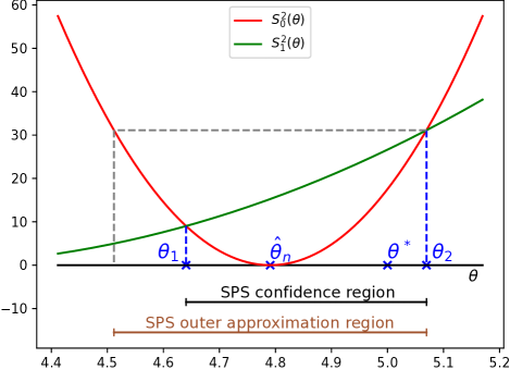
Figure 1: SPS confidence intervals, $m=2$ ($50\,\%$ confidence).

3 Sample complexity of SPS

In this section we prove high probability upper bounds for the lengths of SPS confidence intervals. We analyze SPS assuming a one-dimensional constant parameter, first without inputs. Then, we investigate linear regression with scalar inputs, using two other sets of assumptions.

3.1 Identifying a “constant in noise”

Consider the problem of identifying a constant in noise

$$y_{t}=\theta^{*}+w_{t},\vspace{0.5mm}$$ (6)

for $t=1,\dots,n$, where $y_{t}$ is the output, $w_{t}$ is the noise and $\theta^{*}$ is the true parameter (constant). Both the random variables $y_{t}$, $w_{t}$ and the optimal parameter $\theta^{*}$ are scalars.

For this analysis, we also assume that

• Every noise term, $w_{t}$, has a nonatomic, subgaussian distribution with variance proxy $\sigma^{2}$, that is $\forall\,\lambda\in\mathbb{R}:$

  $$\mathbb{E}\big{[}\exp(\lambda w_{t})\hskip 0.85358pt\big{]}\,\leq\,\exp\!{\left(\frac{\lambda^{2}\sigma^{2}}{2}\right)}.$$ (7)

Note that this assumption is much weaker than assuming Gaussian noises. For example, every distribution with bounded support is automatically subgaussian, therefore, it covers a wide range of possible noises. The nonatomicity of the distributions is nonessential, it is only used to avoid ties and, thus, to simplify the analysis. Moreover, SPS does not exploit subgaussianity in any way, A3 is used solely for the sake of studying the sample complexity of SPS.

Carè (2022) has shown that the SPS confidence regions are bounded, if both the perturbed and the unperturbed regressors span the whole space. In our current setting, this means that there should be at least one positive and one negative sign in each sign-perturbation sequence. Thus, in order to guarantee boundedness, we assume

• For all  $0<i<m$, we have $\alpha_{i,1}=1$ and $\alpha_{i,2}=-1$.

Before we state our theorem, we first prove a lemma that is an essential part of the proof of the later theorem.

Lemma 2

Assume A1 and A3, $n>2$, and let

$$X_{+}\doteq\frac{\sum_{t=1}^{n}(1+\alpha_{t})w_{t}}{\sum_{t=1}^{n}(1+\alpha_{t})},\qquad X_{-}\doteq\frac{\sum_{t=1}^{n}(1-\alpha_{t})w_{t}}{\sum_{t=1}^{n}(1-\alpha_{t})},\vspace{1mm}$$

where $\alpha_{1}=1$, $\alpha_{2}=-1$, and $\{\alpha_{t}\}_{t=3}^{n}$ are i.i.d. Rademacher random variables, independent of the noise terms $\{w_{t}\}$.

Then, variables $X_{+}$ and $X_{-}$ satisfy for all $\varepsilon\geq 0:$

$$\mathbb{P}\left(|X_{\pm}|\geq\varepsilon\right)\,\leq\,2\left(\frac{1}{2}+\frac{1}{2}\exp\left(-\frac{\varepsilon^{2}}{2\sigma^{2}}\right)\right)^{\!n-1}.\vspace{-2mm}$$ (8)

Observe that $\sum_{t=1}^{n}(1-\alpha_{t})\overset{d}{=}\sum_{t=1}^{n}(1+\alpha_{t})$, therefore it is enough to prove the claim for $X_{+}$, which in this proof we will denote by $X$ for shorthand of notation.

Let $Z=\sum_{t=3}^{n}(1+\alpha_{t})/2$, which has a binomial distribution with parameters $(1/2,n-2)$. By using the law of total probability, the following can be written

$$\mathbb{P}\left(|X|\geq\varepsilon\right)\,=\,\mathbb{P}\left(\Bigg{|}\,\frac{\sum_{t=1}^{n}(1+\alpha_{t})w_{t}}{\sum_{t=1}^{n}(1+\alpha_{t})}\,\Bigg{|}\geq\varepsilon\right)\,=\,$$

$$\sum_{k=0}^{n-2}\mathbb{P}\left(\Bigg{|}\,\frac{\tfrac{1}{2}\sum_{t=1}^{n}(1+\alpha_{t})w_{t}}{\tfrac{1}{2}\sum_{t=1}^{n}(1+\alpha_{t})}\,\Bigg{|}\geq\varepsilon\,\bigg{|}\,Z=k\right)\mathbb{P}(Z=k)$$

$$=\sum_{k=0}^{n-2}\mathbb{P}\left(\Bigg{|}\,\frac{\sum_{t\in I_{k+1}}w_{t}}{k+1}\,\Bigg{|}\geq\varepsilon\right)\mathbb{P}(Z=k),$$ (9)

where $I_{k+1}$ is a random index set of length $k+1$. Note, that the index sets of length $k+1$ are uniformly distributed, since every one of them has the same probability, $1/2^{n-2}$. For every (finitely many) realization of $I_{k+1}$, the variance proxy of $(\sum_{t\in I_{k+1}}w_{t})/(k+1)$ is always $\sigma\sqrt{1/(k+1)}$, which follows from the properties of subgaussian variables (Lattimore and Szepesvári, 2020, Lemma 5.4). Then, the above probability (3.1) can be upper bounded by using the Hoeffding inequality (Wainwright, 2019, Proposition 2.5)

$$\leq\,2\sum_{k=0}^{n-2}\mathbb{P}(Z=k)\exp\!\left(-\frac{(k+1)\varepsilon^{2}}{2\sigma^{2}}\right)$$

$$=\,2\;\mathbb{E}\!\left[\exp\!\left(-\frac{Z\varepsilon^{2}}{2\sigma^{2}}\right)\right]\exp\!\left(-\frac{\varepsilon^{2}}{2\sigma^{2}}\right)$$

$$=\,2\left(\frac{1}{2}+\frac{1}{2}\exp\left(-\frac{\varepsilon^{2}}{2\sigma^{2}}\right)\right)^{\!n-2}\!\exp\!\left(-\frac{\varepsilon^{2}}{2\sigma^{2}}\right)$$

$$\leq\,2\left(\frac{1}{2}+\frac{1}{2}\exp\left(-\frac{\varepsilon^{2}}{2\sigma^{2}}\right)\right)^{\!n-1},$$

where we applied the moment generating function of the binomial distribution, to express $\mathbb{E}[\hskip 0.85358pt\exp(t\hskip 0.85358ptZ)\hskip 0.85358pt]$. $\square$

Now, we state our nonasymptotic high probability upper bound for the length of SPS confidence intervals.

Theorem 3

Assuming A1, A3, A4, and considering system (6), the confidence intervals generated by SPS are shrinking at a geometric rate, i.e., for all $\varepsilon>0$,

$$\mathbb{P}\Big{(}\sup_{\theta\in\mathcal{C}_{p}}\left\lvert\hskip 0.85358pt\theta-\theta^{*}\right\rvert\geq\varepsilon\Big{)}\leq$$

$$4\,\hskip 0.85358pt(m-q)\left(\frac{1}{2}+\frac{1}{2}\exp\left(-\frac{\varepsilon^{2}}{2\sigma^{2}}\right)\right)^{\!n-1}.$$ (10)

First, we derive the sample complexity of SPS for the case where there are only two sums $S_{0}(\theta)$ and $S_{1}(\theta)$, and later generalize this to the case, where there are $m$ sums. In the case of two sums, $S_{0}(\theta)$ and $S_{1}(\theta)$ are:

$$S_{0}(\theta) \,=\,n(\theta^{*}-\theta)+w,$$ (11)

$$S_{1}(\theta) \,=\,\alpha(\theta^{*}-\theta)+w_{\alpha},\vspace{1mm}$$ (12)

where $n$ is the sample size, $w\doteq\sum_{t=1}^{n}w_{t}$, $\alpha\doteq\sum_{t=1}^{n}\alpha_{t}$ and $w_{\alpha}\doteq\sum_{t=1}^{n}\alpha_{t}w_{t}$. Then, a $p=0.5$ confidence set is

$$\mathcal{C}_{0.5}=\{\,\theta:S_{0}^{2}(\theta)\leq S_{1}^{2}(\theta)\,\}=\{\,\theta:\theta_{1}\leq\theta\leq\theta_{2}\,\},\vspace{1mm}$$ (13)

where $\theta_{1}$ and $\theta_{2}$ are the intersections of the two parabolas determined by $S_{0}^{2}(\theta)$ and $S_{1}^{2}(\theta)$. If the confidence region is finite, then $\theta_{1}$ and $\theta_{2}$ always exist. The pair $\theta_{1}$ and $\theta_{2}$ can be calculated by solving the quadratic equation

$$S_{0}^{2}(\theta)-S_{1}^{2}(\theta)=a^{2}\theta^{2}+2b\theta+c=0,\vspace{1mm}$$ (14)

where $a=(n^{2}-\alpha^{2})$, $b=(\alpha^{2}-n^{2})\theta^{*}+\alpha w_{\alpha}-nw$ and $c=(\theta^{*})^{2}(n^{2}-\alpha^{2})+2\theta^{*}(nw-\alpha w_{\alpha})+w^{2}-w_{\alpha}^{2}$. The solutions are

$$\theta_{1}=\dfrac{w+w_{\alpha}+\alpha\theta^{*}+n\theta^{*}}{\alpha+n}=\dfrac{w+w_{\alpha}}{\alpha+n}+\theta^{*}=$$

$$\dfrac{\sum_{t=1}^{n}w_{t}(1+\alpha_{t})}{\sum_{t=1}^{n}(1+\alpha_{t})}+\theta^{*}\!\!,$$ (15)

$$\theta_{2}=\dfrac{-w+w_{\alpha}+\alpha\theta^{*}-n\theta^{*}}{\alpha-n}=\dfrac{w-w_{\alpha}}{n-\alpha}+\theta^{*}=$$

$$\dfrac{\sum_{t=1}^{n}w_{t}(1-\alpha_{t})}{\sum_{t=1}^{n}(1-\alpha_{t})}+\theta^{*}\!\!.$$ (16)

Throughout our analysis we give concentration inequalities for the quantities $\left\lvert\hskip 0.85358pt\theta_{1}-\mathbb{E}[\theta_{1}]\right\rvert$ and $\lvert\hskip 0.85358pt\theta_{2}-\mathbb{E}[\theta_{2}]\rvert$. The sequences $\{w_{t}\}$ and $\{\alpha_{t}\}$ are independent, and $\{w_{t}\}$ is centered, thus $\mathbb{E}[\theta_{1}]=\mathbb{E}[\theta_{2}]=\theta^{*}$. Using the results from Lemma 2, it holds for for $j=1,2$ and any $\varepsilon>0$ that

$$\mathbb{P}(\left\lvert\hskip 0.85358pt\theta_{j}-\theta^{*}\right\rvert\geq\varepsilon)\,\leq\,2\left(\frac{1}{2}+\frac{1}{2}\exp\left(-\frac{\varepsilon^{2}}{2\sigma^{2}}\right)\right)^{\!n-1}.$$ (17)

Then, using the union bound (Boole’s inequality), we have

$$\mathbb{P}\Big{(}\sup_{\theta\in\mathcal{C}_{0.5}}\left\lvert\hskip 0.85358pt\theta-\theta^{*}\right\rvert\geq\varepsilon\Big{)}=\,\mathbb{P}\Big{(}\max_{j=1,2}\left\lvert\hskip 0.85358pt\theta_{j}-\theta^{*}\right\rvert\geq\varepsilon\Big{)}\,\leq$$

$$4\left(\frac{1}{2}+\frac{1}{2}\exp\left(-\frac{\varepsilon^{2}}{2\sigma^{2}}\right)\right)^{\!n-1},\vspace{1mm}$$ (18)

for all $\varepsilon>0$. Note that (18) only holds for the special case of $m=2$ and $q=1$ (i.e., confidence probability $0.5$).

Now, we consider the general case, i.e., we allow arbitrary $0<q<m$ (integer) choices. Our aim will be to provide an upper bound for the probability of the “bad” event that the length of the constructed interval is above a given $\varepsilon>0$. First, we can construct bad events for each $i$, i.e., the event that the $0.5$ probability interval defined by $S_{0}(\theta)$ and $S_{i}(\theta)$, cf. (13), has length at least $\varepsilon$. This event is

$$B_{i}^{\hskip 0.85358pt\varepsilon}\,\doteq\,\big{\{}\,\omega\in\Omega:\max_{j=1,2}\left\lvert\hskip 0.85358pt\theta_{i,j}(\omega)-\theta^{*}\right\rvert\geq\varepsilon\,\big{\}},\vspace{1mm}$$ (19)

where $\theta_{i,1}$ and $\theta_{i,2}$ are the two intersections of parabolas $S^{2}_{0}(\theta)$ and $S^{2}_{i}(\theta)$; and $\Omega$ is the sample space of the underlying probability space $(\Omega,\mathcal{F},\mathbb{P})$. We already provided an upper bound for $\mathbb{P}(B_{i}^{\hskip 0.85358pt\varepsilon})$, see (18), which is valid for all $i=1,\dots,m-1$; but $B_{1}^{\hskip 0.85358pt\varepsilon},\dots,B_{m-1}^{\hskip 0.85358pt\varepsilon}$ are not independent.

By using the construction of SPS, see (Csáji et al., 2015), the “good” event, given integers $0<q<m$, is

$$G^{\hskip 0.85358pt\varepsilon}\,\doteq\bigcup_{\begin{subarray}{c}I\subseteq\mathcal{M},\\ |I|\geq m-q\end{subarray}}\bigcap_{i\in I}\,G_{i}^{\hskip 0.85358pt\varepsilon},$$ (20)

where $\mathcal{M}\doteq\{1,\dots,m-1\}$ and $G_{i}^{\hskip 0.85358pt\varepsilon}=\Omega\setminus B_{i}^{\hskip 0.85358pt\varepsilon}$, for $i\in\mathcal{M}$.

This means that there exist at least $m-q$ (perturbed) parabolas, $\{S^{2}_{i}\}_{i\neq 0}$, such that all of their intersections with the reference $S^{2}_{0}$ are closer to $\theta^{*}$ than the given $\varepsilon>0$.

Then, by using De Morgan’s laws, the “bad” event is

$$B^{\hskip 0.85358pt\varepsilon}\,\doteq\;\Omega\setminus G^{\hskip 0.85358pt\varepsilon}\,=\bigcap_{\begin{subarray}{c}I\subseteq\mathcal{M},\\ |I|\geq m-q\end{subarray}}\bigcup_{i\in I}\,B_{i}^{\hskip 0.85358pt\varepsilon}\,=\bigcap_{\begin{subarray}{c}I\subseteq\mathcal{M},\\ |I|=m-q\end{subarray}}\bigcup_{i\in I}\,B_{i}^{\hskip 0.85358pt\varepsilon}.\vspace{-2mm}$$ (21)

The probability of this “bad” event can be bounded by

$$\mathbb{P}(B^{\hskip 0.85358pt\varepsilon})\,\leq\min_{\begin{subarray}{c}I\subseteq\mathcal{M},\\ |I|=m-q\end{subarray}}\mathbb{P}\!\left[\,\bigcup_{i\in I}\,B_{i}^{\hskip 0.85358pt\varepsilon}\right]\,\leq\,(m-q)\cdot\mathbb{P}(B_{1}^{\hskip 0.85358pt\varepsilon}),$$ (22)

where we used that $\mathbb{P}(A\cap B)\leq\min\{\mathbb{P}(A),\,\mathbb{P}(B)\}$ and $\mathbb{P}(A\cup B)\leq\mathbb{P}(A)+\mathbb{P}(B)$. This completes the proof. $\square$

Next, we give a high probability bound on the size of the outer approximation of the SPS confidence interval.

Corollary 4

Assuming A1, A3 and A4, and considering (6), the confidence region of the SPS outer approximation is shrinking at a geometric rate, i.e., for all $\varepsilon>0$,

$$\mathbb{P}\Big{(}\sup_{\theta\in\mathcal{O}_{p}}|\hskip 0.85358pt\theta-\hat{\theta}_{n}|\geq\varepsilon\Big{)}\,\leq\,$$

$$4\,\hskip 0.85358pt(m-q)\left(\frac{1}{2}+\frac{1}{2}\exp\left(-\frac{\varepsilon^{2}}{8\sigma^{2}}\right)\right)^{\!n-1}.$$ (23)

The proof of this corollary is similar to the proof of Theorem 3, we first consider the case for two sums: $S_{0}(\theta)$ and $S_{1}(\theta)$, and then generalize it to arbitrary $0<q<m$ choices. For two sums the size of the SPS confidence region induced outer approximation is $2\max(|\hskip 0.85358pt\theta_{1}-\hat{\theta}_{n}|,|\hskip 0.85358pt\theta_{2}-\hat{\theta}_{n}|)$, therefore, we should study $\theta_{1}-\hat{\theta}_{n}$.

$$\theta_{1}-\hat{\theta}_{n}=\dfrac{\sum_{t=1}^{n}w_{t}(1+\alpha_{t})}{\sum_{t=1}^{n}(1+\alpha_{t})}+\theta^{*}-\theta^{*}-\dfrac{\sum_{t=1}^{n}w_{t}}{n}$$

$$\overset{d}{=}\;\dfrac{\sum_{t=1}^{n}w_{t}(1+\alpha_{t})}{\sum_{t=1}^{n}(1+\alpha_{t})}+\dfrac{\sum_{t=1}^{n}w_{t}}{n}.$$ (24)

By introducing $Z=\sum_{t=3}^{n}(1+\alpha_{t})/2$ and using the same ideas and notations as in the proof of Lemma 2, we have

$$\mathbb{P}\left(\Bigg{|}\,\frac{\sum_{t=1}^{n}w_{t}(1+\alpha_{t})}{\sum_{t=1}^{n}(1+\alpha_{t})}+\frac{\sum_{t=1}^{n}w_{t}}{n}\,\Bigg{|}\geq\varepsilon\right)=$$

$$\sum_{k=0}^{n-2}\mathbb{P}\left(\Bigg{|}\,\frac{\tfrac{1}{2}\sum_{t=1}^{n}w_{t}(1+\alpha_{t})}{\tfrac{1}{2}\sum_{t=1}^{n}(1+\alpha_{t})}+\frac{\sum_{t=1}^{n}w_{t}}{n}\,\Bigg{|}\geq\varepsilon\,\bigg{|}\,Z=k\right)$$

$$\cdot\mathbb{P}(Z=k)=\sum_{k=0}^{n-2}\mathbb{P}\Bigg{(}\Bigg{|}\,\sum_{t\in I_{k+1}}w_{t}\,\left(\frac{1}{k+1}+\frac{1}{n}\right)+$$

$$\frac{1}{n}\sum_{t\notin I_{k+1}}w_{t}\,\Bigg{|}\geq\varepsilon\Bigg{)}\mathbb{P}(Z=k)\leq 2\sum_{k=0}^{n-2}\mathbb{P}(Z=k)$$

$$\cdot\exp\left(\frac{-\varepsilon^{2}}{2\sigma^{2}\left[(k+1)\left(\frac{1}{k+1}+\frac{1}{n}\right)^{2}+(n-k-1)\left(\frac{1}{n}\right)^{2}\right]}\right)$$

$$=2\sum_{k=0}^{n-2}\mathbb{P}(Z=k)\exp\left(-\frac{\varepsilon^{2}}{2\sigma^{2}\left(\frac{1}{k+1}+\frac{3}{n}\right)}\right)$$

$$=2\sum_{k=0}^{n-2}\mathbb{P}(Z=k)\exp\left(-\frac{\varepsilon^{2}n(k+1)}{2\sigma^{2}\left(n+3(k+1)\right)}\right)$$

$$\,\leq\,2\sum_{k=0}^{n-2}\mathbb{P}(Z=k)\exp\left(-\frac{\varepsilon^{2}(k+1)}{8\sigma^{2}}\right)$$

$$\,\leq\,2\left(\frac{1}{2}+\frac{1}{2}\exp\left(-\frac{\varepsilon^{2}}{8\sigma^{2}}\right)\right)^{\!n-1},$$ (25)

where we also expoited that for every (finitely many) realization of $I_{k+1}$ the sum $\sum_{t\in I_{k+1}}w_{t}\,\left(1/(k+1)+1/n\right)+(1/n)\sum_{t\notin I_{k+1}}w_{t}$ has a (common) variance proxy

$$\sigma\left[(k+1)\left(\frac{1}{k+1}+\frac{1}{n}\right)^{2}+(n-k-1)\left(\frac{1}{n}\right)^{2}\right]^{1/2}.$$

Then, using the union bound

$$\mathbb{P}\Big{(}\max_{j=1,2}\left\lvert\hskip 0.85358pt\theta_{j}-\hat{\theta}_{n}\right\rvert\geq\varepsilon\Big{)}\leq\,4\left(\frac{1}{2}+\frac{1}{2}\exp\left(-\frac{\varepsilon^{2}}{8\sigma^{2}}\right)\right)^{n-1}.$$

Finally, the above result, which assumed $m=2$ and $q=1$, can be generalized to arbitrary choices of $0<q<m$ in the same way as we did in the proof of Theorem 3. $\square$

3.2 Scalar linear regression with bounded regressors

Consider the following scalar linear regression problem

$$y_{t}=\varphi_{t}\hskip 0.85358pt\theta^{*}+w_{t},\vspace{1mm}$$ (26)

where $\varphi_{t}$ the regressor, $y_{t}$ is the output, $w_{t}$ is the noise and $\theta^{*}$ is the true parameter to be estimated. Both the random variables $\varphi_{t}$, $y_{t}$, $w_{t}$, and the true parameter $\theta^{*}$ are scalars. Our assumption on the noise is still A3, and we make the following assumption on the regressors:

• The regressor sequence, $\{\varphi_{t}\}$, consists of independent random variables that are almost surely bounded from below: for all $t$, we (a.s.) have $0<\varphi_{\text{min}}\leq\left\lvert\hskip 0.85358pt\varphi_{t}\right\rvert$.

Similarly to the previous identification case, we first state and prove a lemma, then two concentration inequalities regarding the size of the confidence region generated by the SPS algorithm and its outer approximation.

Lemma 5

Assume A1, A2, A3 and A5, $n>2$, and let

$$X_{1,2}\doteq\frac{\sum_{t=1}^{n}\varphi_{t}(1\pm\alpha_{t})w_{t}}{\sum_{t=1}^{n}\varphi_{t}^{2}(1\pm\alpha_{t})}$$

where $\alpha_{1}=1$, $\alpha_{2}=-1$, and $\{\alpha_{t}\}_{t=3}^{n}$ are i.i.d. Rademacher random variables, independent of the noise terms $\{w_{t}\}$.

Then, variables $X_{1}$ and $X_{2}$ satisfy for all $\varepsilon\geq 0:$

$$\mathbb{P}\left(|X_{1,2}|\geq\varepsilon\right)\,\leq\,2\left(\frac{1}{2}+\frac{1}{2}\exp\left(-\frac{\varepsilon^{2}\varphi_{\text{min}}^{2}}{2\sigma^{2}}\right)\right)^{\!n-1}.\vspace{-2mm}$$ (27)

Note that as $X_{1}\overset{d}{=}X_{2}$, it is enough to prove the claim for $X_{1}$. Then, by introducing $Z=\sum_{t=3}^{n}(1+\alpha_{t})/2$ and using the same arguments and notations as in the proof of Lemma 2, an overbound can be calulated as

$$\mathbb{P}\left(|X_{1}|\geq\varepsilon\right)\,=\,\mathbb{P}\left(\Bigg{|}\,\frac{\sum_{t=1}^{n}\varphi_{t}(1+\alpha_{t})w_{t}}{\sum_{t=1}^{n}\varphi_{t}^{2}(1+\alpha_{t})}\,\Bigg{|}\geq\varepsilon\right)\,=$$

$$\sum_{k=0}^{n-2}\mathbb{P}\left(\Bigg{|}\,\frac{\tfrac{1}{2}\sum_{t=1}^{n}\varphi_{t}(1+\alpha_{t})w_{t}}{\tfrac{1}{2}\sum_{t=1}^{n}\varphi_{t}^{2}(1+\alpha_{t})}\,\Bigg{|}\geq\varepsilon\,\bigg{|}\,Z=k\right)\mathbb{P}(Z=k)$$

$$=\sum_{k=0}^{n-2}\mathbb{P}\left(\Bigg{|}\,\frac{\sum_{t\in I_{k+1}}\varphi_{t}w_{t}}{\sum_{t\in I_{k+1}}\varphi_{t}^{2}}\Bigg{|}\geq\varepsilon\right)\mathbb{P}(Z=k)$$

$$\,\leq\,2\sum_{k=0}^{n-2}\mathbb{P}(Z=k)\exp\!\left(-\frac{\varepsilon^{2}(k+1)\varphi_{\text{min}}^{2}}{2\sigma^{2}}\right)$$

$$\,\leq\,2\left(\frac{1}{2}+\frac{1}{2}\exp\left(-\frac{\varepsilon^{2}\varphi_{\text{min}}^{2}}{2\sigma^{2}}\right)\right)^{\!n-1},$$ (28)

where we used that for every realization of the random index set $I_{k+1}$ and inputs $\{\varphi_{t}\}$ we can choose a common (realization independent) variance proxy, $\sigma_{\text{max}}$, for the variable $(\sum_{t\in I_{k+1}}\varphi_{t}w_{t})/(\sum_{t\in I_{k+1}}\varphi_{t}^{2})$, since

$$\sigma_{\text{max}}\,\doteq\,\sigma\left(\frac{1}{(k+1)\varphi_{\text{min}}^{2}}\right)^{\!1/2}\geq\,\sigma\left(\frac{\sum_{t\in I_{k+1}}\varphi_{t}^{2}}{\left(\sum_{t\in I_{k+1}}\varphi_{t}^{2}\right)^{2}}\right)^{\!\!1/2},$$

where the right hand side is the (conditional) variance proxy of $X$, given $\{Z=k\}$, $I_{k+1}$, and $\{\varphi_{t}\}$. $\Box$

Theorem 6

Assuming A1, A2, A3, A4 and A5, and considering system (26), the confidence region generated by SPS is shrinking at a geometric rate, i.e, for all $\varepsilon>0$,

$$\mathbb{P}\Big{(}\sup_{\theta\in\mathcal{C}_{p}}\left\lvert\hskip 0.85358pt\theta-\theta^{*}\right\rvert\geq\varepsilon\Big{)}\leq$$

$$4\,\hskip 0.85358pt(m-q)\left(\frac{1}{2}+\frac{1}{2}\exp\left(-\frac{\varepsilon^{2}\varphi_{\text{min}}^{2}}{2\sigma^{2}}\right)\right)^{\!n-1}.$$ (29)

The proof is similar to that of Theorem 3, we also investigate $\lvert\theta_{1}-\mathbb{E}(\theta_{1})\rvert$ and $\lvert\theta_{2}-\mathbb{E}(\theta_{2})\rvert$, for system (26), in the case of two sums. The points of intersection can be calculated by solving the equation $S_{0}^{2}(\theta)-S_{1}^{2}(\theta)=0$ as in the proof of Theorem 3. The two solutions are

$$\theta_{1}=\dfrac{\sum_{t=1}^{n}\varphi_{t}w_{t}(1+\alpha_{t})}{\sum_{t=1}^{n}\varphi_{t}^{2}(1+\alpha_{t})}+\theta^{*},$$ (30)

$$\theta_{2}=\dfrac{\sum_{t=1}^{n}\varphi_{t}w_{t}(1-\alpha_{t})}{\sum_{t=1}^{n}\varphi_{t}^{2}(1-\alpha_{t})}+\theta^{*}.$$ (31)

As in the ”constant in noise” identification case, we can apply the concentration bound of Lemma 5 for $\lvert\theta_{1}-\mathbb{E}(\theta_{1})\rvert$ and $\lvert\theta_{2}-\mathbb{E}(\theta_{2})\rvert$. The case of more than two sums can be constructed the same way as in the proof of Theorem 3. $\square$

Corollary 7

Assuming A1-A5, and considering system (26), the outer approximations of the SPS confidence regions are shrinking at a geometric rate: for all $\varepsilon>0$,

$$\mathbb{P}\Big{(}\sup_{\theta\in\mathcal{O}_{p}}|\hskip 0.85358pt\theta-\hat{\theta}_{n}|\geq\varepsilon\Big{)}\leq$$

$$4\,\hskip 0.85358pt(m-q)\left(\frac{1}{2}+\frac{1}{2}\exp\left(-\frac{\varepsilon^{2}\varphi_{\text{min}}^{2}}{8\sigma^{2}}\right)\right)^{\!n-1}.$$ (32)

We only provide a proof sketch, since the proof is very similar to the proof of Corollary 4. The difference is that the term under investigation is

$$\left\lvert\frac{\sum_{t=1}^{n}\varphi_{t}(1\pm\alpha_{t})w_{t}}{\sum_{t=1}^{n}\varphi_{t}^{2}(1\pm\alpha_{t})}+\frac{\sum_{t=1}^{n}\varphi_{t}w_{t}}{\sum_{t=1}^{n}\varphi_{t}^{2}}\right\rvert$$ (33)

By applying the the same ideas as we did in the proof of Corollary 4, namely, the law of total probability, constructing the random index set $I_{k+1}$, deriving the variance proxy of the sum for every realization of $I_{k+1}$, $\{\varphi_{t}\}$ and the Hoeffding inequality, it can be derived that

$$\mathbb{P}\Big{(}\sup_{\theta\in\mathcal{O}_{p}}|\hskip 0.85358pt\theta-\hat{\theta}_{n}|\geq\varepsilon\Big{)}\leq$$ (34)

$$2\sum_{k=0}^{n-2}\mathbb{P}(Z=k)\exp\left(-\frac{\varepsilon^{2}\varphi_{\text{min}}^{2}}{2\sigma^{2}\left(\frac{1}{k+1}+\frac{3}{n}\right)}\right)$$

Using last two steps of (3.1) completes the proof. $\square$

3.3 Scalar linear regression with unbounded regressors

Consider the scalar linear regression problem (26) and the following filtration $\mathbb{F}=\{\mathcal{F}_{t}\}_{t\geq 0}$, where

$$\mathcal{F}_{t}\,\doteq\,\sigma\{w_{1},\dots,w_{t},\alpha_{1},\dots,\alpha_{t+1},\varphi_{1},\dots,\varphi_{t+1}\}.$$ (35)

Our assumptions on the noises and on the regressors are

• Let $\{w_{t}\}$ be a sequence of independent, homoscedastic, conditionally $\sigma$-subgaussian random variables with variance $\sigma^{2}$, furthermore, for all $t$, let $w_{t+1}$ be independent of $\mathcal{F}_{t}$. Formally, $\forall\,\lambda\in\mathbb{R}$ and $t\,\geq\,1:$

  $$\mathbb{E}\left[\hskip 0.85358pt\exp\left(\lambda w_{t}\right)|\mathcal{F}_{t-1}\hskip 0.85358pt\right]\,\leq\,\exp\left(\dfrac{\lambda^{2}\sigma^{2}}{2}\right),$$ (36)

  $$\mathbb{E}\left[\hskip 0.85358ptw_{t+1}|\mathcal{F}_{t}\hskip 0.85358pt\right]\,=\,\mathbb{E}\left[w_{t+1}\right]=0.\vspace{2mm}$$ (37)

• Let $\{\varphi_{t}\}$ be a sequence of identically distributed random variables that are integrable.

In order to give a high probability bound on the size of the confidence region constructed by SPS in this unbounded regressor case, we first show in Lemma 8 and Lemma 9 that $M_{n}=\sum_{t=1}^{n}\varphi_{t}w_{t}(1+\alpha_{t})$ is a subgaussian martingale with respect to the filtration $\mathbb{F}$.

Lemma 8

Assuming A4, A6 and A7, the sum $M_{n}=\\ \sum_{t=1}^{n}\varphi_{t}w_{t}(1+\alpha_{t})$ is a martingale w.r.t. filtration $\mathbb{F}$.

We need to check two properties:

$$\mathbb{E}\left\lvert M_{n}\right\rvert=\mathbb{E}\!\left[\left\lvert\sum_{t=1}^{n}\varphi_{t}w_{t}(1+\alpha_{t})\right\rvert\right]\leq\mathbb{E}\!\left[\sum_{t=1}^{n}\left\lvert\varphi_{t}w_{t}(1+\alpha_{t})\right\rvert\right]$$

$$\leq\sum_{t=1}^{n}\mathbb{E}\left\lvert\varphi_{t}\right\rvert\mathbb{E}\left\lvert w_{t}\right\rvert\mathbb{E}\left\lvert(1+\alpha_{t})\right\rvert<\infty,$$ (38)

since $\{\varphi_{t}\}$ are integrable, $\{w_{t}\}$ are subgaussian and $\{\alpha_{t}\}$ are Rademacher random variables.

$$\mathbb{E}\left[M_{n+1}|\mathcal{F}_{t}\right]=\mathbb{E}\left[M_{n}|\mathcal{F}_{t}\right]+\mathbb{E}\left[\varphi_{n+1}w_{n+1}(1+\alpha_{n+1})|\mathcal{F}_{t}\right]$$

$$=M_{n},$$ (39)

which completes the proof. $\square$ The martingale $\{X_{n}\}$ is called subgaussian (Bercu and Touati, 2008), if $\exists\,\beta>0$, such that for $\forall\,n\geq 1$, $\lambda\in\mathbb{R}$:

$$\mathbb{E}\left[\hskip 0.85358pt\exp(\lambda\Delta X_{n})\,|\,\mathcal{F}_{n-1}\hskip 0.85358pt\right]\,\leq\,\exp\left(\dfrac{\beta^{2}\lambda^{2}}{2}\Delta\langle X\rangle_{n}\right),$$ (40)

where $\langle X\rangle_{n}$ is the quadratic variation of the martingale $X_{n}$. The quadratic variation of $M_{n}$ can be written as

$$\langle M\rangle_{n}=\sum_{t=1}^{n}\mathbb{E}\left[(M_{t}-M_{t-1})^{2}|\mathcal{F}_{t-1}\right]=$$

$$\sum_{t=1}^{n}\mathbb{E}\left[\varphi_{t}^{2}w_{t}^{2}(1+\alpha_{t})^{2}|\mathcal{F}_{t-1}\right]=\sum_{t=1}^{n}\varphi_{t}^{2}\sigma^{2}(1+\alpha_{t})^{2}=$$

$$2\,\sigma^{2}\sum_{t=1}^{n}\varphi_{t}^{2}(1+\alpha_{t}).$$ (41)

Lemma 9

Assuming A4, A6 and A7 the martingale $\{M_{n}\}$ is subgaussian with $\beta=1$.

$$\mathbb{E}\left[\exp(\lambda\Delta M_{n})|\mathcal{F}_{n-1}\right]=\mathbb{E}\left[\exp(\lambda\varphi_{n}w_{n}(1+\alpha_{n}))|\mathcal{F}_{n-1}\right]$$

$$\leq\exp\left(\dfrac{\lambda^{2}\varphi_{n}^{2}\sigma^{2}(1+\alpha_{n})^{2}}{2}\right)=\exp\left(\lambda^{2}\varphi_{n}^{2}\sigma^{2}(1+\alpha_{n})\right)$$

$$=\exp\left(\dfrac{\lambda^{2}}{2}\Delta\langle M\rangle_{n}\right),$$ (42)

therefore $\beta=1$. $\square$ In the following we state and prove our theorem by using the fact that the bounds of the confidence region can be written as self-normalized martingales (w.r.t. $\mathbb{F}$). To give a concentration inequality for the self-normalized martingale we use the result from (Bercu and Touati, 2008).

Theorem 10

Assuming A1, A2, A4, A6 and A7, and considering system (26), the SPS confidence sets are shrinking according to the following inequality, for all $\varepsilon>0$,

$$\mathbb{P}\Big{(}\sup_{\theta\in\mathcal{C}_{p}}\left\lvert\hskip 0.85358pt\theta-\theta^{*}\right\rvert\geq\varepsilon\Big{)}\leq$$ (43)

$$4\,(m-q)\left(\dfrac{1}{2}+\dfrac{1}{2}\mathbb{E}\left[\exp\left(-\dfrac{\varepsilon^{2}\varphi_{0}^{2}}{\sigma^{2}}\right)\right]\right)^{\!\!\frac{n-1}{4}}.$$ (44)

As in the proof of Theorem 6 we first investigate the distance between the intersection given by the parabolas and true parameter in the case of two sums

$$\theta_{1}-\theta^{*}=\dfrac{\sum_{t=1}^{n}\varphi_{t}w_{t}(1+\alpha_{t})}{\sum_{t=1}^{n}\varphi_{t}^{2}(1+\alpha_{t})}=\dfrac{2\sigma^{2}M_{n}}{\langle M\rangle_{n}},$$ (45)

with respect to the filtration $\mathbb{F}$. For a subgaussian martingale $X_{n}$ the following concentration inequality holds (Bercu and Touati, 2008, formula (4.6))

$$\mathbb{P}\left(\dfrac{X_{n}}{a+b\langle X\rangle_{n}}\geq\varepsilon\right)\leq$$

$$\inf_{p>1}\left(\mathbb{E}\!\left[\exp\left(-(p-1)\dfrac{\varepsilon^{2}}{\beta^{2}}\left(ab+\dfrac{b^{2}}{2}\langle X\rangle_{n}\right)\right)\right]\right)^{\!1/p}.$$ (46)

Using this result, we have the following

$$\mathbb{P}\left(\theta_{1}-\mathbb{E}\big{[}\theta_{1}\big{]}\geq\varepsilon\right)=\mathbb{P}\left(\dfrac{\sum_{t=1}^{n}\varphi_{t}w_{t}(1+\alpha_{t})}{\sum_{t=1}^{n}\varphi_{t}^{2}(1+\alpha_{t})}\geq\varepsilon\right)$$

$$=\mathbb{P}\left(\dfrac{2\,\sigma^{2}M_{n}}{\langle M\rangle_{n}}\geq\varepsilon\right)\leq$$

$$\inf_{p>1}\left(\mathbb{E}\!\left[\exp\left(-(p-1)\frac{\varepsilon^{2}2\sigma^{2}}{8\sigma^{4}}\left(\sum_{t=1}^{n}\varphi_{t}^{2}(1+\alpha_{t})\right)\right)\right]\right)^{\!1/p}$$

$$=\inf_{p>1}\left(\mathbb{E}\!\left[\prod_{t=1}^{n}\exp\left(-(p-1)\dfrac{\varepsilon^{2}}{4\sigma^{2}}\left(\varphi_{t}^{2}(1+\alpha_{t})\right)\right)\right]\right)^{\!1/p}$$

$$\leq\inf_{p>1}\left(\prod_{t=1}^{n}\mathbb{E}\!\left[\exp\left(-2(p-1)\dfrac{\varepsilon^{2}}{4\sigma^{2}}\left(\varphi_{t}^{2}(1+\alpha_{t})\right)\right)\right]\right)^{\!1/2p}$$

$$\leq\left(\prod_{t=1}^{n}\mathbb{E}\!\left[\exp\left(-\dfrac{\varepsilon^{2}}{2\sigma^{2}}\left(\varphi_{t}^{2}(1+\alpha_{t})\right)\right)\right]\right)^{1/4}$$

$$=\left(\mathbb{E}\!\left[\exp\left(-\dfrac{\varepsilon^{2}}{2\sigma^{2}}\left(\varphi_{0}^{2}(1+\alpha_{0})\right)\right)\right]\right)^{\!\frac{n-2}{4}}$$

$$\quad\;\cdot\,\mathbb{E}\!\left[\exp\left(-\dfrac{\varepsilon^{2}\varphi_{0}^{2}}{\sigma^{2}}\right)\right]^{\!\frac{1}{4}}$$

$$\leq\left(\dfrac{1}{2}+\dfrac{1}{2}\mathbb{E}\left[\exp\left(-\dfrac{\varepsilon^{2}\varphi_{0}^{2}}{\sigma^{2}}\right)\right]\right)^{\!\frac{n-1}{4}},$$ (47)

where we used the Hölder inequality (line 4 to 5), the fact that $\{\varphi_{t}\}$ are identically distributed (line 6 to 7) and the law of total expectation (last step). In the derivations $\varphi_{0}$ is any random variable having the same distribution as $\{\varphi_{t}\}$ and $\alpha_{0}$ is a Rademacher variable.

For the double-sided case, $\mathbb{P}\left(|\theta_{1}-\mathbb{E}\big{[}\theta_{1}\big{]}|\geq\varepsilon\right)$, a $2$ multiplyer comes in, as before. The case of more than two sums can be handled the same way as in Theorem 3. $\square$

Observe that if Var$(\varphi_{t})>0,(\forall t)$, then we have

$$\left(\dfrac{1}{2}+\dfrac{1}{2}\,\mathbb{E}\!\left[\exp\left(-\dfrac{\varepsilon^{2}\varphi_{0}^{2}}{\sigma^{2}}\right)\right]\right)\,<\,1.$$ (48)

To give an example of the high probability bound for a specific distribution, in Corollary 11 we investigate the case when the regressors are normally distributed.

Corollary 11

Under the assumptions of Theorem 10, and assuming that the regressors are sampled from a centered normal distribution, $\varphi_{t}\sim\mathcal{N}(0,\sigma_{\varphi}^{2})$, the following concentration inequality holds for the SPS confidence regions:

$$\mathbb{P}\Big{(}\sup_{\theta\in\mathcal{C}_{p}}\left\lvert\hskip 0.85358pt\theta-\theta^{*}\right\rvert\geq\varepsilon\Big{)}\leq$$

$$4\,(m-q)\left(\dfrac{1}{2}+\dfrac{1}{2}\left(1+\dfrac{2\varepsilon^{2}\sigma_{\varphi}^{2}}{\sigma^{2}}\right)^{\!\!-\frac{1}{2}}\right)^{\!\!\!\frac{n-1}{4}}.$$ (49)

For variable $X\sim\mathcal{N}(\mu,\sigma_{X}^{2})$ it holds that $\forall t<\frac{1}{2}$

$$\mathbb{E}[\exp(tX^{2})]=\frac{1}{\sqrt{1-2t\sigma_{X}^{2}}}\exp\left(\frac{\mu^{2}t}{1-2t\sigma_{X}^{2}}\right).$$ (50)

Since $-\tfrac{\varepsilon^{2}}{\sigma^{2}}<\tfrac{1}{2}$ it holds that

$$\mathbb{E}\!\left[\exp\left(-\dfrac{\varepsilon^{2}\varphi_{0}^{2}}{\sigma^{2}}\right)\right]=\frac{1}{\sqrt{1+\dfrac{2\varepsilon^{2}\sigma_{\varphi}^{2}}{\sigma^{2}}}}.\quad\square$$ (51)

4 Simulation experiments

In this section we compare our theoretical bounds on the size of the confidence region with the size of the region given by simulated trajectories. We consider the system,

$$y_{t}\,=\,\varphi_{t}\hskip 0.85358pt\theta^{*}+w_{t},$$ (52)

where $\theta^{*}=5$ and $w_{t}\sim\text{Unif}(-1,1)$. Throughout our experiments we considered $0.5$-level confidence regions, that is $m=2$ and $q=1$, a sample size of $n=400$ and $k=1000$ independently simulated trajectories. We present simulation results for the constant identification problem, where $\varphi_{t}=1$, $\forall t$ and for the scalar linear regression with unbounded regressor case, where $\varphi_{t}\sim\mathcal{N}(0,1)$.

4.1 Constant identification

The stochastic bound given in (3) can be reformulated as

$$\max_{i=1,2}\hskip 0.85358pt\left\lvert\hskip 0.85358pt\theta_{i}-\theta^{*}\right\rvert\,\leq\,\sqrt{-2\hskip 1.42262pt\sigma^{2}\log\left(2\left(\frac{\delta}{4}\right)^{\frac{1}{n-1}}-1\right)},$$

with probability at least $1-\delta$. Note that the above bound and the bound on the outer approximation below is only valid if $n>\tfrac{\ln(\delta/4)}{\ln(1/2)}+1$. In our experiments we set $\delta=0.1$ and from the noise setting it follows that $\sigma^{2}=1/3$ is the optimal variance proxy. We have compared the bound given above with $\max(\left\lvert\theta_{1,s}-\theta^{*}\right\rvert,\left\lvert\theta_{2,s}-\theta^{*}\right\rvert)$, where $\theta_{1,s}$ and $\theta_{2,s}$ are calculated from the sample $\{(y_{t},\varphi_{t},w_{t})\}_{t=3}^{n}$. Note that at least 2 data is needed for the confidence region to be finite assuming $\alpha_{1}$ and $\alpha_{2}$ is different, therefore we set $\alpha_{1}=1$ and $\alpha_{2}=-1$. The difference between the empirical size with confidence level $1-\delta$ and the theoretical size are shown in Fig.  2. Empirical quantiles were used for each iteration, i.e., the smallest number for which at least the specified portion of simulation realizations are below that number. We also compared the theoretical bound and empirical size (quantiles) of the outer approximation of the SPS region. For the outer approximation it holds that

$$2\hskip 0.85358pt\max_{i=1,2}\hskip 0.85358pt|\hskip 0.85358pt\theta_{i}-\hat{\theta}_{n}|\,\leq\,\sqrt{-32\hskip 1.42262pt\sigma^{2}\log\left(2\left(\frac{\delta}{4}\right)^{\frac{1}{n-1}}-1\right)},$$

with probability at least $1-\delta$. The empirical size of the outer approximation can be calculated from the sample $\{(y_{t},\varphi_{t})\}_{t=3}^{n}$. Fig.  2. shows the difference between the upper bound and the empirical size with confidence level $1-\delta$ for the outer approximation.

4.2 Scalar linear regression

The stochastic bound obtained in the centered normal regressor case (11) can be reformulated as

$$\max_{i=1,2}\hskip 0.85358pt\left\lvert\hskip 0.85358pt\theta_{i}-\theta^{*}\right\rvert\,\leq\,\sqrt{\frac{\sigma^{2}\left(\left(\frac{1}{2\left(\frac{\delta}{4}\right)^{\frac{4}{n-1}}-1}\right)^{\!2}-1\right)}{2\hskip 1.42262pt\sigma_{\varphi}^{2}}},$$

with probability at least $1-\delta$. Note that the above bound is only valid if $n>\tfrac{4\ln(\delta/4)}{\ln(1/2)}+1$. We performed experiments with $\delta=0.1$, from the experimental setting it follows that $\sigma^{2}=1/3$, $\sigma_{\varphi}^{2}=1$. Our results are illustrated in Fig.  3.

These experiments demonstrate that the obtained bounds capture well the decrease rate of the confidence intervals, only the outer approximation bound is a bit conservative.

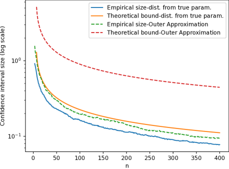
Figure 2: Comparison of the empirical size and the theoretical upper bound on the size in the constant identification case for $m=2,\delta=0.1,n=400,k=1000$.

5 Conclusions

In this paper we have studied the sample complexity of the Sign-Perturbed Sums (SPS) finite-sample, distribution-free system identification method in the case of scalar linear regression problems. We have proved concentration bounds which show that the sizes of the SPS confidence intervals shrink at a geometric rate (around the true parameter). Similar results were proven for the outer approximation of the region. These results are directly relevant, e.g., for multi-armed bandits and various signal processing problems. Furthermore, the results and the applied techniques can serve as stepping stones to study the sample complexity of SPS in more complex multidimensional cases. Future research directions include extending the results to more general identification problems.

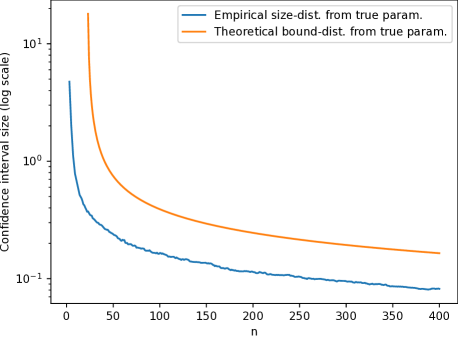
Figure 3: Comparison of the empirical size and the corresponding theoretical bound for scalar linear regression with Gaussian regressors, $m=2,n=400,k=1000$.

References

- Baggio et al. (2022) Baggio, G., Carè, A., Scampicchio, A., and Pillonetto, G. (2022). Bayesian frequentist bounds for machine learning and system identification. Automatica, 146.
- Bercu and Touati (2008) Bercu, B. and Touati, A. (2008). Exponential inequalities for self-normalized martingales with applications. The Annals of Applied Probability, 18(5), 1848–1869.
- Campi and Weyer (2005) Campi, M.C. and Weyer, E. (2005). Guaranteed non-asymptotic confidence regions in system identification. Automatica, 41, 1751–1764.
- Carè et al. (2018) Carè, A., Csáji, B.Cs., Campi, M., and Weyer, E. (2018). Finite-sample system identification: An overview and a new correlation method. IEEE Control Systems Letters, 2(1), 61 – 66.
- Carè et al. (2021) Carè, A., Campi, M., Csáji, B.Cs., and Weyer, E. (2021). Facing undermodelling in Sign-Perturbed-Sums system identification. Systems and Control Letters, 153, 104936.
- Carè (2022) Carè, A. (2022). A simple condition for the boundedness of Sign-Perturbed-Sums (SPS) confidence regions. Automatica, 139, 110150.
- Csáji et al. (2015) Csáji, B.Cs., Campi, M.C., and Weyer, E. (2015). Sign-Perturbed Sums: A new system identification approach for constructing exact non-asymptotic confidence regions in linear regression models. IEEE Transactions on Signal Processing, 63(1), 169–181.
- Csáji and Weyer (2011) Csáji, B.Cs. and Weyer, E. (2011). System identification with binary observations by stochastic approximation and active learning. In Proceedings of the 50th IEEE CDC and ECC, Orlando, Florida, December 12-15.
- Csáji and Weyer (2015) Csáji, B.Cs. and Weyer, E. (2015). Closed-loop applicability of the Sign-Perturbed Sums method. In 54th IEEE Conference on Decision and Control, 1441–1446.
- Csáji and Horváth (2022) Csáji, B.Cs. and Horváth, B. (2022). Nonparametric, nonasymptotic confidence bands with Paley-Wiener kernels for band-limited functions. IEEE Control Systems Letters, 6, 3355–3360.
- Csáji and Kis (2019) Csáji, B.Cs. and Kis, K.B. (2019). Distribution-free uncertainty quantification for kernel methods by gradient perturbations. Machine Learning, 108(8), 1677–1699.
- Kolumbán et al. (2015) Kolumbán, S., Vajk, I., and Schoukens, J. (2015). Perturbed datasets methods for hypothesis testing and structure of corresponding confidence sets. Automatica, 51, 326–331.
- Lattimore and Szepesvári (2020) Lattimore, T. and Szepesvári, C. (2020). Bandit Algorithms. Cambridge University Press.
- Ljung (1999) Ljung, L. (1999). System Identification: Theory for the User. Prentice Hall, Upper Saddle River, 2nd edition.
- Söderström and Stoica (1989) Söderström, T. and Stoica, P. (1989). System Identification. Prentice Hall International, Hertfordshire, UK.
- Tamás and Csáji (2021) Tamás, A. and Csáji, B.Cs. (2021). Exact distribution-free hypothesis tests for the regression function of binary classification via conditional kernel mean embeddings. IEEE Control Systems Letters, 6, 860–865.
- Volpe et al. (2015) Volpe, V., Csáji, B.Cs., Carè, A., Weyer, E., and Campi, M.C. (2015). Sign-Perturbed Sums (SPS) with instrumental variables for the identification of ARX systems. In 54th IEEE Conference on Decision and Control (CDC), Osaka, Japan, 2115–2120.
- Wainwright (2019) Wainwright, M.J. (2019). High-Dimensional Statistics: A Non-Asymptotic Viewpoint. Cambridge Univ. Press.
- Weyer et al. (2017) Weyer, E., Campi, M.C., and Csáji, B.Cs. (2017). Asymptotic properties of SPS confidence regions. Automatica, 81, 287–294.