Muted Features in the JWST NIRISS Transmission Spectrum of Hot-Neptune LTT 9779 b

Abstract

The hot-Neptune desert is one of the most sparsely populated regions of the exoplanet parameter space, and atmosphere observations of its few residents can provide insights into how such planets have managed to survive in such an inhospitable environment. Here, we present transmission observations of LTT 9779 b, the only known hot-Neptune to have retained a significant H/He-dominated atmosphere, taken with JWST NIRISS/SOSS. The 0.6 – 2.85 µm transmission spectrum shows evidence for muted spectral features, rejecting a perfectly flat line at $>$5$\sigma$. We explore water and methane-dominated atmosphere scenarios for LTT 9779 b’s terminator, and retrieval analyses reveal a continuum of potential combinations of metallicity and cloudiness. Through comparisons to previous population synthesis works and our own interior structure modelling, we are able to constrain LTT 9779 b’s atmosphere metallicity to 20–850$\times$ solar. Within this range of metallicity, our retrieval analyses prefer solutions with clouds at mbar pressures, regardless of whether the atmosphere is water- or methane-dominated — though cloud-free atmospheres with metallicities $>$500$\times$ solar cannot be entirely ruled out. By comparing self-consistent atmosphere temperature profiles with cloud condensation curves, we find that silicate clouds can readily condense in the terminator region of LTT 9779 b. Advection of these clouds onto the day-side could explain the high day-side albedo previously inferred for this planet and be part of a feedback loop aiding the survival of LTT 9779 b’s atmosphere in the hot-Neptune desert.

1 Introduction

In the decades since the discovery of the first transiting exoplanet around a Sun-like star (Charbonneau et al., 2000), transit and radial velocity measurements have revealed the parameter space of close-in exoplanets (Borucki et al., 2010; Hartman et al., 2012; Hébrard et al., 2013; Hellier et al., 2014; Delrez et al., 2016; Cloutier et al., 2017; Radica et al., 2022a). Population-level studies of exoplanets have revealed several peculiar demographic features; one of particular interest being the hot-Neptune desert (Szabó & Kiss, 2011; Mazeh et al., 2016, Fig. 1) — a dearth of Neptune-mass planets with orbital periods shorter than $\sim$4 d, which cannot be explained by observational biases. The hot-Neptune desert is predicted to be carved out by photoevaporation driven by high energy radiation from the host star (Owen & Wu, 2013; Owen & Lai, 2018). Jupiter-mass planets are massive enough to retain the bulk of their atmosphere against photoevaporation, whereas smaller planets lose their entire gaseous envelope on short timescales ($<$100 Myr; Owen & Wu, 2013) leaving behind bare rocky cores, with perhaps trace amounts of an atmosphere (e.g., Armstrong et al., 2020). Indeed, studies of atmosphere escape, via e.g., the 1.083 µm metastable He triplet (Seager & Sasselov, 2000; Oklopčić & Hirata, 2018), have demonstrated that many of the planets bordering the hot-Neptune desert are currently experiencing substantial mass loss (Spake et al., 2018; Allart et al., 2018, 2023).

LTT 9779 b (Jenkins et al., 2020) is one of only a handful of known hot-Neptunes. With a mass of 29.32$\pm$0.8 M_⊕, a radius of 4.72$\pm$0.23 R_⊕, and a 0.792 d period, it resides right in the heart of the hot-Neptune desert (Fig. 1, Jenkins et al., 2020). Despite orbiting in this inhospitable region of parameter space, observations with the Spitzer Space Telescope’s Infrared Array Camera (IRAC) provided evidence for a substantial H/He-rich atmosphere, with a metallicity $>$30$\times$ solar (Dragomir et al., 2020; Crossfield et al., 2020). Spitzer/IRAC eclipse observations also revealed a day-side brightness temperature of $>$2300 K at 3.6 µm — equivalent to some of the hottest hot-Jupiters (Hartman et al., 2012; Delrez et al., 2016; Mansfield et al., 2021).

Recently, Hoyer et al. (2023) presented the detection of the optical eclipse of LTT 9779 b with a depth of 115$\pm$24 ppm using the Charaterising Exoplanets Satellite (CHEOPS), indicating an extremely high ($\sim$0.8) day-side geometric albedo. Their 1D self-consistent models suggest that the high optical albedo is caused by silicate clouds on the day-side, which due to the planet’s extreme day-side temperature, can only be possible if the atmospheric metallicity is $\gtrsim$400$\times$ solar (Hoyer et al., 2023). An analysis of follow-up observations with the UVIS mode of the Hubble Space Telescope (HST) is also underway to confirm this high albedo in the near-ultraviolet. However, transmission observations with HST’s Wide Field Camera 3 (WFC3) G102 and G141 grisms presented by Edwards et al. (2023) suggest a cloud-free terminator and a very low (subsolar) atmospheric metallicity. They also find no evidence for atmospheric escape via an analysis of the He 1.083 µm metastable triplet.

Finally, Fernández Fernández et al. (2024) recently published an upper limit on the XUV flux of LTT 9779 using XMM-Newton. They indicate that the X-ray faintness of the G7V host star likely played a major role in the long-term survival of LTT 9779 b’s atmosphere.

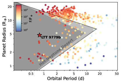
Figure 1: The population of close-in exoplanets visualized in period-radius space. All confirmed planets (from the NASA Exoplanet Archive), with masses and radii measured to better than 15% and 10% respectively, are shown coloured by the amount of flux they receive from their host star relative to the Earth. The hot-Neptune desert, as defined by Mazeh et al. (2016), is marked in grey, and LTT 9779 b is identified with a star.

Here we present a transmission spectrum of LTT 9779 b with the Single Object Slitless Spectroscopy (SOSS) mode (Albert et al., 2023) of JWST’s Near Infrared Imager and Slitless Spectrograph (NIRISS) instrument (Doyon et al., 2023). This is the first paper in a three-part series: Coulombe et al. (submitted) presents a complementary analysis of the full NIRISS/SOSS phase curve of LTT 9779 b, and Radica et al. (in prep) will follow up with an in-depth analysis of the secondary eclipse spectrum. This manuscript is organized as follows: we briefly outline the observations and data reduction in Section 2, and the light curve fitting in Section 3. We then describe our atmosphere modelling in Section 4, follow up with a discussion in Section 5, and concluding remarks in Section 6.

2 Observations and Data Reduction

We observed a full-orbit phase curve of LTT 9779 b with NIRISS/SOSS as part of GTO 1201 (PI: Lafrenière), starting on Jul 7, 2022 at 01:29:06 UTC and lasting 21.9 hours. We operated SOSS in the SUBSTRIP256 readout mode, which provides access to the second diffraction order containing wavelengths shorter than $\sim$0.85 µm (Albert et al., 2023). We thus obtained the full spectral coverage of SOSS, from 0.6 – 2.85 µm. The time series observations (TSO) used ngroup=2 and consisted of 4790 total integrations.

The data reduction and validation are treated more fully in Coulombe et al. (submitted), but for completeness, the pertinent points are summarized below. We reduced the full phase curve using the supreme-SPOON pipeline (Radica et al., 2023; Feinstein et al., 2023; Lim et al., 2023; Fournier-Tondreau et al., 2023), following Stages 1 – 3 as laid out in Radica et al. (2023). We extracted the 1D stellar spectra using a simple box aperture since the effects of the SOSS self-contamination are predicted to be negligible for this target (Darveau-Bernier et al., 2022; Radica et al., 2022b). We used an extraction width of 40 pixels, which we found to minimize the out-of-transit scatter in the extracted spectra.

In order to ensure that our results are robust against the particularities of a given reduction pipeline, we also reduced the full TSO with the NAMELESS pipeline (Feinstein et al., 2023; Coulombe et al., 2023). We performed steps of Stages 1 and 2 as described in Coulombe et al. (2023), putting special emphasis on the correction of cosmic rays and 1/$f$ as we found those two effects to be the main contributors of scatter in the extracted spectra. Cosmic rays were detected and clipped using a running median of the individual pixel counts (see Coulombe et al., submitted for a more in-depth description). As for the 1/$f$ noise, we used the method of Coulombe et al. (2023) and considered only pixels less than 30 pixels away from the trace to compute the 1/$f$, similar to what is done in Feinstein et al. (2023) and Holmberg & Madhusudhan (2023), as we found this method to significantly reduce scatter at longer wavelengths.

3 Light Curve Fitting

In this work, we focus solely on the transit portion of the phase curve observations. We compare two methods of extracting the transmission spectrum from the observations: Method 1 uses the supreme-SPOON reduction, and fits light curves from the portion of the phase curve surrounding the transit. Method 2 uses the NAMELESS reduction and simultaneously fits the entire phase curve.

3.1 Method 1: Transit Fitting

Using the supreme-SPOON reduction, we extract from the phase curve the integrations containing the transit of LTT 9779 b (integrations 2000 – 3000 or BJD 2459767.44667 – 2459767.63738). We opt for a slightly longer ($\sim$3.5:1) baseline in order to better constrain high-frequency variations in the TSO, which we attribute to stellar granulation (Coulombe et al. submitted). In total, our transit observations last 4.57 hours, with 2 hours before and 1.7 hours after the $\sim$47-minute transit.

3.1.1 White Light Curve Fitting

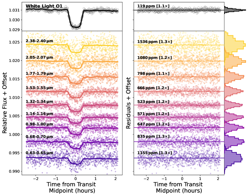
Figure 2: LTT 9779 b transit light curve fits. Left: Order 1 white light curve, and examples of 10 spectrophotometric transit light curves (open points) and their best-fitting transit models (solid lines) from the supreme-SPOON reduction. The wavelength extent of each bin is shown above the best-fitting model. Right: Residuals to each best-fitting model. The scatter in the residuals in ppm is noted above each, as well as, in brackets, its multiple above the predicted photon noise level. Histograms of the residuals are shown to the right.

We construct white light curves for each of the two SOSS orders by summing the flux from all wavelengths in order 1 and wavelengths $<$0.85 µm in order 2. We jointly fit two transit models to the white light curves. Each transit model consists of an astrophysical model and a “systematics” model. The astrophysical model is a standard batman transit model (Kreidberg, 2015). We fix the orbital period to 0.79207022 d, and assume a circular orbit (Crossfield et al., 2020). The planet’s orbital parameters, that is the time of mid-transit, $T_{0}$, the impact parameter, $b$, and the scaled semi-major axis, $a/R_{*}$ are shared between both orders, whereas we individually fit the transit radius, $R_{p}/R_{*}$, as well as the two parameters of the quadratic limb-darkening law, $u_{1}$ and $u_{2}$, to each order.

The “systematics” model takes care of everything that is not the planetary transit. Low-frequency, non-Gaussian noise is clearly visible in the out-of-transit baseline. Coulombe et al. (submitted) conclude that these deviations are likely caused by granulation in the host star’s photosphere (e.g., Kallinger et al., 2014; Grunblatt et al., 2017; Pereira et al., 2019), and correct its effects using a Gaussian Process (GP) with simple harmonic oscillator (SHO) kernel. We follow the same prescription here. Using celerite (Foreman-Mackey, 2017) we fit the two parameters of a SHO GP, $a_{gran}$ and $b_{gran}$ — corresponding to the amplitude and characteristic timescale of the granulation signal (Pereira et al., 2019). The timescale is shared between both orders, however, the GP amplitude is individually fit. Furthermore, for each order we fit for the transit baseline zero-point, as well as a linear trend to account for the planet’s phase variation, and the long-term slope seen in the full phase curve data (Coulombe et al. submitted). Lastly, for each order, we fit an error inflation term added in quadrature to the extracted errors. Our final transit model therefore has 18 parameters: nine for the astrophysical model, and another nine to account for “systematics”. We fit the light curves with juliet’s (Espinoza et al., 2019) implementation of pymultinest (Buchner, 2016), using wide, uninformative priors for all parameters. The white light curve and best fitting model are shown in the top panel of Figure 2, and relevant fitted parameters are summarized in Table 1.

Table 1: Best-fitting white light transit parameters

Parameter	Value
T0 [BJD]	59767.54935$\pm$1.5$\times$10-4
$\rm R_{p}/R_{*,O1}$	0.04749$\pm$0.00261
$\rm R_{p}/R_{*,O2}$	0.04623$\pm$0.00308
$\rm b$	0.91687$\pm$0.00903
$\rm a/R_{*}$	3.80948$\pm$0.13473
$\rm a_{gran,O1}$ [ppm]	68.66$\pm$20.04
$\rm a_{gran,O2}$ [ppm]	95.73$\pm$29.35
$\rm b_{gran}$ [min]	24.97$\pm$8.08

• Notes: Subscripts O1 and O2 refer to values from the order 1 and order 2 white light curves respectively. Parameters without an order subscript were jointly fit to both orders.

3.1.2 Spectrophotometric Light Curve Fitting

We create spectrophotometric light curves by binning the data to a constant resolution of $R$=150. We choose $R$=150 as it results in a sufficient signal-to-noise in the binned light curves to accurately model the aforementioned systematics, though we note that our results remain unchanged if we instead fit at a higher resolution. Furthermore, binning the light curve before fitting results in more accurate transit depth precisions compared to a fitting-then-binning scheme, which inherently assumes that individual bins are uncorrelated, which, particularly for small bins, may not be the case (Holmberg & Madhusudhan, 2023).

We fix the orbital parameters in the spectrophotometric fits to those obtained from the transit fits (Table 1), and the quadratic limb-darkening parameters to model predictions from ExoTiC-LD (Grant & Wakeford, 2022) using the 3D Stagger grid (Magic et al., 2015), as the planet’s high inclination ($\sim$76^o) makes it impossible to accurately back-out the stellar limb-darkening from the transit light curves (Müller et al., 2013). When freely fit, the limb-darkening remains entirely unconstrained across the full prior range and a spurious upward slope towards redder wavelengths is introduced into the transmission spectrum. We also note that our results presented below are unchanged if we instead use other (i.e., four-parameter) limb-darkening law. We scale the best-fitting GP model from the white light curve to account for the granulation signal in each of the spectrophotometric light curves, as we find that the granulation noise only varies in amplitude with wavelength (becoming less prominent towards redder wavelengths) and not its overall structure. We also fit for the transit zero point and a linear trend. Our spectrophotometric light curve model therefore consists of five parameters. Examples of several bins and their best-fitting models are shown in Figure 2.

3.2 Method 2: Phase Curve Fitting

Once again, the phase curve fitting methodology is outlined in further detail in Coulombe et al. (submitted), but we provide a short summary here. Given the extreme equilibrium temperature of LTT 9779 b, it is possible that the “dark planet” assumption inherent in our transit-only fits breaks down and our retrieved transit depths are biased by non-negligible night side flux (Kipping & Tinetti, 2010). However, by fitting the full phase curve, we naturally account for the potential for the planet to have non-zero night side flux (e.g., Martin-Lagarde et al., 2020).

The phase curve fits were performed considering a 12-parameter slice model, with the planetary surface being divided into six longitudinal slices for which we each fit a thermal emission and albedo value, describing the variation of the planetary flux throughout its orbit (e.g., Cowan & Agol, 2011). For the white light fit, instead of using the two SOSS orders as was done with the transit-only analysis above, we constructed a phase curve dominated by reflected-light emission, using wavelengths $<$1 µm, such that we needed only to consider albedo, in addition to a systematics model consisting of a SHO GP and linear slope as described in Section 3.1.1, at the white-light curve stage. This choice was made in order to enable the best-possible correction of the granulation signal, as we found that fitting for the albedo and thermal emission in addition to the SHO GP led to the phase curve model absorbing some of the granulation signal; resulting in nonphysical solutions.

Both thermal emission and reflected light were then accounted for in the fits for each spectrophotometric bin. To extract a transmission spectrum, we fit for the planetary radius and limb-darkening coefficients at each wavelength. The orbital parameters were fixed to the values from Table 1, and the limb-darkening coefficients to the same values considered in the transit-only analysis for easier comparison between the two reductions. Finally, for each bin we considered a linear slope as well as the scaled best-fitting white light curve GP for our spectroscopic systematics model.

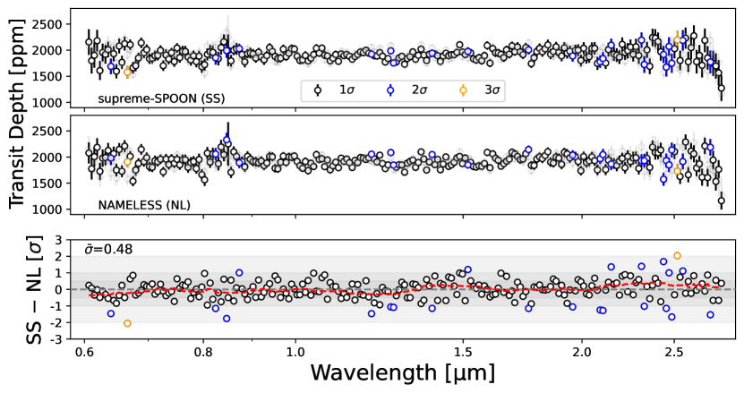
Figure 3: Comparison between supreme-SPOON and NAMELESS transmission spectra. Top: supreme-SPOON transmission spectrum with points colored by their deviation from the NAMELESS spectrum. Black points are consistent between the two spectra at a 1$\sigma$ level, blue points at 2$\sigma$, etc. Sigma levels are calculated using the maximum error bar between the two spectra for each wavelength bin. The NAMELESS spectrum is also shown in faded points. Middle: Same as the top panel, but for the NAMELESS spectrum. Bottom: Differences in each spectral bin divided by the maximum error bar of the two reductions. The red dashed line is a running median showing that there are no low-frequency trends. The average deviation between the two spectra is 0.48$\sigma$.

3.3 Spectrum Consistency

There is good agreement between the supreme-SPOON and NAMELESS transmission spectra, which have not only been reduced with independent pipelines but also fit with different methodologies (Figure 3). The spectra are consistent with each other at a 0.48$\sigma$ level, on average, with no systematic biases. Nevertheless, we recognize that even small deviations, or single outliers between spectra that look consistent by-eye can lead retrievals to divergent inferences (e.g., Welbanks et al., 2023). We thus conduct our analysis on a combination of our two transmission spectra to pseudo-marginalize over any differences in data reduction and light curve fitting techniques (e.g., Bell et al., 2023). We thus create a combined transmission spectrum by taking the average of the transit depths in each wavelength bin. We then assign the transit depth error as the maximum of the errors from each spectrum in the case that the points are 1$\sigma$ consistent, or calculate a new error bar by inflating the maximum error until 1$\sigma$ consistency is achieved. In the remainder of this study, we use the combined transmission spectrum, though we note that our results are consistent if we focus on either reduction alone.

4 Atmosphere Modelling

To explore the plausible range of atmospheric scenarios that are consistent with the data, we used the open-source atmospheric retrieval tool CHIMERA (Line et al., 2013; Taylor et al., 2023). We start with a free chemistry retrieval considering the following species which are commonly expected in the atmospheres of transiting planets: H₂O (Polyansky et al., 2018; Freedman et al., 2014), CH₄ (Rothman et al., 2010), CO (Rothman et al., 2010), CO₂ (Freedman et al., 2014), Na (Kramida et al., 2018; Allard et al., 2019) and K (Kramida et al., 2018; Allard et al., 2016), and limit the vertically-constant log abundances of each species between [-12, -1], except for H₂O and CH₄ for which we use [-12, 0] in order to probe extremely high metallicity scenarios which cannot be ruled out for Neptune-mass planets (e.g., Fortney et al., 2013; Moses et al., 2013; Morley et al., 2017). For H/He-dominated atmospheres, we include H₂-H₂ and H₂-He collision-induced absorption (Richard et al., 2012). The isothermal atmosphere temperature can vary between 700–2000 K, based on the range of temperature profiles around the terminator region retrieved by Coulombe et al. (submitted). We also include a grey cloud deck, constrained to pressures between 1 and 10^-6 bar.

We do not consider the transit light source effect (TLSE; Rackham et al., 2018; Lim et al., 2023; Fournier-Tondreau et al., 2023) in our retrievals as LTT 9779 is known to be slowly rotating and thus inactive (Jenkins et al., 2020). Moreover, Edwards et al. (2023) included the TLSE in their HST retrievals but found that it was disfavoured over models without the TLSE, and resulted in unreasonably high spot and faculae filling factors.

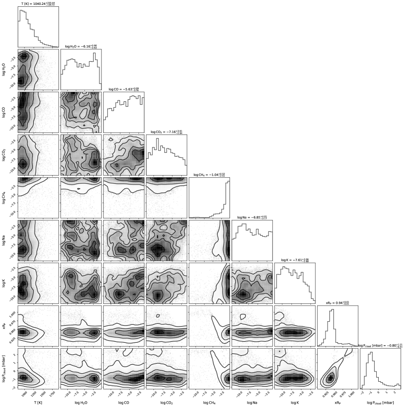
Figure 6: Posterior distributions for the full free chemistry retrieval described in Section 4. There are weak preferences for the presence of H₂O, CH₄, and clouds at sub-mbar pressures. In many cases, the “best-fit” values reported above the marginal distributions are simply the mean of the prior range.

Unsurprisingly, given the muted nature of the spectrum, there are no strong constraints on the atmosphere composition. The retrieval finds evidence for some features due to a combination of H₂O and CH₄, as well as a preference for clouds at $\sim$mbar pressure levels; though constraints on each of these parameters are weak (e.g., Figure 6). The abundances of all other species considered in the retrieval remain unconstrained by the data.

Within the SOSS waveband, transmission observations are primarily sensitive to absorption due to H₂O absorption bands at 1.2, 1.4, 1.8 µm, etc. (Feinstein et al., 2023; Radica et al., 2023; Taylor et al., 2023). Depending on the thermochemical regime of the atmosphere (T$\lesssim$850 K or C/O$>$1), absorption bands of CH₄ could potentially be visible at 1.4, 1.7, 2.3 µm (Moses et al., 2011; Visscher & Moses, 2011; Madhusudhan, 2012). Other major C-bearing molecular species (e.g., CO, CO₂) have negligible opacity in the SOSS waveband and we cannot reasonably expect to constrain them with SOSS observations alone (Taylor et al., 2023).

Based on the above considerations, we conduct a series of nested retrievals to attempt to ascertain whether H₂O or CH₄ is the preferred absorber in LTT 9779 b’s terminator region. We conduct three additional free retrievals; one removing H₂O, another removing CH₄, and a final one removing both molecules. The prior ranges for all included parameters remain the same as stated above. Comparing the model likelihoods from each case, we are unable to determine whether the spectrum is best fit with H₂O ($\rm\log Z=-129.8$), CH₄ ($\rm\log Z=-130.2$), or a combination of both ($\rm\log Z=-129.6$) as the differences between the model evidences in each of the three cases are far from being statistically significant (Benneke & Seager, 2013). However, we find a $>$5$\sigma$ preference for the inclusion of H₂O and/or CH₄ over an atmosphere devoid of either ($\rm\log Z_{flat}=-163.4$).

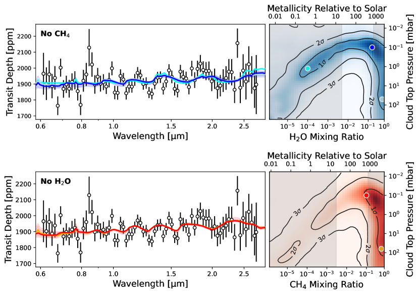
Figure 4: Water and methane dominated atmosphere models for LTT 9779 b.Top Left: Combined transmission spectrum of LTT 9779 b. Overplotted in dark blue is the best-fitting model from our atmosphere retrievals as well as the 1 and 2$\sigma$ credible envelopes. Degeneracy between cloud pressure and metallicity (e.g., Benneke & Seager, 2013; Benneke et al., 2019) allows for solutions with a sub-solar metallicity and deeper clouds (light-blue), as well as with extremely-high ($>$1000$\times$ solar) metallicity and clouds below the observable photosphere (blue-grey). Both data and models are binned to a constant resolution of $R=50$ for visual clarity. Note that the blue-grey model is virtually indistinguishable from the dark blue. Top Right: Two-dimensional correlation between the atmosphere metallicity and cloud top pressure in our retrieved posterior distribution. The coloured points mark the parameter space “locations” of the correspondingly coloured atmosphere model. Grey shading denotes regions of parameter space that can be ruled out by population synthesis and interior modelling work (see Section 5). Bottom: Same as the top, but for the “No H₂O”, CH₄-dominated case. Note that like the dark blue and blue-grey models above, the orange and red models are virtually indistinguishable.

As shown by Coulombe et al. (submitted), LTT 9779 b’s atmosphere undergoes enormous changes in temperature across the terminator region; from $\sim$600 – $\sim$1800 K moving from night to dayside. It is, therefore, possible that light from the host star passing through the planet’s terminator region encounters chemical regimes that are highly nonuniform as a function of longitude; with CH₄ dominating near the colder nightside, and H₂O becoming more prominent closer to the dayside. Our transmission spectrum is then effectively an average over these different regimes. We, therefore, move to consider two end-member scenarios: an atmosphere where the dominant absorbers (in the NIRISS waveband) are H₂O and clouds, and another with CH₄ and clouds. The true state of LTT 9779 b’s terminator likely lies somewhere in between. Using the retrievals described in the previous paragraph, the H₂O/CH₄ vs cloud-pressure posterior distributions for each case as well as some representative atmosphere models are shown in Figure 4.

Finally, since Edwards et al. (2023) find evidence for FeH in their HST/WFC3 spectrum, we perform another free chemistry retrieval, identical to the initial free chemistry retrieval, except also including FeH opacity (Wende et al., 2010). The abundance of FeH remains unconstrained by the data, and we are therefore not able to confirm the results of Edwards et al. (2023). The inference of FeH from HST likely stems from the slope seen in the transmission spectrum, which is not present in our NIRISS observations. We also test for the presence of optical absorbers such as TiO and VO, but as in the case of FeH, we find no evidence for either in the transmission spectrum.

4.1 Interior Structure Modelling

To ensure that our inferred atmosphere compositions are consistent with the measured bulk density of the planet, we run interior structure models in a retrieval framework following Thorngren & Fortney (2019). The models at any given time-step are solutions of the equations of hydrostatic equilibrium, mass conservation, and the material equations of state. We use Chabrier et al. (2019) for the H/He and Thompson (1990) for the metals, which we represent as a 50-50 mixture of rock and ice. Because we are seeking an upper limit on the atmospheric metallicity, we model the conservative case (for that purpose) of a fully-mixed planet. The models are evolved forward in time from a hot initial state using the atmosphere models of (Fortney et al., 2007). As LTT 9799 b is a hot-Neptune, we include the anomalous hot Jupiter heating effect, parameterized in (Thorngren & Fortney, 2018). These models are then used in a Bayesian retrieval framework to find planet bulk metallicities consistent with the planet’s mass, radius, and age (all with uncertainties). We find that LTT 9799 b is indeed a quite metal-rich planet, with $Z_{p}=90\pm 2\%$. Taking the 2-$\sigma$ upper limit of our metal distribution and converting to a number ratio, we obtain a maximum atmosphere metallicity of $\sim$850$\times$ solar.

Additionally, Fortney et al. (2013) conducted a population synthesis study to attempt to predict, a-priori, the possible atmosphere metallicities of transiting planets, including those of Neptune-like masses. They show that metallicities in excess of 1000$\times$ solar are to be expected, however, they do not find a single Neptune-mass planet with a metallicity $<$20$\times$ solar. This fits in with trends observed in both the solar system and transiting exoplanets (e.g., Welbanks et al., 2019). We can therefore set a rough lower limit for the possible metallicity of LTT 9779 b’s atmosphere at $\sim$20$\times$ solar. This constraint, and that from interior structure models are shown as grey shaded regions in Figure 4, and substantially restrict the possible parameter space of atmosphere compositions.

4.2 Searching for Tracers of Atmosphere Escape

Finally, we inspected the pixel-level (that is; one light curve per detector pixel column) transit depths near 1.083 µm for evidence of excess absorption due to the metastable He triplet (Oklopčić & Hirata, 2018; Spake et al., 2018). Due to its extreme level of irradiation, LTT 9779 b receives $>$2500$\times$ more flux from its host star than the Earth, it might be expected to be in the process of losing its atmosphere through photoevaporation (Owen & Wu, 2013; Owen & Lai, 2018). However, like Edwards et al. (2023), we find no clear evidence for He absorption in our spectrum.

Nevertheless, we attempt to assess the strength of any potential He signal in the data, which may not be obvious by-eye, by fitting a Gaussian to the pixel-level transmission spectrum. The Gaussian He model has a fixed full-width-half-maximum of $\sim$0.75 Å (comparable to values reported by Allart et al. (2018) and Allart et al. (2023)), and centered at 1.0833 Å  but with a free amplitude convolved to the resolution of NIRISS/SOSS (R$\sim$700). The fitted amplitude seen at the full resolution of SOSS is 0.15$\pm$0.61 $\%$ (as a comparison the helium signature measured for HD 189733b is $\sim$0.7$\%$; e.g., Salz et al., 2018; Guilluy et al., 2020; Allart et al., 2023).

LTT 9779, though, is a G7V star and it is thought that the UV spectra of K-type stars are more conducive to populating the metastable He triplet state (Oklopčić, 2019). The lack of a metastable He detection therefore may not mean that LTT 9779 b is not undergoing significant mass loss, but that this mass loss cannot be probed optimally via the 1.083 µm metastable He triplet. Other mass-loss tracers like Ly-$\alpha$ (the system is only at a distance of 80 pc and interstellar medium absorption might not be completely optically thick), or lines of ionized metal (Linssen & Oklopčić, 2023) may prove to be more fruitful tracers of atmospheric escape around sun-like stars. SOSS is also potentially able to probe atmosphere loss via H$\alpha$ (Vidal-Madjar et al., 2003; Lim et al., 2023; Howard et al., 2023), though we also find no evidence for excess H$\alpha$ absorption in our data. Thus, as proposed by Fernández Fernández et al. (2024), due to the weak high-energy emission of the host star LTT 9779 b may simply not be undergoing sufficiently significant photoevaporative mass loss for any of the aforementioned tracers to be observable.

5 Discussion

Our transmission spectrum of the unique hot-Neptune LTT 9779 b is relatively featureless and our retrievals thus prefer solutions with negligible feature amplitudes (Figure 4). The retrievals are able to create a flat transmission spectrum with three broad families of solutions: one with very sub-solar ($<$0.1$\times$ solar) metallicity, one with super-solar metallicity and low-pressure (P$\rm{}_{cloud}\lesssim 1$ mbar) clouds, and a final family with extremely high ($>$500$\times$ solar) metallicity (Figure 4). This is a manifestation of the well-known cloud-metallicity degeneracy (e.g., Benneke & Seager, 2013; Knutson et al., 2014; Benneke et al., 2019): a low column density of H₂O or CH₄ vapour is the primary cause of the lack of features in the low metallicity case, whereas the feature amplitudes in the second family of models are dampened by clouds. In the final model family, the atmosphere metallicity is sufficiently elevated to reduce the atmosphere scale height and attenuate the amplitude of molecular features without needing to invoke clouds.

Due to the flatness of LTT 9779 b’s transmission spectrum, we are not able to make any strong claims about the atmosphere composition from the transit observations alone. Previous studies of canonical Neptune-mass planets such as GJ 436 b have demonstrated that exotic atmosphere compositions, with metallicities in excess of 1000$\times$ solar, are indeed possible (Fortney et al., 2013; Moses et al., 2013; Morley et al., 2017). However, we can begin to limit the parameter space of possible atmosphere compositions through arguments of self-consistency. In particular, our interior structure upper limit rules out high-metallicity/cloud-free atmospheres at $\sim$2$\sigma$, and population synthesis constraints remove the low-metallicity scenarios; irrespective of whether H₂O or CH₄ is assumed to be the dominant absorber. The most likely family of solutions thus becomes that with elevated metallicity between $\sim$20 and 850$\times$ solar, and clouds at $\sim$mbar pressure levels — though atmospheres with metallicities $>$500$\times$ solar and cloud-free photospheres cannot be entirely ruled out.

An atmosphere with an elevated metallicity and clouds is consistent with findings from previous studies of this planet. In particular Hoyer et al. (2023) and Coulombe et al. (submitted) both find evidence for a high dayside albedo ($A_{g}$ = 0.6 – 0.8). As shown in both of those works, the presence of reflective, high-altitude clouds can account for this elevated albedo. The cloud-free low or high metallicity scenarios allowed by our data would thus not be consistent with previous findings. In theory, exotic cloud species could emerge at the extreme high-metallicity end of our probed parameter space. Moses et al. (2013), in particular, explore the condensation of graphite in $>$1000$\times$ solar, carbon-rich atmospheres of Neptune-mass planets, and conclude that it is unlikely to build up in the photosphere in sufficient concentrations to affect transmission spectra.

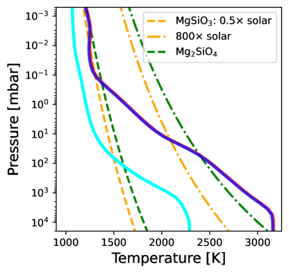
Figure 5: Exploration of cloud formation in LTT 9779 b’s terminator region via a comparison of terminator PT profiles and condensation curves of prominent silicate clouds species. PT profiles were calculated self-consistently using the SCARLET framework (Benneke, 2015), for three of the cases shown in Figure 4: sub-solar metallicity H₂O-dominated (light blue), super-solar metallicity H₂O-dominated (dark blue), and super-solar metallicity CH₄-dominated (red). Condensation curves are from Visscher et al. (2010) and calculated at two metallicities: 0.5$\times$ solar (dashed), 800$\times$ solar (dot-dashed), reflecting the sub- and super-solar metallicity models shown. The terminator temperature of LTT 9779 b is sufficiently cool to allow for silicate clouds to readily condense at millibar pressures, even for sub-solar atmospheric metallicities. Note that the red and dark blue PT profiles are entirely overlapping.

Based on the above considerations, we explore the thermochemistry of possible cloud condensation with our retrieved terminator conditions. Using the SCARLET framework (Benneke, 2015), we generate self-consistent atmosphere pressure-temperature (PT) profiles for metallicities of $\sim$0.5$\times$ and $\sim$800$\times$ solar, corresponding to the light blue and dark blue/red models in Figure 4, respectively. The models were computed considering a bond albedo of $A_{B}$ = 0.66, heat redistribution of $f$ = 0.5 (uniform dayside), and no opacity from optical absorbers such as TiO and VO (which would lead to a temperature inversion) as informed from the thermal emission retrievals shown in Coulombe et al. (submitted). We show these PT profiles, as well as condensation curves for enstatite (MgSiO₃) and forsterite (Mg₂SiO₄) from Visscher et al. (2010) in Figure 5, demonstrating that silicate clouds can readily condense at mbar levels in LTT 9779 b’s terminator region, even at solar atmospheric metallicities. Advection of these clouds onto the day-side could then cause the high albedo reported by Hoyer et al. (2023).

Though the low XUV output of the host star likely renders any photoevaporative mass loss processes very inefficient (e.g., Fernández Fernández et al., 2024), a core-powered mass loss mechanism (that is, mass loss driven by the host star’s bolometric luminosity as opposed to just its high-energy output; e.g., Ginzburg et al., 2018; Gupta & Schlichting, 2021) may still be impactful. We posit that a cloudy nature for LTT 9779 b’s atmosphere may be part of a positive feedback loop that suppresses the effectiveness of atmospheric loss and contributes to its survival in the desert. For instance, following Seager (2010), the equilibrium temperature of a planet can be calculated;

$$T_{\mathrm{eq}}=T_{\mathrm{eff,*}}\bigg{(}\frac{R_{*}}{a}\bigg{)}^{1/2}[f(1-A_{\mathrm{B}})]^{1/4}$$ (1)

where $T_{\mathrm{eff,*}}$ is the host star effective temperature, $A_{\mathrm{B}}$ the planet’s bond albedo, and $f$ a factor describing heat recirculation. Assuming partial heat recirculation (Hoyer et al., 2023) and the scaled semi-major axis and host star temperature from Jenkins et al. (2020), increasing the bond albedo from 0 to $\sim$0.7 (consistent with Hoyer et al. (2023) and Coulombe et al. (submitted)), results in a decrease in $T_{\mathrm{eq}}$ from $\sim$2300 K to $\sim$1600 K. Again, following Seager (2010), the thermal escape parameter, $\lambda_{c}$, is;

$$\lambda_{c}=\frac{m_{\mathrm{H}}g_{\mathrm{e}}r_{\mathrm{e}}}{k_{\mathrm{B}}T_{\mathrm{e}}}$$ (2)

where $g_{\mathrm{e}}$, $r_{\mathrm{e}}$, and $T_{\mathrm{e}}$ are the gravity, radius, and temperature respectively of the exobase, and $m_{\mathrm{H}}$ the mass of hydrogen. Smaller escape parameters correspond to larger escape fluxes via $F_{esc}\propto(1+\lambda_{c})e^{-\lambda_{c}}$. Assuming that the exobase temperature is proportional to the equilibrium temperature results in an increase in the escape parameter by a factor of $\sim$1.5 for the $A_{\mathrm{B}}=0.7$ compared to the $A_{\mathrm{B}}=0$ case. Though this is not enough to completely halt any escape processes, or change the escape regime from hydrodynamical to hydrostatic (e.g., Pierrehumbert, 2010), it will, nevertheless, decrease the rate at which the atmosphere is escaping. Supposing LTT 9779 b initially formed as a cloud-free hot-Saturn (e.g., Jenkins et al., 2020; Fernández Fernández et al., 2024), the preferential loss of light elements (i.e., hydrogen) over time could result in an increase in atmosphere metallicity, or decrease in gravity; both of which favour cloud formation (e.g., Stevenson, 2016; Hoyer et al., 2023). Clouds then cause a decrease in the efficiency of atmosphere loss, prolonging the lifetime of the atmosphere.

6 Conclusions

In this work, we have presented the first JWST transmission spectrum of LTT 9779 b; the only known hot-Neptune to have retained a substantial atmosphere. In light of population synthesis and interior modelling considerations, cloudy, high-metallicity solutions are the most likely explanations for our transmission spectrum, regardless of whether we consider a H₂O or CH₄-dominated atmosphere — though our transit data alone also allows for sub-solar and $\sim$1000$\times$ solar metallicity solutions with cloud-free photospheres. Along with Coulombe et al. (submitted), this work lays the groundwork for an understanding of the intriguing hot-Neptune LTT 9779 b. Coupled with the spectrum presented here, future observations of this planet with JWST NIRSpec should have the necessary precision to differentiate between H₂O and CH₄-dominated terminator conditions, and better refine the atmosphere metallicity.

References

- Albert et al. (2023) Albert, L., Lafrenière, D., René, D., et al. 2023, PASP, 135, 075001, doi: 10.1088/1538-3873/acd7a3
- Allard et al. (2016) Allard, N. F., Spiegelman, F., & Kielkopf, J. F. 2016, A&A, 589, A21, doi: 10.1051/0004-6361/201628270
- Allard et al. (2019) Allard, N. F., Spiegelman, F., Leininger, T., & Molliere, P. 2019, A&A, 628, A120, doi: 10.1051/0004-6361/201935593
- Allart et al. (2018) Allart, R., Bourrier, V., Lovis, C., et al. 2018, Science, 362, 1384, doi: 10.1126/science.aat5879
- Allart et al. (2023) Allart, R., Lemée-Joliecoeur, P. B., Jaziri, A. Y., et al. 2023, A&A, 677, A164, doi: 10.1051/0004-6361/202245832
- Armstrong et al. (2020) Armstrong, D. J., Lopez, T. A., Adibekyan, V., et al. 2020, Nature, 583, 39, doi: 10.1038/s41586-020-2421-7
- Astropy Collaboration et al. (2013) Astropy Collaboration, Robitaille, T. P., Tollerud, E. J., et al. 2013, A&A, 558, A33, doi: 10.1051/0004-6361/201322068
- Astropy Collaboration et al. (2018) Astropy Collaboration, Price-Whelan, A. M., Sipőcz, B. M., et al. 2018, AJ, 156, 123, doi: 10.3847/1538-3881/aabc4f
- Bell et al. (2023) Bell, T. J., Welbanks, L., Schlawin, E., et al. 2023, Nature, 623, 709, doi: 10.1038/s41586-023-06687-0
- Benneke (2015) Benneke, B. 2015, Strict Upper Limits on the Carbon-to-Oxygen Ratios of Eight Hot Jupiters from Self-Consistent Atmospheric Retrieval, arXiv. http://arxiv.org/abs/1504.07655
- Benneke & Seager (2013) Benneke, B., & Seager, S. 2013, ApJ, 778, 153, doi: 10.1088/0004-637X/778/2/153
- Benneke et al. (2019) Benneke, B., Wong, I., Piaulet, C., et al. 2019, ApJ, 887, L14, doi: 10.3847/2041-8213/ab59dc
- Borucki et al. (2010) Borucki, W. J., Koch, D., Basri, G., et al. 2010, Science, 327, 977, doi: 10.1126/science.1185402
- Buchner (2016) Buchner, J. 2016, Stat Comput, 26, 383, doi: 10.1007/s11222-014-9512-y
- Bushouse et al. (2022) Bushouse, H., Eisenhamer, J., Dencheva, N., et al. 2022, JWST Calibration Pipeline, 1.7.0, Zenodo, doi: 10.5281/zenodo.7038885
- Chabrier et al. (2019) Chabrier, G., Mazevet, S., & Soubiran, F. 2019, ApJ, 872, 51, doi: 10.3847/1538-4357/aaf99f
- Charbonneau et al. (2000) Charbonneau, D., Brown, T. M., Latham, D. W., & Mayor, M. 2000, The Astrophysical Journal, 529, L45, doi: 10.1086/312457
- Cloutier et al. (2017) Cloutier, R., Astudillo-Defru, N., Doyon, R., et al. 2017, A&A, 608, A35, doi: 10.1051/0004-6361/201731558
- Coulombe et al. (2023) Coulombe, L.-P., Benneke, B., Challener, R., et al. 2023, Nature, 620, 292, doi: 10.1038/s41586-023-06230-1
- Cowan & Agol (2011) Cowan, N. B., & Agol, E. 2011, ApJ, 729, 54, doi: 10.1088/0004-637X/729/1/54
- Crossfield et al. (2020) Crossfield, I. J. M., Dragomir, D., Cowan, N. B., et al. 2020, ApJ, 903, L7, doi: 10.3847/2041-8213/abbc71
- Darveau-Bernier et al. (2022) Darveau-Bernier, A., Albert, L., Talens, G. J., et al. 2022, PASP, 134, 094502, doi: 10.1088/1538-3873/ac8a77
- Delrez et al. (2016) Delrez, L., Santerne, A., Almenara, J.-M., et al. 2016, Mon. Not. R. Astron. Soc., 458, 4025, doi: 10.1093/mnras/stw522
- Doyon et al. (2023) Doyon, R., Willott, C. J., Hutchings, J. B., et al. 2023, PASP, 135, 098001, doi: 10.1088/1538-3873/acd41b
- Dragomir et al. (2020) Dragomir, D., Crossfield, I. J. M., Benneke, B., et al. 2020, ApJ, 903, L6, doi: 10.3847/2041-8213/abbc70
- Edwards et al. (2023) Edwards, B., Changeat, Q., Tsiaras, A., et al. 2023, AJ, 166, 158, doi: 10.3847/1538-3881/acea77
- Espinoza et al. (2019) Espinoza, N., Kossakowski, D., & Brahm, R. 2019, Monthly Notices of the Royal Astronomical Society, 490, 2262, doi: 10.1093/mnras/stz2688
- Feinstein et al. (2023) Feinstein, A. D., Radica, M., Welbanks, L., et al. 2023, Nature, doi: 10.1038/s41586-022-05674-1
- Fernández Fernández et al. (2024) Fernández Fernández, J., Wheatley, P. J., King, G. W., & Jenkins, J. S. 2024, MNRAS, 527, 911, doi: 10.1093/mnras/stad3263
- Foreman-Mackey (2017) Foreman-Mackey, D. 2017, The Astronomical Journal
- Fortney et al. (2007) Fortney, J. J., Marley, M. S., & Barnes, J. W. 2007, ApJ, 659, 1661, doi: 10.1086/512120
- Fortney et al. (2013) Fortney, J. J., Mordasini, C., Nettelmann, N., et al. 2013, ApJ, 775, 80, doi: 10.1088/0004-637X/775/1/80
- Fournier-Tondreau et al. (2023) Fournier-Tondreau, M., MacDonald, R. J., Radica, M., et al. 2023, Near-Infrared Transmission Spectroscopy of HAT-P-18$\,$b with NIRISS: Disentangling Planetary and Stellar Features in the Era of JWST, arXiv. http://arxiv.org/abs/2310.14950
- Freedman et al. (2014) Freedman, R. S., Lustig-Yaeger, J., Fortney, J. J., et al. 2014, ApJS, 214, 25, doi: 10.1088/0067-0049/214/2/25
- Ginzburg et al. (2018) Ginzburg, S., Schlichting, H. E., & Sari, R. 2018, MNRAS, 476, 759, doi: 10.1093/mnras/sty290
- Grant & Wakeford (2022) Grant, D., & Wakeford, H. R. 2022, Exo-TiC/ExoTiC-LD: ExoTiC-LD v3.0.0, v3.0.0, Zenodo, doi: 10.5281/zenodo.7437681
- Grunblatt et al. (2017) Grunblatt, S. K., Huber, D., Gaidos, E., et al. 2017, AJ, 154, 254, doi: 10.3847/1538-3881/aa932d
- Guilluy et al. (2020) Guilluy, G., Andretta, V., Borsa, F., et al. 2020, A&A, 639, A49, doi: 10.1051/0004-6361/202037644
- Gupta & Schlichting (2021) Gupta, A., & Schlichting, H. E. 2021, MNRAS, 504, 4634, doi: 10.1093/mnras/stab1128
- Harris et al. (2020) Harris, C. R., Millman, K. J., van der Walt, S. J., et al. 2020, Nature, 585, 357, doi: 10.1038/s41586-020-2649-2
- Hartman et al. (2012) Hartman, J. D., Bakos, G. A., Béky, B., et al. 2012, The Astronomical Journal, 144, 139, doi: 10.1088/0004-6256/144/5/139
- Hellier et al. (2014) Hellier, C., Anderson, D. R., Cameron, A. C., et al. 2014, Monthly Notices of the Royal Astronomical Society, 440, 1982, doi: 10.1093/mnras/stu410
- Holmberg & Madhusudhan (2023) Holmberg, M., & Madhusudhan, N. 2023, Monthly Notices of the Royal Astronomical Society, 524, 377, doi: 10.1093/mnras/stad1580
- Holmberg & Madhusudhan (2023) Holmberg, M., & Madhusudhan, N. 2023, MNRAS, 524, 377, doi: 10.1093/mnras/stad1580
- Howard et al. (2023) Howard, W. S., Kowalski, A. F., Flagg, L., et al. 2023, ApJ, 959, 64, doi: 10.3847/1538-4357/acfe75
- Hoyer et al. (2023) Hoyer, S., Jenkins, J. S., Parmentier, V., et al. 2023, A&A, 675, A81, doi: 10.1051/0004-6361/202346117
- Hunter (2007) Hunter, J. D. 2007, Computing in Science & Engineering, 9, 90, doi: 10.1109/MCSE.2007.55
- Hébrard et al. (2013) Hébrard, G., Collier Cameron, A., Brown, D. J. A., et al. 2013, A&A, 549, A134, doi: 10.1051/0004-6361/201220363
- Jenkins et al. (2020) Jenkins, J. S., Díaz, M. R., Kurtovic, N. T., et al. 2020, Nat Astron, 4, 1148, doi: 10.1038/s41550-020-1142-z
- Kallinger et al. (2014) Kallinger, T., De Ridder, J., Hekker, S., et al. 2014, A&A, 570, A41, doi: 10.1051/0004-6361/201424313
- Kipping & Tinetti (2010) Kipping, D. M., & Tinetti, G. 2010, MNRAS, 407, 2589, doi: 10.1111/j.1365-2966.2010.17094.x
- Knutson et al. (2014) Knutson, H. A., Benneke, B., Deming, D., & Homeier, D. 2014, Nature, 505, 66, doi: 10.1038/nature12887
- Kramida et al. (2018) Kramida, A., Yu. Ralchenko, Reader, J., & and NIST ASD Team. 2018, NIST Atomic Spectra Database (ver. 5.6.1), [Online]. Available: https://physics.nist.gov/asd [2019, February 6]. National Institute of Standards and Technology, Gaithersburg, MD.
- Kreidberg (2015) Kreidberg, L. 2015, Publications of the Astronomical Society of the Pacific, 127, 1161, doi: 10.1086/683602
- Lim et al. (2023) Lim, O., Benneke, B., Doyon, R., et al. 2023, ApJL, 955, L22, doi: 10.3847/2041-8213/acf7c4
- Line et al. (2013) Line, M. R., Wolf, A. S., Zhang, X., et al. 2013, ApJ, 775, 137, doi: 10.1088/0004-637X/775/2/137
- Linssen & Oklopčić (2023) Linssen, D. C., & Oklopčić, A. 2023, A&A, 675, A193, doi: 10.1051/0004-6361/202346583
- Madhusudhan (2012) Madhusudhan, N. 2012, ApJ, 758, 36, doi: 10.1088/0004-637X/758/1/36
- Magic et al. (2015) Magic, Z., Chiavassa, A., Collet, R., & Asplund, M. 2015, A&A, 573, A90, doi: 10.1051/0004-6361/201423804
- Mansfield et al. (2021) Mansfield, M., Line, M. R., Bean, J. L., et al. 2021, Nat Astron, 5, 1224, doi: 10.1038/s41550-021-01455-4
- Martin-Lagarde et al. (2020) Martin-Lagarde, M., Morello, G., Lagage, P.-O., Gastaud, R., & Cossou, C. 2020, AJ, 160, 197, doi: 10.3847/1538-3881/abac09
- Mazeh et al. (2016) Mazeh, T., Holczer, T., & Faigler, S. 2016, A&A, 589, A75, doi: 10.1051/0004-6361/201528065
- Morley et al. (2017) Morley, C. V., Knutson, H., Line, M., et al. 2017, AJ, 153, 86, doi: 10.3847/1538-3881/153/2/86
- Moses et al. (2011) Moses, J. I., Visscher, C., Fortney, J. J., et al. 2011, ApJ, 737, 15, doi: 10.1088/0004-637X/737/1/15
- Moses et al. (2013) Moses, J. I., Line, M. R., Visscher, C., et al. 2013, ApJ, 777, 34, doi: 10.1088/0004-637X/777/1/34
- Müller et al. (2013) Müller, H. M., Huber, K. F., Czesla, S., Wolter, U., & Schmitt, J. H. M. M. 2013, A&A, 560, A112, doi: 10.1051/0004-6361/201322079
- Oklopčić (2019) Oklopčić, A. 2019, ApJ, 881, 133, doi: 10.3847/1538-4357/ab2f7f
- Oklopčić & Hirata (2018) Oklopčić, A., & Hirata, C. M. 2018, ApJ, 855, L11, doi: 10.3847/2041-8213/aaada9
- Owen & Lai (2018) Owen, J. E., & Lai, D. 2018, Monthly Notices of the Royal Astronomical Society, 479, 5012, doi: 10.1093/mnras/sty1760
- Owen & Wu (2013) Owen, J. E., & Wu, Y. 2013, ApJ, 775, 105, doi: 10.1088/0004-637X/775/2/105
- Pereira et al. (2019) Pereira, F., Campante, T. L., Cunha, M. S., et al. 2019, Monthly Notices of the Royal Astronomical Society, 489, 5764, doi: 10.1093/mnras/stz2405
- Pérez & Granger (2007) Pérez, F., & Granger, B. E. 2007, Computing in Science and Engineering, 9, 21, doi: 10.1109/MCSE.2007.53
- Pierrehumbert (2010) Pierrehumbert, R. T. 2010, Principles of Planetary Climate (Cambridge University Press)
- Polyansky et al. (2018) Polyansky, O. L., Kyuberis, A. A., Zobov, N. F., et al. 2018, MNRAS, 480, 2597, doi: 10.1093/mnras/sty1877
- Rackham et al. (2018) Rackham, B. V., Apai, D., & Giampapa, M. S. 2018, ApJ, 853, 122, doi: 10.3847/1538-4357/aaa08c
- Radica et al. (2022a) Radica, M., Artigau, E., Lafreniére, D., et al. 2022a, Monthly Notices of the Royal Astronomical Society, 517, 5050, doi: 10.1093/mnras/stac3024
- Radica et al. (2022b) Radica, M., Albert, L., Taylor, J., et al. 2022b, PASP, 134, 104502, doi: 10.1088/1538-3873/ac9430
- Radica et al. (2023) Radica, M., Welbanks, L., Espinoza, N., et al. 2023, Monthly Notices of the Royal Astronomical Society, 524, 835, doi: 10.1093/mnras/stad1762
- Richard et al. (2012) Richard, C., Gordon, I. E., Rothman, L. S., et al. 2012, J. Quant. Spec. Radiat. Transf., 113, 1276, doi: 10.1016/j.jqsrt.2011.11.004
- Rothman et al. (2010) Rothman, L. S., Gordon, I. E., Barber, R. J., et al. 2010, J. Quant. Spec. Radiat. Transf., 111, 2139, doi: 10.1016/j.jqsrt.2010.05.001
- Salz et al. (2018) Salz, M., Czesla, S., Schneider, P. C., et al. 2018, A&A, 620, A97, doi: 10.1051/0004-6361/201833694
- Seager (2010) Seager, S. 2010, Exoplanet Atmospheres: Physical Processes (Princeton University Press)
- Seager & Sasselov (2000) Seager, S., & Sasselov, D. D. 2000, ApJ, 537, 916, doi: 10.1086/309088
- Spake et al. (2018) Spake, J. J., Sing, D. K., Evans, T. M., et al. 2018, Nature, 557, 68, doi: 10.1038/s41586-018-0067-5
- Stevenson (2016) Stevenson, K. B. 2016, ApJ, 817, L16, doi: 10.3847/2041-8205/817/2/L16
- Szabó & Kiss (2011) Szabó, G. M., & Kiss, L. L. 2011, ApJ, 727, L44, doi: 10.1088/2041-8205/727/2/L44
- Taylor et al. (2023) Taylor, J., Radica, M., Welbanks, L., et al. 2023, Monthly Notices of the Royal Astronomical Society, 524, 817, doi: 10.1093/mnras/stad1547
- Thompson (1990) Thompson, S. L. 1990, doi: 10.2172/6939284
- Thorngren & Fortney (2019) Thorngren, D., & Fortney, J. J. 2019, ApJ, 874, L31, doi: 10.3847/2041-8213/ab1137
- Thorngren & Fortney (2018) Thorngren, D. P., & Fortney, J. J. 2018, AJ, 155, 214, doi: 10.3847/1538-3881/aaba13
- Vidal-Madjar et al. (2003) Vidal-Madjar, A., des Etangs, A. L., Désert, J.-M., et al. 2003, Nature, 422, 143, doi: 10.1038/nature01448
- Virtanen et al. (2020) Virtanen, P., Gommers, R., Oliphant, T. E., et al. 2020, Nature Methods, 17, 261, doi: 10.1038/s41592-019-0686-2
- Visscher et al. (2010) Visscher, C., Lodders, K., & Fegley, B. 2010, ApJ, 716, 1060, doi: 10.1088/0004-637X/716/2/1060
- Visscher & Moses (2011) Visscher, C., & Moses, J. I. 2011, ApJ, 738, 72, doi: 10.1088/0004-637X/738/1/72
- Welbanks et al. (2019) Welbanks, L., Madhusudhan, N., Allard, N. F., et al. 2019, ApJ, 887, L20, doi: 10.3847/2041-8213/ab5a89
- Welbanks et al. (2023) Welbanks, L., McGill, P., Line, M., & Madhusudhan, N. 2023, AJ, 165, 112, doi: 10.3847/1538-3881/acab67
- Wende et al. (2010) Wende, S., Reiners, A., Seifahrt, A., & Bernath, P. F. 2010, A&A, 523, A58, doi: 10.1051/0004-6361/201015220