csranks: An R Package for Estimation and Inference Involving Ranks

Denis Chetverikov, Magne Mogstad, Paweł Morgen, Joseph Romano, Azeem Shaikh, Daniel Wilhelm csranks: An R Package for Estimation and Inference Involving Ranks Estimation and Inference Involving Ranks This article introduces the R package csranks for estimation and inference involving ranks. First, we review methods for the construction of confidence sets for ranks, namely marginal and simultaneous confidence sets as well as confidence sets for the identities of the tau-best. Second, we review methods for estimation and inference in regressions involving ranks. Third, we describe the implementation of these methods in csranks and illustrate their usefulness in two examples: one about the quantification of uncertainty in the PISA ranking of countries and one about the measurement of intergenerational mobility using rank-rank regressions. confidence sets, ranks, ranking, rank-rank regression, R confidence sets, ranks, ranking, rank-rank regression, R Denis Chetverikov
Department of Economics
University of California at Los Angeles
315 Portola Plaza
Bunche Hall
Los Angeles, CA 90024, USA
E-mail:

and

Magne Mogstad, Azeem Shaikh
Department of Economics
University of Chicago
1126 East 59th Street
Chicago, IL 60637, USA
E-mail: ,

and

Paweł Morgen, Daniel Wilhelm
Department of Statistics
Ludwig-Maximilians-Universität München
Akademiestr. 1
80799 München, Germany
E-mail: ,

and

Joseph P. Romano
Departments of Economics and Statistics
Stanford University
Sequia Hall
390 Jane Stanford Way
Stanford, CA 94305, USA
E-mail:

1 Introduction

In economics and other social sciences, it is often desirable to rank populations according to some performance measure or to rank observations before running regressions. For instance, it may be desired to rank neighborhoods according to some measure of intergenerational mobility, countries according to some measure of academic achievement, or hospitals according to patients’ average waiting times (Mogstad:2023aa). A prominent example for regressions involving ranked observations is the study of intergenerational mobility in which the slope coefficient of a rank-rank regression is a popular measure of the persistence in socioeconomic status across generations (Deutscher:2023oo and Mogstad:2023uu).

In this paper, we introduce the R package csranks and show how it can be used to perform inference on ranks as well as in regressions involving ranks.

First, we review the statistical methods proposed by Mogstad:2023aa and Mogstad:2021bb for the construction of confidence sets for ranks. In this context, there are several populations (e.g., neighborhoods, countries, hospitals) that we want to rank according to some estimated performance measure. Since the performance measure is estimated (e.g., because it is computed on a random sample of data from the population), the statistical uncertainty in the performance measure transfers into statistical uncertainty in the ranking of the populations according to these (estimated) performance measures. Mogstad:2023aa propose (i) marginal confidence intervals for the rank of a single population, (ii) simultaneous confidence intervals for the ranks of all populations, and (iii) confidence intervals for the $\tau$-best populations. We show how each of these can be computed using functions from the csranks package. We then provide an empirical illustration using data from the PISA study for ranking countries according to their students’ scholastic performance.

Second, we review the statistical methods proposed by Chetverikov:2023aa for inference on regressions involving ranks. The main specification, which is popular in empirical work in economics, is a rank-rank regression in which both the independent and the dependent variable are first transformed into ranks and then one of the ranked variables is regressed on the the other, possibly including further (non-ranked) covariates. Inference in such regressions is nonstandard because both the independent and dependent variables have been estimated. The OLS estimator of the regression coefficients is asymptotically equivalent to a U-statistic. Chetverikov:2023aa show that the estimator is asymptotically normal and derive the asymptotic variance. In addition, this paper provides asymptotic normality results for several related regression specifications that involve ranked variables. We show how the csranks package can be used to compute all of these estimators and how to perform inference on the regression coefficients, e.g., by computing standard errors and confidence intervals.

Many statistical tests and software packages involve ranks because they consider rank-based statistics, e.g. Wilcoxon’s statistic, which are not the subject of this paper. The only statistical software related to inference on ranks that we are aware of is the the R package ICRanks by Al Mohamad et al., based on mohamad2017simultaneous, mohamad2017improvement and al2022simultaneous. It implements a number of alternative methods for construction of confidence sets for ranks. However, the package’s scope is restricted to simultaneous confidence sets in the case when the performance measures are independent and follow a Gaussian distribution. In contrast, the methods in the csranks package do not require these two assumptions and, in addition, are weakly more powerful as they implement stepwise improvements. For inference in rank-rank regressions, applied researchers typically employ standard covariance estimators for OLS regressions such as the homoskedastic or heteroskedasticity-robust estimators implemented in the R package sandwich (zeileis2020various; zeileis2004econometric). As shown by Chetverikov:2023aa, these estimators do not lead to valid inference in rank-rank regressions and the csranks package implements the valid inference procedures proposed by Chetverikov:2023aa. The R packages copula (copula1; copula2; copula3; copula4) and rvinecopulib (rvinecopulib) implement methods for estimation and inference on parameters of copulas. In a special case, the slope of the rank-rank regression is equal to Spearman’s rank correlation, a feature of the copula of the independent and dependent variables in the regression, but in general the parameters considered in csranks cannot be written as a feature of the copula and thus copula and rvinecopulib cannot be used for inference in rank-rank regressions.

2 Overview of the Methods and Implementation

2.1 Definition of Ranks

Suppose we want to create a ranking of $p$ populations, e.g. countries, political parties or hospitals, according to some performance measure $\theta_{1},\ldots,\theta_{p}$. The rank of a population can be defined in different ways. First, ranks can be defined such that the population with the largest performance measure is assigned rank 1, the second largest is assigned rank 2 and so on. We will refer to this as a “decreasing” ranking as the rank of population $j$ is decreasing in its own performance measure $\theta_{j}$. Alternatively, the population with the largest performance measure could be assigned the rank $p$, the second largest is assigned the rank $p-1$ and so on (“increasing” ranking). Second, if there are ties among the performance measures $\theta_{1},\ldots,\theta_{p}$, then one needs to decide which rank to assign to tied populations. For instance, consider three populations with $\theta_{1}=10$, $\theta_{2}=\theta_{3}=20$. In a decreasing ranking, population 1 is assigned rank $3$. The populations 2 and 3 are tied with the largest performance measure. So, both could be assigned rank 1, both could be assigned rank 2, or any value between 1 and 2.

Let $\theta:=(\theta_{1},\ldots,\theta_{p})^{\prime}$. A general definition of an increasing rank for population $j$ is

$$R_{j}^{\theta}:=\omega\sum_{k=1}^{p}1\{\theta_{k}\leq\theta_{j}\}+(1-\omega)\sum_{k=1}^{p}1\{\theta_{k}<\theta_{j}\}+1-\omega$$ (1)

where $\omega\in[0,1]$ is a parameter that describes how ties are handled. If none of the other populations are tied with population $j$ ($\theta_{j}\neq\theta_{k}$ for all $k$), then the rank of $j$ is equal to $1+\sum_{k=1}^{p}1\{\theta_{k}<\theta_{j}\}$ and does not depend on $\omega$. A decreasing rank is obtained by multiplying all performance measures by $-1$:

$$R_{j}^{\theta}:=\omega\sum_{k=1}^{p}1\{\theta_{k}\geq\theta_{j}\}+(1-\omega)\sum_{k=1}^{p}1\{\theta_{k}>\theta_{j}\}+1-\omega$$ (2)

$j$	1	2	3	4	5	6	7	8	9	10
$\theta_{j}$	3	4	7	7	10	11	15	15	15	15
smallest rank: $R_{j}^{\theta}$ for $\omega=0$	1	2	3	3	5	6	7	7	7	7
mid-rank: $R_{j}^{\theta}$ for $\omega=0.5$	1	2	3.5	3.5	5	6	8.5	8.5	8.5	8.5
largest rank: $R_{j}^{\theta}$ for $\omega=1$	1	2	4	4	5	6	10	10	10	10

Table 1: Example of increasing rankings that handle ties differently depending on the value $\omega$. Bold columns indicate ties.

Sometimes, it is useful to scale the integer ranks defined above back to the $[0,1]$ interval. A common way to do this in practice is to divide the integer ranks by $p$. For instance, the increasing (“fractional”) rank for population $j$ is then

$$R_{j}^{\theta}:=\omega\underbrace{\frac{1}{p}\sum_{k=1}^{p}1\{\theta_{k}\leq\theta_{j}\}}_{=:\hat{F}_{\theta}(\theta_{j})}+(1-\omega)\underbrace{\frac{1}{p}\sum_{k=1}^{p}1\{\theta_{k}<\theta_{j}\}}_{=:\hat{F}_{\theta}^{-}(\theta_{j})}+\frac{1-\omega}{p}$$ (3)

which can be expressed as a weighted average of the empirical cdf $\hat{F}_{\theta}(\theta_{j})$ and $\hat{F}_{\theta}^{-}(\theta_{j})$. When $\omega=1$, then the rank corresponds to a popular definition of the rank in applied work, namely the rank of $j$ is equal to the empirical cdf evaluated at population $j$’s performance measure.

2.2 Confidence Sets for Ranks

For concreteness, in this section we consider the ranking of $j=1,\ldots,p$ countries according to how well they educate their children (as in our empirical illustration in Section 4.1). The true performance measures for the countries are $\theta_{1},\ldots,\theta_{p}$. These are not observed directly. Instead, for each country we observe data of sample size $n$ from which we compute estimators $\hat{\theta}_{1},\ldots,\hat{\theta}_{p}$ of the performance measures $\theta_{1},\ldots,\theta_{p}$. These estimators may be sample averages of children’s test scores, for example. However, the methods below are theoretically justified for the general case in which $\hat{\theta}:=(\hat{\theta}_{1},\ldots,\hat{\theta}_{p})^{\prime}$ is a consistent estimator of some parameter $\theta=(\theta_{1},\ldots,\theta_{p})^{\prime}$ as long as we can construct a consistent estimator $\hat{\Sigma}$ of the $p\times p$ asymptotic covariance matrix $\Sigma$, with $(j,k)$-element denoted by $\hat{\sigma}_{jk}$, such that

$$\hat{\Sigma}^{-1/2}(\hat{\theta}-\theta)\to_{d}N(0,I)$$ (4)

as $n\to\infty$. In this section, we focus on decreasing ranks, i.e., (2), with $\omega=0$. The goal is to use data from each country to form confidence sets $R_{n,j}$ that cover the rank of country $j$, i.e., $R_{j}^{\theta}$, with probability (approximately) no less than a prespecified level (e.g., $0.95$).

2.2.1 Marginal Confidence Sets

The goal in this subsection is to construct a two-sided confidence set $R_{n,j}$ for the rank of a particular country $j$ that satisfies

$$\lim_{n\rightarrow\infty}P\left\{R_{j}^{\theta}\in R_{n,j}\right\}\geq 1-\alpha$$ (5)

for some pre-specified confidence level $1-\alpha$. This requirement means that the set $R_{n,j}$ covers the true rank of country $j$ with asymptotic probability no less than $1-\alpha$. The construction is based on simultaneous confidence sets for the differences of performance measures as in Mogstad:2023aa and Mogstad:2021bb. For concreteness, we explain one particular approach based on the parametric bootstrap which exploits the asymptotic normality in (4), but other constructions are possible; see Mogstad:2023aa. To this end consider the confidence set

$$C_{{\rm symm},n,j,k}:=\left[\hat{\theta}_{j}-\hat{\theta}_{k}\pm\hat{se}_{jk}c_{{\rm symm},n,j}^{1-\alpha}\right],$$ (6)

where $\hat{se}_{jk}^{2}:=\hat{\sigma}_{jj}+\hat{\sigma}_{kk}-2\hat{\sigma}_{jk}$ is an estimate of the variance of $\hat{\theta}_{j}-\hat{\theta}_{k}$ and $c_{{\rm symm},n,j}^{1-\alpha}$ is the $(1-\alpha)$-quantile of

$$\max_{k\colon k\neq j}\frac{|\hat{\theta}_{j}-\hat{\theta}_{k}-(\theta_{j}-\theta_{k})|}{\hat{se}_{jk}}.$$

This quantile can be simulated using a parametric bootstrap based on (4) as follows. Generate $m$ draws of normal random vectors $Z:=(Z_{1},\ldots,Z_{p})^{\prime}\sim N(0,\hat{\Sigma}))$. The desired quantile $c_{{\rm symm},n,j}^{1-\alpha}$ can then be approximated by the empirical ($1-\alpha$)-quantile of the $m$ draws of $\max_{k\colon k\neq j}|Z_{j}-Z_{k}|/\hat{se}_{jk}$.

Under weak conditions, the confidence sets for the differences simultaneously cover all true differences involving country $j$:

$$\lim_{n\rightarrow\infty}P\{\theta_{j}-\theta_{k}\in C_{{\rm symm},n,j,k}\text{ for all }k\text{ with }k\neq j\}\geq 1-\alpha.$$ (7)

Collect the countries $k$ whose differences with $j$ have a confidence set $C_{{\rm symm},n,j,k}$ that lies entirely below zero,

$$N_{j}^{-}:=\{k\colon k\neq j\text{ and }C_{{\rm symm},n,j,k}\subseteq\mathbf{R}_{-}\},$$

and similarly

$$N_{j}^{+}:=\{k\colon k\neq j\text{ and }C_{{\rm symm},n,j,k}\subseteq\mathbf{R}_{+}\}.$$

Thus $N_{j}^{-}$ contains all countries $k$ that have a significantly larger performance measure than $j$, while $N_{j}^{+}$ contains all the countries $k$ that have a significantly smaller performance measure than $j$. If the true performance measures of countries $k$ in $N_{j}^{-}$ ($N_{j}^{+}$) were indeed all larger (smaller) than that of country $j$, then the rank of country $j$ could not be better than $|N_{j}^{-}|+1$ and not be worse than $p-|N_{j}^{+}|$. Thus, the set

$$R_{n,j}:=\{|N_{j}^{-}|+1,\ldots,p-|N_{j}^{+}|\}$$ (8)

would contain the true rank of country $j$. Of course, the confidence sets for the differences cover the true differences only with probability approximately no less than $1-\alpha$, so $R_{n,j}$ covers the true rank of country $j$ only with probability approximately no less than $1-\alpha$. In conclusion, for the construction described in this subsection, (7) implies that $R_{n,j}$ is a confidence set for the rank $R_{j}^{\theta}$ satisfying (5) as desired.

It is possible to improve the simple construction of $R_{n,j}$ above by inverting hypotheses tests of

$$H_{j,k}\colon\theta_{j}-\theta_{k}=0$$

versus its negation, for all $k$ that are not equal to $j$. After testing this family of hypotheses, one then counts the number of hypotheses that were rejected in favor of $\theta_{j}<\theta_{k}$ and in favor of $\theta_{j}>\theta_{k}$. The first number plus one is then used as lower endpoint and the second number subtracted from $p$ is then used as upper endpoint for $R_{n,j}$. This confidence set satisfies (5) provided that the procedure used to test the family of hypotheses controls the mixed directional familywise error rate (mdFWER) at $\alpha$, i.e.,

$$\lim_{n\to\infty}\text{mdFWER}\leq\alpha,$$

where mdFWER is the probability of making any mistake, either a false rejection or an incorrect determination of a sign; see Mogstad:2023aa for details.

2.2.2 Simultaneous Confidence Sets

A small modification of the above construction of a marginal confidence set for the rank of a single country delivers two-sided confidence sets $R_{n,j}$ for the ranks of all countries $j=1,\ldots,p$ such that all true ranks are covered simultaneously, i.e.,

$$\lim_{n\rightarrow\infty}P\{R_{j}^{\theta}\in R_{n,j}\text{ for all }j=1,\ldots,p\}\geq 1-\alpha.$$ (9)

We start with confidence sets for the differences $C_{{\rm symm},n,j,k}$ as in (6) except that the critical value $c_{{\rm symm},n,j}^{1-\alpha}$ is now defined as the $(1-\alpha)$-quantile of

$$\max_{(j,k)\colon k\neq j}\frac{|\hat{\theta}_{j}-\hat{\theta}_{k}-(\theta_{j}-\theta_{k})|}{\hat{se}_{jk}},$$

where the max is taken over all pairs $(j,k)$ such that $j\neq k$, so the critical value is independent of $j$. As above this critical value can be approximated by the ($1-\alpha$)-quantile of the $m$ draws of $\max_{(j,k)\colon k\neq j}|Z_{j}-Z_{k}|/\hat{se}_{jk}$. Then, the confidence set for country $j$, $R_{n,j}$, is computed as in (8) using the definitions of $N_{j}^{-}$, $N_{j}^{+}$ as above except that the confidence sets for the differences, $C_{{\rm symm},n,j,k}$, are replaced by the new ones described here.

Stepwise methods can be used to improve this simple construction of simultaneous confidence sets similarly to the stepwise improvements described for the marginal confidence sets.

2.2.3 Confidence Sets for the tau-best

In this section, we are interested in constructing confidence sets for the $\tau$-best countries, defined as

$$R_{0}^{\tau-\rm{best}}:=\{j\in\{1,\ldots,p\}:R_{j}^{\theta}\leq\tau\}.$$

This is the set of countries that have the $\tau$ largest performance measures, the “top-$\tau$” countries. If there are no ties, then this set contains exactly $\tau$ countries. If there are ties, then the set may contain more countries.

We want to learn which countries could be in this set, i.e. among the top-$\tau$. To this end we construct a (random) set $R^{\tau-\rm{best}}_{n}$ satisfying

$$\lim_{n\rightarrow\infty}P\left\{R_{0}^{\tau-\rm{best}}\subseteq R^{\tau-\rm{best}}_{n}\right\}\geq 1-\alpha~{}.$$ (10)

Such a confidence set contains all the countries that cannot be rejected to be among the top-$\tau$. By construction, the confidence set contains at least $\tau$ countries, but typically more.

Let $R_{n,j}$, $j=1,\ldots,p$, be simultaneous lower confidence bounds on the ranks of all journals, i.e., each $R_{n,j}$ has upper endpoint equal to $p$ and (9) is satisfied. Such one-sided confidence sets for the ranks can be constructed similarly as the two-sided confidence sets described in Section 2.2.2, except that the two-sided confidence sets for the differences are replaced by one-sided confidence sets; see Appendix LABEL:app:_one-sided for details. Then,

$$R^{\tau-\rm{best}}_{n}:=\left\{j\in\{1,\ldots,p\}:\tau\in R_{n,j}\right\}$$ (11)

is a confidence set satisfying (10). Mogstad:2023aa propose a different, more direct approach to constructing confidence sets for the $\tau$-best, which in simulations has been shown to produce shorter confidence sets, but is computationally more demanding. The csranks package currently only implements the simpler construction in (11), which is referred to as the projection confidence set.

Confidence sets for the $\tau$-worst can be constructed as confidence sets for the $\tau$-best among $-\theta(P_{1}),\ldots,-\theta(P_{p})$.

2.2.4 Finite Sample Inference for Multinomial Data

Consider the special case in which the data come from a poll in which a random sample of respondents are asked to choose one of $p$ political parties. Suppose we want to rank the parties according to $\theta_{1},\ldots,\theta_{p}$, the shares of the total population that support them. Let $X_{j}$ denote the number of times party $j$ has been chosen by respondents in the poll. Then, $X:=(X_{1},\ldots,X_{p})^{\prime}$ is distributed according to the multinomial distribution with parameters $n$, the number of respondents, and $\theta:=(\theta_{1},\ldots,\theta_{p})^{\prime}$, the vector of multinomial probabilities.

As above the goal is to form marginal and simultaneous confidence sets for the rank of each party. Mogstad:2021bb propose a construction that exploits the multinomial structure of the setup and show that the resulting confidence set $R_{n,j}$ covers the true rank of party $j$ in finite samples:

$$P\{R_{j}^{\theta}\in R_{n,j}\}\geq 1-\alpha$$ (12)

for any sample size $n$. This is in stark contrast to the asymptotic coverage property of the more general construction in (5).

For a given country $j$, the construction of the confidence set is based on hypotheses tests of the family

$$H_{k,l}\colon\theta_{k}\leq\theta_{l}$$

for all pairs $(k,l)$ such that $k\neq l$ and one of the two is equal to $j$. Then, let

$$R_{n,j}:=\left\{|\text{Rej}_{j}^{-}|+1,\ldots,p-|\text{Rej}_{j}^{+}|\right\},$$

where

$$\text{Rej}_{j}^{-}:=\{k\neq j\colon\text{ reject }H_{k,{j}}\text{ and claim }\theta_{j}<\theta_{k}\}$$ (13)

indicate the set of hypotheses that are rejected in favor of $\theta_{j}<\theta_{k}$ and

$$\text{Rej}_{j}^{+}:=\{k\neq j\colon\text{ reject }H_{j,k}\text{ and claim }\theta_{j}>\theta_{k}\}$$ (14)

the set of hypotheses that are rejected in favor of $\theta_{j}>\theta_{k}$. If one has a test of this family of hypotheses that controls the familywise error rate (FWER) at $\alpha$, then the resulting confidence set $R_{n,j}$ satisfies $P\{R_{j}^{\theta}\in R_{n,j}\}\geq 1-FWER\geq 1-\alpha$ as desired. So, the remaining task is to provide tests of the individual hypotheses $H_{k,l}$ such that, overall, the FWER is controlled.

This is achieved in two steps. First, consider testing a single hypothesis for a given pair $k$ and $l$. Let $S_{k,l}:=X_{k}+X_{l}$. One can show that the conditional distribution of $X_{k}$ given $S_{k,l}=s$ is binomial based on $s$ trials and success probability $\theta_{k}/(\theta_{k}+\theta_{l})$. This is intuitive because, given that parties $j$ and $k$ together have been chosen by $S_{k,l}=s$ respondents, the distribution of $X_{k}$ is a binomial experiment about how often out of these $s$ trials $k$ was chosen. Therefore, testing a single hypothesis is equivalent to testing an inequality for a binomial probability, for which a test with finite sample validity can easily be constructed (Lehmann:2005p3350). Mogstad:2021bb propose the p-value

$$\hat{p}_{k,l}:=\frac{1}{2^{S_{k,l}}}\sum_{i=X_{k}}^{S_{k,l}}{S_{k,l}\choose i}$$ (15)

for testing the individual hypothesis $H_{k,l}$. In the second step, the individual p-values are then combined using the Holm procedure so as to control the FWER for the family of hypotheses $H_{k,l}$ with $(k,l)$ such that $k\neq l$ and one of the two is equal to $j$.

Confidence sets that simultaneously cover the true ranks for all parties are constructed in a similar fashion except that now one needs to test the family of hypotheses $H_{k,l}$ for all pairs $(k,l)$ such that $k\neq l$.

2.3 Regressions Involving Ranks

Slope coefficients in rank-rank regressions are popular measures of intergenerational mobility, for instance in regressions of a child’s income rank on their parent’s income rank. In this section, we review recent results by Chetverikov:2023aa providing the asymptotic theory for coefficients in regressions involving ranks and the inference methods they propose.

2.3.1 Rank-Rank Regressions

In this section, we are interested in regression models of the form

$$R_{Y}(Y)=\rho R_{X}(X)+W^{\prime}\beta+\varepsilon,\qquad E\left[\varepsilon\begin{pmatrix}R_{X}(X)\\ W\end{pmatrix}\right]=0,$$ (16)

where, for some $\omega\in[0,1]$,

$$R_{X}(x):=\omega F_{X}(x)+(1-\omega)F_{X}^{-}(x),$$

$F_{X}$ is the cdf of a random variable $X$, and $F_{X}^{-}(x):=P(X<x)$. $R_{Y}(y)$ is defined analogously based on the same value of $\omega$ as in $R_{X}(x)$. $W$ is a vector of regressors, $\rho$ and $\beta$ are coefficients of interest.

Suppose we have an i.i.d. sample $\{(Y_{i},X_{i},W_{i})\}_{i=1}^{n}$ from the distribution of $(Y,X,W)$. In this case, $R_{X}(x)$ is the probability limit of

$$\hat{R}_{X}(x):=\omega\hat{F}_{X}(x)+(1-\omega)\hat{F}_{X}^{-}(x)+\frac{1-\omega}{n}$$ (17)

and the increasing fractional rank defined in (3) satisfies $R_{i}^{X}=\hat{R}_{X}(X_{i})$. Analogously define $\hat{R}_{Y}(y)$ so that the increasing fractional rank for $Y$ satisfies $R_{i}^{Y}=\hat{R}_{Y}(Y_{i})$. We can then estimate the coefficients $\rho$ and $\beta$ from an OLS regression of $R_{i}^{Y}$ on $R_{i}^{X}$ and $W_{i}$:

$$\begin{pmatrix}\hat{\rho}\\ \hat{\beta}\end{pmatrix}=\left(\sum_{i=1}^{n}\begin{pmatrix}R_{i}^{X}\\ W_{i}\end{pmatrix}\begin{pmatrix}R_{i}^{X}&W_{i}^{\prime}\end{pmatrix}\right)^{-1}\sum_{i=1}^{n}\begin{pmatrix}R_{i}^{X}\\ W_{i}\end{pmatrix}R_{i}^{Y},$$ (18)

Chetverikov:2023aa show that, under weak conditions, this estimator is consistent and asymptotically normal,

$$\sqrt{n}\begin{pmatrix}\hat{\rho}-\rho\\ \hat{\beta}-\beta\end{pmatrix}\to_{d}N(0,\Sigma),$$ (19)

and derive the expression of $\Sigma$. Importantly, the expression of the asymptotic variance $\Sigma$ differs from the probability limits of commonly used variance estimators such as the homoskedastic and Eicker-White variance estimators that software implementations of standard OLS regressions report. This is because both the dependent and the independent variable in the rank-rank regression are estimated. The commonly used variance estimators ignoring this additional estimation error thus lead to invalid standard errors and confidence sets. Chetverikov:2023aa show that, in fact, these standard errors may be too large or too small depending on the shape of the copula of $Y$ and $X$. Therefore, the invalid standard errors may lead to conservative or misleading inference.

In the special case, in which $X_{i}$ and $Y_{i}$ are both drawn from a continuous distribution and $W_{i}$ includes only a constant, the OLS estimator is equal to Spearman’s rank correlation. Otherwise, it is not.

The lmranks() function implements the OLS estimator (18) and standard errors, p-values and t-values based on a consistent estimator of the correct asymptotic variance $\Sigma$. The estimate of the asymptotic variance $\Sigma$ can be calculated with the vcov() method applied to an lmranks() object. It is used internally for other methods for lmranks() objects, such as summary() or confint().

Considerable care was taken for the implementation of this method to be computationally efficient and scalable. The achieved complexity of the implemented algorithm is linearithmic in terms of the number of observations. Appendix LABEL:app:technical contains technical details of the implementations.

2.3.2 Other Regressions Involving Ranks

In this section, we briefly describe some variants of the rank-rank regression which are used in empirical work in economics and also implemented in the lmranks() function.

Rank-rank regressions with clusters.

We consider a population (e.g., the U.S.) that is divided into $n_{G}$ subpopulations or “clusters” (e.g., commuting zones). We are interested in running rank-rank regressions separately within each cluster. The ranks, however, are computed from the distribution of the entire population (e.g., the U.S.). Such regressions are common in studies of intergenerational mobility (e.g., Chetty:2018iu), for instance.

Specifically, we consider the model

$$R_{Y}(Y)=\sum_{g=1}^{n_{G}}1\{G=g\}\left(\rho_{g}R_{X}(X)+W^{\prime}\beta_{g}\right)+\varepsilon,\qquad E\left[\left.\varepsilon\begin{pmatrix}R_{X}(X)\\ W\end{pmatrix}\right|G\right]=0\;\text{a.s.},$$ (20)

where $G$ is an observed random variable taking values in $\{1,\ldots,n_{G}\}$ to indicate the cluster to which an individual belongs. $(G,X,W,Y)$ have distribution $F$ and we continue to denote marginal distributions of $X$ and $Y$ by $F_{X}$ and $F_{Y}$. $F_{X}^{-}$, $F_{Y}^{-}$, $R_{X}(x)$, and $R_{Y}(y)$ are also as previously defined, so that $R_{X}(X)$, for instance, is the rank of $X$ in the entire population, not the rank within a cluster. So, in the model (20), the coefficients $\rho_{g}$ and $\beta_{g}$ are cluster-specific, but the ranks $R_{Y}(Y)$ and $R_{X}(X)$ are not. In consequence, $\rho_{g}$ cannot be interpreted as the rank correlation within the cluster $g$.

Let $\{(Y_{i},X_{i},W_{i},G_{i})\}_{i=1}^{n}$ be a random sample from the distribution of $(Y,X,W,G)$. The coefficients $\rho_{g}$ and $\beta_{g}$ for cluster $g$ can be consistently estimated by first constructing the ranks $R_{i}^{X}$ and $R_{i}^{Y}$ and then running an OLS regression of $R_{i}^{Y}$ on $R_{i}^{X}$ and $W_{i}$ using only observations from cluster $g$ (i.e., for which $G_{i}=g$). Denote by $\hat{\rho}:=(\hat{\rho}_{1},\ldots,\hat{\rho}_{n_{G}})^{\prime}$ and $\hat{\beta}:=(\hat{\beta}_{1}^{\prime},\ldots,\hat{\beta}_{n_{G}}^{\prime})^{\prime}$ the vectors of all cluster-specific OLS estimators of $\rho:=(\rho_{1},\ldots,\rho_{n_{G}})^{\prime}$ and $\beta:=(\beta_{1}^{\prime},\ldots,\beta_{n_{G}}^{\prime})^{\prime}$. Then, Chetverikov:2023aa show that

$$\sqrt{n}\begin{pmatrix}\hat{\rho}-\rho\\ \hat{\beta}-\beta\end{pmatrix}\to_{d}N(0,\Sigma)$$

and derive the expression of the asymptotic variance $\Sigma$.

Regression of a general outcome on a rank.

In this case, we consider a regression model with a general, non-ranked dependent variable $Y$ and a ranked independent variable:

$$Y=\rho R_{X}(X)+W^{\prime}\beta+\varepsilon,\qquad E\left[\varepsilon\begin{pmatrix}R_{X}(X)\\ W\end{pmatrix}\right]=0.$$

Let $\{(Y_{i},X_{i},W_{i})\}_{i=1}^{n}$ be an i.i.d. sample from the distribution of $(Y,X,W)$. Chetverikov:2023aa show that the OLS estimator of a regression of $Y_{i}$ on $R_{i}^{X}$ and $W_{i}$ is asymptotically normal as in (4) and derive the expression of the asymptotic variance $\Sigma$.

Regression of a rank on a general regressor.

In this case, we consider a regression model with a ranked dependent variable and a general, non-ranked independent variable:

$$R_{Y}(Y)=W^{\prime}\beta+\varepsilon,\qquad E\left[\varepsilon W\right]=0.$$

Let $\{(Y_{i},X_{i},W_{i})\}_{i=1}^{n}$ be an i.i.d. sample from the distribution of $(Y,X,W)$. Chetverikov:2023aa show that the OLS estimator of a regression of $R^{Y}_{i}$ on $W_{i}$ is asymptotically normal,

$$\sqrt{n}(\hat{\beta}-\beta)\to_{d}N(0,\Sigma)$$

and derive the expression of the asymptotic variance $\Sigma$.

3 The package csranks

The package csranks comprises 14 functions. These functions implement methods for construction of confidence sets for ranks and inference in rank-rank regressions, described in Section 2.

3.1 Inference on ranks

The central functions for constructing confidence sets for ranks (as described in Sections 2.2.1-2.2.2) and confidence sets for the $\tau$-best/worst (as described in Section 2.2.3) are csranks(), cstaubest() and cstauworst(). They all require a vector of estimates x and an estimate of their covariance matrix Sigma (if the estimates are independent, the user should pass a diagonal matrix). The nominal coverage of confidence set can be specified with the argument coverage and the number of bootstrap samples is set with the argument R. csranks() also accepts a boolean simul argument, which specifies whether the returned set should be marginal (FALSE) or simultaneous (TRUE) confidence set.

The csranks_multinom() function is similar to csranks(), but designed for the special case in which the data is multinomial (as described in Section 2.2.4). In the multinomial case, the computation of the covariance matrix of the estimates x requires only knowledge of x and thus the function does not require the argument Sigma. The arguments coverage and simul play an identical role as in csranks(). The only new argument, multcorr, specifies the method used for correction of the p-values for multiple testing (Bonferroni or Holm).

For both csranks() and csranks_multinom() an S3 plot method is implemented. Additionally, there are utility functions irank() and frank() used to compute integer and fractional ranks, and irank_against() and frank_against() to compute ranks of one vector based on values in another reference vector.

3.2 Inference for regressions involving ranks

The main function for inference in regressions involving ranks (as described in Section 2.3) is lmranks(). It is designed to be as similar to the well-known R function lm() (for linear regressions) as possible. As for lm(), the most important argument of lmranks() is the formula argument, which specifies the model using the R formula syntax (RManual). A typical model has the form response   terms where response is the (numeric) response vector and terms is a series of terms which specifies a linear predictor for the response. Terms can be added with +, removed with -, and a colon : is used to specify an interaction.

A new functionality in lmranks() is that the user can specify variables in the formula to be ranked (i.e. their values be replaced by their ranks) before running the regression. This is achieved by wrapping the response or one of the terms with r(). A typical rank-rank regression model with ranked response Y, ranked regressor X, an intercept and non-ranked regressors W1 and W2 is specified with a formula r(Y)   r(X) + W1 + W2.

The weights argument is not supported due to lack of theory on weighted rank-rank regression and the subset and na.action arguments are not supported due to the order in which the R function model.frame processes the arguments. It first evaluates the formula, and then applies the subset and na.action arguments (RManual). Since those arguments remove observations from the dataset, it affects the distribution of ranks in the resulting dataset and thus is not permitted. The user is therefore required to subset the data and handle the NA values on their own, before passing data to lmranks().

Many functions defined for lm() also work correctly with lmranks(). These include coef(), model.frame(), model.matrix(), resid(), predict(), update() and others. On the other hand, some would return incorrect results if they treated lmranks() output in the same way as lm()’s and have been disabled. These functions in most cases require the number of degrees of freedom of the model, and for rank-rank regressions it is not yet clear how to calculate them. The central contribution of this package are vcov(), summary() and confint() implementations using the correct asymptotic theory for regressions involving ranks.

Sometimes, the dataset is divided into clusters and one is interested in running rank-rank regressions separately within each cluster, where the ranks are not computed within each cluster, but using all observations pooled across all cluster. This is the model in (20). This regression model can be written as a rank-rank regression in which the regressors are multiplied by cluster indicators. For $q$ regressors and $n_{G}$ clusters we get $qn_{G}$ columns – one for each regressor-cluster pair. This expansion is conveniently achieved by using functions already implemented in base R. In the R formula, an interaction operator has to be used, and the rest is done in model.matrix. In lmranks(), a typical rank-rank regression with clusters specified in the variable G, ranked response Y, ranked regressor X, an intercept and non-ranked regressors W1 and W2 is specified with a formula r(Y)   (r(X) + W1 + W2):G.

4 Empirical Applications

4.1 Ranking Countries by Academic Achievement

The following example illustrates how the csranks package can be used to quantify the statistical uncertainty in the PISA ranking of countries. Over the past two decades, the Organization for Economic Co-operation and Development (OECD) have conducted the PISA study. The goal of this study is to evaluate and compare educational systems across countries by measuring 15-year-old school students’ scholastic performance on math, science, and reading. Each country that participates in a given year draws a sample of students to be tested. The OECD then processes the test results so as to produce a score for each country and publishes league tables ranking countries by their scores.

In this example, we use publicly available data from the 2018 PISA study to examine in which countries school students do best and worst at math.

4.1.1 Setup

First, we load the required libraries and the dataset pisa, which is part of the csranks package. It contain the three test scores and accompanying standard errors for each country (“jurisdiction”):

> library(csranks) > library(ggplot2) > set.seed(100) > data(pisa) > head(pisa)

jurisdiction science_score science_se reading_score reading_se math_score 1 Australia 502.9646 1.795398 502.6317 1.634343 491.3600 2 Austria 489.7804 2.777395 484.3926 2.697472 498.9423 3 Belgium 498.7731 2.229240 492.8644 2.321973 508.0703 4 Canada 517.9977 2.153651 520.0855 1.799716 512.0169 5 Chile 443.5826 2.415280 452.2726 2.643766 417.4066 6 Colombia 413.3230 3.052402 412.2951 3.251344 390.9323 math_se 1 1.939833 2 2.970999 3 2.262662 4 2.357476 5 2.415888 6 2.989559

The PISA study’s math scores are stored in math_score and their standard errors in math_se. The following graph shows the raw math scores with 95% marginal confidence intervals:

> gpl <- ggplot(pisa, aes(x=reorder(jurisdiction,math_score,decreasing=TRUE), + y=math_score)) + + geom_errorbar(aes(ymin=math_score-2*math_se, ymax=math_score+2*math_se)) + + geom_point() + + theme_minimal() + + labs(y="math score", x="", title="2018 PISA math score for OECD countries", + subtitle="(with 95% marginal confidence intervals)") + + theme(axis.text.x = element_text(angle = 45, hjust = 1)) > > ggsave("pisa_math_absolute.pdf", gpl, width=7, height=5)

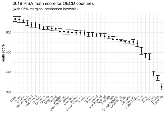
Figure 1: Raw math scores from 2018 PISA study.

Figure 1 shows the resulting graph. The function irank() can be used to produce integer ranks based on these math scores:

> math_rank <- irank(pisa$math_{s}core)>head(pisa[order(math_{r}ank),c("jurisdiction","math_{s}core","math_{s}e")])\par\addpenalty{\@beginparpenalty}\addvspace{\@topsep}\frenchspacing\hbox{\hbox to0.0pt{\kern 0.0pt\hss}\hbox to469.75499pt{\kern 0.0pt\hbox to469.75499pt{{\ \ \ jurisdiction\ math_score\ \ math_se}\hss}\hss}}{\penalty 150}\hbox to469.75499pt{\kern 0.0pt\hbox to469.75499pt{{19\ \ \ \ \ \ \ \ Japan\ \ \ 526.9733\ 2.471475}\hss}\hss}\penalty 0\hbox to469.75499pt{\kern 0.0pt\hbox to469.75499pt{{20\ \ \ \ \ \ \ \ Korea\ \ \ 525.9330\ 3.121394}\hss}\hss}\penalty 0\hbox to469.75499pt{\kern 0.0pt\hbox to469.75499pt{{9\ \ \ \ \ \ \ Estonia\ \ \ 523.4146\ 1.743602}\hss}\hss}\penalty 0\hbox to469.75499pt{\kern 0.0pt\hbox to469.75499pt{{25\ \ Netherlands\ \ \ 519.2310\ 2.632278}\hss}\hss}\penalty 0\hbox to469.75499pt{\kern 0.0pt\hbox to469.75499pt{{28\ \ \ \ \ \ \ Poland\ \ \ 515.6479\ 2.602085}\hss}\hss}\penalty 0\hbox to469.75499pt{\kern 0.0pt\hbox to469.75499pt{{34\ \ Switzerland\ \ \ 515.3147\ 2.908004}\hss}\hss}{\penalty 150}\hbox to469.75499pt{\kern 0.0pt\hbox to469.75499pt{{}\hss}\hss}\@endparenv\par Japanisrankedfirst(i.e.,best),Koreaisrankedsecondandsoon.Sincethemathscoresareestimatesofcountries\textquoteright trueachievements,theranksassignedtothesecountriesarealsoestimates,ratherthanthetrueranks.Justlikethetestscores,theranksthereforealsocontainstatisticaluncertainty.Variousfunctionsinthe\pkg{csranks}packageimplementmethodsforthequantificationofthisuncertainty,whichweredescribedinsection\ref{sec:methods}.\par$

4.1.2 Best populations

Suppose, that the researcher is interested in finding out which countries could be among the top-5 in terms of their true math score. One can answer this question by constructing the $\tau$-best confidence sets, described in section 2.2.3. In csranks, it is implemented in function cstaubest(). It requires as an argument an estimate of the covariance matrix of the test scores. In this example, it is assumed the estimates from the different countries are mutually independent, so the covariance matrix is diagonal. The function cstaubest() can then be used to compute a 95% confidence set for the top-5:

> math_cov_mat <- diag(pisa$math_{s}e^{2})>CS_{5}best<-cstaubest(pisa$math_score, math_cov_mat, tau = 5, coverage = 0.95) > pisa[CS_5best, "jurisdiction"]

 [1] Belgium     Canada      Denmark     Estonia     Finland     Japan [7] Korea       Netherlands Poland      Slovenia    Sweden      Switzerland37 Levels: Australia Austria Belgium Canada Chile Colombia ... United States

The confidence set contains 12 countries: with probability approximately 0.95, these 12 countries could all be among the top-5 according to their true math score. According to the estimated test scores, the countries Japan, Korea, Estonia, Netherlands, and Poland are the top-5 countries. However, due to the statistical uncertainty in the ranking, there is uncertainty about which countries are truly among the top-5.

4.1.3 Marginal confidence sets

Suppose that the researcher is interested in a single country, for example the United Kingdom. She would like to learn where its true ranking may lie. A marginal confidence set, described in section 2.2.1 and implemented in the function csranks() with parameter simul=FALSE, is a way to answer this question:

> uk_i <- which(pisa$jurisdiction=="UnitedKingdom")>CS_{m}arg<-csranks(pisa$math_score, math_cov_mat, simul=FALSE, > indices = uk_i, coverage=0.95) > CS_marg

$L[1] 7$rank[1] 13$U[1] 23attr(,"class")[1] "csranks"

CS_marg$L and CSmarg$U contain the lower and upper bounds of the confidence set for the rank of the United Kingdom.

Based on the estimated math scores, the United Kingdom is ranked at 13-th place. However, due to statistical uncertainty in the ranking, its true rank could be anywhere between 7 and 23, with probability approximately 95%.

4.1.4 Simultaneous confidence sets

Finally, suppose the researcher is interested in the entire ranking of countries. Simultaneous confidence sets (described in Section 2.2.2) for the ranks of all countries quantify the statistical uncertainty in the entire ranking. They are implemented in the function csranks() with parameter simul=TRUE:

> CS_simul <- csranks(pisa$math_{s}core,math_{c}ov_{m}at,+simul=TRUE,coverage=0.95)>gpl<-plot(CS_{s}imul,popnames=pisa$jurisdiction, + title="Ranking of OECD Countries by 2018 PISA Math Score", + subtitle="(with 95% simultaneous confidence sets)") > > ggsave("pisa_math.pdf", gpl, width=7, height=7)

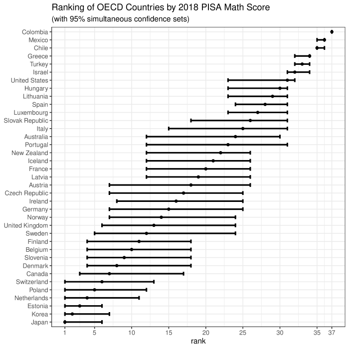
Figure 2: Simultaneous confidence sets for ranking according to PISA math test

The resulting graph is shown in Figure 2. The simultaneous confidence sets indicate substantial statistical uncertainty about ranks in the middle of the ranking. For instance, the confidence set for the true rank of Germany has a lower bound of 7 and and upper bound of 24. At the top and the bottom of the ranking, the statistical uncertainty is smaller. For instance, with approximately 95% probability, the true rank of Colombia is 37. The confidence sets for Mexico and Chile are also very tight and only contain two values.

4.2 Intergenerational Mobility

The following example illustrates how the csranks package can be used for estimation and inference in rank-rank regressions. These are commonly used for studying intergenerational mobility.

The dataset used in this example is the parent_child_income dataset that is part of the csranks package. It is a simulated dataset using a data-generating process calibrated to the National Longitudinal Survey of Youth 1979 from the U.S. Bureau of Labor Statistics. It includes data about parents’ (column c_faminc) and children’s (p_faminc) family income, as well as individual characteristics (gender and race: "hisp" (Hispanic), "black" or "neither").

First, we take a quick look at the dataset:

> data(parent_child_income) > head(parent_child_income)

   c_faminc  p_faminc gender    race1  78771.72 77127.484 female neither2  79268.33 62723.303 female neither3  45405.98 65751.340   male neither4  81951.64 58723.050   male neither5  88350.33  6381.047   male neither6 161331.33 40325.466 female neither>

A popular approach to measuring income mobility is to estimate a rank-rank regression of child’s income (c_faminc) on a constant and parent’s income (p_faminc). The lmranks() function implements this regression. The model can be specified through a formula in which the variables to be ranked are marked by r().

> lmr_model <- lmranks(r(c_faminc)   r(p_faminc), data=parent_child_income) > summary(lmr_model)

The number of residual degrees of freedom is not correct.Also, z-value, not t-value, since the distribution used for p-valuecalculation is standard normal.Call:lmranks(formula = r(c_faminc) ~ r(p_faminc), data = parent_child_income)Residuals:     Min       1Q   Median       3Q      Max-0.65601 -0.21986 -0.00376  0.22088  0.66495Coefficients:            Estimate Std. Error t value Pr(>|t|)(Intercept) 0.312311   0.007161   43.61   <2e-16 ***r(p_faminc) 0.375538   0.014319   26.23   <2e-16 ***---Signif. codes:  0 ‘***’ 0.001 ‘**’ 0.01 ‘*’ 0.05 ‘.’ 0.1 ‘ ’ 1Residual standard error: NA on 3892 degrees of freedom

This regression specification takes each child’s income, computes its rank among all children’s incomes, then takes each parent’s income and computes its rank among all parents’ incomes. Then the child’s rank is regressed on the parent’s rank using OLS. The summary() method computes standard errors, t-values and p-values according to the asymptotic theory developed in (Chetverikov:2023aa).

One can also run the rank-rank regression with additional covariates, e.g.:

> lmr_model_cov <- lmranks(r(c_faminc)   r(p_faminc) + gender + race, + data=parent_child_income) > summary(lmr_model_cov)

The number of residual degrees of freedom is not correct.Also, z-value, not t-value, since the distribution used for p-valuecalculation is standard normal.Call:lmranks(formula = r(c_faminc) ~ r(p_faminc) + gender + race,    data = parent_child_income)Residuals:     Min       1Q   Median       3Q      Max-0.66140 -0.20654 -0.00343  0.21421  0.72917Coefficients:             Estimate Std. Error t value Pr(>|t|)(Intercept)  0.299823   0.018155  16.514  < 2e-16 ***r(p_faminc)  0.323785   0.015123  21.411  < 2e-16 ***gendermale   0.010862   0.008484   1.280  0.20042raceblack   -0.088215   0.020910  -4.219 2.46e-05 ***raceneither  0.055726   0.018781   2.967  0.00301 **---Signif. codes:  0 ‘***’ 0.001 ‘**’ 0.01 ‘*’ 0.05 ‘.’ 0.1 ‘ ’ 1Residual standard error: NA on 3889 degrees of freedom

In some economic applications, it is desired to run rank-rank regressions separately in subgroups of the population, but compute the ranks in the whole population. For instance, we might want to estimate rank-rank regression slopes as measures of intergenerational mobility separately for males and females, but the ranking of children’s incomes is formed among all children (rather than form separate rankings for males and females).

Such regressions can be run using the lmranks() function with interaction notation:

> grouped_lmr_model <- lmranks(r(c_faminc)   r(p_faminc):gender, + data=parent_child_income) > summary(grouped_lmr_model)

The number of residual degrees of freedom is not correct.Also, z-value, not t-value, since the distribution used for p-valuecalculation is standard normal.Call:lmranks(formula = r(c_faminc) ~ r(p_faminc):gender, data = parent_child_income)Residuals:     Min       1Q   Median       3Q      Max-0.65016 -0.21977 -0.00308  0.21750  0.68833Coefficients:                         Estimate Std. Error t value Pr(>|t|)genderfemale              0.28796    0.01119   25.74   <2e-16 ***gendermale                0.33506    0.01107   30.27   <2e-16 ***r(p_faminc):genderfemale  0.40800    0.02046   19.94   <2e-16 ***r(p_faminc):gendermale    0.34516    0.02044   16.89   <2e-16 ***---Signif. codes:  0 ‘***’ 0.001 ‘**’ 0.01 ‘*’ 0.05 ‘.’ 0.1 ‘ ’ 1Residual standard error: NA on 3890 degrees of freedom

In this example, we have run a separate OLS regression of children’s ranks on parents’ ranks among the female and male children. However, incomes of children are ranked among all children and incomes of parents are ranked among all parents. The standard errors, t-values and p-values are implemented according to the asymptotic theory developed in (Chetverikov:2023aa), where it is shown that the asymptotic distribution of the estimators now need to not only account for the fact that ranks are estimated, but also for the fact that estimators are correlated across gender subgroups because they use the same estimated ranking.

One can also create more granular subgroups by interacting several characteristics such as gender and race:

> parent_child_income$subgroup<-interaction(parent_{c}hild_{i}ncome$gender, + parent_child_income$race)>gran{}_{g}rouped{}_{l}mr{}_{m}odel<-lmranks(r(c{}_{f}aminc)r(p{}_{f}aminc):subgroup,+data=parent{}_{c}hild{}_{i}ncome)>summary(gran{}_{g}rouped{}_{l}mr{}_{m}odel)\text{The number of residual degrees of freedom is not correct.}\text{Also, z-value, not t-value, since the distribution used for p-value}\text{calculation is standard normal.}\text{Call:}\text{lmranks(formula = r(c\_faminc) ~ r(p\_faminc):subgroup, data = parent\_child\_income)}\text{Residuals:}\text{ Min 1Q Median 3Q Max}\text{-0.65574 -0.20769 -0.00387 0.21297 0.73248}\text{Coefficients:}\text{ Estimate Std. Error t value Pr(>|t|)}\text{subgroupfemale.hisp 0.26280 0.03268 8.041 8.94e-16 ***}\text{subgroupmale.hisp 0.35313 0.04516 7.820 5.26e-15 ***}\text{subgroupfemale.black 0.19741 0.01968 10.031 < 2e-16 ***}\text{subgroupmale.black 0.26496 0.02702 9.805 < 2e-16 ***}\text{subgroupfemale.neither 0.35096 0.01525 23.006 < 2e-16 ***}\text{subgroupmale.neither 0.36603 0.01322 27.694 < 2e-16 ***}\text{r(p\_faminc):subgroupfemale.hisp 0.41733 0.07602 5.490 4.02e-08 ***}\text{r(p\_faminc):subgroupmale.hisp 0.21780 0.09697 2.246 0.024694 *}\text{r(p\_faminc):subgroupfemale.black 0.30798 0.05154 5.976 2.29e-09 ***}\text{r(p\_faminc):subgroupmale.black 0.25528 0.07234 3.529 0.000417 ***}\text{r(p\_faminc):subgroupfemale.neither 0.33908 0.02532 13.390 < 2e-16 ***}\text{r(p\_faminc):subgroupmale.neither 0.31818 0.02270 14.018 < 2e-16 ***}\text{—}\text{Signif. codes: 0 ‘***’ 0.001 ‘**’ 0.01 ‘*’ 0.05 ‘.’ 0.1 ‘ ’ 1}\text{Residual standard error: NA on 3882 degrees of freedom}Finally,wecomparetheconfidenceintervalsforrank-rankregressioncoefficientsproducedbylmranks()withthoseofthenaiveapproachwhichcomputestheranks,thenrunsaregressionofthechild{}^{\prime }sincomerankontheparent{}^{\prime }sincomerankusinglm(),andthenreportstheconfidenceintervalsbasedonthestandarderrorsfromlm().>\mathrm{\#}computechild{}^{\prime }srank>c{}_{f}aminc{}_{r}ank<-frank(parent{}_{c}hild{}_{i}ncomec{}_{f}aminc,omega=1,increasing=TRUE)>>\mathrm{\#}computeparent{}^{\prime }srank>p{}_{f}aminc{}_{r}ank<-frank(parent{}_{c}hild{}_{i}ncomep{}_{f}aminc,omega=1,increasing=TRUE)>>\mathrm{\#}naiverank-rankregression>lm{}_{m}odel<-lm(c{}_{f}aminc{}_{r}ankp{}_{f}aminc{}_{r}ank)>>\mathrm{\#}naivegroupedrank-rankregression>grouped{}_{l}m{}_{m}odel<-lm(c{}_{f}aminc{}_{r}ankp{}_{f}aminc{}_{r}ank:subgroup++subgroup-1,+data=parent{}_{c}hild{}_{i}ncome)>>\mathrm{\#}combineresults>theme{}_{s}et(theme{}_{m}inimal())>ci{}_{d}ata<-data.frame(estimate=coef(lmr{}_{m}odel),+parameter=c(\mathrm{"}Intercept\mathrm{"},\mathrm{"}slope\mathrm{"}),+group=\mathrm{"}Wholesample\mathrm{"},+method=\mathrm{"}csranks\mathrm{"},+lower=confint(lmr{}_{m}odel)[,1],+upper=confint(lmr{}_{m}odel)[,2])>ci{}_{d}ata<-rbind(ci{}_{d}ata,data.frame(+estimate=coef(gran{}_{g}rouped{}_{l}mr{}_{m}odel),+parameter=rep(c(\mathrm{"}Intercept\mathrm{"},\mathrm{"}slope\mathrm{"}),each=6),+group=rep(c(\mathrm{"}Hispanicfemale\mathrm{"},\mathrm{"}Hispanicmale\mathrm{"},\mathrm{"}Blackfemale\mathrm{"},+\mathrm{"}Blackmale\mathrm{"},\mathrm{"}Otherfemale\mathrm{"},\mathrm{"}Othermale\mathrm{"}),times=2),+method=\mathrm{"}csranks\mathrm{"},+lower=confint(gran{}_{g}rouped{}_{l}mr{}_{m}odel)[,1],+upper=confint(gran{}_{g}rouped{}_{l}mr{}_{m}odel)[,2]+))>ci{}_{d}ata<-rbind(ci{}_{d}ata,data.frame(+estimate=coef(lm{}_{m}odel),+parameter=c(\mathrm{"}Intercept\mathrm{"},\mathrm{"}slope\mathrm{"}),+group=\mathrm{"}Wholesample\mathrm{"},+method=\mathrm{"}naive\mathrm{"},+lower=confint(lm{}_{m}odel)[,1],+upper=confint(lm{}_{m}odel)[,2]+))>ci{}_{d}ata<-rbind(ci{}_{d}ata,data.frame(+estimate=coef(grouped{}_{l}m{}_{m}odel),+parameter=rep(c(\mathrm{"}Intercept\mathrm{"},\mathrm{"}slope\mathrm{"}),each=6),+group=rep(c(\mathrm{"}Hispanicfemale\mathrm{"},\mathrm{"}Hispanicmale\mathrm{"},\mathrm{"}Blackfemale\mathrm{"},+\mathrm{"}Blackmale\mathrm{"},\mathrm{"}Otherfemale\mathrm{"},\mathrm{"}Othermale\mathrm{"}),times=2),+method=\mathrm{"}naive\mathrm{"},+lower=confint(grouped{}_{l}m{}_{m}odel)[,1],+upper=confint(grouped{}_{l}m{}_{m}odel)[,2]+))>>\mathrm{\#}plotconfidencesets>gpl<-ggplot(ci{}_{d}ata,aes(y=estimate,x=group,ymin=lower,+ymax=upper,col=method,fill=method))++geom{}_{p}oint(position=position{}_{d}odge2(width=0.9))++geom{}_{e}rrorbar(position=position{}_{d}odge2(width=0.9))++geom{}_{h}line(aes(yintercept=estimate),+data=subset(ci{}_{d}ata,group==\mathrm{"}Wholesample\mathrm{"}),+linetype=\mathrm{"}dashed\mathrm{"},+col=\mathrm{"}gray\mathrm{"})++coord{}_{f}lip()++labs(title=\mathrm{"}95+inrank-rankregression\mathrm{"})++facet{}_{w}rap(parameter)>>ggsave(\mathrm{"}mobility.pdf\mathrm{"},gpl)Figure\text{<span class="ltx\_ref ltx\_missing\_label ltx\_font\_italic ltx\_ref\_self">LABEL:fig:rrreg-cis</span>}showstheresultinggraphcomparingtheconfidencesetsobtainedfromlmranks()(denotedby\mathrm{`}\mathrm{`}csranks{}^{\prime \prime })withthoseofthenaiveuseoflm()(denotedby\mathrm{`}\mathrm{`}naive{}^{\prime \prime })thatignorestheestimationerrorintheranks.\mathrm{`}\mathrm{`}Wholesample{}^{\prime \prime }referstotheconfidencesetsforinterceptandslopewhenarank-rankregressionisrunonthewholesample.Theotherrowsshowtheconfidencesetsfortheinterceptandslopeforeachgroupinthegroupedrank-rankregression.\text{Figure 3Figure 33Figure 33Confiden}$