LYT-NET: LIGHTWEIGHT YUV TRANSFORMER-BASED NETWORK FOR LOW-LIGHT IMAGE ENHANCEMENT

Abstract

In recent years, deep learning-based solutions have proven successful in the domains of image enhancement. This paper introduces LYT-Net, or Lightweight YUV Transformer-based Network, as a novel approach for low-light image enhancement. The proposed architecture, distinct from conventional Retinex-based models, leverages the YUV color space’s natural separation of luminance (Y) and chrominance (U and V) to simplify the intricate task of disentangling light and color information in images. By utilizing the strengths of transformers, known for their capability to capture long-range dependencies, LYT-Net ensures a comprehensive contextual understanding of the image while maintaining reduced model complexity. By employing a novel hybrid loss function, our proposed method achieves state-of-the-art results on low-light image enhancement datasets, all while being considerably more compact than its counterparts. The source code and pre-trained models are available at https://github.com/albrateanu/LYT-Net

1 Introduction

Low-light image enhancement (LLIE) is an important and challenging task in the realm of computer vision (CV). Capturing images in low-light conditions can significantly degrade their quality, resulting in a loss of details and contrast. This degradation not only leads to subjectively unpleasant visual experiences but also impairs the performance of many CV systems. The goal of LLIE is to improve visibility and contrast, while simultaneously restoring various distortions that are inherent in dark environments.

Low-light conditions refer to environmental scenarios where the level of illumination falls below the standard required for optimal visibility. However, in practical applications, it has so far been impossible to establish specific theoretical values that definitively characterize a low-light environment. As a result, there is no unified standard for identifying and quantifying what constitutes low-light conditions [1].

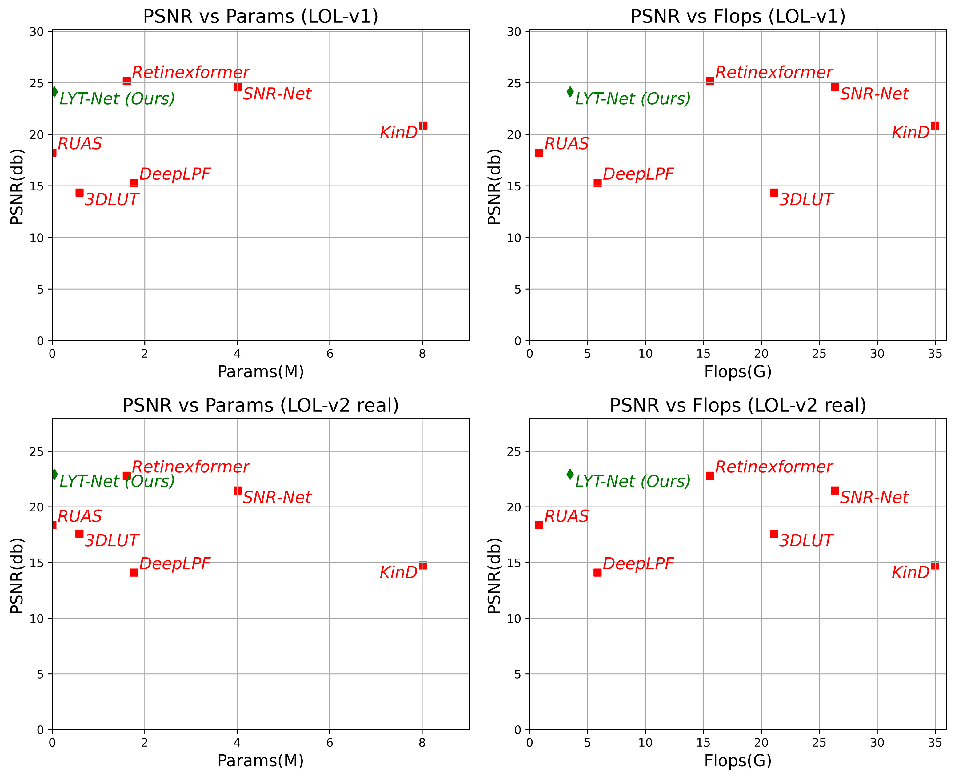
Figure 1: Proposed LYT-Net achieves SOTA performance on LLIE tasks while being computationally efficient. The metrics were evaluated on LOL dataset [2].

LLIE plays a significant role in various CV tasks such feature extraction [3, 4] or content-based recognition [5]. Moreover, it serves as a crucial step in more complex systems across diverse fields such as medical imaging [6], mobile remote sensing [7, 8], video monitoring systems [9], and so on.

LLIE solutions have advanced together with convolutional neural networks (CNN) and the proposed solutions fall into two main categories. The first involves using CNNs to directly map low-light images to their normal-light equivalents, a method that often overlooks human color perception and lacks theoretical interpretability. The second, inspired by Retinex theory, employs a more complex multi-stage training pipeline, utilizing different CNNs for tasks such as decomposing the color image, denoising the reflectance, and adjusting illumination. While this approach is more aligned with theoretical models, its complexity and requirement for multiple training stages presents notable challenges [10] .

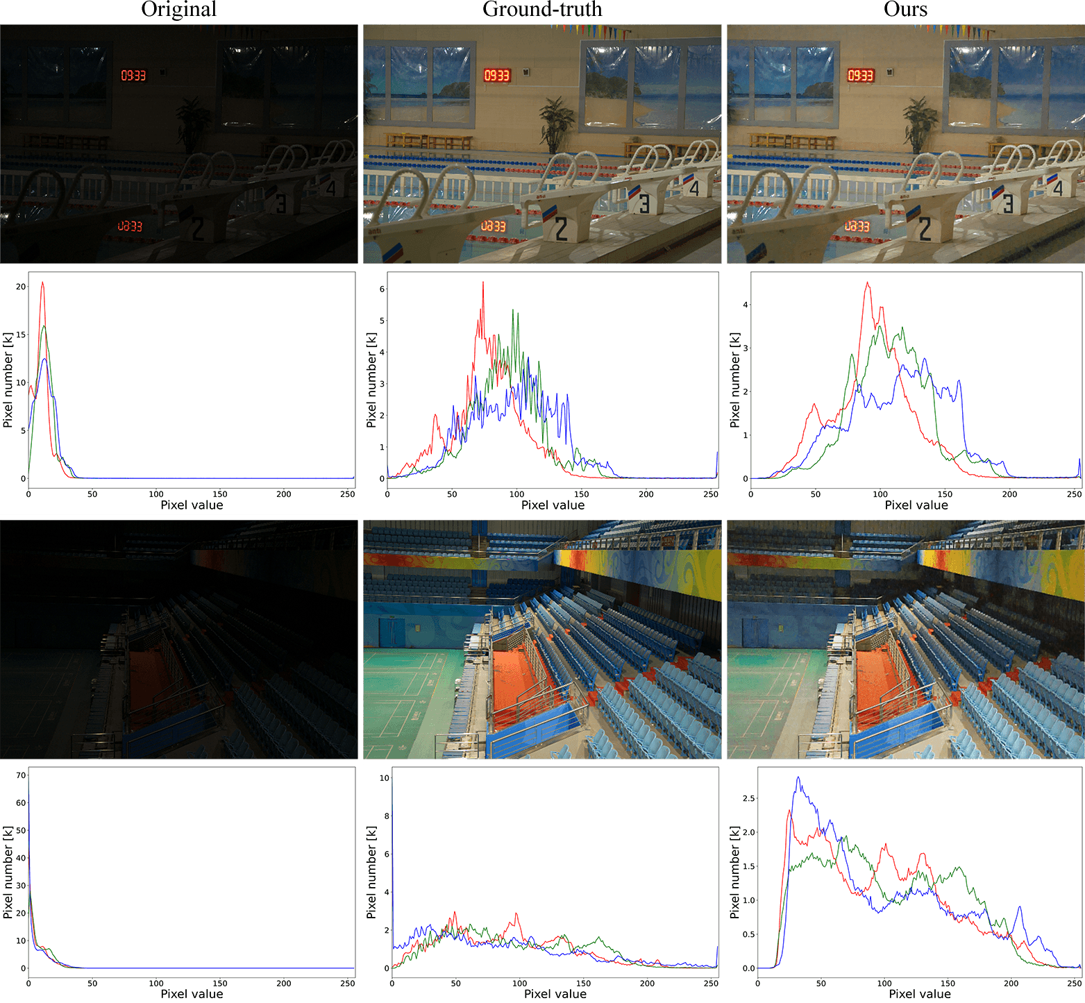
Figure 2: Visual results of LYT-Net on LOL dataset [11] . For a better understanding we added the histogram for each image.

In this paper, we propose a novel transformer-based approach, characterized by its low-weight design, that achieves state-of-the-art (SOTA) results in LLIE while maintaining computational efficiency. In Fig. 1 we present a comparative analysis of performance over complexity between SOTA methods evaluated using the LOL dataset [2]. For visual clarity, in the short comparison, we omitted models such as Restormer[12] and MIRNet[13] as they utilize considerably more parameters yet yield inferior results.

LYT-Net, demonstrates encouraging results, as illustrated in Fig. 2. Here, we have plotted the histogram of the predicted image to provide a clearer understanding of the model’s effect. Notably, the distribution in the histogram is smoother compared to the ground truth, which is a favorable outcome. This smoother distribution indicates that LYT-Net effectively enhances the image, balancing its tonal range and improving overall visual quality.

Our proposed model utilizes the YUV color space, which is particularly advantageous for LLIE due to its distinct separation of luminance (Y) and chrominance (U and V). By employing this color space, we can specifically target enhancements that can improve image visibility and detail in low-light conditions without adversely affecting the color information. Since human vision is more sensitive to changes in luminance, focusing on the Y channel leads to more natural and perceptually appealing enhancements.

The main contributions of our work can be summarized:

• LYT-Net, a lightweight model that employs the YUV color space to target enhancements. It utilizes a multi-headed self-attention scheme on the denoised luminance and chrominance layers, aiming for improved fusion at the end of the process.

• A hybrid loss function was designed, playing a critical role in the efficient training of our model and significantly contributing to its enhancement capabilities.

• Through quantitative and qualitative experiments, LYT-Net has demonstrated strong performance compared to SOTA methods on LOL datasets.

The paper is structured as follows: Section 1 provides an overview of the research and its importance. Section 2, "Related Work," aims to provide an overview on of the LLIE domain. In Section 3, "Proposed Method," we detail the proposed model and its key aspects, while in Section 4 we present the results on the LOL datasets. The paper concludes with Section 5, summarizing the findings and suggesting future research directions.

2 Related work

A significant number of papers have been published proposing various solutions for LLIE. One of the earliest methods proposed was histogram equalization and gamma correction [14], which relies on mapping gray levels in a manner that results in a uniform distribution.

A popular approach is based on cognitive methods that draw on Retinex theory [11], where a color image can be decomposed into two components: reflectance and illumination. The basic Retinex algorithm follows the core idea that an appropriate surround function is selected to determine the weighting of the pixel values in the neighborhood of the current pixel, hence the single-scale Retinex algorithm has emerged [15]. This was followed by the multiscale Retinex algorithms [16, 17].

With the rapid advancement of deep learning, CNNs have been extensively applied in LLIE. Following Retinex theory, the pioneering CNN-based method was Retinex-Net [2], which integrates Retinex decomposition with deep learning. Similarly, KinD [18] adopts the decomposition and adjustment paradigm, utilizing CNNs to learn the mapping in both decomposition and adjustment processes. A novel one-stage Retinex-based framework was proposed in Retinexformer [10], where the original Retinex model is enhanced by introducing perturbation terms to the reflectance and illumination to model corruptions. Diff-Retinex [19] proposes a generative framework to further compensate for content loss and color deviation caused by low light.

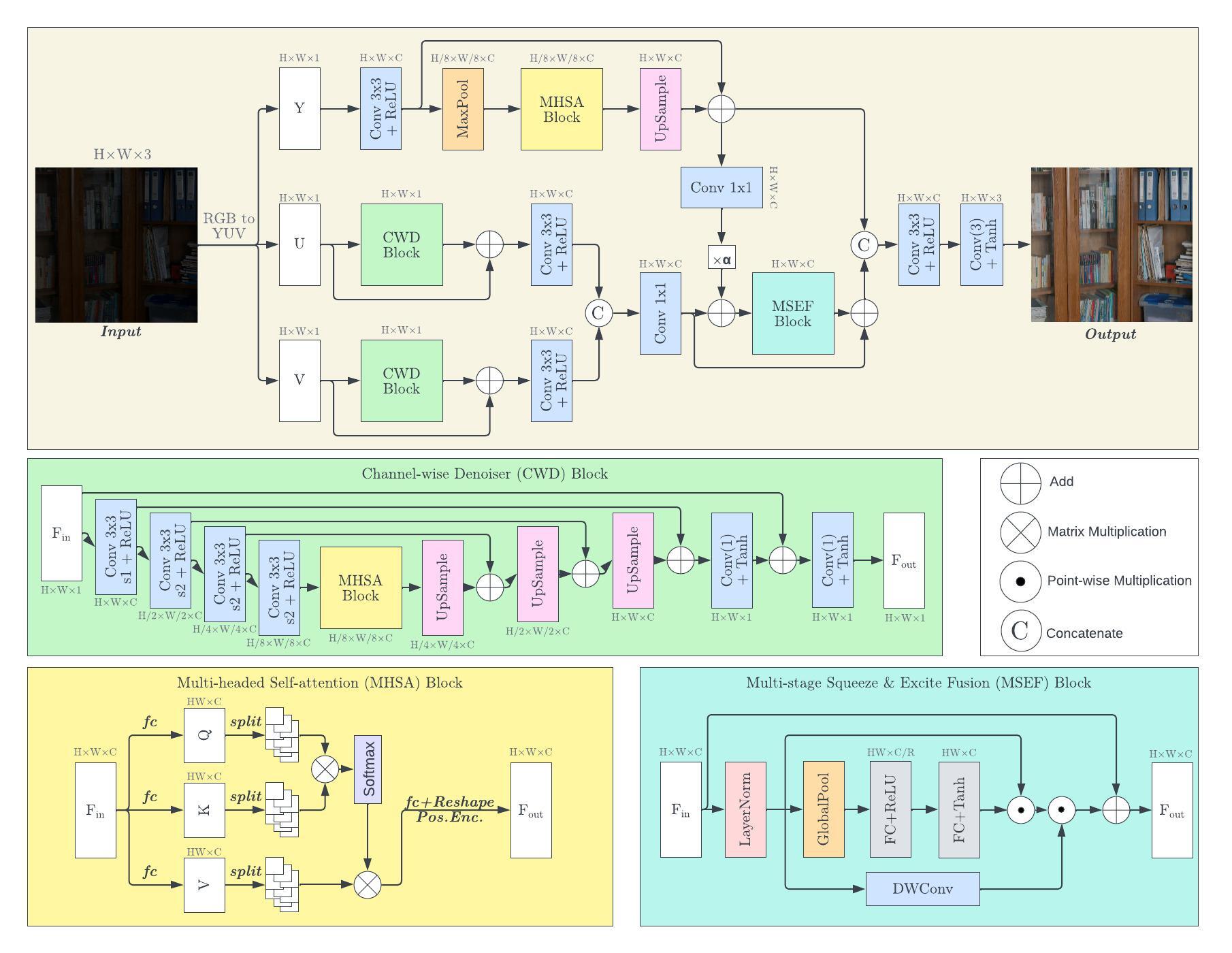
Figure 3: Overall framework of LYT-Net. The architecture consists of several detachable blocks like Channel-wise Denoiser (CWD), Multi-headed Self-Attention (MHSA), Multi-stage Squeeze and Excite Fusion (MSEF).

The development of Generative Adversarial Networks (GAN) [20] has offered a new perspective for LLIE, wherein low-light images are used as input to generate their normal-light equivalents. A notable example of this is EnlightenGAN [21], which uses a single generator model to directly convert low-light to normal-light versions, effectively employing both global and local discriminators in this transformation process. A distinct approach is presented in SNR-Net [22], which explores the relationship between signal and noise in the image space, utilizing the SNR for spatially varied enhancement.

3 PROPOSED METHOD

In Fig. 3 we illustrate the overall architecture of LYT-Net. As shown, the model consists of a main YUV decomposition to separate chrominance from luminance, followed by several layers and detachable blocks, like the Multi-headed Self-attention (MHSA) Block, Multi-stage Squeeze & Excite Fusion (MSEF) Block and Channel-wise Denoiser (CWD) Block. We adopt a dual-path approach, focusing on chrominance and luminance as separate entities, to help the model better understand the between difference illumination adjustment and corruption restoration.

As seen in Fig. 3, the model processes an input image in RGB format and converts it into YUV. Each channel is individually enhanced using a series of convolutional layers, pooling operations, and the MHSA mechanism. The luminance channel $Y$ undergoes convolution and pooling to extract features, which are then enhanced by the MHSA block. Chrominance channels $U$ and $V$ are processed through a CWD block to reduce noise while preserving details. The enhanced chrominance channels are then recombined and processed through the MSEF block. Ultimately, chrominance $UV$ and luminance $Y$ are concatenated and fed through a final set of convolutional layers to produce the output, yielding a high-quality enhanced image.

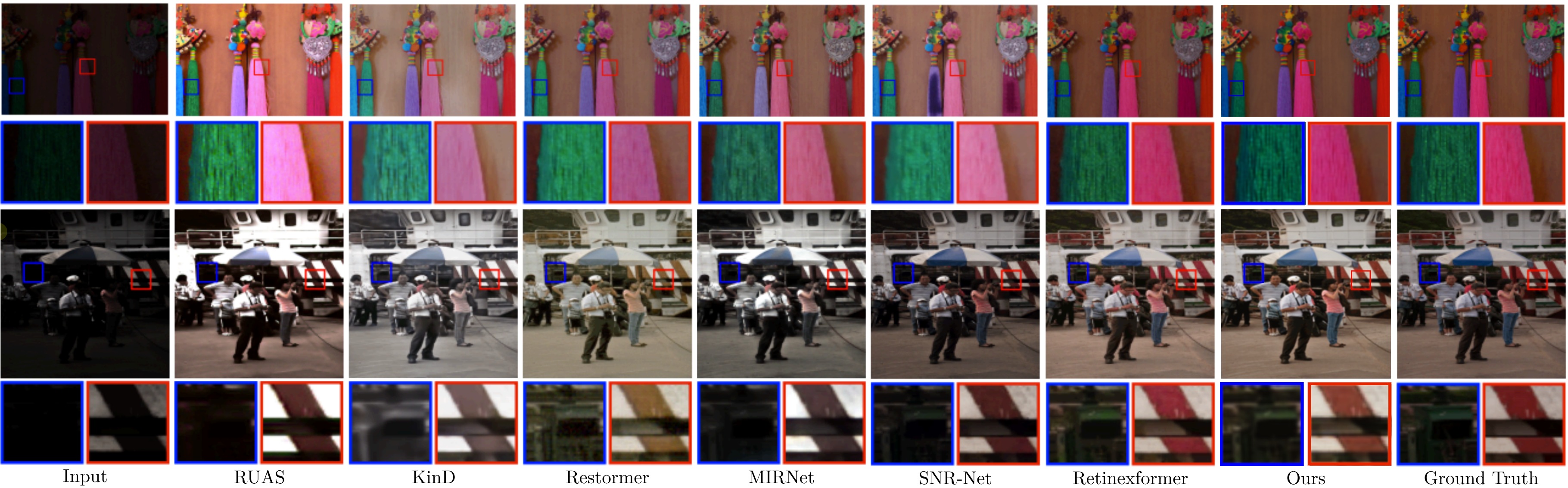
Figure 4: Qualitative comparison with SOTA LLIE methods on the LOL dataset. Zoom-in regions are used to illustrate differences.

3.1 Multi-headed Self-attention Block

In our simplified transformer architecture, we focus on the MHSA mechanism. The input feature $F_{\text{in}}\in\mathbb{R}^{H\times W\times C}$ is first linearly projected into query ($Q$), key ($K$), and value ($V$) components through bias-free fully connected layers.

$$Q=XW_{Q}^{T},K=XW_{K}^{T},V=XW_{V}^{T},Q,K,V\in\mathbb{R}^{HW\times C}$$ (1)

$$X=[X_{1},\ldots,X_{k}],X_{i}\in\mathbb{R}^{HW\times d_{k}},d_{k}=\frac{C}{k},i=\overline{1,k}$$ (2)

This projection is mathematically represented as in Eq. 3, where $W_{Q}$, $W_{K}$, and $W_{V}$ are the learnable parameters of the dense layers. The projected features are then reshaped into tokens $X$, and divided into $k$ heads as in Eq. 2. The self-attention mechanism, defined as in Eq. 3 is applied to each head, with the outputs concatenated and combined with positional encoding, resulting in the output tokens $X_{\text{out}}$, which are then reshaped to form the output feature $F_{\text{out}}\in\mathbb{R}^{H\times W\times C}$.

$$\text{Attention}(Q_{i},K_{i},V_{i})=V_{i}\odot\text{Softmax}(K_{i}^{T}Q_{i})$$ (3)

3.2 Multi-stage Squeeze & Excite Fusion Block

The MSEF Block enhances both spatial and channel-wise features of $F_{\text{in}}$. Initially, $F_{\text{in}}$ undergoes layer normalization, followed by global average pooling to capture global spatial context and a reduced fully-connected layer with ReLU activation, producing a reduced descriptor $S_{\text{reduced}}$, Eq. 4. This descriptor is then expanded back to the original dimensions through another fully-connected layer with Tanh activation, Eq. 5, resulting in $S_{\text{expanded}}$.

$$S_{\text{reduced}}=\text{ReLU}(W_{1}\cdot\text{GlobalPool}(\text{LayerNorm}(F_{\text{in}})))$$ (4)

$$S_{\text{expanded}}=\text{Tanh}(W_{2}\cdot S_{\text{reduced}})\cdot(\text{LayerNorm}(F_{\text{in}}))$$ (5)

A residual connection is added to the fused output to produce the final output feature map $F_{out}$, as in Eq. 6.

$$F_{\text{out}}=\text{DWConv}(\text{LayerNorm}(F_{\text{in}}))\cdot S_{\text{expanded}}+F_{\text{in}}$$ (6)

3.3 Channel-wise Denoiser Block

The CWD Block employs a U-shaped network with MHSA as the bottleneck, integrating convolutional and attention-based mechanisms. It includes multiple $conv3x3$ layers with varying strides and skip connections, facilitating detailed feature capture and denoising.

It consists of a series of four $conv3x3$. The first $conv3x3$ has strides of $1$ for feature extraction. The other three $conv3x3$ layers have strides of $2$, helping with capturing features at different scales. The integration of the attention bottleneck enables the model to capture long-range dependencies, proceeding to upsampling layers and skip connections to reconstruct and facilitate the recovery of spatial resolution.

Methods	Complexity		LOL-v1		LOL-v2-real		LOL-v2-syn
	FLOPS (G)	Params (M)	PSNR	SSIM	PSNR	SSIM	PSNR	SSIM
SID [23]	13.73	7.76	14.35	0.436	13.24	0.442	15.04	0.610
3DLUT [24]	0.075	0.59	14.35	0.445	17.59	0.721	18.04	0.800
DeepUPE [25]	21.10	1.02	14.38	0.446	13.27	0.452	15.08	0.623
DeepLPF [26]	5.86	1.77	15.28	0.473	14.10	0.480	16.02	0.587
UFormer [27]	12.00	5.29	16.36	0.771	18.82	0.771	19.66	0.871
RetinexNet [2]	587.47	0.84	16.77	0.560	15.47	0.567	17.13	0.798
Sparse [28]	53.26	2.33	17.20	0.640	20.06	0.816	22.05	0.905
EnGAN [21]	61.01	114.35	17.48	0.650	18.23	0.617	16.57	0.734
RUAS [29]	0.83	0.003	18.23	0.720	18.37	0.723	16.55	0.652
FIDE [30]	28.51	8.62	18.27	0.665	16.85	0.678	15.20	0.612
KinD [18]	34.99	8.02	20.86	0.790	14.74	0.641	13.29	0.578
Restormer [12]	144.25	26.13	22.43	0.823	19.94	0.827	21.41	0.830
MIRNet [13]	785	31.76	24.14	0.830	20.02	0.820	21.94	0.876
SNR-Net [22]	26.35	4.01	24.61	0.842	21.48	0.849	24.14	0.928
Retinexformer [10]	15.57	1.61	25.16	0.845	22.80	0.840	25.67	0.930
LYT-Net	3.49	0.045	24.13	0.844	22.93	0.840	23.33	0.905

Table 1: Quantitative results on LOL datasets and method complexity. Best results are in red, second best are in blue, while third best are in green.

3.4 Loss Function

In our approach, a hybrid loss function plays a pivotal role in training our model effectively. The hybrid loss $L$ is formulated as in Eq. 3.4, where $\alpha_{1}$ to $\alpha_{6}$ are hyperparameters used to balance each constituent loss function.

$$L= \alpha_{1}L_{\text{S}}+\alpha_{2}L_{\text{Perc}}+\alpha_{3}L_{\text{Hist}}$$

$$+\alpha_{4}L_{\text{PSNR}}+\alpha_{5}L_{\text{Color}}+\alpha_{6}L_{\text{MS-SSIM}},$$ (7)

The Smooth L1 loss $L_{\text{S}}$, a robust variant of the L1 loss less sensitive to outliers, defined in Eq. 8.

$$L_{\text{S}}=\begin{cases}0.5\cdot(y_{\text{true}}-y_{\text{pred}})^{2}&,\text{if }|y_{\text{true}}-y_{\text{pred}}|<1\\ |y_{\text{true}}-y_{\text{pred}}|-0.5&,\text{otherwise}\end{cases}$$ (8)

Perceptual loss $L_{\text{Perc}}$, Eq. 9, provides high-level feature supervision. $N$ is the total number of features, $VGG_{i}$ is the output of the $i$-th layer in a pre-trained VGG network, and $C_{i},H_{i},W_{i}$ are dimensions of the feature map.

$$L_{\text{Perc}}=\frac{1}{N}\sum_{i=1}^{N}\frac{1}{C_{i}H_{i}W_{i}}\left\|VGG_{i}(y_{pred})-VGG_{i}(y_{true})\right\|_{2}^{2},$$ (9)

Histogram loss aligns the distribution of pixel intensities true and predicted images. $\text{Hist}(y,b)$ is the count of pixels in the $b$-th bin of the histogram for image $y$. $B$ is the total number of bins in the histogram. $L_{\text{H}}$ is given by Eq. 10.

$$L_{\text{Hist}}=\sum_{b=1}^{B}\left|\frac{\text{Hist}(y_{\text{true}},b)}{\sum_{b=1}^{B}\text{Hist}(y_{\text{true}},b)}-\frac{\text{Hist}(y_{\text{pred}},b)}{\sum_{b=1}^{B}\text{Hist}(y_{\text{pred}},b)}\right|,$$ (10)

PSNR is a common metric for image quality assessment. $L_{\text{PSNR}}$ is defined as in Eq. 11.

$$L_{\text{PSNR}}=40.0-10\log_{10}\left(\frac{\text{MAX}_{I}^{2}}{\text{MSE}(y_{\text{true}},y_{\text{pred}})}\right),$$ (11)

Color loss ensures color fidelity between the generated and target images. $\bar{y}_{c}$ represents the mean pixel values accros height $H$ and width $W$ for channel $c$. $L_{\text{Color}}$ is defined in Eq. 12.

$$L_{\text{Color}}=\sum_{c=1}^{C}\left|\bar{y}_{\text{true},c}-\bar{y}_{\text{pred},c}\right|,$$ (12)

Multiscale Structural Similarity Index Measure (SSIM) loss $L_{\text{MS-SSIM}}$, which evaluates structural similarity at multiple scales, is vital for maintaining the structural integrity of the images is described in Eq. 13.

$${}L_{\text{MS-SSIM}}=1-\prod_{m=1}^{M} \left(\frac{2\mu_{H}\mu_{G}+C_{1}}{\mu_{H}^{2}+\mu_{G}^{2}+C_{1}}\right)^{\beta_{m}}$$ (13)

$$\times\left(\frac{2\sigma_{HG}+C_{2}}{\sigma_{H}^{2}+\sigma_{G}^{2}+C_{2}}\right)^{\gamma_{m}},$$

The purpose of our hybrid loss is to account for outlier values (by $L_{\text{S}}$), human-like image perception (by $L_{\text{Perc}}$), statistical information (by $L_{\text{Color}}$ and $L_{\text{Hist}}$), noise control (by $L_{\text{PSNR}}$), and qualitative fidelity (by $L_{\text{MS-SSIM}}$).

4 EXPERIMENTS AND RESULTS

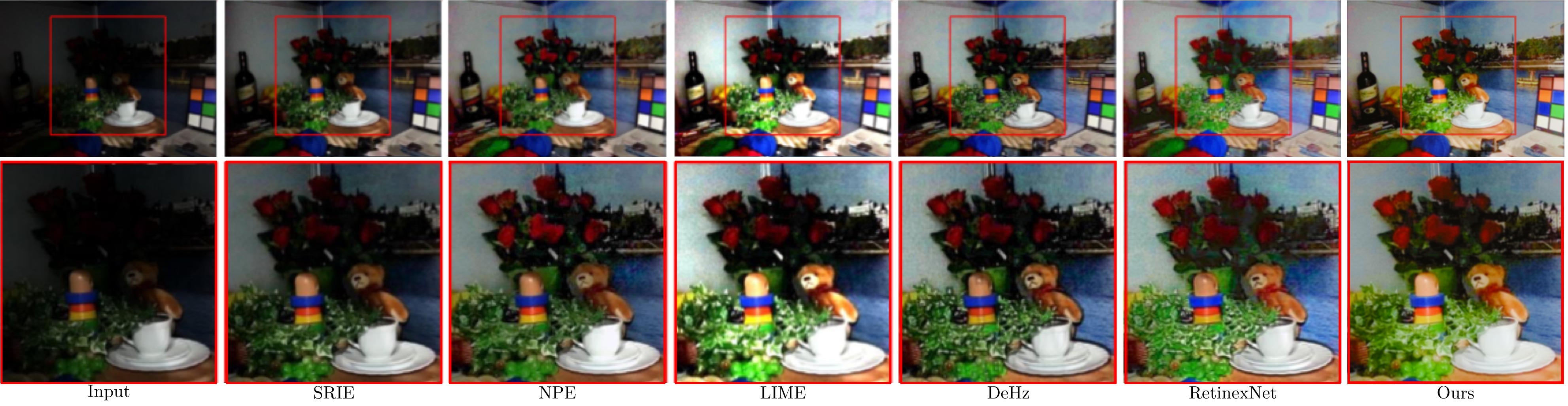
Figure 5: Qualitative comparison with SOTA LLIE methods on LIME dataset. Zoom-in regions are used to illustrate differences.

4.1 Implementation specifics

The implementation of LYT-Net utilizes the Tensorflow framework. The ADAM Optimizer ($\beta_{1}=0.9$ and $\beta_{2}=0.999$), serves as the optimizer for $1000$ epochs. It starts with an initial learning rate of $2\times 10^{-4}$ and undergoes a gradual reduction to $1\times 10^{-6}$ through the cosine annealing scheme. This strategy contributes to enhanced optimization convergence and prevents potential learning blockages caused by local minima.

LYT-Net is trained and evaluated on versions of the LOL dataset: v1, v2-real, and v2-synthetic. The training/testing splits corresponding to each version are 485:15 for LOL-v1, 689:100 for LOL-v2-real, and 900:100 for LOL-v2-synthetic.

Training pairs are passed through a random jittering process which undergoes a random cropping process to $256\times 256$ and other augmentations such as random flipping/rotation to avoid overfitting. Pairs are subsequently fed into the training process with a batch size of $1$. Finally, the evaluation metrics encompass PSNR and SSIM.

4.2 Quantitative results

The proposed method is evaluated against SOTA LLIE techniques, as shown in Table 1. This comparison focuses on two crucial aspects: the quantitative performance on the designated datasets (LOL-v1, LOL-v2-real, and LOL-v2-synthetic) and complexity.

As indicated in Table 1, our model, LYT-Net, consistently achieves top three scores across all variants of the LOL dataset. In terms of complexity, LYT-Net is notably efficient, utilizing just $3.49G$ FLOPS (Floating Point Operations Per Second) and a remarkably low number of parameters, $0.045M$. This efficiency significantly reduces computational requirements compared to other SOTA methods. This balance of performance and efficiency gives us confidence in stating that our method yields significantly good results.

In terms of complexity, LYT-Net ranks third best. However, when compared to methods like 3DLUT or RUAS, which have lower complexities, the quantitative results highlights that LYT-Net delivers improved outcomes.

Comparing to models such as SNR-Net, Retinexformer, or MIRNet, LYT-Net stands out for its competitive performance coupled with substantially lower computational cost.

4.3 Qualitative Results

The proposed method is evaluated qualitative against SOTA LLIE techniques in Fig. 4 on LOL dataset, and in Fig. 5 on LIME [31]. It’s noteworthy that previous methods have displayed certain limitations. For instance, KiND and Restormer, as shown in Fig. 4, suffer from color distortion problems.

Additionally, several methods tend to produce over- or under-exposed areas, compromising image contrast in the process of enhancing luminance. This issue is evident with algorithms like RUAS, MIRNet, and SNR-Net in Fig. 4. The same problem is observable in Fig. 5 with other algorithms such as SRIE [32], DeHz [33] and NPE [34], where attempts to illuminate the image result in a loss of contrast. These observations highlight the challenges in balancing exposure and color fidelity in LLIE, areas where LYT-Net aims to offer improvements.

5 CONCLUSION AND FUTURE WORKS

The data presented in these work highlights LYT-Net’s ability to deliver high-quality image enhancement with minimal computational resources. Its performance is comparable to, and in some cases surpasses, heavier and more complex models, making it an attractive solution for applications where computational efficiency is as crucial.

In summary, LYT-Net distinguishes itself by offering a highly effective balance between performance and efficiency, achieving top-tier results on standard benchmarks while maintaining ultra-lightweight properties.

Looking ahead, we plan to further evaluate our model on larger datasets and incorporate user feedback to enhance our benchmarking. Given LYT-Net’s low complexity, we also foresee its potential integration with sensor systems, expanding its applicability in real-world scenarios.

References

- [1] W. Wang, X. Wu, X. Yuan, and Z. Gao, “An experiment-based review of low-light image enhancement methods,” Ieee Access, vol. 8, pp. 87 884–87 917, 2020.
- [2] C. Wei, W. Wang, W. Yang, and J. Liu, “Deep retinex decomposition for low-light enhancement,” in Proceedings of the British Machine Vision Conference (BMVC), 2018.
- [3] C. Orhei and R. Vasiu, “An analysis of extended and dilated filters in sharpening algorithms,” IEEE Access, 2023.
- [4] C. Orhei, V. Bogdan, C. Bonchis, and R. Vasiu, “Dilated filters for edge-detection algorithms,” Applied Sciences, vol. 11, no. 22, p. 10716, 2021.
- [5] C.-C. Orhei, “Urban landmark detection using computer vision,” Ph.D. dissertation, Universitatea Politehnica Timişoara, 2022.
- [6] C. D. Căleanu, C. L. Sîrbu, and G. Simion, “Deep neural architectures for contrast enhanced ultrasound (CEUS) focal liver lesions automated diagnosis,” vol. 21, no. 12. MDPI, 2021, p. 4126.
- [7] S. Vert, D. Andone, A. Ternauciuc, V. Mihaescu, O. Rotaru, M. Mocofan, C. Orhei, and R. Vasiu, “User evaluation of a multi-platform digital storytelling concept for cultural heritage,” Mathematics, vol. 9, no. 21, p. 2678, 2021.
- [8] C. Orhei, L. Radu, M. Mocofan, S. Vert, and R. Vasiu, “Urban landmark detection using A-KAZE features and vector of aggregated local descriptors,” in 2022 International Symposium on Electronics and Telecommunications (ISETC). IEEE, 2022, pp. 1–4.
- [9] A. Avram, I. Porobic, and P. Papazian, “An overview of intelligent surveillance systems development,” in 2018 International Symposium on Electronics and Telecommunications (ISETC), 2018, pp. 1–6.
- [10] S. Yang, D. Zhou, J. Cao, and Y. Guo, “Rethinking low-light enhancement via transformer-gan,” IEEE Signal Processing Letters, vol. 29, pp. 1082–1086, 2022.
- [11] E. H. Land, “The retinex theory of color vision,” Scientific american, vol. 237, no. 6, pp. 108–129, 1977.
- [12] S. W. Zamir, A. Arora, S. Khan, M. Hayat, F. S. Khan, and M.-H. Yang, “Restormer: Efficient transformer for high-resolution image restoration,” in Proceedings of the IEEE/CVF conference on computer vision and pattern recognition, 2022, pp. 5728–5739.
- [13] S. W. Zamir, A. Arora, S. Khan, M. Hayat, F. S. Khan, M.-H. Yang, and L. Shao, “Learning enriched features for real image restoration and enhancement,” in Computer Vision–ECCV 2020: 16th European Conference, Glasgow, UK, August 23–28, 2020, Proceedings, Part XXV 16. Springer, 2020, pp. 492–511.
- [14] W. Wang, X. Wu, X. Yuan, and Z. Gao, “An experiment-based review of low-light image enhancement methods,” Ieee Access, vol. 8, pp. 87 884–87 917, 2020.
- [15] D. J. Jobson, Z.-u. Rahman, and G. A. Woodell, “Properties and performance of a center/surround retinex,” IEEE transactions on image processing, vol. 6, no. 3, pp. 451–462, 1997.
- [16] Z.-u. Rahman, D. J. Jobson, and G. A. Woodell, “Multi-scale retinex for color image enhancement,” in Proceedings of 3rd IEEE international conference on image processing, vol. 3. IEEE, 1996, pp. 1003–1006.
- [17] D. J. Jobson, Z.-u. Rahman, and G. A. Woodell, “A multiscale retinex for bridging the gap between color images and the human observation of scenes,” IEEE Transactions on Image processing, vol. 6, no. 7, pp. 965–976, 1997.
- [18] Y. Zhang, J. Zhang, and X. Guo, “Kindling the darkness: A practical low-light image enhancer,” in Proceedings of the 27th ACM international conference on multimedia, 2019, pp. 1632–1640.
- [19] X. Yi, H. Xu, H. Zhang, L. Tang, and J. Ma, “Diff-retinex: Rethinking low-light image enhancement with a generative diffusion model,” in Proceedings of the IEEE/CVF International Conference on Computer Vision, 2023, pp. 12 302–12 311.
- [20] L. Zhu, Y. Chen, P. Ghamisi, and J. A. Benediktsson, “Generative adversarial networks for hyperspectral image classification,” IEEE Transactions on Geoscience and Remote Sensing, vol. 56, no. 9, pp. 5046–5063, 2018.
- [21] Y. Jiang, X. Gong, D. Liu, Y. Cheng, C. Fang, X. Shen, J. Yang, P. Zhou, and Z. Wang, “Enlightengan: Deep light enhancement without paired supervision,” IEEE transactions on image processing, vol. 30, pp. 2340–2349, 2021.
- [22] X. Xu, R. Wang, C.-W. Fu, and J. Jia, “SNR-aware low-light image enhancement,” in Proceedings of the IEEE/CVF conference on computer vision and pattern recognition, 2022, pp. 17 714–17 724.
- [23] C. Chen, Q. Chen, M. N. Do, and V. Koltun, “Seeing motion in the dark,” in Proceedings of the IEEE/CVF International conference on computer vision, 2019, pp. 3185–3194.
- [24] H. Zeng, J. Cai, L. Li, Z. Cao, and L. Zhang, “Learning image-adaptive 3d lookup tables for high performance photo enhancement in real-time,” IEEE Transactions on Pattern Analysis and Machine Intelligence, vol. 44, no. 4, pp. 2058–2073, 2020.
- [25] R. Wang, Q. Zhang, C.-W. Fu, X. Shen, W.-S. Zheng, and J. Jia, “Underexposed photo enhancement using deep illumination estimation,” in Proceedings of the IEEE/CVF conference on computer vision and pattern recognition, 2019, pp. 6849–6857.
- [26] S. Moran, P. Marza, S. McDonagh, S. Parisot, and G. Slabaugh, “DeepLPF: Deep local parametric filters for image enhancement,” in Proceedings of the IEEE/CVF conference on computer vision and pattern recognition, 2020, pp. 12 826–12 835.
- [27] Z. Wang, X. Cun, J. Bao, W. Zhou, J. Liu, and H. Li, “Uformer: A general u-shaped transformer for image restoration,” in Proceedings of the IEEE/CVF conference on computer vision and pattern recognition, 2022, pp. 17 683–17 693.
- [28] W. Yang, W. Wang, H. Huang, S. Wang, and J. Liu, “Sparse gradient regularized deep retinex network for robust low-light image enhancement,” IEEE Transactions on Image Processing, vol. 30, pp. 2072–2086, 2021.
- [29] R. Liu, L. Ma, J. Zhang, X. Fan, and Z. Luo, “Retinex-inspired unrolling with cooperative prior architecture search for low-light image enhancement,” in Proceedings of the IEEE/CVF Conference on Computer Vision and Pattern Recognition, 2021, pp. 10 561–10 570.
- [30] K. Xu, X. Yang, B. Yin, and R. W. Lau, “Learning to restore low-light images via decomposition-and-enhancement,” in Proceedings of the IEEE/CVF conference on computer vision and pattern recognition, 2020, pp. 2281–2290.
- [31] X. Guo, Y. Li, and H. Ling, “Lime: Low-light image enhancement via illumination map estimation,” IEEE Transactions on image processing, vol. 26, no. 2, pp. 982–993, 2016.
- [32] X. Fu, D. Zeng, Y. Huang, Y. Liao, X. Ding, and J. Paisley, “A fusion-based enhancing method for weakly illuminated images,” Signal Processing, vol. 129, pp. 82–96, 2016.
- [33] X. Dong, Y. Pang, and J. Wen, “Fast efficient algorithm for enhancement of low lighting video,” in ACM SIGGRAPH 2010 Posters, 2010, pp. 1–1.
- [34] S. Wang, J. Zheng, H.-M. Hu, and B. Li, “Naturalness preserved enhancement algorithm for non-uniform illumination images,” IEEE transactions on image processing, vol. 22, no. 9, pp. 3538–3548, 2013.