Predictive linear seesaw model with family symmetry.
Abstract
We consider a model that accounts for the smallness of neutrino masses through the linear seesaw mechanism and employs a family symmetry to address the flavour problem. The model is predictive in the leptonic sector and faces constraints from Lepton Flavour Violation processes, namely , which indicate a range for the Right-Handed neutrino mass.
pacs:
12.60.Cn,12.60.Fr,12.15.Lk,14.60.PqI Introduction
The observation of the Higgs boson at the LHC has further confirmed the Standard Model (SM). However some beyond SM physics is needed due to the observed neutrino mixing. Further, in the SM, the fermion masses and mixings arise from the Yukawa couplings of the fermions to the Higgs, which are numerous, hierarchical, and with a strikingly different pattern between quark mixing and the mixing observed for the leptons. This is often referred to as the flavour problem, and a possible solution is that family symmetries are added, together with some type of seesaw mechanism. With the family symmetry, the Yukawa couplings to the SM Higgs are then obtained from the pattern of family symmetry breaking.
A popular family symmetry is . Its main advantage is that it is a small symmetry with a triplet and anti-triplet representation. The typical pattern of symmetry breaking that emerges from is also able to naturally account for the observed leptonic mixing in a large class of models, and it also has very appealing interplay with CP symmetries. [1, 2, 3, 4, 5, 6, 7, 8, 9, 10, 11, 12, 13, 14, 15, 16, 17, 18, 19, 20, 21, 22, 23, 24, 25, 26, 27, 28, 29, 30, 31, 32, 33, 34].
In this paper we consider a simple model that employs a family symmetry and linear seesaw mechanism to generate the tiny masses for the active neutrinos.
In order to obtain a viable model, we need to break with multiple fields [8, 12, 14] (this is typical of discrete symmetries with triplets, see [35]).
This model of leptonic mixing we do not address the quarks, which can be fitted as in the SM.
II The model
We consider a supersymmetric model where the full symmetry features a two-step spontaneous breaking pattern:
| (1) |
It is assumed that the discrete groups are spontaneously broken at an energy scale much larger than the electroweak symmetry breaking scale GeV. In our supersymmetric model, the scalar sector of MSSM is enlarged by several gauge singlet scalar fields, whereas the fermion sector is augmented by two heavy RH Majorana neutrinos, i.e., and . Such extension of the particle spectrum is necessary for the implementation of the linear seesaw mechanism that yields the tiny active neutrino masses. The assignments of fermions and scalars in our model are shown in Table 1. In our proposed model, the symmetry allows that only one scalar triplet participates in the charged lepton Yukawa interactions, thus yielding a diagonal charged lepton mass matrix, thanks to the vacuum expectation value (VEV) configuration of to be shown below. Furthermore, symmetry separates the scalar triplets and participating in the neutrino Yukawa interactions with with the triplet appearing in the Yukawa terms for charged leptons and right handed Majorana neutrino . The symmetry, which is spontaneously broken by the VEV of the scalar singlet , is crucial for the implementation of the Froggat-Nielsen mechanism that yields the observed patttern of SM charged lepton masses. Furthermore, the discrete flavor symmetry is necessary to get a predictive lepton sector through the following VEV configurations for the triplets scalars:
| (2) |
where the VEV pattern of yields a diagonal matrix for SM charged leptons, thus implying that the leptonic mixing entirely arises from the neutrino sector. These special VEV patterns are the motivation for considering flavored SUSY models, as such configurations can arise from the F-term alignment mechanism [19] or D-term alignment mechanism [2]. This is in contrast with the somewhat generic VEV used in [25, 30].
Since the observed pattern of SM charged lepton masses arises from the spontaneous breaking of the discrete symmetry, we set the VEVs of the different gauge singlet scalars as follows:
| (3) |
where , being the reactor mixing angle, whereas is the model cutoff, which can be interpreted as the scale of the UV completion of the model, e.g. the masses of the Froggatt-Nielsen messenger fields.
With the above mentioned particle content and symmetries, the following leptonic Yukawa interactions arise:
| (4) |
| (5) | |||||
| 0 | 0 | 0 | 0 | x | |||||||||||
| 0 | 8 | 4 | 2 | 0 | 0 | 0 | 0 | -1 | 0 | 0 | 0 | 0 | 0 | 0 |
III Lepton masses and mixings
After the spontaneus breaking of the SM gauge symmetry and the discrete group, we find that the SM charged lepton mass matrix is diagonal with the charged lepton masses given by:
| (6) |
where , and are real dimensionless parameters and we have assumed that , being GeV the electroweak symmetry breaking scale.
Furthermore, the neutrino Yukawa interactions yield the following neutrino mass terms:
| (7) |
where the neutrino mass matrix is given by:
| (8) |
and the submatrices and have the following structure:
| (9) |
The active light neutrino masses are generated from linear seesaw mechanism, and the physical low energy neutrino mass matrix is given by:
| (13) |
Furthermore, the masses for the physical heavy pseudo-Dirac neutrinos are given by:
| (14) | |||||
| (15) |
| Observable | ||||||
|---|---|---|---|---|---|---|
| Experimental value | ||||||
| Best-fit model |
The mass matrix of light active neutrinos from Eq. (13) is consistent with the experimental data of neutrino oscillations, reproducing the neutrino mass squared difference, the mixing angles and the leptonic CP violating phase. The result of our fit can be seen in the table 2 where it is observed that the best-fit point of the model is within the experimental range of for each observable. This adjustment of the parameters that reproduce the neutrino sector was obtained by minimizing function, which is defined as,
| (16) |
where is the difference of the square of the neutrino masses (with ), is the sine function of the mixing angles (with ) and is the CP violation phase. The superscripts represent the experimental (“exp”) and theoretical (“th”) values and the are the experimental errors. Therefore, the minimization of gives us the following value,
| (17) |
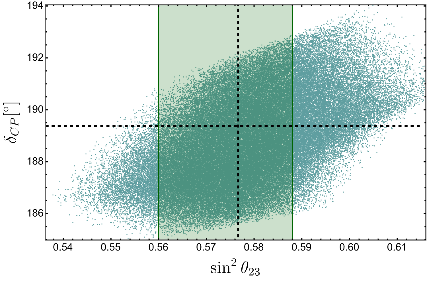
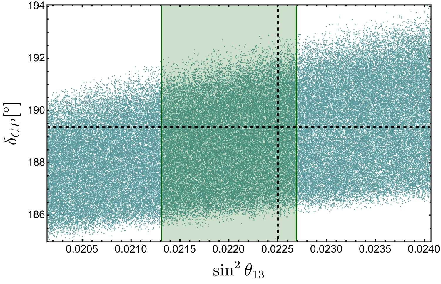
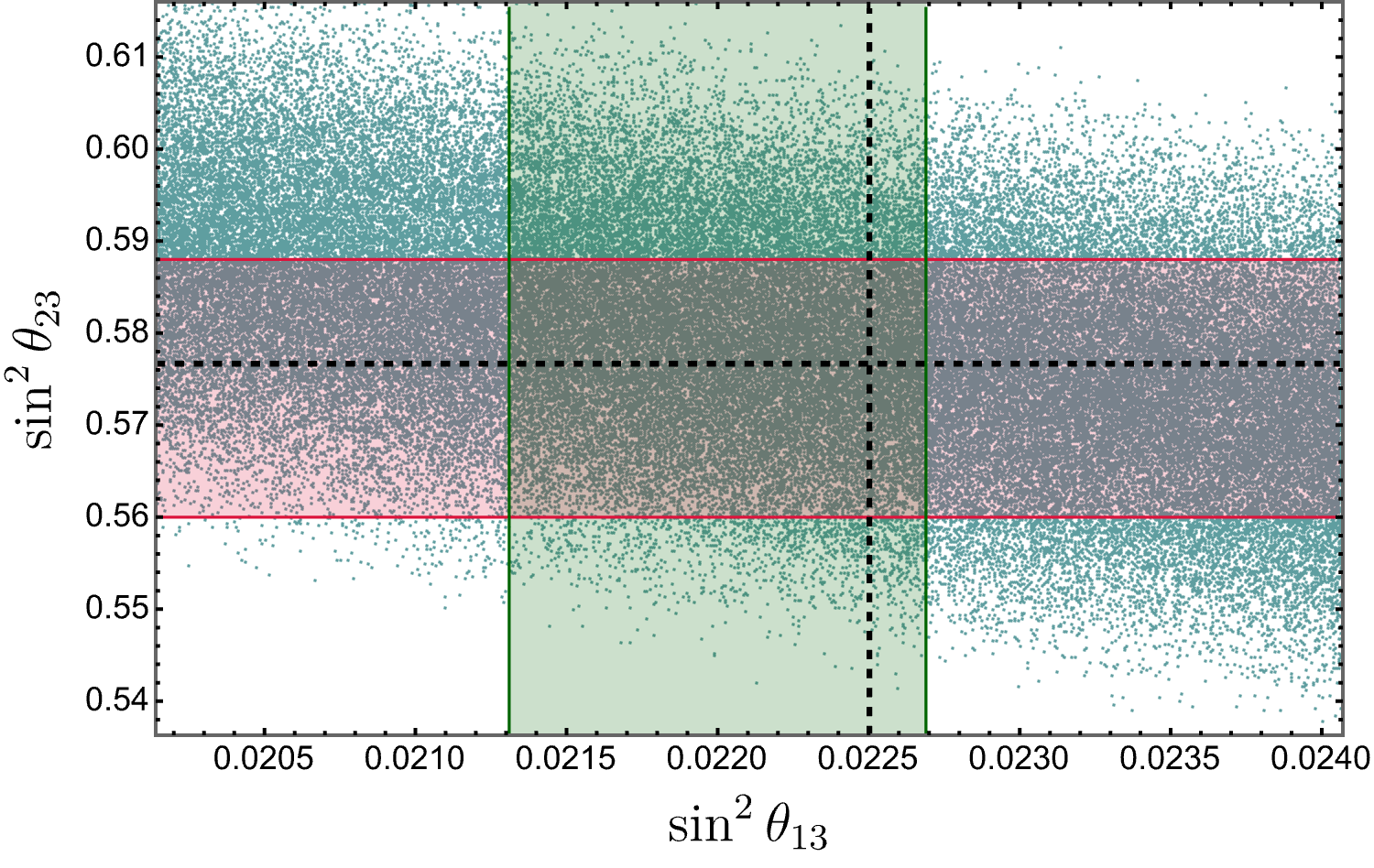
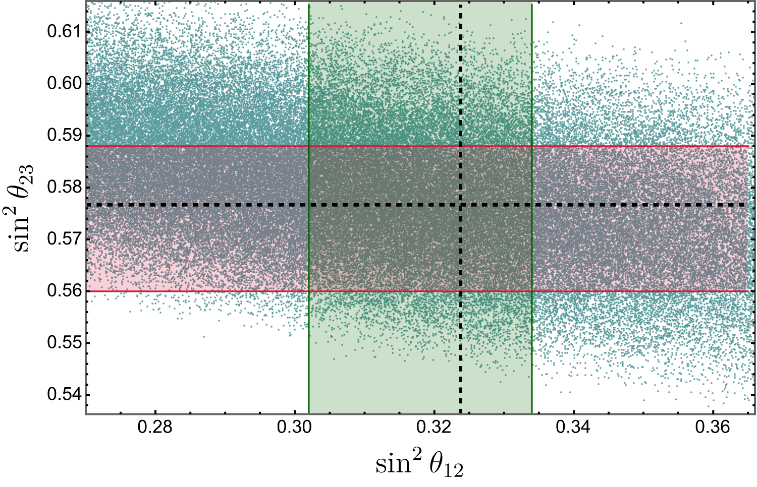
On the other hand, by varying our parameters around 30% of their best-fit point to generate data that are in the range of up to , we can obtain correlations between the leptonic CP violating phase and the atmospheric (see Fig. 1a) and reactor mixing angles (Fig. 1b). In addition, we can also see a correlation between the solar mixing angle with the reactor and atmospheric mixing angles (Fig. 1c and 1d, respectively), where our model obtains the following range of values for , , and , with all values of being in the experimental range of .
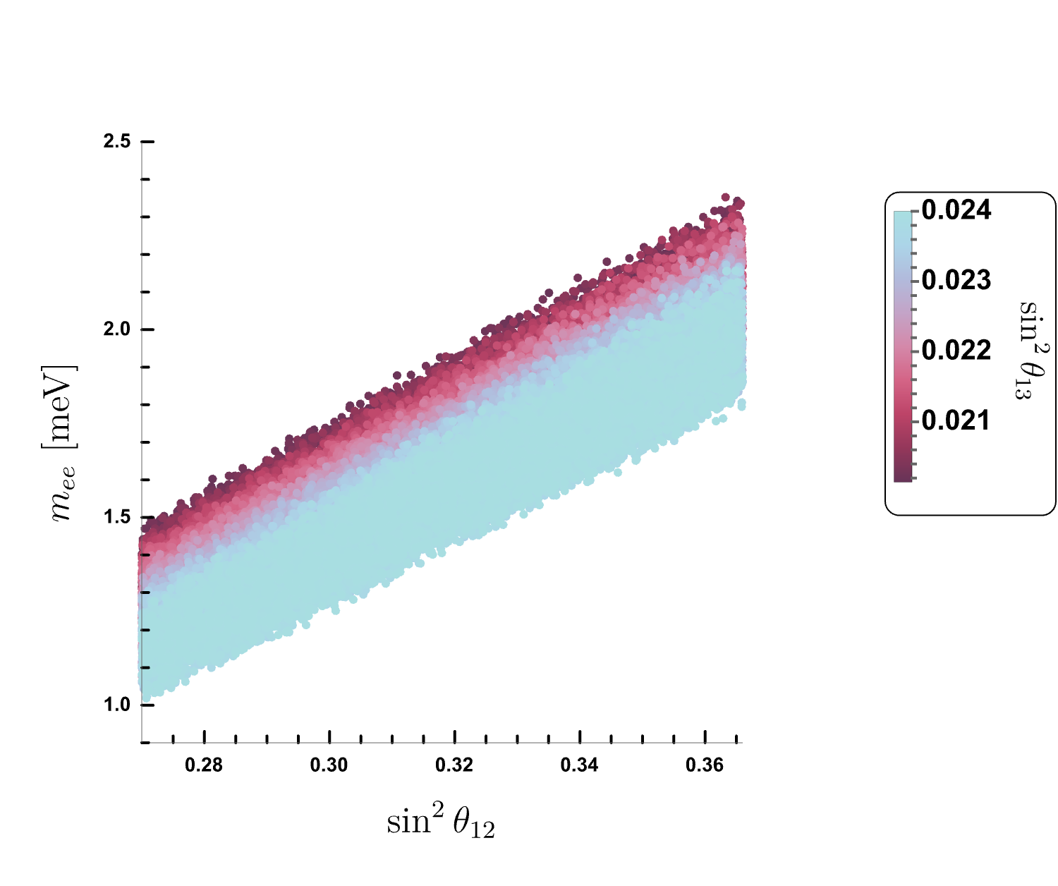
Furthermore, in our model we can obtain another observable, which corresponds to the effective Majorana neutrino mass parameter of the neutrinoless double beta decay without neutrinos. This observable provides information about the Majorana nature of neutrinos, where the shape of this mass parameter is given by:
| (18) |
where and are the matrix elements of the PMNS leptonic mixing matrix and the light active neutrino masses, respectively. The neutrinoless double beta () decay amplitude is proportional to . Fig. 2 shows the correlation between the Majorana neutrino effective mass parameter and the solar mixing parameter considering different values of the reactor mixing parameter . As can be seen in Fig. 2, the model predicts an effective mass parameter of the Majorana neutrino in the range . The current strictest experimental upper limit on the Majorana neutrino effective mass parameter, i.e., arises from the KamLAND-Zen boundary at decay half-life year [37].
IV Charged Lepton Flavor Violation
In the next section, we discuss the charged lepton flavor violation (cLFV) processes present due to the mixing between active and heavy sterile neutrinos. In this analysis, we focus in the one-loop decay where the branching ratios are given by [38, 39, 40]
| (19) | |||||
| (20) | |||||
where GeV is the total muon decay width, is the matrix that diagonalizes the light neutrinos mass matrix which, in our case, is equal to the PMNS matrix since the charged lepton mixing matrix is equal to the identity , as can be seen in Eq. (6). In addition, the matrix is given by
| (21) |
where and are the heavy Majorana mass and the Dirac neutrino submatrix, respectively.
The charged lepton flavor-violating processes and are highly suppressed in our model; however, for the process the model predicts values below the experimental limit, its value for our best-fit point being equal to,
| (22) |
Fig. 3 shows the correlation between the branching ratio and the mass of the heavy pseudo-Dirac neutrino . The green horizontal line and the shaded region in this plot represent the experimental limit given by MEG [41] collaboration,
| (23) |
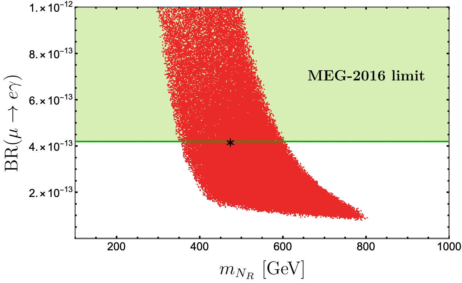
The red scatter points in Fig. 3 represent the random variation of the parameters around 30% of the best-fit point, while the black star corresponds to the value of the branching ratio given in Eq. (22). All red points are consistent with the neutrino oscillation experimental data at , and set the mass of the heavy pseudo-Dirac neutrino pair in the range , where the lowest bound of GeV arises from requiring a decay rate below its upper experimental limit.
V Conclusions
We have proposed a supersymmetric model based on the family symmetry, supplemented by auxiliary cyclic symmetries where the tiny neutrino masses are generated from a linear seesaw mechanism. In the proposed theory the Standard Model charged lepton mass hierarchy arises from the spontaneous breaking of the cyclic symmetries. The family symmetry yields a diagonal charged lepton mass matrix in the symmetry basis, where the leptonic mixings entirely arises from the neutrino sector. Our model provides a successful fit of the experimental values for the neutrino mass squared splittings, leptonic mixing angles and leptonic Dirac CP phase. We have analyzed its consequences on charged lepton flavor violation and found that the considered model predicts very small rates for the and decays but sizeable rates for the decay, within the reach of sensitivity of the forthcoming experiments, constraining the right-handed neutrino mass to be in a range.
Acknowledgments
A.E.C.H is supported by ANID-Chile FONDECYT 1210378, ANID PIA/APOYO AFB230003, ANID- Programa Milenio - code ICN2019_044, PIIC program of Universidad Técnica Federico Santa María and ANID Programa de Becas Doctorado Nacional code 21212041. IdMV acknowledges funding from Fundação para a Ciência e a Tecnologia (FCT) through the contract UID/FIS/00777/2020 and was supported in part by FCT through projects CFTP-FCT Unit 777 (UID/FIS/00777/2019), PTDC/FIS-PAR/29436/2017, CERN/FIS-PAR/0004/2019 and CERN/FIS-PAR/0008/2019 which are partially funded through POCTI (FEDER), COMPETE, QREN and EU. AECH thanks the Instituto Superior Técnico, Universidade de Lisboa for hospitality, where part of this work was done.
Appendix A The discrete group
The discrete group has the following 11 irreducible representations: one triplet , one antitriplet and nine singlets (), where and identify how the singlets transform under order 3 generators, corresponding to a and subgroups of .
| (24) |
Denoting and as the basis vectors for two -triplets , one finds:
| (26) |
where and .
References
- [1] G. C. Branco, J. M. Gerard, and W. Grimus, “GEOMETRICAL T VIOLATION,” Phys. Lett. B 136 (1984) 383–386.
- [2] I. de Medeiros Varzielas, S. F. King, and G. G. Ross, “Neutrino tri-bi-maximal mixing from a non-Abelian discrete family symmetry,” Phys. Lett. B 648 (2007) 201–206, arXiv:hep-ph/0607045.
- [3] E. Ma, “Neutrino Mass Matrix from Delta(27) Symmetry,” Mod. Phys. Lett. A 21 (2006) 1917–1921, arXiv:hep-ph/0607056.
- [4] E. Ma, “Near tribimaximal neutrino mixing with Delta(27) symmetry,” Phys. Lett. B 660 (2008) 505–507, arXiv:0709.0507 [hep-ph].
- [5] F. Bazzocchi and I. de Medeiros Varzielas, “Tri-bi-maximal mixing in viable family symmetry unified model with extended seesaw,” Phys. Rev. D 79 (2009) 093001, arXiv:0902.3250 [hep-ph].
- [6] I. de Medeiros Varzielas and D. Emmanuel-Costa, “Geometrical CP Violation,” Phys. Rev. D 84 (2011) 117901, arXiv:1106.5477 [hep-ph].
- [7] I. de Medeiros Varzielas, D. Emmanuel-Costa, and P. Leser, “Geometrical CP Violation from Non-Renormalisable Scalar Potentials,” Phys. Lett. B 716 (2012) 193–196, arXiv:1204.3633 [hep-ph].
- [8] G. Bhattacharyya, I. de Medeiros Varzielas, and P. Leser, “A common origin of fermion mixing and geometrical CP violation, and its test through Higgs physics at the LHC,” Phys. Rev. Lett. 109 (2012) 241603, arXiv:1210.0545 [hep-ph].
- [9] P. M. Ferreira, W. Grimus, L. Lavoura, and P. O. Ludl, “Maximal CP Violation in Lepton Mixing from a Model with Delta(27) flavour Symmetry,” JHEP 09 (2012) 128, arXiv:1206.7072 [hep-ph].
- [10] E. Ma, “Neutrino Mixing and Geometric CP Violation with Delta(27) Symmetry,” Phys. Lett. B 723 (2013) 161–163, arXiv:1304.1603 [hep-ph].
- [11] C. C. Nishi, “Generalized symmetries in flavor models,” Phys. Rev. D 88 no. 3, (2013) 033010, arXiv:1306.0877 [hep-ph].
- [12] I. de Medeiros Varzielas and D. Pidt, “Towards realistic models of quark masses with geometrical CP violation,” J. Phys. G 41 (2014) 025004, arXiv:1307.0711 [hep-ph].
- [13] A. Aranda, C. Bonilla, S. Morisi, E. Peinado, and J. W. F. Valle, “Dirac neutrinos from flavor symmetry,” Phys. Rev. D 89 no. 3, (2014) 033001, arXiv:1307.3553 [hep-ph].
- [14] I. de Medeiros Varzielas and D. Pidt, “Geometrical CP violation with a complete fermion sector,” JHEP 11 (2013) 206, arXiv:1307.6545 [hep-ph].
- [15] P. F. Harrison, R. Krishnan, and W. G. Scott, “Deviations from tribimaximal neutrino mixing using a model with symmetry,” Int. J. Mod. Phys. A 29 no. 18, (2014) 1450095, arXiv:1406.2025 [hep-ph].
- [16] E. Ma and A. Natale, “Scotogenic or Model of Neutrino Mass with Symmetry,” Phys. Lett. B 734 (2014) 403–405, arXiv:1403.6772 [hep-ph].
- [17] M. Abbas and S. Khalil, “Fermion masses and mixing in flavour model,” Phys. Rev. D 91 no. 5, (2015) 053003, arXiv:1406.6716 [hep-ph].
- [18] M. Abbas, S. Khalil, A. Rashed, and A. Sil, “Neutrino masses and deviation from tribimaximal mixing in (27) model with inverse seesaw mechanism,” Phys. Rev. D 93 no. 1, (2016) 013018, arXiv:1508.03727 [hep-ph].
- [19] I. de Medeiros Varzielas, “ family symmetry and neutrino mixing,” JHEP 08 (2015) 157, arXiv:1507.00338 [hep-ph].
- [20] F. Björkeroth, F. J. de Anda, I. de Medeiros Varzielas, and S. F. King, “Towards a complete SUSY GUT,” Phys. Rev. D 94 no. 1, (2016) 016006, arXiv:1512.00850 [hep-ph].
- [21] P. Chen, G.-J. Ding, A. D. Rojas, C. A. Vaquera-Araujo, and J. W. F. Valle, “Warped flavor symmetry predictions for neutrino physics,” JHEP 01 (2016) 007, arXiv:1509.06683 [hep-ph].
- [22] V. V. Vien, A. E. Cárcamo Hernández, and H. N. Long, “The flavor 3-3-1 model with neutral leptons,” Nucl. Phys. B 913 (2016) 792–814, arXiv:1601.03300 [hep-ph].
- [23] A. E. Cárcamo Hernández, H. N. Long, and V. V. Vien, “A 3-3-1 model with right-handed neutrinos based on the family symmetry,” Eur. Phys. J. C 76 no. 5, (2016) 242, arXiv:1601.05062 [hep-ph].
- [24] F. Björkeroth, F. J. de Anda, I. de Medeiros Varzielas, and S. F. King, “Leptogenesis in a SUSY GUT,” JHEP 01 (2017) 077, arXiv:1609.05837 [hep-ph].
- [25] A. E. Cárcamo Hernández, S. Kovalenko, J. W. F. Valle, and C. A. Vaquera-Araujo, “Predictive Pati-Salam theory of fermion masses and mixing,” JHEP 07 (2017) 118, arXiv:1705.06320 [hep-ph].
- [26] I. de Medeiros Varzielas, G. G. Ross, and J. Talbert, “A Unified Model of Quarks and Leptons with a Universal Texture Zero,” JHEP 03 (2018) 007, arXiv:1710.01741 [hep-ph].
- [27] N. Bernal, A. E. Cárcamo Hernández, I. de Medeiros Varzielas, and S. Kovalenko, “Fermion masses and mixings and dark matter constraints in a model with radiative seesaw mechanism,” JHEP 05 (2018) 053, arXiv:1712.02792 [hep-ph].
- [28] A. E. Cárcamo Hernández, H. N. Long, and V. V. Vien, “The first flavor 3-3-1 model with low scale seesaw mechanism,” Eur. Phys. J. C 78 no. 10, (2018) 804, arXiv:1803.01636 [hep-ph].
- [29] I. De Medeiros Varzielas, M. L. López-Ibáñez, A. Melis, and O. Vives, “Controlled flavor violation in the MSSM from a unified flavor symmetry,” JHEP 09 (2018) 047, arXiv:1807.00860 [hep-ph].
- [30] A. E. Cárcamo Hernández, S. Kovalenko, J. W. F. Valle, and C. A. Vaquera-Araujo, “Neutrino predictions from a left-right symmetric flavored extension of the standard model,” JHEP 02 (2019) 065, arXiv:1811.03018 [hep-ph].
- [31] A. E. Cárcamo Hernández, J. C. Gómez-Izquierdo, S. Kovalenko, and M. Mondragón, “ flavor singlet-triplet Higgs model for fermion masses and mixings,” Nucl. Phys. B 946 (2019) 114688, arXiv:1810.01764 [hep-ph].
- [32] E. Ma, “Scotogenic cobimaximal Dirac neutrino mixing from and ,” Eur. Phys. J. C 79 no. 11, (2019) 903, arXiv:1905.01535 [hep-ph].
- [33] F. Björkeroth, I. de Medeiros Varzielas, M. L. López-Ibáñez, A. Melis, and O. Vives, “Leptogenesis in with a Universal Texture Zero,” JHEP 09 (2019) 050, arXiv:1904.10545 [hep-ph].
- [34] A. E. Cárcamo Hernández and I. de Medeiros Varzielas, “ framework for cobimaximal neutrino mixing models,” Phys. Lett. B 806 (2020) 135491, arXiv:2003.01134 [hep-ph].
- [35] R. Gonzalez Felipe, H. Serodio, and J. P. Silva, “Neutrino masses and mixing in A4 models with three Higgs doublets,” Phys. Rev. D 88 no. 1, (2013) 015015, arXiv:1304.3468 [hep-ph].
- [36] P. F. de Salas, D. V. Forero, S. Gariazzo, P. Martínez-Miravé, O. Mena, C. A. Ternes, M. Tórtola, and J. W. F. Valle, “2020 global reassessment of the neutrino oscillation picture,” JHEP 02 (2021) 071, arXiv:2006.11237 [hep-ph].
- [37] KamLAND-Zen Collaboration, S. Abe et al., “First Search for the Majorana Nature of Neutrinos in the Inverted Mass Ordering Region with KamLAND-Zen,” arXiv:2203.02139 [hep-ex].
- [38] P. Langacker and D. London, “Lepton Number Violation and Massless Nonorthogonal Neutrinos,” Phys. Rev. D 38 (1988) 907.
- [39] L. Lavoura, “General formulae for f(1) — f(2) gamma,” Eur. Phys. J. C 29 (2003) 191–195, arXiv:hep-ph/0302221.
- [40] L. T. Hue, L. D. Ninh, T. T. Thuc, and N. T. T. Dat, “Exact one-loop results for in 3-3-1 models,” Eur. Phys. J. C 78 no. 2, (2018) 128, arXiv:1708.09723 [hep-ph].
- [41] MEG Collaboration, A. M. Baldini et al., “Search for the lepton flavour violating decay with the full dataset of the MEG experiment,” Eur. Phys. J. C 76 no. 8, (2016) 434, arXiv:1605.05081 [hep-ex].