First-principles Methodology for studying magnetotransport in magnetic materials

Abstract

Unusual magnetotransport behaviors such as temperature dependent negative magnetoresistance(MR) and bowtie-shaped MR have puzzled us for a long time. Although several mechanisms have been proposed to explain them, the absence of comprehensive quantitative calculations has made these explanations less convincing. In our work, we introduce a methodology to study the magnetotransport behaviors in magnetic materials. This approach integrates anomalous Hall conductivity induced by Berry curvature, with a multi-band ordinary conductivity tensor, employing a combination of first-principles calculations and semi-classical Boltzmann transport theory. Our method incorporates both the temperature dependency of relaxation time and anomalous Hall conductivity, as well as the field dependency of anomalous Hall conductivity. We initially test this approach on two-band models and then apply it to a Weyl semimetal css. The results, which align well with experimental observations in terms of magnetic field and temperature dependencies, demonstrate the efficacy of our approach. Additionally, we have investigated the distinct behaviors of magnetoresistance (MR) and Hall resistivities across various types of magnetic materials. This methodology provides a comprehensive and efficient means to understand the underlying mechanisms of the unusual behaviors observed in magneto-transport measurements in magnetic materials.

Large anomalous Hall effect (AHE) Shekhar et al. (2018); Wang et al. (2018); Li et al. (2020); Jiang et al. (2021a); Fujishiro et al. (2021); Chen et al. (2021); Ram et al. (2023) and unusual magnetotransport behaviors such as large magnetoresistance (MR) Ali et al. (2014); Shekhar et al. (2015); Kumar et al. (2017); Ram et al. (2023) or negative magnetoresistance (NMR) Yang et al. (2020); Ogasawara et al. (2021); Afzal et al. (2022); Zhu et al. (2023) are often observed in magnetic materials. Exploration of various MR and large AHE responses may lead to the novel electronic functionalities and efficient spintronic devices. Among them the most intriguing thing is the NMR. Several machanisms have been proposed in a lot of literature to explain the NMR, such as weak localization Bergmann (1984), electron magnon scattering Mihai et al. (2008); Raquet et al. (2002); Zhao et al. (2023a), etc. However, few researches study the impact the anomalous Hall effect brings to the MR especially the NMR quantitatively.

For quantitative analysis of the influence brought by AHE, calculations of ordinary conductivity and anomalous Hall conductivity (AHC) based on first-principles calculated tight-binding(TB) Hamiltonian is needed. Zhang et al have systematically studied the MR derived from ordinary conductivity tensor by using the Boltzmann transport theory in several realistic materials Zhang et al. (2019). The calculated MR curves show good agreement with available experimental data, within the momentum-independent approximation of relaxation time. Nevertheless, this approach has not been extended to the magnetic materials with non-negligible AHC, where numerous magnetotransport behaviors remain to be discussed.

The empirical relation for the Hall resistivity of magnetic materials are considered to be the summation of the ordinary part $\rho_{yx}^{O}$ and anomalous part $\rho_{yx}^{A}$, written as $\rho_{yx}=\rho_{yx}^{O}+\rho_{yx}^{A}$ Pugh (1930); Pugh and Lippert (1932). Conventionally $\rho_{yx}^{O}=R_{o}B_{z}$ and $\rho_{yx}^{A}=R_{s}M$, where $R_{o}$ is the ordinary Hall coefficient, $B_{z}$ is the perpendicular field and $R_{s}$ is the material dependent anomalous Hall coefficient. However this simple division of $\rho_{yx}$ may be invalid unless both the ordinary and anomalous Hall angles are small, as pointed by Zhao et al in Ref. Zhao et al. (2023b).

Conductivity, rather than resistivity, is more essential in describing the transport physics, considering that multiple carriers form parallel circuits contributing to the transport. Building on this perspective, our work develops a combined first-principles and semiclassical Boltzmann transport methodology to study magnetotransport in magnetic materials. We adopt the conductivity relation and extend it to multi-band magnetic materials as follows:

$${\bm{\sigma}}=\sum_{n}{\bm{\sigma}}_{n}^{O}(\bm{B},T)+\bm{\sigma}^{A}(\bm{B},T).$$ (1)

where $n$ is the index of $n$th band. ${\bm{\sigma}}_{n}^{O}(\bm{B},T)$ and $\bm{\sigma}^{A}(\bm{B},T)$ represent the ordinary conductivity of the $n$th band and the AHC respectively, both of which depend on temperature and magnetic field. These two conductivity tensors can be simulated through model settings or within a first-principles framework. In the main text, we focus on the formalism in the first-principles framework, and defer the discussions of model simulations in the Supplemental Materialsup .

By employing first-principles calculations and constructing tight-binding Hamiltonians with maximally localized Wannier functions Marzari and Vanderbilt (1997); Souza et al. (2001); Mostofi et al. (2008), we can calculate the ordinary conductivity and anomalous Hall conductivity. The number of target bands contributing to the conductivity near the Fermi surface is ensured by $k$-point sampling. By solving the Boltzmann equation with the approximation of momentum-independent relaxation time, we obtain the ordinary conductivity of the target bands Chambers (1952); Ashcroft and Mermin (1976); Zhang et al. (2019)

$$\begin{split}\bm{\sigma}_{n}^{O}(\bm{B},T)&=e^{2}\tau_{n}(T)\int_{\rm BZ}\frac{\mathop{}\!\mathrm{d}\bm{k}}{(2\pi)^{3}}(-\frac{\partial f(\epsilon,T)}{\partial\epsilon})_{\epsilon=\epsilon_{n}(\bm{k})}\\ &\times\bm{v}_{n}(\bm{k})\bar{\bm{v}}_{n}(\bm{k}),\end{split}$$ (2)

where $\tau_{n}(T)$ is the relaxation time of the $n$th band with temperature dependency , $f$ is the Fermi-Dirac distribution, $\bm{v}_{n}(\bm{k})$ and $\bar{\bm{v}}_{n}(\bm{k})$ is the velocity and weighted average velocity, respectively. By integrating the kinematic equation, we can determine the trajectory of $\bm{k}(t)$ and calculate $\bm{v}_{n}(\bm{k})$ and $\bar{\bm{v}}_{n}(\bm{k})$(Sec.S1 of the Supplemental Materialsup )

The intrinsic anomalous Hall conductivity can also be calculated by integrating the Berry curvature $\Omega_{n}^{\gamma}(\bm{k})$ in the Brillouin Zone Wang et al. (2006)

$$\begin{split}(\sigma_{\alpha\beta}^{A})_{s}&=-\varepsilon_{\alpha\beta\gamma}\frac{e^{2}}{\hbar}\sum_{n}\int_{\rm BZ}\frac{\mathop{}\!\mathrm{d}\bm{k}}{(2\pi)^{3}}f(\epsilon_{n}(\bm{k}))\Omega_{n}^{\gamma}(\bm{k})\end{split}$$ (3)

$(\sigma_{\alpha\beta}^{A})_{s}$ denotes the maximum intrinsic AHC when the magnetization that perpendicular to $\alpha$-$\beta$ plane is fully saturated. This magnetization may be spontaneously induced in ferromagnetic materials or be induced by an external field in paramagnetic and anti-ferromagnetic material. Although the AHC may exhibit a nonlinear dependence on magnetization, we adhere to the assumption that the AHC is proportional to the magnetization in magnets Zeng et al. (2006), and with the magnetization parallel to the magnetic field along $\hat{z}$ direction, one can write the AHC as

$$\sigma_{xy}^{A}(B,T)=\frac{M(B,T)}{M_{s}}(\sigma_{xy}^{A})_{s}.$$ (4)

where $M(B,T)$ and $M_{s}$ refer to the field and temperature-dependent magnetization and the saturated magnetization, respectively.

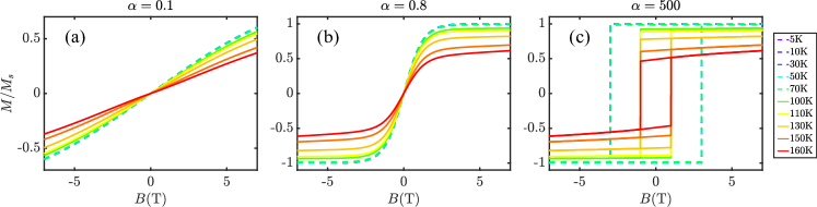
Figure 1: Temperature dependent magnetization curves, with dashed lines representing the magnetization at low temperatures and solid lines high temperatures. $\frac{M}{M_{s}}=\bar{S}\tanh{(\alpha B)}$ where $\alpha$ is a factor controlling the saturation speed. (a) $\alpha=0.1$. (b) $\alpha=0.8$. (c) $\alpha=500$ with coercive field $B_{c}=3\rm T$ at low temperatures and $B_{c}=1\rm T$ at high temperatures.

With the ordinary and anomalous parts of conductivity prepared, we employ Eq.(1) and invert it to calculate the resistivity $\bm{\rho}=\bm{\sigma}^{-1}$, and then MR and Hall resistivity analysis can be carried out. Notably, this approach is versatile, facilitating the calculation of a wide range of magnetic materials with various magnetization curve forms, leading to diverse MR and Hall resistivity curves. All the influences brought by different scattering mechanisms are considered in relaxation time $\tau_{n}(T)$.

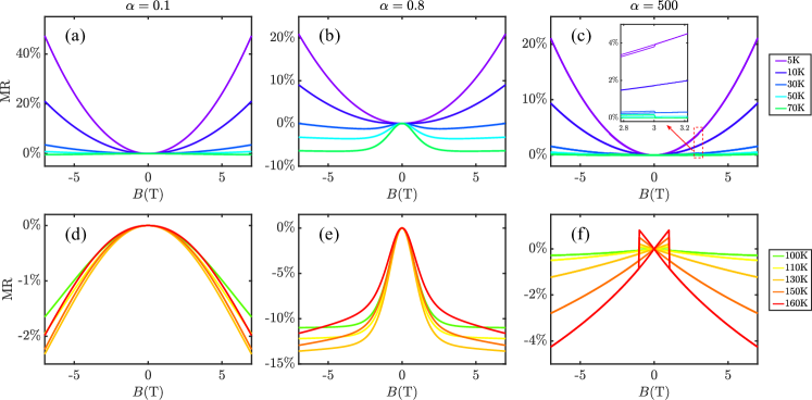
Figure 2: Field and temperature-dependent MR. (a), (d) $\alpha=0.1$, MR curves exhibit quadratic field dependence, showing positive values at low temperatures and negative values at high temperatures. (b), (e) $\alpha=0.8$, MR curves consist of two segments: initially dropping and then rising below 70 K, or continuously dropping with smaller slopes above 70 K. (c), (f) $\alpha=500$, MR curves are positive and quadratic below 70 K, with the inset highlighting behaviors at $B_{c}=3\rm T$. Above 70 K, MR curves turn negative and linear, displaying bowtie shapes.

To gain an intuitive understanding of our approach, we begin with understanding the magnetotransport of a two-band model, when taking into account the AHC $\sigma_{xy}^{A}$. The revised longitudinal and Hall resistivities can be obtained(Sec.S2 A of the Supplemental Materialsup )

$$\rho_{xx}=\frac{e\left[(n_{e}\mu_{e}\!+\!n_{h}\mu_{h})\!+\!(n_{e}\mu_{e}\mu_{h}^{2}\!+\!n_{h}\mu_{h}\mu_{e}^{2})B^{2}\right]}{e^{2}\left[(n_{e}\mu_{e}\!+\!n_{h}\mu_{h})^{2}+(n_{e}\!-\!n_{h})^{2}\mu_{e}^{2}\mu_{h}^{2}B^{2}\right]\!+\!D(B)},$$ (5)

$$\rho_{xy}=\frac{-e\left[(n_{h}\mu_{h}^{2}\!-\!\!n_{e}\mu_{e}^{2}\!)B\!+\!\mu_{e}^{2}\mu_{h}^{2}(n_{h}\!-\!n_{e})B^{3}\right]\!+\!C(B)}{e^{2}\left[(n_{e}\mu_{e}\!+\!n_{h}\mu_{h})^{2}\!+\!(n_{e}\!-\!n_{h})^{2}\mu_{e}^{2}\mu_{h}^{2}B^{2}\right]\!+\!D(B)}.$$ (6)

where $C(B)\!=\!(1\!+\!\mu_{e}^{2}B^{2})(1\!+\!\mu_{h}^{2}B^{2}){\sigma_{xy}^{A}}^{2}$ and $D(B)\!=\!2e\left[(\mu_{h}^{2}n_{h}\!-\!\mu_{e}^{2}n_{e})B\!+\!\mu_{e}^{2}\mu_{h}^{2}(n_{h}\!-\!n_{e})B^{3}\right]\sigma_{xy}^{A}\!+\!C(B)$ are the extra terms compared to the conventional two-band model whose MR is impossibly negative without $\sigma_{xy}^{A}$ included. In contrast, negative MR is attainable in our revised form of $\rho_{xx}$ in Eq.(5).

The key to achieving NMR lies in the competition between the increase in field-dependent terms in the numerator and denominator of $\rho_{xx}$. In the conventional two-band Drude’s model, the denominator always increases slower with the magnetic field than the numerator, resulting in positive MR. However, in our revised two-band model, the term $D(B)$ may contribute a significant additional increase with the field, leading to a greater growth in the denominator compared to the numerator, and thus facilitating NMR. To further illustrate it, note that in the denominator of $\rho_{xx}$, $\sigma_{xx}^{2}(0)$ appears as $e^{2}(n_{e}\mu_{e}+n_{h}\mu_{h})^{2}$, and by rewriting $D(B)$ as $2e\left[(\mu_{h}^{2}n_{h}\!-\!\mu_{e}^{2}n_{e})B\!+\!\mu_{e}^{2}\mu_{h}^{2}(n_{h}\!-\!n_{e})B^{3}\right]\tan\vartheta\sigma_{xx}(0)+(1\!+\!\mu_{e}^{2}B^{2})(1\!+\!\mu_{h}^{2}B^{2})\tan^{2}\vartheta\sigma^{2}_{xx}(0)$ where $\tan\vartheta=\sigma_{xy}^{A}/\sigma_{xx}(0)$ denotes the anomalous Hall angle(AHA), we can evaluate the contribution of $D(B)$ by the AHA. With sufficiently large AHA, NMR is attainable under the significant influence of $D(B)$. The emergence of NMR and the method to achieve large NMR are further analyzed in Sec.S2 C and Sec.S5 of the Supplemental Materialsup .

The temperature dependency of MR and Hall resistivities is attributed to the Fermi distribution, the temperature dependent magnetization $M(B,T)$ and mobility $\mu(T)$. For magnetization $M(B,T)$, we can directly adopt the curves of experiments, or alternatively generate them using specific formulas. Here we produce the magnetization curves using the following formula:

$$\frac{M(B,T)}{M_{s}}=\bar{S}\tanh{(\alpha B)},$$ (7)

where $\bar{S}$ is the average spin determined by mean field method with $qJ$ controlling the Curie temperature(Sec.S2 B of the Supplemental Materialsup ), and $\alpha$ is the factor controlling the saturating speed of magnetization.

Without lose of generality, we consider three forms of magnetization curves, corresponding to $\alpha=0.1$ and $\alpha=0.8$ without a coercive field, and $\alpha=500$ with a coercive field, to represent anti-ferrromagnetic or non-magnetic materials, soft magnets, and ferromagnets, respectively. Those curves, depicted in Fig.1, are derived from Eq.(7) with a Curie temperature of 175K. The dashed lines and solid lines represent the magnetization at low temperatures(5-70K) and high temperatures(100-160K) respectively. For $\alpha=0.1$, magnetization is nearly linear dependent on magnetic field, as depicted in Fig.1(a). For $\alpha=0.8$, magnetization grows linearly below the saturation field $B\approx 2$ T and is almost fully saturated above it, as depicted in Fig.1(b). For $\alpha=500$, magnetization is almost saturated instantaneously at first($B\approx 0$ T), as shown in Fig.S1(c)sup , similar to that of css in Fig.1(c) of Ref. Wang et al. (2018) or Fig.2(a) of Ref.Thakur et al. (2020). By extending the field-parallel magnetization curves to the anti-parallel configuration region up to the coercive field $B_{c}$, with an appropriate slope, we can obtain the hysteresis magnetization loops similar to that of css(Fig.1(d) of Ref.Guin et al. (2019)), as illustrated in Fig.1(c). For simplicity, we set $B_{c}=3$ T at low temperatures and $B_{c}=1$ T at high temperatures. The temperature and field dependent $\sigma_{xy}^{A}(B,T)$ is then attainable using Eq.(4) by setting a appropriate value for $(\sigma_{xy}^{A})_{s}$.

For the mobility $\mu(T)$, it is related to the relaxation time $\tau(T)$ by $\mu(T)=e\tau(T)/m$. We know that in the absence of magnetic field, according to the Drude model, $\tau(T)\propto 1/\rho(T)$ Chambers (2012), where $\rho(T)=\rho_{0}+f(T)$, $\rho_{0}$ is the residual resistivity and $f(T)$ comes from the temperature dependent scattering mechanisms such as electron-electron scattering and electron-phonon scattering et al. For simplicity we set $\rho(T)-\rho_{0}\propto T$. Certainly we can add some $T^{2},T^{5}$ scaling terms at low temperatures to make results more accurate, but it hardly affect the key features we care about in MR especially the NMR at high temperatures. Then the corresponding relaxation time has the formula of $\tau(T)=1/({\rm C}+{\rm A}T)$ and the formulas of mobility can be written as

$$\mu_{e}=\frac{e}{m_{e}}\frac{1}{{\rm C_{e}}+{\rm A_{e}}T},\quad\mu_{h}=\frac{e}{m_{h}}\frac{1}{{\rm C_{h}}+{\rm A_{h}}T}.$$ (8)

the parameters of Eq.(8) along with the carrier concentrations and the maximum anomalous Hall conductivity are set in Table S1sup .

With the above settings of the magnetization curve and relaxation time, the temperature and magnetic field dependent MR curves of our two-band model are shown in Fig.2. As comparison, the results of single-band model for all these magnetization forms are also shown and discussed in Sec.S4sup . For $\alpha=0.1$, the MR curves are quadratic, showing positive values at low temperatures and negative values at high temperatures, as depicted in Fig.2(a)(d). As discussed in Sec.S2 Csup , a linear field dependent AHA with a significant slope $\gamma$ (as shown in Fig.1(a)) is beneficial for achieving NMR. We found that the NMR reaches its maximum at 130K where AHA also reaches its maximum, indicating that strengthened AHA is responsible for the transition of MR from positive to negative. This MR behavior, transitioning from positive to negative, can also be observed in antiferromagnetic $\rm LaMn_{x}Sb_{2}$, where $\rm Mn$ occupancy $\rm x$ controls the strength of magnetization and thus AHA Slade et al. (2023).

For $\alpha=0.8$, MR curves consist of two segments. At low temperatures, they drop down first in the first segment (almost invisible at extremely low temperatures like 5K and 10K), then gradually rise in the second segment, as shown in Fig.2(b). At high temperatures, MR curves drop down rapidly in the first segment and slower in the second segment, as shown in Fig.2(e). The distinct MR behaviors in these segments stem from the growing patterns of magnetization. The first segment aligns with the rapidly increasing magnetization leading to a quick AHA rise and thus enhancing the negative slope of NMR. The second segment, corresponding to saturated magnetization, indicates a relatively stable AHA, lessening its impact on the negative slope of MR. This type of NMR is similar to that found in materials such as $\rm SrIrO_{3}$ Jaiswal et al. and $\rm Ni_{0.8}\rm Fe_{0.2}$ Jiang et al. (2021b), suggesting our proposed mechanism may underlie these observations.

For $\alpha=500$, the hysteresis magnetization loops appear rectangular-like at low temperatures and rhomboid-like at high temperatures, as depicted in Fig.1(c). At high temperatures, with slight positive slope $\gamma$ and large AHA in hysteresis loops, the MR curves exhibit negative and linear field dependency with bowtie shapes, as shown in Fig.2(f). At low temperatures, MR curves are quadratic and positive, and furthermore, jumps at the coercive field $B_{c}$ at 5 K but in contrast drops at $B_{c}$ at 30 K, as shown in Fig2(c). All these behaviors are in consistence with that of css Yang et al. (2020), and we meticulously discuss the origins underlying these unique behaviors in Sec.S2 Dsup .

Moving beyond model analysis, we employ first-principles calculations for css. Recognized as a magnetic Weyl semimetal with a stacked kagome lattice structure, css has attracted considerable attention for its large anomalous Hall angles (AHA) and particularly for its unusual magneto-transport behaviors, whose mechanisms remain not fully understood. In this study, we apply our first-principles methodology to explore these magnetotransport behaviors. The saturated AHC, calculated when magnetic moments are aligned with the magnetic field, is obtained using WannierToolsWu et al. (2018) with a Wannier tight-binding model constructed by Wannier90Pizzi et al. (2020) and VASPKresse and Furthmüller (1996). This is depicted in Fig.S3(b)sup , with a notable value of about 1205 S/cm at the Fermi level. This value closely approximates the findings in Ref.Wang et al. (2018) and the experimental value reported in Ref.Liu et al. (2018). Eq.(4) is employed and Eq.(7) with $\alpha=500$ and proper coercive field setting is used to produce the magnetization curves similar to the experimental curvesGuin et al. (2019). The temperature-dependent relaxation times are adapted by fitting to the experimental magnetoresistivity curves and Hall resistivity curves at different temperaturesZhang et al. (2019).

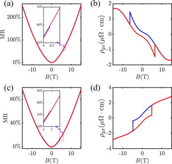
Figure 3: MR and Hall resistivity calculated for css from first-principles calculations. The insets of MR plots show the behaviors at $B_{c}$. (a), (b) MR and Hall resistivity at 2 K. (c), (d) MR and Hall resistivity at 30 K.

Fig.3 and Fig.4 present the MR and $\rho_{yx}$ curves at 2K, 30K, 150K, set with appropriate relaxation times. At 2K and 30K the MR curves are positive and quadratic field dependent. In contrast, at 150K, the MR curve becomes negative and linear field-dependent with a bowtie shape, consistent with experimental results. The plots of $\rho_{xx}$ and $\sigma_{xy}$ are available in Fig.S4sup . At 2 K, with $\tau_{h}=0.328\rm ps$ and $\tau_{e}=0.392\rm ps$, the MR is smaller in the magnetization configuration antiparallel to the field than in the parallel case, leading to a jump at the coercive field as shown in Fig.3(a). Conversely, at 30 K, with $\tau_{h}=0.208\rm ps$ and $\tau_{e}=0.192\rm ps$, the MR drops at the coercive field as show in Fig.3(c). These properties align with the experimental results Yang et al. (2020); Zeng et al. (2021) with no need for fine-tuning of the relaxation times. To explain these properties, we notice that at 2 K, $\tau_{h}<\tau_{e}$ but at 30 K, $\tau_{h}>\tau_{e}$, indicating that initially $\tau_{e}$ is larger but decreases faster than $\tau_{h}$. This leads to a sign change in $(\mu_{h}^{2}n_{h}-\mu_{e}^{2}n_{e})$ which is responsible for the MR transitioning from a jump to a drop at $B_{c}$, as detailed in Sec.S2 Dsup . Regarding the calculated Hall resistivity $\rho_{yx}$ in Fig.3(b)(d), the shapes of the hysteresis loops are also similar to those reported in Ref.Zhao et al. (2023b) in terms of trends. Additionally, we want to point out that the calculated MR at 2K is larger compared to the experimental value of Ref.Zhao et al. (2023b). This discrepancy is likely due to the absence of Berry curvature and orbital moment correction to the ordinary conductivity tensorXiao et al. (2005, 2010); Woo et al. (2022); Kokkinis et al. (2022), which may slow the reduction of $\sigma_{xx}^{O}$ and thus suppress the growing of MR.

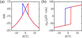
Figure 4: MR and Hall resistivity calculated for css from first-principles at 150 K. (a) MR. (b) Hall resistivity

At 150K, the relaxation time significantly decreases, resulting in a reduced value of the zero field longitudinal conductance. Consequently, this leads to an increase in the AHA. As mentioned in Sec.S2 Csup , a large and positive field dependent AHA helps to enlarge the negative MR. Fig.4 shows the plot of MR and Hall resistivity with $\tau_{h}=0.022\rm ps$ and $\tau_{e}=0.016\rm ps$. The negative MR achieves the value of -2.6% at $B=15$ T with AHA to be 0.24. Besides, the NMR curve exhibits significant linear characteristic. The $\rho_{yx}$ plot is also consistent with the supplementary information of Ref.Yang et al. (2020) both in shape and value. The consistency between the calculations and experiments for these unusual behaviors further confirm the validity of our approach.

In conclusion, we have developed a first-principles methodology to study magnetotransport in multi-band magnetic materials. This approach combines field and temperature-dependent ordinary conductivity and anomalous Hall conductivity. Initially applied to a two-band model, we successfully obtained revised longitudinal and Hall resistivities, showcasing a variety of MR and Hall curves with different magnetization forms. Subsequently, we applied this method to the realistic magnetic material css using first-principles calculations. The resulting unusual magnetotransport behaviors are consistent with experimental results, indicating the validity of our calculations. Our methodology may serve as a potent tool to study the magnetotransport properties across a wide range of magnetic materials. For further research, consideration could be given to the field dependency of residual resistivity $\rho_{0}$ due to spin disorder scatterings Haas (1968) or corrections to the ordinary conductivity induced by Berry curvature and orbital moment.

This work was supported by the National Key Research and Development Program of China (Grant No. 2023YFA1607400, 2022YFA1403800), the National Natural Science Foundation of China (Grant No.12274436, 11925408, 11921004), the Science Center of the National Natural Science Foundation of China (Grant No. 12188101), and H.W. acknowledge support from the Informatization Plan of the Chinese Academy of Sciences (CASWX2021SF-0102).

References

- Shekhar et al. (2018) C. Shekhar, N. Kumar, V. Grinenko, S. Singh, R. Sarkar, H. Luetkens, S.-C. Wu, Y. Zhang, A. C. Komarek, E. Kampert, et al., Proceedings of the National Academy of Sciences 115, 9140 (2018).
- Wang et al. (2018) Q. Wang, Y. Xu, R. Lou, Z. Liu, M. Li, Y. Huang, D. Shen, H. Weng, S. Wang, and H. Lei, Nature communications 9, 3681 (2018).
- Li et al. (2020) P. Li, J. Koo, W. Ning, J. Li, L. Miao, L. Min, Y. Zhu, Y. Wang, N. Alem, C.-X. Liu, et al., Nature communications 11, 3476 (2020).
- Jiang et al. (2021a) W. Jiang, D. J. P. de Sousa, J.-P. Wang, and T. Low, Phys. Rev. Lett. 126, 106601 (2021a).
- Fujishiro et al. (2021) Y. Fujishiro, N. Kanazawa, R. Kurihara, H. Ishizuka, T. Hori, F. S. Yasin, X. Yu, A. Tsukazaki, M. Ichikawa, M. Kawasaki, et al., Nature communications 12, 317 (2021).
- Chen et al. (2021) D. Chen, C. Le, C. Fu, H. Lin, W. Schnelle, Y. Sun, and C. Felser, Phys. Rev. B 103, 144410 (2021).
- Ram et al. (2023) D. Ram, J. Singh, M. K. Hooda, K. Singh, V. Kanchana, D. Kaczorowski, and Z. Hossain, Phys. Rev. B 108, 235107 (2023).
- Ali et al. (2014) M. N. Ali, J. Xiong, S. Flynn, J. Tao, Q. D. Gibson, L. M. Schoop, T. Liang, N. Haldolaarachchige, M. Hirschberger, N. P. Ong, et al., Nature 514, 205 (2014).
- Shekhar et al. (2015) C. Shekhar, A. K. Nayak, Y. Sun, M. Schmidt, M. Nicklas, I. Leermakers, U. Zeitler, Y. Skourski, J. Wosnitza, Z. Liu, et al., Nature Physics 11, 645 (2015).
- Kumar et al. (2017) N. Kumar, Y. Sun, N. Xu, K. Manna, M. Yao, V. Süss, I. Leermakers, O. Young, T. Förster, M. Schmidt, et al., Nature Communications 8, 1642 (2017).
- Yang et al. (2020) S.-Y. Yang, J. Noky, J. Gayles, F. K. Dejene, Y. Sun, M. Dörr, Y. Skourski, C. Felser, M. N. Ali, E. Liu, and S. S. P. Parkin, Nano Letters 20, 7860 (2020).
- Ogasawara et al. (2021) T. Ogasawara, K.-K. Huynh, T. Tahara, T. Kida, M. Hagiwara, D. Arčon, M. Kimata, S. Y. Matsushita, K. Nagata, and K. Tanigaki, Phys. Rev. B 103, 125108 (2021).
- Afzal et al. (2022) W. Afzal, Z. Yue, Z. Li, M. Fuhrer, and X. Wang, Journal of Physics and Chemistry of Solids 161, 110489 (2022).
- Zhu et al. (2023) Y. Zhu, C.-Y. Huang, Y. Wang, D. Graf, H. Lin, S. H. Lee, J. Singleton, L. Min, J. C. Palmstrom, A. Bansil, et al., Communications Physics 6, 346 (2023).
- Bergmann (1984) G. Bergmann, Physics Reports 107, 1 (1984).
- Mihai et al. (2008) A. Mihai, J. Attané, A. Marty, P. Warin, and Y. Samson, Physical Review B 77, 060401 (2008).
- Raquet et al. (2002) B. Raquet, M. Viret, E. Sondergard, O. Cespedes, and R. Mamy, Physical Review B 66, 024433 (2002).
- Zhao et al. (2023a) J. Zhao, B. Jiang, S. Zhang, L. Wang, E. Liu, Z. Li, and X. Wu, Physical Review B 107, 085203 (2023a).
- Zhang et al. (2019) S. Zhang, Q. Wu, Y. Liu, and O. V. Yazyev, Physical Review B 99, 035142 (2019).
- Pugh (1930) E. M. Pugh, Phys. Rev. 36, 1503 (1930).
- Pugh and Lippert (1932) E. M. Pugh and T. W. Lippert, Phys. Rev. 42, 709 (1932).
- Zhao et al. (2023b) J. Zhao, B. Jiang, J. Yang, L. Wang, H. Shi, G. Tian, Z. Li, E. Liu, and X. Wu, Physical Review B 107, L060408 (2023b).
- (23) See Supplemental Material at URL_will_be_inserted_by_publisher for details of the Boltzmann transport theory, model simulations and analysis, additional information for the two-band model and semimetal, meticulous analysis for the single-band model, and approach to obtain large negative MR.
- Marzari and Vanderbilt (1997) N. Marzari and D. Vanderbilt, Physical review B 56, 12847 (1997).
- Souza et al. (2001) I. Souza, N. Marzari, and D. Vanderbilt, Physical Review B 65, 035109 (2001).
- Mostofi et al. (2008) A. A. Mostofi, J. R. Yates, Y.-S. Lee, I. Souza, D. Vanderbilt, and N. Marzari, Computer physics communications 178, 685 (2008).
- Chambers (1952) R. G. Chambers, Proceedings of the Physical Society. Section A 65, 458 (1952).
- Ashcroft and Mermin (1976) N. Ashcroft and N. Mermin, Solid State Physics, HRW international editions (Holt, Rinehart and Winston, 1976).
- Wang et al. (2006) X. Wang, J. R. Yates, I. Souza, and D. Vanderbilt, Phys. Rev. B 74, 195118 (2006).
- Zeng et al. (2006) C. Zeng, Y. Yao, Q. Niu, and H. H. Weitering, Physical review letters 96, 037204 (2006).
- Thakur et al. (2020) G. S. Thakur, P. Vir, S. N. Guin, C. Shekhar, R. Weihrich, Y. Sun, N. Kumar, and C. Felser, Chemistry of Materials 32, 1612 (2020).
- Guin et al. (2019) S. N. Guin, P. Vir, Y. Zhang, N. Kumar, S. J. Watzman, C. Fu, E. Liu, K. Manna, W. Schnelle, J. Gooth, et al., Advanced Materials 31, 1806622 (2019).
- Chambers (2012) R. G. Chambers, Electrons in metals and semiconductors (Springer Science & Business Media, 2012).
- Slade et al. (2023) T. J. Slade, A. Sapkota, J. M. Wilde, Q. Zhang, L.-L. Wang, S. H. Lapidus, J. Schmidt, T. Heitmann, S. L. Bud’ko, and P. C. Canfield, Phys. Rev. Mater. 7, 114203 (2023).
- (35) A. K. Jaiswal, R. Eder, D. Wang, V. Wollersen, M. L. Tacon, and D. Fuchs, arXiv:2307.06064 .
- Jiang et al. (2021b) N. Jiang, B. Yang, Y. Bai, Y. Jiang, and S. Zhao, Nanoscale 13, 11817 (2021b).
- Wu et al. (2018) Q. Wu, S. Zhang, H.-F. Song, M. Troyer, and A. A. Soluyanov, Computer Physics Communications 224, 405 (2018).
- Pizzi et al. (2020) G. Pizzi, V. Vitale, R. Arita, S. Blügel, F. Freimuth, G. Géranton, M. Gibertini, D. Gresch, C. Johnson, T. Koretsune, J. Ibañez-Azpiroz, H. Lee, J.-M. Lihm, D. Marchand, A. Marrazzo, Y. Mokrousov, J. I. Mustafa, Y. Nohara, Y. Nomura, L. Paulatto, S. Poncé, T. Ponweiser, J. Qiao, F. Thöle, S. S. Tsirkin, M. Wierzbowska, N. Marzari, D. Vanderbilt, I. Souza, A. A. Mostofi, and J. R. Yates, Journal of Physics: Condensed Matter 32, 165902 (2020).
- Kresse and Furthmüller (1996) G. Kresse and J. Furthmüller, Phys. Rev. B 54, 11169 (1996).
- Liu et al. (2018) E. Liu, Y. Sun, N. Kumar, L. Muechler, A. Sun, L. Jiao, S.-Y. Yang, D. Liu, A. Liang, Q. Xu, et al., Nature physics 14, 1125 (2018).
- Zeng et al. (2021) Q. Zeng, G. Gu, G. Shi, J. Shen, B. Ding, S. Zhang, X. Xi, C. Felser, Y. Li, and E. Liu, Science China Physics, Mechanics & Astronomy 64, 287512 (2021).
- Xiao et al. (2005) D. Xiao, J. Shi, and Q. Niu, Phys. Rev. Lett. 95, 137204 (2005).
- Xiao et al. (2010) D. Xiao, M.-C. Chang, and Q. Niu, Rev. Mod. Phys. 82, 1959 (2010).
- Woo et al. (2022) S. Woo, B. Min, and H. Min, Phys. Rev. B 105, 205126 (2022).
- Kokkinis et al. (2022) E. K. Kokkinis, G. Goldstein, D. V. Efremov, and J. J. Betouras, Phys. Rev. B 105, 155123 (2022).
- Haas (1968) C. Haas, Phys. Rev. 168, 531 (1968).