Maximum entropy in dynamic complex networks

Abstract

Understanding common properties of different systems is a challenging task for interdisciplinary research. By representing these systems as complex networks, different fields facilitate their comparison. Common properties can then be extracted by network randomisation, in which a stochastic process preserves some properties of the network modifying others. If different systems exhibit statistically similar characteristics after being randomised by the same process, then these characteristics are taken to be explained by the preserved properties. The method of maximum entropy provides a way to completely bypass the construction of specific randomisation processes, directly obtaining ensembles of fully randomised networks,knowing that these contain no information beyond the imposed properties. The perspective of randomisation processes with associated dynamics has been used to obtain important and widespread properties of networks, suggesting that these are better explained from a dynamic perspective. In this work we use the maximum entropy based principle of maximum caliber to construct the evolution of an ensemble of networks based on constraints representing properties with known values throughout the evolution. We focus on the particular cases of dynamics resulting from conserved and variable number of links, comparing each to simulations of randomisation processes that obey the same constraints. We find that the simulations produce the same ensemble evolution as maximum caliber, that the equilibrium distributions converge to known stationary results of maximum entropy given the same constraints, discuss connections to other maximum entropy approaches to network dynamics, and conclude by pointing out several avenues of future research.

I Introduction

Complex networks is a growing field of science that studies interacting systems, from molecular [1, 2] to socio-economic scales [3, 4]. The ability to describe such a wide range of phenomena stems from the fact that networks focus on the topology of the interactions, meaning which components affect which, instead of specifics such as the origin of the interactions or their effect on the components. This is achieved through an adjacency matrix, a matrix $W$ in which each row $i$ and each column $j$ represent a specific node (component) of the network, and the value $w_{ij}$ at the location given by the row and column describe the state of the interaction from the node $i$ to $j$ [5]. A typical example is that when interactions are described by only on/off states, $w_{ij}$ is a binary variable with $1$ representing active connections and $0$ inactive ones. In this case the network is classified as binary . Moreover, if links are reciprocal (if $i$ affects $j$ then $j$ affects $i$), the adjacency matrix is symmetric $w_{ij}=w_{ji}$ and the network is classified as undirected . Whichever the type of network is chosen to represent the system of interest, the fact remains that network properties (i.e. calculated on the network representation as opposed to on the system itself) can be used to compare entirely different systems and identify common behaviours.

In the search for (network) properties that explain these common behaviours, network randomisation [8, 9, 10] is a recurrently used tool. A common way to randomise a network is to produce changes in it by repetition of a randomisation step (for example, connecting and disconnecting nodes) in such a way that hypothesised explanatory properties of common behaviours are unaffected (for example, conserving the total number of connections in the whole network or of each node). The successive repetition of the randomisation step then gradually removes information beyond the imposed properties, and multiple realisations of the process produces samples of randomised networks. If the behaviour we wish to explain is observed in the randomised networks then it can be attributed to the hypothesised explaining property.

The method of maximum entropy is another approach to randomisation [11, 12, 13, 14]. Its advantage is that it completely skips the construction of randomisation steps that progressively remove information on non-explaining properties. Instead, the distribution that maximises Shannon entropy subject to explaining properties as constraints is guaranteed to correspond to the ensemble of networks that are maximally unbiased with respect to non-explaining properties . This allows for samples to be drawn from the distribution and for the calculation of properties of the ensemble distribution as functions of the imposed properties.

However, randomisation as a process has provided significant insight on structural properties of real systems [16, 17]. This is understood to be due to the fact that real networks exist in a balance between order (no randomisation) and disorder (full randomisation, with only the explaining properties preserved), with different systems on different ranges of the scale. Where this balance lies is the result of dynamical processes such as link creation, relocation and destruction specific to the system, so a randomisation process in steps allows one to capture this dynamics and therefore describe out-of-equilibrium processes statistically. Maximum caliber [18, 19, 20, 21, 22] provides a robust entropy-based framework for non-stationary processes, as a dynamic counterpart for traditional entropy maximisation and an unbiased alternative to randomisation steps. Our goal is to use this principle, along with constraints corresponding properties of specific randomisation processes, to remove the need for an arbitrarily defined step and multiple repetition of it to estimate the ensemble evolution, instead describing it directly through the dynamics of the ensemble distribution.

Maximum caliber proposes, in rather general terms, that for non-stationary probability distributions each path $\Gamma=(x_{t})_{t=0}^{T}$ that a variable $x_{t}$ can take over time defines a random variable $\Gamma$ with Shannon entropy $S=-\sum_{\Gamma}p(\Gamma)\ln(p(\Gamma))$. Constraints on the average value of a path can then be written as $\sum_{\Gamma}p(\Gamma)f_{n}(\Gamma)=a_{n}$, yielding path distributions $p(\Gamma)=\exp(-\sum_{n}\lambda_{n}f_{n}(\Gamma))$ by maximisation of the Lagrangian $\mathcal{L}=S+\sum_{n}\lambda_{n}(a_{n}-\sum_{\Gamma}p(\Gamma)f_{n}(\Gamma))$. This is a remarkably general result, based only on realising that just as equilibrium states $x$ are random variables, so are the full trajectories $\Gamma$. Note that there is no restriction on $f_{n}$ (for example, it can be time-dependent taking into account the history of a variable) beyond that the imposed constraint values are well defined (for example, if $f_{n}$ represents a second moment, its value $a_{n}$ cannot be negative). However, it is not always clear what transitions (i.e. how to update states) define these trajectories from the dynamical point of view. It has been pointed out that Markov processes emerge in this context when constraints are defined on individual instants [19, 23], but in this regard, the approach of entropic dynamics provides more intuition [24, 25, 26]. It produces results on the transition matrix $p(x_{t+1}|x_{t})$ by minimizing the Kullback-Liebler divergence $\sum_{x_{t+1},x_{t}}p(x_{t+1}|x_{t})\ln(p(x_{t+1}|x_{t}))/q(x_{t+1}|x_{t}))$, which is a generalised form of minus the Shannon entropy reducing to it when $q(x_{t+1}|x_{t})$ (the prior distribution) is uniform [27]. The latter method is less well established due to the entropy functional being defined on distributions of random variables, while entropic dynamics applies the same functional to conditional distributions. Yet, to the best of our knowledge a connection between these approaches (and in particular, to maximum caliber) has not been made.

In this work we show how to construct the evolution of a network ensemble randomisation process conserving the number of links based on the principle of maximum caliber. This approach places emphasis on the fact that, because maximum caliber is able to predict distributions on the full trajectory of a random variable over time, it should be able to update a trajectory distribution which is interpreted as the history of the process. We show through simulations that the resulting evolutions are equivalent to multiple realisations of Watts-Strogatz rewiring (a well-known randomisation process that conserves the number of links in the network [16]), converging to an Erdös-Rényi random graph model (the equilibrium maximum entropy ensemble obtained by specifying the number of links in the network). Next, we modify the constraints in order to allow for controlled variation over time of the average number of links. Comparing to simulations of a rewiring process where links are also added or removed at certain rates, we show that maximum caliber also reproduces the behaviour of the modified process. In both cases the state of the network distribution at long times matches an Erdös-Rényi ensemble (the known stationary maximum entropy result) with the number of links defining the evolution being, in general, time dependent. In appendix A we pay attention to the difference between Markov and non-Markov processes in this context, finding it to be determined by the constraints used instead of an imposed property of the dynamical model. In appendix B we study the particular case of degree preserving rewiring, comparing simulations to the resulting ensemble dynamics for constraints different from the total number of links of the network. We then discuss the relation of our results to entropic dynamics and maximum entropy production in the information theoretic perspective, and conclude by discussing some of the possibilities for future work that this method offers.

II Methods and simulations

II.1 Maximum entropy Watts Strogatz rewiring

A single Watts-Strogatz rewiring step of choosing, uniformly and at random, one among $L$ links of a binary undirected network and placing it among the $N(N-1)/2-L$ disconnected pairs of nodes, also uniformly at random . This may be intuitively regarded as a dynamic extension of the Erdös-Rényi model for two reasons. First, it obeys the constraint of fixing the number of links, which results in the Erdös-Rényi network distribution in a maximum entropy setting. Second, the asymptotic state of the distribution (after many realisations of the rewiring) is an Erdös-Rényi distribution, meaning that an Erdos-Renyi ensemble can be considered as the equilibrium state of the process. Our goal here is to show that this idea is more than heuristic by constructing the randomisation process from the same constraints. Given the constraint of conservation of number of links, we will show that maximum caliber can produce a markovian process which is statistically identical to Watts-Strogatz rewring.

First, recall that in equilibrium entropy maximisation, links are considered independent a-priori. With the same assumption the entropy of a binary undirected network with a sequence of connection values $\vec{X}_{T}=(x_{o},x_{1},x_{2},...,x_{T})$ between the pair $i,j$ given a probability $p_{ij}(\vec{X}_{T})$ is

$$S=-\sum_{i,j>i}\sum_{\vec{X}_{T}}p_{ij}(\vec{X}_{T})\ln(p_{ij}(\vec{X}_{T}))\,.$$ (1)

As constraints, first consider that the average number of links at a time $t$ in the evolution of the network can be written as $L_{t}=\sum_{x_{t}}x_{t}p_{ij}(x_{t})=\sum_{\vec{X}_{T}}x_{t}p_{ij}(\vec{X}_{T})$. The conservation of the average number of links between two successive time steps is then simply

$$\sum_{i,j>i}\sum_{\vec{X}_{T}}(x_{T}-x_{T-1})p_{ij}(\vec{X}_{T})=0\,.$$ (2)

In this perspective, the constraint is derived from the sequence of values that the average number of links takes at each time in the evolution, essentially $\vec{L}_{T}=(L_{o},L_{1},L_{2},...,L_{T})$. This implies that the resulting trajectories are Markov as each value $L_{t}$ depends only on the state of the network at time $t$ [19]. However, in appendix A we show an alternative way to derive this constraint which does not build on values that depend only on states at given times. We also consider cases of other constraints which imply that obtaining Markovian processes in this context depends on the choice of constraints.

Next, we include the constraint of marginalisation

$$\sum_{x_{T}}p_{ij}(\vec{X}_{T})=p_{ij}(\vec{X}_{T-1})$$ (3)

which imposes the history of the network by providing the (distribution of) trajectories of link connection values $\vec{X}_{T-1}$ for each pair of nodes $i,j$. Note that it also replaces the normalisation of the full trajectory, implying instead that the measure of the (initial) distribution must be conserved. In this form, the state $x_{T-1}$ (which will be updated according to the process that corresponds to choosing any particular set of constraints) can be constructed through any method, matching or not the process at the following step. For example, in one experiment a network may be set up in a very specific state by a very complicated method, while in another experiment the same state may be obtained in a simpler way. How that state will evolve from there on, and whether it is dependent or not on how the state was set up depends on the specific process, defined by the constraints imposed. Once we obtain the updated trajectory, it becomes the history for the following state, independently of whether the history is constructed by a single process or in stages of different ones. In particular, we will see that the constraints we choose here produce a Markov process, meaning that the only relevant information is $x_{T-1}$, the last state in the history.

Finally, one more constraint is required. In Watts-Strogatz rewiring, the process is defined by replacing one link at a time . This means that the Hamming distance between two successive states of the adjacency matrix of a network undergoing a rewiring process  will have a value of $2$ (as in one position the link is removed and in another it is placed, changing values in both). This can be written as

$$\sum_{i,j>i}\sum_{\vec{X}_{T}}|x_{T}-x_{T-1}|p_{ij}(\vec{X}_{T})=2\,,$$ (4)

defining the time scale of the dynamics .

The Lagrangian is therefore

$$\mathcal{L}=S +\sum_{ij,\vec{X}_{T-1}}\lambda_{ij\vec{X}_{T-1}}\left(p_{ij}(\vec{X}_{T-1})-\sum_{x_{T}}p_{ij}(\vec{X}_{T})\right)$$ (5)

$$+\lambda_{a}\left(0-\sum_{ij>i}\sum_{\vec{X}_{T}}(x_{T}-x_{T-1})p_{ij}(\vec{X}_{T})\right)$$

$$+\lambda_{b}\left(2-\sum_{ij>i}\sum_{\vec{X}_{T}}|x_{T}-x_{T-1}|p_{ij}(\vec{X}_{T})\right)\,,$$

maximised by

$$\frac{\partial\mathcal{L}}{\partial p_{kl}(\vec{Y}_{T}=(y_{T},\vec{Y}_{T-1}))}=0$$ (6)

$$\Rightarrow p_{kl}(y_{T},\vec{Y}_{T-1})=$$

$$=\exp{\left(-\left[1+\lambda_{kl\vec{Y}_{T-1}}\right]\right)}\times$$

$$~{}~{}~{}~{}\exp{\left(-\left[\lambda_{a}(y_{T}-y_{T-1})+\lambda_{b}|y_{T}-y_{T-1}|\right]\right)}\,.$$

Marginalisation requires that

$$\exp\left(-1-\lambda_{kl\vec{Y}_{T-1}}\right)=$$ (7)

$$=\frac{p_{kl}(\vec{Y}_{T-1})}{\sum_{y_{T}}\exp(-\lambda_{a}(y_{T}-y_{T-1})-\lambda_{b}|y_{T}-y_{T-1}|))}$$

which, when introduced into eq. 6, becomes

$$p_{kl}(y_{T},\vec{Y}_{T-1})=$$ (8)

$$=\frac{\exp(-\lambda_{a}(y_{T}-y_{T-1})-\lambda_{b}|y_{T}-y_{T-1}|))}{\sum_{x_{T}}\exp(-\lambda_{a}(x_{T}-y_{T-1})-\lambda_{b}|x_{T}-y_{T-1}|)}p_{kl}(\vec{Y}_{T-1})$$

$$\Rightarrow p_{kl}(y_{T}|\vec{Y}_{T-1})=$$

$$=\frac{\exp(-\lambda_{a}(y_{T}-y_{T-1})-\lambda_{b}|y_{T}-y_{T-1}|))}{\sum_{x_{T}}\exp(-\lambda_{a}(x_{T}-y_{T-1})-\lambda_{b}|x_{T}-y_{T-1}|)}\,.$$

This is, by definition, a Markov process (it depends only on the updated and previous states $y_{T}$ and $y_{T-1}$) as a clear consequence of constraints referencing the previous state of the distribution only. Note that, independently of the parameters that $\lambda_{a}$ and $\lambda_{b}$ take to impose the constraints, the transition matrix is independent of the pair of nodes it connects. As the states are binary, the transition matrix defines link annihilation and creation probabilities $a$ (annihilation, $y_{T-1}=1\rightarrow y_{T}=0$ ) and $c$ (creation, $y_{T-1}=0\rightarrow y_{T}=1$) respectively,

$$p_{kl}(y_{T} |y_{T-1})=\begin{pmatrix}1-c&a\\ c&1-a\end{pmatrix}$$ (9)

$$=\begin{pmatrix}\frac{1}{1+\exp(-(\lambda_{a}+\lambda_{b}))}&\frac{1}{1+\exp(\lambda_{a}-\lambda_{b})}\\ \frac{1}{1+\exp(\lambda_{a}+\lambda_{b})}&\frac{1}{1+\exp(-(\lambda_{a}-\lambda_{b}))}\end{pmatrix}$$

where the entries with values $1-c$ and $1-a$ result from the marginalisation constraint and the dependence of these probabilities on $\lambda_{a}$ and $\lambda_{b}$.

Finally, noting that the two remaining constraints can be written simply as sums over the state at times $T$ and $T-1$,

$$0 =\sum_{i,j>i}p_{ij}(1,0)-p_{ij}(0,1)$$ (10)

$$=\sum_{i,j>i}cp_{ij}(0)-ap_{ij}(1)$$

$$=(N(N-1)/2-L)c-aL$$

and

$$2 =\sum_{i,j>i}p_{ij}(1,0)+p_{ij}(0,1)$$ (11)

$$=(N(N-1)/2-L)c+aL$$

$$\therefore~{}~{}~{}~{}c=\frac{1}{N(N-1)/2-L}~{}~{}~{}~{}~{}~{}~{}~{}a=\frac{1}{L}$$ (12)

defining the transition matrix and with it a single step in the randomisation process, that updates the probability of link states according to

$$p_{ij}(x_{T})=\sum_{x_{T-1}}p_{ij}(x_{T}|x_{T-1})p_{ij}(x_{T-1})\,.$$ (13)

With this result, we can update the probability of a link existing (or not) at time $T$ given its probability of existing (or not) at the previous time $T-1$.

Because of how the constraints were chosen, the evolution of the network ensemble distribution (i.e. $p_{ij}(\vec{X}_{T})$) as updated by the creation and annihilation probabilities is expected to match the distribution of trajectories over realisations of $T$ steps of Watts-Strogatz rewiring. Typically all these realisations start from single network defined by its adjacency matrix $X$, and different realisations show how the evolution may vary within a certain number of steps. In the maximum entropy perspective, this is acheived by setting $p_{ij}(x_{o})=1$ if $x_{o}=X_{ij}$ and $p_{ij}(x_{o})=0$ otherwise (as any sample from this distribution will match $X_{ij}$). However, the fact that the maximum entropy perspective can start from any $p_{ij}(x_{o})$ suggests that realisations can also draw (different) initial networks $X$ from an ensemble defined by an initial distribution $p_{ij}(x_{o})$. In both cases, the estimation of trajectory distribution evolution is achieved by counting, over realisations, how often nodes $i$ and $j$ are connected (or not) at a specific time $t$. This should match $p_{ij}(x_{t}=1)$ (or $p_{ij}(x_{t}=0)$) according to $t$ updates of $p_{ij}(x_{o})$ using $p_{ij}(x_{t}|x_{t-1})$ (essentially, the creation and annihilation probabilities). In order to test both fixed-network initial conditions and ensemble-like ones, we have implemented the Watts Strogatz rewiring process for a series of initial conditions chosen accordingly, and shown in fig. 1.

The ensemble-like initial conditions are constructed by choosing models for the initial ensemble distribution (essentially fixing $p_{ij}(x_{o})$). In the first column from left to right of fig. 1 we show heatmaps representing the probability of finding a pair of nodes $i,j$ initially connected ($p_{ij}(x_{o}=1)$). The initial network distributions were: 1) an Erdös-Rényi model with no self loops and link probabilities equal to $2/9$ (corresponding to an average of $10$ links in a network of $10$ nodes); 2) a two-dimensional regular grid of 25 nodes (5 in each dimension); 3) a block model of $N=40$ nodes composed of a small block of $N_{s}=10$ and a large block $N_{l}=30$ (with a link density of $0.8$ in the small block and $0.3$ in the large one and $0$ between the blocks); and 4) an undirected binary configuration model with multipliers $\vec{\lambda}$ sampled from a uniform distribution between $0$ and $3$, which produces the probability matrix $p_{ij}=1/(1+\exp(\lambda_{i}+\lambda_{j}))~{}\forall i\neq j$, $p_{ij}=0~{}\forall i=j$.

The fixed-network or sample initial conditions were obtained by drawing, from each of the chosen ensemble distributions, a specific binary undirected network. The initial conditions are shown as adjacency matrix heatmaps in the second column of fig. 1 and as graphs in the third column of the same figure. Note that the adjacency matrices of these samples are equal to the probability of connected links $p_{ij}(x_{o}=1)$ for the same initial condition in the maximum entropy perspective. Realisations of ensemble-like initial conditions will start each realisation at a different network, although similar (within the variations allowed by the initial distribution $p_{ij}(x_{o})$) to the sample used for the corresponding fixed-network initial conditions.

A single step of the rewiring process is implemented by choosing, uniformly and randomly, a single link in the network (corresponding to one of the entries with a value of one in the adjacency matrix upper triangle, as the network is binary and undirected) and placing it, also uniformly and randomly, between a pair of disconnected nodes (corresponding to one of the entries with a value of zero in the adjacency matrix upper triangle) . The full evolution of a network (defining a single realisation of the Watts-Strogatz rewiring process) is constructed by choosing an initial condition and repeating a single step $T=20N$ times (with $N$ being the number of nodes). The connection value of a specific link at a given time, averaged over realisations ($10N^{2}$ realisations were used to calculate ensemble averages, except for the configuration model, in which $N^{2}$ was used in order to reduce simulation time) then corresponds to the probability of that link being active at that time according to simulations.

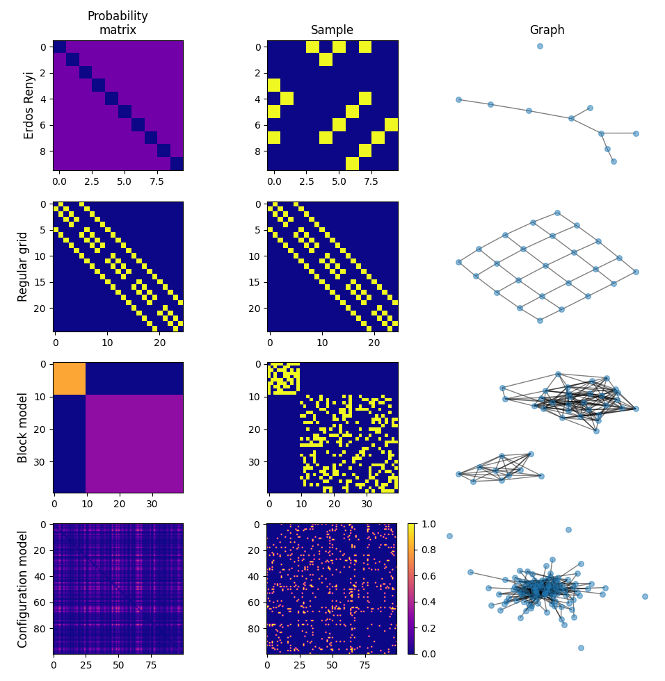
Figure 1: Initial conditions for simulations of the rewiring process. In each row, from left to right: A network probability matrix, a sample drawn from the same probability, and the graph representation of said sample. From top to bottom, an Erdös Rényi-Random graph, a 2 dimensional regular grid, a block model and a configuration model.

II.2 Watts-Strogatz Rewiring with variable number of links

It is also easy to extend this result beyond conservation of the number of links. First, consider that the left-hand-side of eq. 2 describes the change in the average number of links, which is $0$ for the case of conservation. For a value different from $0$, in which $\Delta c$ links are added and $\Delta a$ removed, the equation for the change of average number of links becomes

$$\sum_{i,j>i}p_{ij}(1,0)-p_{ij}(0,1)=\Delta c-\Delta a\,.$$ (14)

Next, we must keep in mind that the constraint on the Hamming distance between two successive measurements of the system is also affected by the change in the average number of links. The Hamming distance represents how many values in our network have changed in a single time-step. As we are considering the case where links are added, removed and rewired in such a way that the changes do not affect one another (they do not cancel each other out), the timescale constraint eq. 4 amounts to

$$\sum_{i,j>i}p_{ij}(1,0)+p_{ij}(0,1)=2+\Delta c+\Delta a\,.$$ (15)

With eq. 3 unchanged, the creation and annihilation probabilities become

$$c =\frac{1+\Delta c}{N(N-1)/2-L}$$ (16)

$$a =\frac{1+\Delta a}{L}\,.$$

This case is a “natural extension” of the results presented in the previous subsection because the functional form of the constraints does not change, only the value that they take. This is analogous to equilibrium entropy results where, for example, it is the functional form of the constraint on the total number of connections in a network that determines that the resulting ensemble is Erdös-Rényi, not the specific value of the number of links.

In order to compare to simulations of a modified rewiring process which allows the change of the average number of links, we will use the same initial conditions, evolution time and number of realisations as in the previous subsection (described in the previous subsection and shown in fig. 1). The difference is that, besides choosing a link that will be randomly placed between disconnected nodes, we will choose $\Delta a$ connected nodes to be removed and $\Delta c$ disconnected ones to be added (also uniformly at random without changes cancelling each other out) at each step of the rewiring process. We will first consider the case in which $\Delta a=0$ and $\Delta c=1$ every $\tau$ steps (otherwise, both are $0$), producing a linear increase in the average number of links. In this case, $\Delta a$ and $\Delta c$ take integer values, so they can be used for the entropic approach and the simulations. However, the entropic approach is constructed by an average over realisations, suggesting that $\Delta a$ and $\Delta c$ can take on real values (although for each step of the process the amount of created and annihilated links must still be integers). To test this, we will consider the case in which $\Delta a=\max(0,-\sin(\omega t))$ and $\Delta c=\max(0,\sin(\omega t))$, which give a periodic oscillation of the average number of links. The number of created and annihilated links used in individual steps of the simulations are then drawn from an exponential distribution with rate $\Delta a$ and $\Delta c$, which oscillate in time.

III Results and discussion

III.1 Conservation of the number of links

We will now compare the evolution of link probabilities resulting from simulations of the rewiring process to the results obtained from the maximum entropy perspective (for the case where the average number of links of the network is held constant). For this, we will show how the probability of particular links (that is, particular choices of $i$ and $j$) being active evolves over time according to the simulations and the entropy-based evolution.

We will first focus on the fixed-network initial conditions (i.e. those on the second and third columns of fig. 1), that is when realisations of the rewiring process start from the same initial network. As mentioned in section II, in this case the network adjacency matrix $X$ and the probability of connected links $p_{ij}(x_{o}=1)$ are the same. In fig. 2 we show, with circular markers, the evolution of the probability of an arbitrarily chosen link that starts out with probability $1$ (i.e. is initially connected) in orange and that of one that starts out with probability $0$ (i.e. is initially disconnected) in blue, according to simulations. In dashed lines we show the evolution of links with the same initial connection probabilities according to what is expected from maximum entropy, finding agreement between calculations and experiments for the different types of networks (Erdös Rényi: ER, regular grid: RG, block model: BM, and configuration model: CM). We have verified that other links starting with the same initial proabilities present the same evolutions as those shown (for each network), as expected by the creation and annihilation probabilities not depending on specific $i,j$ pairs.

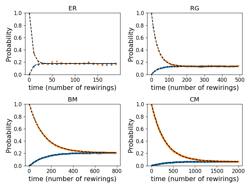
Figure 2: Probability of an initially connected link (orange) and an initially disconnected one (blue) according to simulations in circular markers and according to maximum entropy in dashed lines. Initial conditions correspond to the networks sampled from each probability matrix, shown in the second and third columns (from left to right) of fig. 1.

Next, in fig. 3, we show the evolution of the connection probability of specific links when ensemble-like initial conditions (i.e. the probability matrix in the first column of fig. 1) are used. In circular markers, each colour corresponds to links with initially different probability values (on average over realisations). The dashed lines correspond to the evolutions of links with the same initial probability according to maximum entropy results.

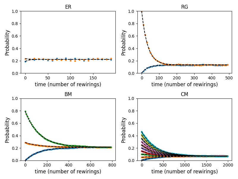
Figure 3: Probability of finding a link at selected pairs of nodes over time when initial conditions are sampled from the probability matrices shown in fig. 1 in each realisation of the rewiring process (in circular markers) and by applying the transition matrix found through maximum entropy to probability matrix (in dashed lines).

For example, the Erdös-Rényi random graph (ER, top left of fig. 3) draws samples which initially take link values that are either $0$ or $1$. On average over these samples, however, all links have the same probability of being connected, resulting in the curves in full lines (corresponding to specific pairs of links in the network) starting from the same probability. Additionally, because the Erdös-Rényi random graph is the equilibrium state of the rewiring process, the probability of connection over time stays constant. For the regular grid (RG), neighbouring nodes have a probability of $1$ of being connected while all others have probability $0$, so the observed evolution is identical to the one in fig. 2 . The block model takes three possible probability values, corresponding to connections within the small block, large block, or between them, resulting in the three different evolutions from the three possible initial probability values. Finally, the configuration model practically takes a continuum of initial probability values, so we have chosen $10$ links with approximately evenly spaced initial probabilities to compare their evolutions.

In both the case of sampled initial conditions and ensembles given by probability matrices, the evolution according to maximum entropy matches that of the simulations with high accuracy. This indicates that the method is well suited to replace realisations of dynamical processes on networks, yielding the distribution of trajectories based on given constraints analogously to how traditional maximum entropy methods yield the distribution of equilibrium states.

III.2 Variable number of links

We will now compare the evolution of link probabilities resulting from simulations of the rewiring process to the results obtained from the maximum entropy perspective, for the case where the average number of links in the network varies in some predefined way. We will show the evolution of the probability of specific links being connected, just as was shown in fig. 2 and fig. 3. However, as it has already been shown in the previous subsection that maximum entropy is equally suited for initial conditions that represent specific networks or ensembles of them, we will focus on the results of ensemble-type initial conditions (i.e. probability matrices shown in the first column of fig. 1). The chosen variations of the average number of links are linearly increasing and oscillating number of links (mentioned at the end of section II).

In fig. 4 we compare the evolution obtained from the average over simulation realisations (in circular markers) for different pairs of links in the network, to the evolution according to maximum entropy (in dashed lines). In this case, besides the rewiring described previously, the network adds a new link every $\tau$ time steps. Once again, the average over realisations of simulations is in very good agreement with the results from maximum entropy. Additionally, we note (especially for the Erdös-Rényi network and the random graph), that once the link probabilities have reached the same value, they continue this way (i.e. the system becomes quasi-static, meaning that it is described by the equilibrium distribution with time-dependent parameters).

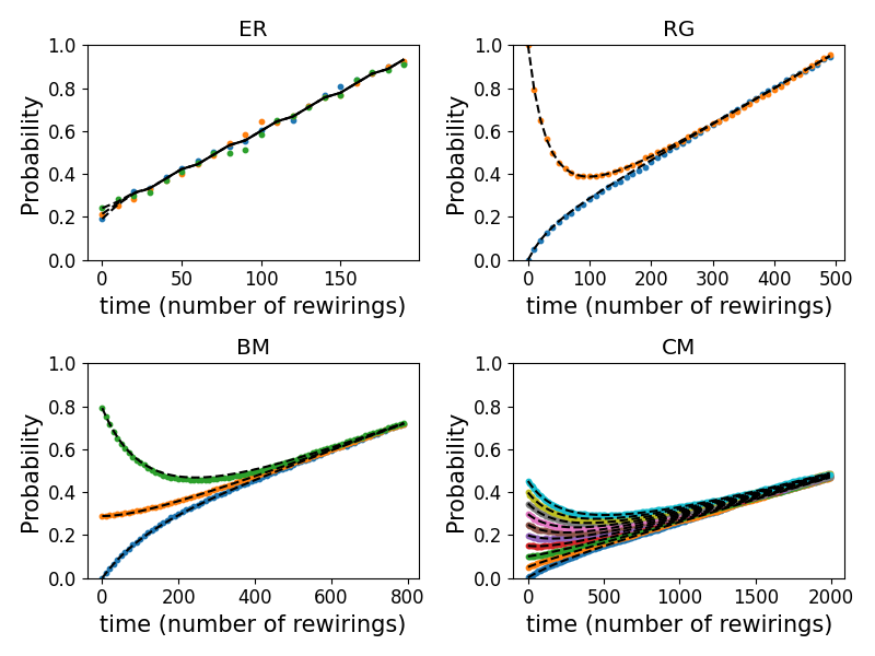
Figure 4: Evolution of link probabilities between selected pairs of nodes under linear increase of the average number of links. Circular markers show averages over realisations from ensemble-like initial conditions (i.e. probability matrices on the first column of fig. 1) while dashed lines show the evolution according to maximum entropy from the same initial conditions.

As mentioned in section II, adding (or removing) an integer amount of links is well defined for the simulations, but maximum entropy suggests that the change in the number of links may be defined on average. In fig. 5 we show the evolution of the linking probability of selected node-pairs when the number of links to be removed and added, at each time-step and in each realisation of the simulations, is drawn from an (integer) exponential distribution with time-dependent rates $\Delta c$ and $\Delta a$ (in full lines). In dashed lines, we show the evolution of the linking probability according to the creation and annihilation probabilities obtained by maximum entropy, where $\Delta c$ and $\Delta a$ are the rates used for drawing samples in the simulations. The agreement between simulations (in circular markers) and maximum entropy indicates that the method is well suited for describing dynamic processes, even when these do not reach a stationary distribution. The system reaches a quasi-static state (this time, oscillating in time) repeating the behaviour observed before now for the case of oscillatory dynamics.

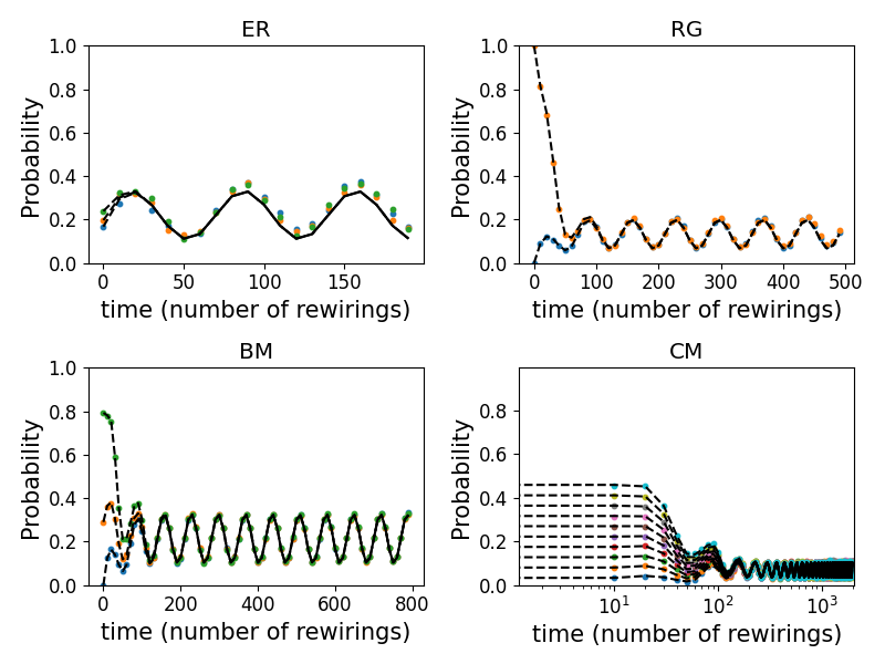
Figure 5: Evolution of linking probabilities for selected pairs of nodes from ensemble-like initial conditions (probability matrices shown in fig. 1) under oscillating average number of links. Results from simulations are shown with circular markers while maximum entropy is in dashed lines. The evolution of the configuration model is shown in logarithmic scale (in time) to make the transitory period more visible.

It should be noted that in these cases the dynamics of the average number of links $L(t)$ are set independently from maximum entropy. Just as in equilibrium, any value of $L$ can be chosen, for the dynamic perspective any $L(t)$ can be chosen. Initial conditions must be compatible with $L(0)$, and $\Delta a$ and $\Delta c$ must agree with, for example, the maximum number of links in the network (determined by the number of nodes). This means that the method presented here is an extension of equilibrium maximum entropy to dynamic processes in the sense that the average values in equilibrium are replaced by the dynamics of these averages, regardless of where they come from. In particular, if the averages are constant in time then the distribution converges to equilibrium result (in particular, remaining constant if the initial condition is the equilibrium state). Additionally, in both the time-dependent cases the ensemble distribution tends to a quasi-static evolution defined by the distribution corresponding to equilibrium (Erdös-Rényi) and properties matching the imposed average number of links. However, for some applications it may be more interesting to determine $\Delta a$ and $\Delta c$ as a function of, for example the number of links. A logistic growth could be modelled by simply imposing that $\Delta c-\Delta a=rL(M-L)$ and $\Delta a=0$, for example, but a better grounded approach would obtain this result from additional constraints, for example for the rates of link creation and destruction separately. Even though special attention was paid to the total number of links (because of its central role in the application of maximum entropy to networks), in appendix B we repeat our approach for a degree sequence-preserving process with maximum caliber.

III.3 Connection to maximum entropy production and entropic dynamics

From the results presented it is fairly clear that maximum caliber is able to provide a description of microscale transitions from macroscale constraints, analogously to equilibrium maximum entropy. Markov processes naturally arise when constraints can be described in terms of only two successive times along with marginalisation. For all practical purposes, in these cases we can maximise

$$S=-\sum_{x^{\prime},x}p(x^{\prime},x)\ln(p(x^{\prime},x))$$ (17)

subject to

$$\sum_{x^{\prime},x}f_{n}(x^{\prime},x)p(x^{\prime},x)= a_{n}$$ (18)

$$\sum_{x^{\prime}}p(x^{\prime},x)= p(x)$$

where $p(x)$ represents a known previous condition which starts out as the initial distribution and is updated by the result of the optimisation. This results in the two-step distribution which can be marginalised on the variable of the first step in order to obtain the updated condition. Since, for every step the optimisation holds $p(x)$ constant, we can also maximise the information entropy production

$$\Delta S =-\sum_{x^{\prime},x}p(x^{\prime},x)\ln(p(x^{\prime},x))+\sum_{x}p(x)\ln(p(x))$$ (19)

$$=-\sum_{x^{\prime},x}p(x^{\prime},x)\ln(p(x^{\prime},x)/p(x))$$

$$=-\sum_{x^{\prime},x}p(x^{\prime}|x)p(x)\ln(p(x^{\prime}|x))\,.$$

Note that the second equality is acheived by assuming marginalisation for the entropy of the initial distribution, which is valid as we are searching for the optimum of the entropy production in the subset of two-state distributions where this occurs. However, it is not imposed for all terms of the entropy production so it will still be included as a constraint.

As $p(x^{\prime}|x)$ is a (linear) matrix multiplication of $p(x^{\prime},x)$, we can maximise the entropy production with respect to the transition matrix instead of the two-step distribution, and subject to

$$\sum_{x^{\prime},x}f_{n}(x^{\prime},x)p(x^{\prime}|x)p(x) =a_{n}$$ (20)

$$\sum_{x^{\prime}}p(x^{\prime}|x) =1\,.$$

This defines a Lagrangian

$$\mathcal{L}= -\sum_{x^{\prime},x}p(x^{\prime}|x)p(x)\ln(p(x^{\prime}|x))$$ (21)

$$+\sum_{x}\lambda_{x}\left(1-\sum_{x^{\prime}}p(x^{\prime}|x)\right)$$

$$+\sum_{n}\lambda_{n}\left(a_{n}-\sum_{x^{\prime},x}f_{n}(x^{\prime},x)p(x^{\prime}|x)p(x)\right)$$

maximised by

$$\frac{\partial\mathcal{L}}{\partial p(x^{\prime}|x)}=0$$ (22)

$$=-p(x)\left[\ln(p(x^{\prime}|x)+1+\sum_{n}\lambda_{n}f_{n}(x^{\prime},x))\right]-\lambda_{x}$$

$$\Rightarrow p(x^{\prime}|x)=\exp\left(-\left[\lambda_{x}/p(x)+1+\sum_{n}\lambda_{n}f_{n}(x^{\prime},x)\right]\right)\,.$$

Imposing that $\sum_{x^{\prime}}p(x^{\prime}|x)=1$,

$$z_{x}: =\exp\left(\lambda_{x}/p(x)+1\right)=\sum_{x^{\prime}}\exp\left(-\sum_{n}\lambda_{n}f_{n}(x^{\prime},x)\right)$$ (23)

$$\Rightarrow p(x^{\prime}|x)=\frac{\exp\left(-\sum_{n}\lambda_{n}f_{n}(x^{\prime},x)\right)}{z_{x}}$$

$$\Rightarrow a_{n}=-\partial_{\lambda_{n}}\sum_{x}\ln(z_{x})p(x)$$

Note that the same functional form is obtained if the “entropy production” is written as $-\sum_{x^{\prime},x}p(x^{\prime}|x)\ln(p(x^{\prime}|x))$ and the constraints $\sum_{x^{\prime},x}f_{n}(x^{\prime},x)p(x^{\prime}|x)=b_{n}$ and $\sum_{x^{\prime}}p(x^{\prime}|x)=1$ (this is the case for entropic dynamics).

In order to establish a relation between constraints on the dynamics of average values (i.e. $\sum_{x^{\prime},x}f_{n}(x^{\prime},x)p(x^{\prime}|x)p(x)=a_{n}$) and those only on the transition matrix (i.e. $\sum_{x^{\prime},x}f_{n}(x^{\prime},x)p(x^{\prime}|x)=b_{n}$), consider that $z_{x}$ is valid for both approaches as long as the functional form of the constraints is the same. As $p(x)$ is independent from the multipliers, one can simply write $-\partial_{\lambda_{n}}\sum_{x}\ln(z_{x})=b_{n}$. This means that both approaches are equivalent as they differ only in the choice of how constraint values are defined.

IV Conclusions

In this work we have applied the principle of maximum caliber of Jaynes to construct dynamic network processes from imposed constraints. The method is an approach to constructing dynamic processes from maximum entropy in the same way that equilibrium states are obtained. We have focused on the total number of links in the network, obtaining the Watts-Strogatz rewiring process for the case when the amount of connections is held constant by the process. We have also shown the applicability beyond conservation by controlling changes in the amount of links over time, in both cases comparing the evolution to simulations from various initial conditions.

The main difference between the method presented here and other approaches of maximum caliber is the replacement of a normalisation condition over the whole trajectory of a variable with a marginalisation constraint, essentially imposing the history of a variable. With this perspective, other constraints on the system (beyond marginalisation) that can be written in terms of two successive states were found to naturally lead to Markov processes, and a connection to entropic dynamics was made.

As for future work, the specific choices of the constraints should be better understood in terms of their compatibility and sampling over time. Another path is the exploration of models for weighted networks. In particular, because equilibrium maximum entropy networks have been shown to be better reconstructed by imposing constraints on binary and weighted properties, such constraints might be applied to the interplay between structure generated by dynamical systems and dynamics on that structure. Finally, the marginalisation interpreted as an imposition of the “history” of a random variable suggests that this approach treats memory-dependent processes in a somewhat more similar manner to Markov processes than other approaches. We aim to use the method in the context of trajectory dependence, comparing it to other approaches, in future work.

Appendix A Maximum caliber and Markov processes

The prescription of maximum caliber is to associate to a path $\vec{X}_{T}:=(x_{o},x_{1},x_{2},...,x_{T})$ a probability $p(\vec{X}_{T})$, so the entropy of a path ensemble is

$$S=-\sum_{\vec{X}_{T}}p(\vec{X}_{T})\ln(p(\vec{X}_{T}))\,.$$ (24)

Constraints on $p$ can be written as

$$\sum_{\vec{X}_{T}}p(\vec{X}_{T})f_{n}(\vec{X}_{T})=a_{n}(T)$$ (25)

which are constraints on trajectories $\vec{X}_{T}$ of the evolution. For example, for the conservation of the number of links, the constraint is

$$\sum_{i,j>i}\sum_{\vec{X}_{T}}\left(\sum_{t=0}^{T}x_{t}\right)p_{ij}(\vec{X}_{T})=(T+1)L\,,$$ (26)

where $L$ is the average number of links at a fixed instant $t$ of the evolution of the network. Note that, subtracting two successive times $T$ and $T-1$, the result is an “instantaneous” constraint that depends only on the state of the network at $T$

$$\sum_{i,j>i}\sum_{\vec{X}_{T}}x_{T}p_{ij}(\vec{X}_{T})=\sum_{i,j>i}\sum_{x_{T}}x_{T}p_{ij}(x_{T})=L\,.$$ (27)

Therefore, according to [19] the process is Markov. Additionally, if we subtract the instantaneous constraint at two successive times we get the conservation constraint used in section II, i.e. $\sum_{i,j>i}\sum_{\vec{X}_{T}}(x_{T}-x_{T-1})p_{ij}(\vec{X}_{T})=0$. Note, however, that for the timescale constraint $\sum_{i,j>i}\sum_{\vec{X}_{T}}|x_{T}-x_{T-1}|p_{ij}(\vec{X}_{T})=2$ we cannot construct an instantaneous constraint that depends only on the state of the network at time $t$. However, the resulting process is still Markov as the constraint depends only on two successive times.

Finally, consider the case where the constraint on the average number of links over trajectories is modified to include a “memory” term, for example

$$\sum_{i,j>i}\sum_{\vec{X}_{T}}\left(\sum_{t=0}^{T}A_{T}e^{-t}x_{t}\right)p_{ij}(\vec{X}_{T})=(T+1)L\,,$$ (28)

where $A_{T}=(1-e^{-1})/(1-e^{-(T+1)})$ is a constant for each duration $T$ that normalises the weights $e^{-t}$ induced by the memory. When we attempt to construct the instantaneous constraint by difference of two successive times, we find that the resulting constraints again depend on the whole trajectory,

$$\sum_{i,j>i}\sum_{\vec{X}_{T}} \left[A_{T}e^{-T}x_{T}+\right.$$ (29)

$$~{}+\sum_{t=0}^{T-1}\left.(A_{T}-A_{T-1})e^{-t}x_{t}\right]p_{ij}(\vec{X}_{T})=L\,,$$

and the same is true for the corresponding conservation constraint, indicating that the resulting process is not Markov. Therefore being able to reduce constraints to depend only on the state of the system at a given instant is a sufficient condition to ensure that the resulting dynamics are Markov, but not a necessary one. Additionally, by constructing the transition matrix corresponding to the imposed constraints without assuming that the resulting process is Markov, the presented perspective on entropy maximisation for dynamic processes seems well suited for memory dependent and Markov processes alike.

Appendix B Maximum entropy degree-preserving rewiring

We will now repeat the same logic used to obtain the dynamics that conserve the number of links, only now conserving the degree sequence (the vector of in and out degrees of each node) of the network, not just its total number. We will also consider a directed network instead of an undirected one as for degree sequence constrained systems the constraints are clearer. For this, the marginalisation constraint is identical $\sum_{x_{T}}p_{ij}(\vec{X}_{T})=p_{ij}(\vec{X}_{T-1})$. The “minimal change” of a single step in the process (defining the timescale as in eq. 4 is now $\sum_{i,j}\sum_{\vec{X}_{T}}|x_{T}-x_{T-1}|p_{ij}(\vec{X}_{T})=4$, instead of to $2$ as two links are involved, each changing the value of two entries in the array of connections. Finally, instead of just one constraint on the total number of links in the network, we have $2N$ constraints, one for each in and out degree of each node. The Lagrangian is therefore

$$\mathcal{L}= S+\lambda_{ij\vec{X}_{T-1}}\left(p_{ij}(\vec{X}_{T-1})-\sum_{x_{T}}p_{ij}(\vec{X}_{T})\right)$$ (30)

$$+\lambda\left(4-\sum_{ij}\sum_{\vec{X}_{T}}|x_{T}-x_{T-1}|p_{ij}(\vec{X}_{T})\right)\,$$

$$+\sum_{i}\lambda^{out}_{i}\left(0-\sum_{j}\sum_{\vec{X}_{T}}(x_{T}-x_{T-1})p_{ij}(\vec{X}_{T})\right)$$

$$+\sum_{j}\lambda^{in}_{j}\left(0-\sum_{i}\sum_{\vec{X}_{T}}(x_{T}-x_{T-1})p_{ij}(\vec{X}_{T})\right)$$

yielding (by deriving the Lagrangian with respect to the distribution, finding the maximum as a function of the distribution, and then imposing marginalisation)

$$\rho_{ij} (x_{T}|x_{T-1})=$$ (31)

$$=\frac{\exp(-(\lambda^{out}_{i}+\lambda^{in}_{j})(x_{T}-x_{T-1})-\lambda|x_{T}-x_{T-1}|)}{\sum_{x}\exp(-(\lambda^{out}_{i}+\lambda^{in}_{j})(x-x_{T-1})-\lambda|x-x_{T-1}|)}$$

$$=\begin{pmatrix}1-c_{ij}&a_{ij}\\ c_{ij}&1-a_{ij}\\ \end{pmatrix}$$

$$=\begin{pmatrix}\frac{1}{1+\exp(-(\lambda^{out}_{i}+\lambda^{in}_{j}+\lambda))}&\frac{1}{1+\exp(-(\lambda^{out}_{i}+\lambda^{in}_{j}-\lambda))}\\ \frac{1}{1+\exp(\lambda^{out}_{i}+\lambda^{in}_{j}+\lambda)}&\frac{1}{1+\exp(\lambda^{out}_{i}+\lambda^{in}_{j}-\lambda)}\\ \end{pmatrix}$$

Differently from the Watts-Strogatz rewiring process, the transition matrix of each link is different (restrained to the dependence on the same $\vec{\lambda}^{out}$ and $\vec{\lambda}^{in}$). This makes imposing the conservation constraints extremely difficult to solve analytically (i.e. obtaining a relation between the multipliers and the imposed average values). However, as in the equilibrium case of imposing the degree of each node (the binary configuration model), this reduces the degrees of freedom in constructing the solution to the problem, and gives a functional form which can be adjusted numerically to the imposed constraint values.

A single step of the corresponding simulated process is carried out as follows. Out of all pairs of connected nodes in a given network, two connections $i,j$ and $k,l$ are selected randomly and uniformly. These pairs must be such that all nodes are different, $i$ and $l$ are not connected, and $j$ and $k$ are not connected. If a selected pair is not suitable, another is drawn, but this remains the same step of the process. Once a suitable pair is found, the connections $i,j$ and $k,l$ are removed and replaced by $i,l$ and $k,j$. This is a single step and is repeated to give individual realisations, and the distribution of trajectories on these realisations is studied just as for the processes described in section II. In fig. 6 we show the evolution of connection probabilities over time according to the simulations and maximum entropy, for $5$ pairs of nodes from the fixed-network initial conditions shown in the second and third columns of fig. 1.

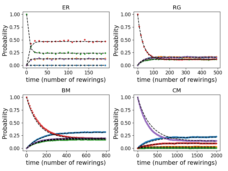
Figure 6: Probability of $5$ different pairs of nodes of being connected as a function of time (number of steps) comparing results from simulations and maximum entropy.

The most notable difference between this case and Watts-Strogatz rewiring is that, as the connection probabilities can evolve differently for each pair of nodes, trajectories can start from the same point and still behave differently. There is also a larger difference (due to the number of realisations required) between the simulation (full lines) and maximum entropy (dashed lines) results. We have verified that the stationary connection probability values achieved by individual links (the asymptotic values of fig. 6) agree with the distribution expected by the directed binary configuration model, $p_{ij}\rightarrow(1+\exp(\alpha_{i}+\beta_{j}))^{-1}$ such that $\sum_{i}p_{ij}=k^{\text{in}}_{j}$ and $\sum_{j}p_{ij}=k^{\text{out}}_{i}$ (defined by the in and out degree of the initial network respectively). This again suggests that the distributions resulting from traditional entropy maximisation correspond to equilibrium distributions of a dynamic process defined by the same constraints as equilibrium, but defining transition matrices for the probability distribution instead of the distribution itself.

References

- Bertz [1981] S. H. Bertz, The first general index of molecular complexity, Journal of the American Chemical Society 103, 3599 (1981).
- Abadi and Ruzzenenti [2023] N. Abadi and F. Ruzzenenti, Complex networks and interacting particle systems, Entropy 25, 1490 (2023).
- Pedersen et al. [2021] T. T. Pedersen, M. Victoria, M. G. Rasmussen, and G. B. Andresen, Modeling all alternative solutions for highly renewable energy systems, Energy 234, 121294 (2021).
- Merz et al. [2023] E. Merz, E. Saberski, L. J. Gilarranz, P. D. Isles, G. Sugihara, C. Berger, and F. Pomati, Disruption of ecological networks in lakes by climate change and nutrient fluctuations, Nature Climate Change 13, 389 (2023).
- Farahani et al. [2019] F. V. Farahani, W. Karwowski, and N. R. Lighthall, Application of graph theory for identifying connectivity patterns in human brain networks: a systematic review, frontiers in Neuroscience 13, 585 (2019).
- Note [1] On the other hand, in cases where links take on more than two possible values, for example , and or even a continuous range , the network is classified as weighted.
- Note [2] Otherwise it is called directed.
- Newman [2003] M. E. Newman, Mixing patterns in networks, Physical review E 67, 026126 (2003).
- Dadashi et al. [2010] M. Dadashi, I. Barjasteh, and M. Jalili, Rewiring dynamical networks with prescribed degree distribution for enhancing synchronizability, Chaos: An Interdisciplinary Journal of Nonlinear Science 20 (2010).
- Bertotti and Modanese [2020] M. L. Bertotti and G. Modanese, Network rewiring in the r-k plane, Entropy 22, 653 (2020).
- Garlaschelli and Loffredo [2008] D. Garlaschelli and M. I. Loffredo, Maximum likelihood: Extracting unbiased information from complex networks, Physical Review E 78, 015101 (2008).
- Squartini et al. [2011a] T. Squartini, G. Fagiolo, and D. Garlaschelli, Randomizing world trade. i. a binary network analysis, Physical Review E 84, 046117 (2011a).
- Squartini et al. [2011b] T. Squartini, G. Fagiolo, and D. Garlaschelli, Randomizing world trade. ii. a weighted network analysis, Physical Review E 84, 046118 (2011b).
- Squartini and Garlaschelli [2017] T. Squartini and D. Garlaschelli, Maximum-entropy networks: Pattern detection, network reconstruction and graph combinatorics (Springer, 2017).
- Note [3] Which may not be the case for arbitrarily defined randomisation steps.
- Watts and Strogatz [1998] D. J. Watts and S. H. Strogatz, Collective dynamics of ‘small-world’networks, nature 393, 440 (1998).
- Barabási and Albert [1999] A.-L. Barabási and R. Albert, Emergence of scaling in random networks, science 286, 509 (1999).
- Jaynes [1980] E. T. Jaynes, The minimum entropy production principle, Annual Review of Physical Chemistry 31, 579 (1980).
- Ge et al. [2012] H. Ge, S. Pressé, K. Ghosh, and K. A. Dill, Markov processes follow from the principle of maximum caliber, The Journal of chemical physics 136 (2012).
- Pressé et al. [2013] S. Pressé, K. Ghosh, J. Lee, and K. A. Dill, Principles of maximum entropy and maximum caliber in statistical physics, Reviews of Modern Physics 85, 1115 (2013).
- Dixit et al. [2018] P. D. Dixit, J. Wagoner, C. Weistuch, S. Pressé, K. Ghosh, and K. A. Dill, Perspective: Maximum caliber is a general variational principle for dynamical systems, The Journal of chemical physics 148 (2018).
- Ghosh et al. [2020] K. Ghosh, P. D. Dixit, L. Agozzino, and K. A. Dill, The maximum caliber variational principle for nonequilibria, Annual review of physical chemistry 71, 213 (2020).
- Davis and González [2015] S. Davis and D. González, Hamiltonian formalism and path entropy maximization, Journal of Physics A: Mathematical and Theoretical 48, 425003 (2015).
- Caticha [2011] A. Caticha, Entropic dynamics, time and quantum theory, Journal of Physics A: Mathematical and Theoretical 44, 225303 (2011).
- Caticha [2015] A. Caticha, Entropic dynamics, Entropy 17, 6110 (2015).
- Pessoa et al. [2021] P. Pessoa, F. X. Costa, and A. Caticha, Entropic dynamics on gibbs statistical manifolds, Entropy 23, 494 (2021).
- Cover [1999] T. M. Cover, Elements of information theory (John Wiley & Sons, 1999).
- Note [4] In general the link is moved with probability , but we will fix for simplicity.
- Note [5] Assuming .
- Note [6] The Hamming distance between two matrices is understood to be the sum of the Hamming distances between corresponding rows.
- Note [7] Note that this constraint is sensible to the choice of in the probability of actually replacing a link. In general the right hand side of eq. 4 is .
- Note [8] Note that the link cannot be placed in the position from which it was removed in order for the Hamming distance constraint to be valid.
- Note [9] This is the same as interpreting the specific samples drawn to obtain the results of fig. 2 as binary probability matrices.