Accelerating Material Property Prediction using Generically Complete Isometry Invariants

Abstract

Material or crystal property prediction using machine learning has grown popular in recent years as it provides a computationally efficient replacement to classical simulation methods. A crucial first step for any of these algorithms is the representation used for a periodic crystal. While similar objects like molecules and proteins have a finite number of atoms and their representation can be built based upon a finite point cloud interpretation, periodic crystals are unbounded in size, making their representation more challenging. In the present work, we adapt the Pointwise Distance Distribution (PDD), a continuous and generically complete isometry invariant for periodic point sets, as a representation for our learning algorithm. While the PDD is effective in distinguishing periodic point sets up to isometry, there is no consideration for the composition of the underlying material. We develop a transformer model with a modified self-attention mechanism that can utilize the PDD and incorporate compositional information via a spatial encoding method. This model is tested on the crystals of the Materials Project and Jarvis-DFT databases and shown to produce accuracy on par with state-of-the-art methods while being several times faster in both training and prediction time.

1 Introduction

A crystalline structure is made up of a repeating arrangement of atoms. Crystals can distinguish themselves by both the species of atoms they contain as well as how these atoms are structured. Both of these aspects can determine the various properties of a crystal. Knowledge of these properties is pertinent for determining whether a crystal can be experimentally synthesized or is useful for a particular application.

Determination of property values can be done using ab initio calculations with techniques like density functional theory (DFT) (Sholl & Steckel, 2011) or force field levels (Niketic & Rasmussen, 2012). These techniques can vary in accuracy and are often computationally expensive (Cohen et al., 2012). In some cases, prohibitively so. Further, they require extensive domain knowledge to be applied to even a single crystal, making them inaccessible. This has resulted in a search for alternative methods. In recent years, machine learning has become very popular for this task and has experienced success in decreasing computational costs while producing accurate predictions.

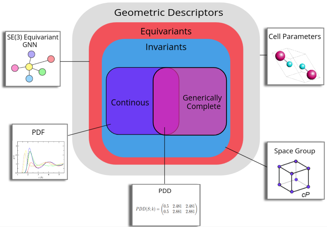
Figure 1: Classification of geometric descriptors for periodic crystals based on the properties possessed. Cell parameters consist of the unit cell lengths and angles, but this is ambiguous as there are an infinite number of unit cells. Space group is a label defined by the symmetry relations the crystal exhibits, but is sensitive to atomic perturbations. Equivariant GNNs cannot be used to distinguish periodic structures. PDF needs additional smoothing to retain continuity, introducing more parameters. The PDD is invariant, generically complete and continuous under EMD.

Any application of machine learning requires the adaptation of a data representation that adequately describes the object of interest and is compatible with the algorithm being used. Objects similar to crystals, like molecules and proteins, are often treated as finite point clouds. This makes their representation more easily constructible than a representation for crystals, which are not bounded in size. Further, while a crystal can be described in several ways, descriptors that are easily human-interpretable, such as unit cell parameters or atomic coordinates are not useful for machine learning algorithms. Atomic coordinates, for instance, do not retain invariance under rigid motion. Unit cell based descriptors are also ambiguous as there are an infinite number of valid unit cells for any given periodic crystal.

The structure-property relationship (Le et al., 2012) dictates that changes in the structure of a material result in changes in its properties. Distinction between crystals then allows for distinction between their respective property values. Fundamentally, a machine learning algorithm (for a regression task) is a mapping from representation to value. If a representation cannot distinguish periodic crystals then two different crystals can incorrectly be perceived to be the same and so will the output property values. Similarly, if the same crystal can be represented in different ways, mapping to the same value cannot be guaranteed.

Isometry invariants can be effective representations for crystal structures depending on their properties. Crystals are treated as periodic point sets that are unordered and span infinitely Smith & Kurlin (2022). Two periodic point sets $S$ and $Q$ are isometric if there exist bijective isometries $f:S\rightarrow Q$ and $g:Q\rightarrow S$ such that $f(S)=Q$ and $g(Q)=S$. An isometry $f$ is a distance preserving map between metric spaces satisfying $d({\bm{s}}_{i},{\bm{s}}_{j})=d(f({\bm{s}}_{i}),f({\bm{s}}_{j}))$ for any ${\bm{s}}_{i},{\bm{s}}_{j}\in S$ and a valid metric $d$. Since crystals are treated as point clouds these isometries include those that fall under rigid motion: translation, rotation, and reflection. An isometry invariant I is a property (descriptor or function) that is preserved under any isometry. This representation is often simpler than the initial object, for example, a scalar, vector, or matrix. Not all invariants can be considered equally useful, however. Space groups, for example, reflect the symmetry of a given material but tiny changes in atomic positioning caused by perturbations can change the material’s space group. While this is enough to distinguish two crystals, no indication is given of how different they are. Figure 1 illustrates the relationship between geometric descriptors based on their properties. An invariant should possess the following qualities described by (Widdowson & Kurlin, 2022, Problem 1.1)

Problem 1.

Find a function $I$ on all periodic point sets in $R^{n}$ subject to the following conditions:

1. Invariance: If two periodic point sets, $S$ and $Q$ are isometric, then $I(S)=I(Q)$.

2. Completeness: If $I(S)=I(Q)$, then the two periodic sets are isometric.

3. Metric: There exists a distance function $d$ on the codomain $I$ that satisfies the following: 1) $d(I(S),I(Q))=0$ iff $I(S)=I(Q)$. 2) $d(I(S),I(Q))=d(I(Q),I(S))$. 3) For any three periodic sets $S,Q,$ and $T$, $d(I(S),I(Q))+d(I(Q),I(T))\geq d(I(S),I(T))$

4. Lipschitz continuity: If a periodic set $Q$ is obtained by shifting points within periodic set $S$ by at most $\epsilon$, then the distance between the two periodic sets can be bound according to $d(I(S),I(Q))\leq C\epsilon$ for some fixed constant $C$.

5. Computability: For any periodic set S, the value $I(S)$ can be computed in polynomial time with respect to the size of the motif of $S$.

6. Reconstructibility: The periodic set $S$ can be fully reconstructed from its invariant $I(S)$.

In the present work, we will use an isometry invariant called the Pointwise Distance Distribution (PDD) which has properties $1.1a$ through $1.1e$, and satisfies $1.1f$ for any periodic set in the general position (Widdowson & Kurlin, 2022). The PDD, defined formally in Definition 2.2, is invariant, generically complete, and has an established continuous metric using the Earth Mover’s Distance (Rubner et al., 2000). It can also be constructed in near-linear time, making its application to large datasets feasible.

The main contribution of this work is a model based on the transformer architecture (Vaswani et al., 2017) which utilizes the PDD of a crystal to make predictions on the properties of materials in a highly efficient manner compared to state-of-the-art models. In doing this, we bridge the gap between unambiguous crystal descriptors and machine learning models. We show that such a representation is effective in producing results that are on par or better than graph-based models, despite the additional structuring of data that comes in the form of edges and edge embeddings. Further, this model is shown to be several times faster in both prediction and training speed compared to two state-of-the-art models. To provide evidence of the method’s robustness, the model is applied to the crystals of the Materials Project (Jain et al., 2013) and Jarvis-DFT (Choudhary et al., 2020).

Early works in crystal property prediction used more classical statistical methods like kernel regression (Calfa & Kitchin, 2016) before eventually moving towards deep learning (Ye et al., 2018). More recent works have shifted to Graph Neural Networks (GNN) (Xie & Grossman, 2018; Choudhary & DeCost, 2021; Yan et al., 2022; Omee et al., 2022; Park & Wolverton, 2020; Chen et al., 2019; Das et al., 2022; Cheng et al., 2021; Sanyal et al., 2018; Schütt et al., 2018) due to their ability to make use of structured data. Several of these focus on predicting the properties of the crystals contained within the Materials Project (Jain et al., 2013) using a multigraph representation where vertices represent atoms and edges are embedded with the pairwise distances to an atom’s nearest neighbors. Some state-of-the-art models use line graphs to incorporate more geometric information like angles and dihedrals (Choudhary & DeCost, 2021; Ruff et al., 2023). The derived line graphs can contain significantly more vertices and edges, incurring a higher computational cost. Lin et al. (2023) take a physics principled approach and substitute the interatomic distances for interatomic potentials and capture a crystal’s periodicity using the infinite sum of these potentials.

While graphs are effective in modeling crystal structures, they are discontinuous under perturbations (Edelsbrunner et al., 2021). Small movements in the atomic positioning can cause significant changes to the graph’s topology. Some graphs also rely on the choice of unit cell. Due to an infinite number of possible unit cells, the graph is then reliant on the data or the cell reduction technique used.

Equivariant (Thomas et al., 2018) models are a step in the right direction when compared to those that rely on non-invariant geometric descriptors. Even so, invariance is a stronger and thus, more desirable property than equivariance. Invariant representations are required for distinguishing between crystals, while equivariant representations cannot be relied upon to do so. Equivariant transformers have been developed for finite points clouds (Fuchs et al., 2020), but the periodic case has yet to be handled. Equivariant GNNs are still limited by discontinuity and reliance on the unit cell Du et al. (2022); Xie et al. (2021).

Many invariants for crystal structures exist, but there are few with all the desired properties. Smooth Overlapped Atomic Positions (Bartók et al., 2013) and Atomic Cluster Expansion (Drautz, 2019) for example, are both invariants, but due to the reliance on a finite subset of the periodic set, lack continuity. The Pair Distribution Function (PDF) (Terban & Billinge, 2021) uses X-Ray Diffraction Patterns for distinguishing crystals, but cannot differentiate homometric structures (Patterson, 1939). Further, the PDD is a stronger invariant than the PDF as the PDF requires smoothing to recover continuity (Widdowson & Kurlin, 2022, Section 3).

In addition to the properties mentioned earlier, the invariant needs to be able to be adapted for a machine learning algorithm. Further, it needs a way to incorporate compositional information as invariants typically only consider structure. Some invariants have been adapted for use in machine learning algorithms such as symmetry functions (Behler, 2011; Egorova et al., 2020) and Voronoi cells (Ward et al., 2017). Both of these, however, still lack continuity. The Partial Radial Distribution Function is invariant and continuous but is not complete for homometric crystals. Average Minimum Distance (AMD) (Widdowson et al., 2022) is invariant and continuous and has been used to predict lattice energies via Gaussian Process Regression (Ropers et al., 2022), but does not have a way to incorporate compositional information.

2 Methods

We can define a crystal more generally in terms of a periodic point set (Smith & Kurlin, 2022) or periodic set for short.

Definition 2.1 (Periodic Point Set).

For a set of $n$ basis vectors ${\bm{v}}_{1}\ldots{\bm{v}}_{n}\in\mathbb{R}^{n}$, the lattice $L$ is formed by the integer linear combinations of these basis vectors $\{\sum_{i=1}^{n}c_{i}{\bm{v}}_{i}|c_{i}\in\mathbb{Z}\}$. The unit cell is the parallelepiped $U=\{\sum_{i=1}^{n}t_{i}{\bm{v}}_{i}|t_{i}\in[0,1)\}$. For a unit cell $U$, the motif $M$ is a finite subset of $U$. Then, a periodic point set $S$ of lattice $L$ and motif $M$ is defined by $\{\bm{\lambda}+{\bm{p}}:\bm{\lambda}\in L,{\bm{p}}\in M\}$.

The PDD of a periodic set is the $m\times(k+1)$ matrix where $m$ is the number of atoms in the motif $M$ and $k$ is a positive integer indicating the number of nearest neighbors to use. Each row corresponds to a point in the motif and the entries within the row consist of the Euclidean distance to each of this point’s $k$-nearest neighbors within the entire periodic set $S$. The first entry of the row is assigned to be a weight equal to $\frac{1}{m}$ (the distances follow). Once the matrix is formed, rows that are the same are collapsed into a single row and their respective weights are added. Due to very small differences between rows caused by floating point arithmetic or atomic perturbations, it is common to use a tolerance, henceforth called the collapse tolerance, that allows rows with small non-zero differences (e.g. with respect to $L_{\infty}$ distance) to be treated as the same. By collapsing rows in the PDD, the resulting matrix representation is always the same for a given crystal, regardless of the unit cell. Formally,

Definition 2.2 (Pointwise Distance Distribution).

For a periodic set $S=L+M$ with a set of motif points $M=\{{\bm{p}}_{1},\ldots,{\bm{p}}_{m}\}$ within a unit cell $U$ of lattice $L$, the uncollapsed PDD matrix for a parameter $k\in\mathbb{N}^{+}$ is a $m\times(k+1)$ matrix where the $i^{th}$ row consists of the row weight $w_{i}=\frac{1}{m}$ followed by the euclidean distances $d_{1}\ldots d_{k}$ from the point ${\bm{p}}_{i}$ to its $k$-nearest neighbors such that $d_{1}\leq d_{2}\ldots\leq d_{k}$. If a group of rows is found to be identical (or close enough using a valid distance measure within some tolerance) then the matrix rows are collapsed and the weights of the involved rows are summed. The resulting matrix will then have less than $m$ rows. The rows of the matrix are finally ordered lexicographically. This matrix is referred to as $\textsc{PDD}(S;k)$ for a periodic set $S$ and positive integer $k$.

2.1 Periodic Set Transformer

In our model, rather than being considered a matrix of values, the PDD will be considered a set of grouped atoms. A single group of atoms corresponds to the $k$-nearest neighbor distances in a given row within the PDD matrix. Each member of the set will carry the weight provided by the row in the PDD. Any set $A$ can trivially be turned into a weighted set by weighing each element by $\frac{1}{|A|}$. When the PDD is not collapsed, then there can be more than a single occurrence of any given element, making the uncollapsed PDD a multiset. Now, let $A$ be a multiset of the form $A=\{a_{i}^{(j)}:i\in[1,\dots,n],j\in[1,\dots,n_{i}]\}$ where $n_{i}$ is the multiplicity of element $a_{i}$ and $a_{i}^{(j)}$ is the $j^{th}$ occurrence of element $a_{i}$. This multiset can be turned into a weighted set by assigning each element $a_{i}$ with the weight $\frac{n_{i}}{n}$. We can recover the influence of multiplicity by the use of weights in our model.

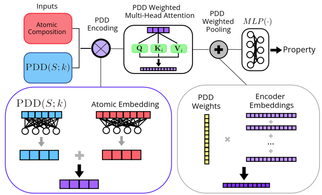
Figure 2: Overview of the architecture of the Periodic Set Transformer. PDD encoding is used to combine the structural information in the PDD with atomic types. The weights of the PDD are incorporated in the attention mechanism and during the pooling of the embeddings to define the multiplicity of the input set.

When a periodic crystal has its unit cell modified, the proportion of each atom is expanded or reduced. The use of weights captures this behavior in the form of a concentration or frequency. In this way, we can describe a potentially arbitrarily large crystal structure in terms of a distribution consisting of the atoms within a crystal that exhibit a particular behavior.

We use an attention mechanism to find the interactions between members of the set. The rows of the PDD contain the pairwise distance information, but they do not indicate which atoms these distances correspond to. Application of the attention mechanism can help the model learn these interactions.

Let ${\bm{R}}\in\mathbb{R}^{m\times k}$ be the PDD matrix containing $m$ rows without the associated weight column. Let ${\bm{w}}\in\mathbb{R}^{m\times 1}$ be the column vector containing the weights from the PDD matrix. The initial embedding is ${\bm{X}}^{(0)}={\bm{R}}{\bm{W}}_{d}$ where ${\bm{W}}_{d}\in\mathbb{R}^{k\times d}$ is the initial trainable weight matrix. The embedding is updated according to:

$${\bm{X}}^{(1)}={\bm{X}}^{(0)}+SLP\Bigg{(}\sigma\left(\frac{{\bm{Q}}{\bm{K}}^{T}}{\sqrt{d}}\right){\bm{V}}\Bigg{)}$$ (1)

where ${\bm{Q}}={\bm{X}}^{(0)}{\bm{W}}_{Q}$, ${\bm{K}}={\bm{X}}_{i}^{(0)}{\bm{W}}_{K}$ and ${\bm{V}}={\bm{X}}^{(0)}{\bm{W}}_{V}$ and $d$ is the embedding dimension of the weight matrices for the query, key, and value ${\bm{W}}_{Q},{\bm{W}}_{K},$ and ${\bm{W}}_{V}$ respectively as described in Vaswani et al. (2017). The function $\sigma$ is the softmax function with the PDD weights integrated into it; $\sigma$ is applied to each row ${\bm{z}}$ of the input matrix, and $i$ and $j$ are used to index entries in ${\bm{z}}$ and ${\bm{w}}$. The $i^{th}$ entry of the output vector is defined by:

$$\sigma({\bm{z}})_{i}=\frac{w_{i}e^{z_{i}}}{\sum_{j=1}^{m}w_{j}e^{z_{j}}}$$ (2)

The result is passed through a single-layer perceptron $SLP$. The layer normalization order described by Xiong et al. (2020) is used for increased stability during training. Equation 2 describes the case for a single attention head. When multiple attention heads are used, the PDD weights are applied to each individually and the result is concatenated before being passed to the SLP like so:

$${\bm{X}}^{(1)}={\bm{X}}^{(0)}+SLP\Bigg{(}\bigoplus_{i=1}^{h}\sigma\left(\frac{{\bm{Q}}_{i}{\bm{K}}_{i}^{T}}{\sqrt{d}}\right){\bm{V}}_{i}\Bigg{)}$$ (3)

where $h$ is the number of attention heads, $\oplus$ is the concatenation operator and ${\bm{Q}}_{i},{\bm{K}}_{i}$ and ${\bm{V}}_{i}$ are the query, key and value for the $i^{th}$ head. This process is repeated $l$ times; this determines the depth of the model. The embeddings are finally pooled into a single vector by reincorporating the PDD weights into a weighted sum of the row vectors ${\bm{x}}_{i}$ of the final embedding ${\bm{X}}^{(l)}$.

$${\bm{x}}=\sum_{i}w_{i}{\bm{x}}_{i}$$ (4)

This final embedding can be passed to a perceptron layer to predict the property value.

This is similar to dot product attention as defined by the original Transformer article (Vaswani et al., 2017), but it is a modified version of self-attention that incorporates the PDD weights, though it is not limited to this. This version of self-attention can be applied to a weighted set or distribution. The weights are applied in such a way that the output of the PST is invariant to an arbitrary splitting of rows within the PDD. We provide a formal proof of this in supplementary material Section A.

An overview of the Periodic Set Transformer (PST) architecture with PDD encoding (described in the next section) can be seen in Figure 2.

2.2 PDD Encoding

While structure is a powerful indicator of a crystal’s properties, there may be datasets in which it is not the primary differentiator of a set of crystals. In such cases, the composition of the atoms contained within the material has a heavy influence. The previously described transformer does a good job of utilizing the structural information within the PDD but does not provide an obvious way to include atomic composition. Here we will describe a method to incorporate this information while maintaining all benefits of the PDD.

Transformers for natural language processing tasks use positional encoding to allow the model to distinguish the position of words within a given sentence (Dufter et al., 2022). A recent transformer model, Uni-Mol (Zhou et al., 2023), which performed property prediction for molecules (among other tasks), used 3D spatial encoding first proposed by Ying et al. (2021) to give the model an understanding of each atom’s position in space, relative to one another. This encoding is done at the pair level, using the Euclidean distance between atoms and a pair-type aware Gaussian kernel (Shuaibi et al., 2021). A transformer model for finite $3D$ points clouds is provided by Zhao et al. (2021) via vector attention. The case for crystals is more difficult because they are not bounded in size and encoding at the pair level can result in discontinuity under perturbations. Fortunately, by using the rows of the PDD we can distinguish each atom with structural information. We refer to this as PDD encoding.

When rows are grouped together, they are done so by having the same $k$-nearest neighbor distances. Though rare, it is possible for rows corresponding to different atom types to be collapsed. If this occurs, the selection of either atom type will result in information loss. To prevent this, we add the condition that the groups must be formed on the basis of having the same $k$-nearest neighbor distances and the same atomic species. In this case, the periodic point set has points that are labeled according to atomic type.

For a periodic set $S$, let $PDD(S;k)$ be the resulting PDD matrix with parameter $k$. Let ${\bm{R}}$ be $PDD(S;k)$ without the initial weight column and ${\bm{T}}$ be the matrix whose rows correspond to the vector of atomic properties used to describe the type of atom associated with each row of $PDD(S;k)$. The initial set of embeddings for the attention mechanism is defined as ${\bm{X}}^{(0)}={\bm{R}}{\bm{W}}_{s}+{\bm{T}}{\bm{W}}_{c}$ where ${\bm{W}}_{s}$ and ${\bm{W}}_{c}$ are initial embedding weights. By starting with a linear embedding, the PDD row can be transformed to match the dimension of composition embedding. The parameter $k$ used can then be changed as needed to include distance information from further neighbors. As with positional encoding, we displace the atomic embedding by the PDD encoding vector by summing. The rest of the model continues as before.

3 Results and Discussion

3.1 Prediction of Materials Project Properties

The model will be applied to the data within the Materials Project. To make fair comparisons to other models we report the performance according to Matbench (Dunn et al., 2020), which contains data for various crystal properties. The error rates are reported using five-fold cross-validation with standardized training and testing sets for each fold. Further, tuning is done according to the models’ authors and thus our model can be compared to others more fairly. The hyper-parameters and training options for the PST are listed in Table 1.

The crystals in the Materials Project are highly diverse in composition. For all predictions, we include the composition of the crystal with PDD encoding. To incorporate this compositional information the mat2vec atom embeddings supplied by Tshitoyan et al. (2019) are used. The embeddings have empirically been found to produce better performance than the one-hot encoded method used by CGCNN (Wang et al., 2021). They also have the added convenience of not missing any atomic property information for certain elements.

Table 1: Hyper-parameters for the Periodic Set Transformer when applied to the Matbench datasets.

Hyper-parameter	Value
Attention Head Size	128
Number of heads	4
Encoders	4
Dropout	0.0
Attention dropout	0.1
Batch Size	32/64
Weight decay	$10^{-5}$
$k$	15
Collapse Tol.	$10^{-4}$
Epochs	250

In Table 2 we report the average mean-absolute-error (MAE) across the five test sets. We include the reported accuracies of other models to allow for comparison. The selection of models aims to present a high diversity in approaches while also coming from relatively recent publications. CrabNet (Wang et al., 2021) is the only other Transformer model listed on Matbench. This model, in terms of architecture, is the most similar to the PST. Additionally, the atomic embeddings used to describe each chemical element are the same as those used in our model. The majority of models used in crystal property prediction use GNNs. Matbench features several of these, but the model that provides the best results on several properties is coGN. coGN is a GNN that includes angular and dihedral information through the use of line graphs. As such, the amount of information used is significantly more than the PST, which uses only pairwise distances. Crystal Twins (CT) (Magar et al., 2022) is a model based on the convolutional layer developed by CGCNN (Xie & Grossman, 2018) (also used by several other models (Choudhary & DeCost, 2021; Cao et al., 2023; Das et al., 2022)) that uses self-supervised learning to create embeddings based on maximizing the similarity between augmented instances of a crystal.

Table 2: Five-fold cross-validation prediction MAE and standard deviation of MAE for properties of the crystals in the Materials Project. Bold values indicate the best (lowest) error rate while underlined values indicate the second-best error rate. PST performance is reported using PDD Encoding with a tolerance of $10^{-4}$ and $k=15$.

Property	Units	PST	CrabNet	coGN	CrystalTwins
Formation Energy	$eV/atom$	0.032 $\pm$ 0.0003	0.086 $\pm$ 0.001	0.021 $\pm$ 0.0003	0.037 $\pm$ 0.001
Band Gap Energy	$eV$	0.210 $\pm$ 0.002	0.266 $\pm$ 0.003	0.156 $\pm$ 0.002	0.264 $\pm$ 0.011
Shear Modulus	$log_{10}(GPa)$	0.074 $\pm$ 0.001	0.101 $\pm$ 0.002	0.069 $\pm$ 0.001	0.086 $\pm$ 0.004
Bulk Modulus	$log_{10}(GPa)$	0.056 $\pm$ 0.003	0.076 $\pm$ 0.003	0.053 $\pm$ 0.003	0.067 $\pm$ 0.003
Refractive Index	n/a	0.290 $\pm$ 0.078	0.323 $\pm$ 0.071	0.309 $\pm$ 0.086	0.417 $\pm$ 0.080
Phonon Peak	$1/cm$	29.40 $\pm$ 1.40	57.76 $\pm$ 5.73	29.71 $\pm$ 1.99	48.86 $\pm$ 7.69
Exfoliation Energy	$meV/atom$	31.15 $\pm$ 9.566	45.61 $\pm$ 12.24	37.16 $\pm$ 13.68	46.79 $\pm$ 19.92
Perovskites FE	$eV$	0.030 $\pm$ 0.001	0.406 $\pm$ 0.007	0.027 $\pm$ 0.001	0.042 $\pm$ 0.001

The PST and CrabNet share similarities in their construction. Both use mat2vec atomic embeddings and utilize a Transformer architecture with self-attention. While CrabNet uses fractional encoding to embed the multiplicity of each element type, we opt for the PDD-weighted attention mechanism and pooling described by Equations 2 and 4. The PST also uses PDD encoding to add structural information. This could also be done for CrabNet, but the combination of both fractional and PDD encoding is not guaranteed to aid in performance and simple summation of the encodings can cause ambiguities in the final embeddings, reducing performance. Across all properties the PST outperforms CrabNet, further indicating the usefulness of PDD encoding.

The root cause of the disparity in prediction accuracy between the PST and coGN on formation and band gap energy can be difficult to discern. GNNs allow embeddings at the vertex and edge level. In certain models, these embeddings can not only carry different information but allow for simultaneous updates to each of these embeddings, adding richness to the learned representation. CoGN takes this a step further and updates the original edges with message-passing from the derived line graph, allowing the inclusion of angular information. The edges of the line graph are further updated by its line graph, incorporating dihedral angles. These updates allow the model to learn a better representation of a crystal in latent space, which can be necessary for these larger datasets. This points to a current limitation for the PST. By using PDD encoding, we effectively limit opportunities for such updates to a single embedding representing both the atom’s properties and its structural behavior.

In Table 3 the time taken to train and test the PST and coGN are listed. Our model was trained for only 250 epochs while coGN is trained for 800 epochs. While this accounts for a large portion of the disparity, the time taken to train each model per epoch is also faster for our model in all properties except refractive index. A batch size of 32 is used for datasets containing less than $5,000$ samples. For exfoliation energy and phonon peak, PST takes $68.1\%$ and $92.6\%$ of the time of coGN per epoch. The larger batch size of coGN allows it to have greater GPU utilization and thus, better training efficiency. For properties with greater than $5,000$ samples, the batch size for both models is the same. For these properties, the training time per epoch is between $65-70\%$ of coGN.

The prediction time disparity is more pronounced. As the number of samples grows the difference in prediction speed lessens, but is still significant. For band gap and formation energy, the PST makes predictions approximately five times faster than coGN. Using nested line graphs introduces significant computational cost, but coGN is able to shrink the size of the initial graph by using the atoms in the asymmetric unit instead of the atoms in the unit cell. The unit cell based approach was initially proposed by CGCNN (Xie & Grossman, 2018) and used in several follow-up works (Das et al., 2022; Park & Wolverton, 2020; Choudhary & DeCost, 2021; Magar et al., 2022), but the unit cell is inherently ambiguous and unnecessarily large in terms of the number of atoms needed to fully describe a crystal’s symmetry. The PDD at a collapse tolerance of exactly zero will have a number of rows less than or equal to the number of atoms in the asymmetric unit. At higher tolerances, this number will be reduced until reach the number of unique chemical elements in the crystal. Such an increase in the tolerance can further speed up training and prediction time, though it is possible that this results in a decrease in prediction accuracy as information loss occurs. This is further investigated in Section D.2.

Table 3: Single-fold prediction (measured in seconds) and training time (measured in minutes) for the PST (using $k=15$ and a collapse tolerance of $10^{-4}$) and coGN (Ruff et al., 2023) on Matbench (Dunn et al., 2020). Training and prediction was done using an Nvidia RTX 3090. Time does not include evaluation of the models on the validation sets or data pre-processing times.

Property	Samples	Training Time (min.)		Prediction Time (sec.)
		PST	coGN	PST	coGN
Formation Energy	132,752	159.1	772.1	2.79	15.25
Band Gap	106,113	126.6	602.1	2.38	11.88
Perovskites	18,928	13.41	62.37	0.31	2.93
Bulk Modulus	10,987	8.47	42.24	0.23	1.99
Shear Modulus	10,987	8.38	41.23	0.22	2.05
Refractive Index	4,764	6.89	20.23	0.12	1.29
Phonon Peak	1,265	1.81	6.25	0.04	0.87
Exfoliation Energy	636	0.89	4.18	0.02	0.79

3.1.1 Ablation Study

In Table 4 we list the results for each ”component” within the Periodic Set Transformer. In the row indicating PDD as the component, we train and test the model using only the structural information within the PDD. In the ”Composition” component we pass the atomic encoding for the elements in the crystal and their concentration in the form of the PDD weights to the model without the PDD encoding. The model is run using $k=15$ and a collapse tolerance of exactly zero.

By separating out each component of the model, we can interpret the importance of each to a particular property. Properties that experience a more significant decrease in performance when the PDD encoding is not used, can be ascribed to be more dependent on structural information. In all cases, the combination of both the composition and PDD encoding results in significantly lower error rates. We can conclude that this encoding method is effective in combining the structural and compositional information of a crystal structure.

Table 4: Effect of PDD encoding on prediction MAE of the Materials Project crystals. Results are separated by input components where ”Composition” uses only the mat2vec atomic embeddings (Tshitoyan et al., 2019) and ”PDD” uses only the PDD. Errors in bold indicate the best performance and underlined errors indicate second-best performance (lower is better $\downarrow$).

Property (units)	Component MAE $\downarrow$
	Composition	PDD	PST
Band Gap   $(eV)$	0.273	0.596	0.212
Formation   $(eV)/atom$	0.088	0.421	0.032
Shear Modulus   $log_{10}(GPa)$	0.107	0.132	0.075
Bulk Modulus   $log_{10}(GPa)$	0.080	0.115	0.055
Refractive Index	0.352	0.451	0.292
Phonon Peak   $1/cm$	50.39	74.71	27.75
Exfoliation   $(meV)/atom$	46.91	39.35	31.55
Perovskites   $(eV)/atom$	0.621	0.393	0.030

In Table 5 the effect of including the PDD weight in the attention mechanism described in Equation 2 and in the pooling layer described by Equation 4 is listed. A collapse tolerance of zero is used to remove any regularization effect (further described in Section D.2).

As expected, the exclusion of weights from both the attention mechanism and pooling decreases accuracy significantly. Doing this removes all indications of multiplicity making discernment of crystals more difficult. The inclusion of the weights in the pooling layer is more impactful than when applied in the attention mechanism. The use of the weights in the pooling layer alone allows the model to perform better when the number of samples in the dataset is low. Datasets with fewer samples likely have less diversity amongst their crystals, making the need for recognizing the multiplicity of atoms less necessary.

Table 5: Effect of including the PDD weights as defined by Equations 2 and 4 on prediction MAE of the Materials Project crystals. Results for ”No weights” use mean pooling and a normal softmax function. Errors in bold indicate the best performance and underlined errors indicate second-best performance (lower is better $\downarrow$).

Property (units)	PDD Weight Inclusion MAE $\downarrow$
	No Weights	Attention Only	Pooling Only	PST
Band Gap   $(eV)$	0.278	0.244	0.219	0.212
Formation   $(eV)/atom$	0.045	0.037	0.035	0.032
Shear Modulus   $log_{10}(GPa)$	0.080	0.077	0.076	0.075
Bulk Modulus   $log_{10}(GPa)$	0.059	0.059	0.056	0.055
Refractive Index	0.314	0.284	0.288	0.292
Phonon Peak   $1/cm$	31.02	28.84	27.96	27.75
Exfoliation   $meV/atom$	35.59	32.52	31.83	31.55
Perovskites   $(eV)/atom$	0.031	0.030	0.031	0.030

3.2 Prediction of Jarvis-DFT Properties

The Jarvis-DFT dataset (Choudhary et al., 2020) is a commonly used set of materials with VASP (Kresse & Furthmüller, 1996) calculated properties. The list of properties computed for the materials within the dataset is more extensive than that of the Materials Project. Its inclusion provides further evidence of the robustness of the model on an even wider variety of crystal properties.

Table 6: Hyper-parameters for the Periodic Set Transformer when applied to the Jarvis-DFT materials dataset.

Hyper-parameter	Value
Attention Head Size	128
Number of heads	4
Encoders	4
Dropout	0.0
Attention dropout	0.1
Batch Size	64
Weight decay	$10^{-5}$
$k$	15
Collapse Tol.	$10^{-4}$
Epochs	250

The prediction MAE produced by PST and Matformer for $12$ different properties from the dataset are included in Table 7. For Matformer, we retrain the model to ensure the training and testing sets are the same. We use the default parameters for the model defined by the authors’ codebase. We make one alteration to the training procedure; the number of epochs trained is reduced to 250. The number of epochs is the same as for our model. The hyper-parameters used for the PST when applied to the Jarvis-DFT dataset are listed in Table 6.

Table 7: Prediction MAE on the properties of the Jarvis-DFT dataset using the PST and Matformer. Results for Matformer Yan et al. (2022) are included for comparison. PST uses PDD encoding with $k=15$ and a collapse tolerance of $10^{-4}$. Bolded values indicate the best performance. Mean-absolute-deviation (MAD) of the test set is included.

Property	Units	Samples	Test MAD	PST	Matformer
Formation Energy	$eV/atom$	55,723	0.87	0.047	0.033
Band Gap (OPT)	$eV$	55,723	0.99	0.172	0.150
Total Energy	$eV/atom$	55,723	1.78	0.051	0.036
Ehull	$eV$	55,371	1.14	0.052	0.072
Bulk Modulus	$GPa$	19,680	52.80	10.76	11.70
Shear Modulus	$GPa$	19,680	27.16	9.523	10.13
Band Gap (MBJ)	$eV$	18,172	1.79	0.289	0.304
Spillage	-	11,377	0.52	0.367	0.373
SLME (%)	-	9,068	10.93	4.61	4.712
Max. piezo. stress coeff $(e_{ij})$	$Cm^{-2}$	4,799	0.26	0.127	0.243
Max. piezo. strain coeff $(d_{ij})$	$CN^{-1}$	3,347	24.57	13.09	18.03
Exfoliation Energy	$meV/atom$	813	62.63	30.91	55.04

The PST outperforms Matformer in nine of the twelve properties tested. In particular, properties for which data is sparse yield results that favor the PST significantly (i.e. exfoliation energy, $e_{ij}$ and $d_{ij}$). Jarvis-DFT has two band gap values that are computed for its crystals, one which uses the optimized Becke88 functional (OPT) (Klimeš et al., 2009) and the other uses the Tran-Blaha modified Becke Johnson potential (MBJ)Tran & Blaha (2009). The latter is more accurate (when compared to experimentally observed values) but also more computationally expensive. For this reason, there are significantly fewer computed values in the database. Interestingly, the PST produces a smaller error for the more accurate band gap values compared to Matformer, but a larger error for the less accurate OPT calculated values. A possible reason for this is the smaller sample size for which the PST has shown to be more effective. The disparity in performance for formation and total energy can be attributed to Matformer’s architecture which uses a GNN that updated both node and edge embeddings. This additional level of expression is helpful particularly when the size of the data grows larger, though it does come with added computational cost.

Matformer has been shown to produce even better results than the previous state-of-the-art model ALIGNN (Choudhary & DeCost, 2021) while taking roughly a third of the time to do both training and prediction. In Table 8, the training and prediction time for each of the properties in the Jarvis-DFT dataset is reported for the PST and Matformer. For the training time, the validation and pre-processing times are not included. The prediction time listed is the number of seconds taken to make predictions on the test set.

Table 8: Prediction (measured in seconds) and training time (measured in minutes) for the PST and Matformer (Yan et al., 2022) on Jarvis-DFT datasets. Training and prediction was done using an Nvidia RTX 3090. Time does not include evaluation of the models on the validation sets or data pre-processing times.

Property	Samples	Training Time (min.)		Prediction Time (sec.)
		PST	Matformer	PST	Matformer
Formation Energy	55,723	41.36	345.8	0.329	29.77
Band Gap (OPT)	55,723	41.62	343.9	0.347	29.86
Total Energy	55,723	41.65	349.1	0.349	29.79
Ehull	55,371	40.69	348.9	0.352	28.93
Bulk Modulus	19,680	14.12	93.33	0.135	11.12
Shear Modulus	19,680	14.45	93.70	0.123	10.69
Band Gap (MBJ)	18,172	13.38	118.7	0.107	9.71
Spillage	11,377	5.74	70.8	0.066	6.01
SLME (%)	9,068	4.62	58.75	0.055	4.82
Max. piezo. stress coeff $(e_{ij})$	4,799	3.52	23.15	0.029	2.57
Max. piezo. strain coeff $(d_{ij})$	3,347	2.44	15.38	0.026	1.79
Exfoliation Energy	813	0.63	5.30	0.008	0.41

In the closest training time comparison, the PST is still more than six times faster than Matformer. The training times for all properties fall between six and twelve times faster for the PST compared to Matformer. The performance increase can be attributed to several factors. Primarily, Matformer relies on a line graph (similar to coGN Ruff et al. (2023)) in order to update edge embeddings. While this increases the information used and leads to richer learned embeddings, the size of line graphs is considerably larger than the graph they are derived from. This, in turn, incurs a higher computational cost.

The difference in prediction times is more significant. Exfoliation energy is predicted over fifty times faster using the PST than with Matformer. This is the closest the two models perform to each other. Notably, exfoliation energy also has the fewest samples. For the bulk of the other properties, the speedup ranges between eighty and ninety times faster for the PST.

4 Conclusion

The PDD is a representation for periodic crystals which is invariant to rigid motion and independent of unit cell. By using weights and creating a distribution, the PDD is able to represent an infinitely spanning object by its finite forms of behavior. Further, by collapsing rows in the PDD, the resulting representation can also be much smaller in comparison to the number of atoms within the unit cell, even when the cell is reduced.

The model is applied to the crystals of the Materials Project and Jarvis-DFT on a variety of material properties. Despite using less information in the model than more commonly employed graph-based models, the PST is able to produce results on par or even exceeding that of models like coGN and Matformer while taking significantly less time to train and make predictions.

In future work, we would like to explore how pre-training can improve prediction results. Uni-Mol (Zhou et al., 2023) uses pre-training with a transformer for molecules which was shown to be very effective. The case for crystals is more complex as the number of atoms is not bounded. Pre-training tasks like pairwise distance and coordinate prediction are no longer viable without modifications to fit the periodic case. Regardless, because the PDD establishes a continuous metric on periodic sets for measuring structural differences, we believe it can be integrated into a pre-training task involving structure prediction.

Author Contributions

JB proposed the original model, VK proposed the spatial encoding method used. JB developed and tested the codebase used for the experiments. JB, VZ and VK contributed in writing the first draft of the article and subsequent revisions were completed by all three authors.

Competing Interests

All authors declare no financial or non-financial competing interests.

Data Availability

The data from the Materials Project is automatically downloaded through the code in the supplementary material. The Jarvis-DFT data can be downloaded through the Jarvis-Tools python package using the dft_3d_2021 database. Examples are included in the documentation here: https://pages.nist.gov/jarvis/databases/. The dataset for the crystals used in the lattice energy experiments is available at https://eprints.soton.ac.uk/404749/.

Code Availability

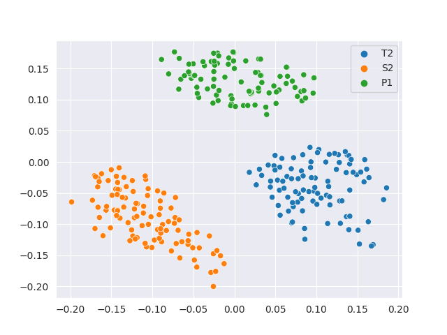
(a) MDS of sampled data by crystal type

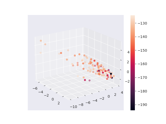
(b) MDS of T2 crystals

Figure 4: Multi-dimensional scaling projection on to $\mathbb{R}^{2}$ and $\mathbb{R}^{3}$ for the pairwise distances of crystals between each other. Subfigure (a) projects three types of crystals using distances created by using the Earth Mover’s Distance between PDDs for $k=10$. Subfigure (b) is created using the MDS projection of pairwise distances between PDDs at $k=100$ for one hundred random samples from the T2 crystals colored by lattice energy measured in kJ/mol.

The code for the experiments is located at https://github.com/jonathanBalasingham/Periodic-set-transformer. The code contains what is necessary to re-run the experiments done in sections C and 3.1. It also contains the source code necessary to recreate Figures 4(a) and 4(b). Details of how these plots are created are included in section B. The individual predictions for the Materials Project data are contained in JSON format within the repository. Proofs for the properties of the PDD mentioned in (Widdowson & Kurlin, 2022, Problem 1.1) are included in the original paper Widdowson & Kurlin (2022). More details on the actual implementation of the model, data pre-processing, and training are contained in section E.

Appendix A Equivalence of Distributions in the PST

If a PDD is arbitrarily expanded or collapsed, the PST should produce the same results as these PDDs are considered equivalent. The same can be said of any input distribution. This is proven here:

Lemma A.1.

Let $A$ and $B$ be weighted multisets each containing elements from the set $S=\{{\bm{x}}_{1},\ldots{\bm{x}}_{n}\}$. Each element ${\bm{x}}_{i}\in\mathbb{R}^{1\times n}$ occurs with multiplicity $m_{i}^{(a)}\in\mathbb{N}^{+}$ and $m_{i}^{(b)}\in\mathbb{N}^{+}$ in $A$ and $B$ respectively. Each element also carries weight $w_{i}^{(a)}\in\mathbb{R}^{+}$ and $w_{i}^{(b)}\in\mathbb{R}^{+}$ for $A$ and $B$ respectively. The application of the Periodic Set Transformer will yield equivalent output if

$$w_{i}^{(a)}m_{i}^{(a)}=w_{i}^{(b)}m_{i}^{(b)},\hskip 14.22636pt\forall i\in\{1,\ldots,n\}$$ (5)

Proof.

To prove that the output of the PST is equivalent for $A$ and $B$, it is sufficient to prove that the output of $\sigma$ (defined in Equation 2) and the pooling layer (defined in Equation 4) are the same for $A$ and $B$. Let ${\bm{q}}_{i}={\bm{x}}_{i}{\bm{W}}_{Q}$, ${\bm{k}}_{i}={\bm{x}}_{i}{\bm{W}}_{K}$, and ${\bm{v}}_{i}={\bm{x}}_{i}{\bm{W}}_{V}$ be the query, key, and value vectors produced by the weight matrices ${\bm{W}}_{Q},{\bm{W}}_{K},{\bm{W}}_{V}\in\mathbb{R}^{n\times d}$. First, note the pre-softmax attention weight from ${\bm{x}}_{i}$ to ${\bm{x}}_{j}$ can expressed as:

$$a_{ij} =\frac{{\bm{q}}_{i}{\bm{k}}_{j}^{T}}{\sqrt{d}}$$ (6)

and is independent of both weight and multiplicity. Further, notice that the summation of an expression over $A$ or $B$ can be rewritten using its multiplicities. For $A$ this is done like so:

$$\sum_{t=1}^{|A|}(\cdot)=\sum_{s=1}^{n}m_{s}^{(a)}(\cdot)$$

Using this equivalence, the function $\sigma$, used to calculate the attention weight from ${\bm{x}}_{i}$ to ${\bm{x}}_{j}$ for $A$ and ${\mathbb{B}}$, is written as:

$$\alpha_{ij}^{(a)} =\frac{w_{i}^{(a)}exp(a_{ij})}{\sum_{k=1}^{n}w_{k}^{(a)}m_{k}^{(a)}exp(a_{ik})}$$ (7)

and

$$\alpha_{ij}^{(b)} =\frac{w_{i}^{(b)}exp(a_{ij})}{\sum_{k=1}^{n}w_{k}^{(b)}m_{k}^{(b)}exp(a_{ik})}$$ (8)

Using the condition provided by Equation 5, Equation 8 can be rewritten as:

$$\alpha_{ij}^{(b)} =\frac{w_{i}^{(b)}exp(a_{ij})}{\sum_{k=1}^{n}w_{k}^{(a)}m_{k}^{(a)}exp(a_{ik})}$$ (9)

$$\sum_{k=1}^{n}w_{k}^{(a)}m_{k}^{(a)}exp(a_{ik}) =\frac{w_{i}^{(b)}exp(a_{ij})}{\alpha_{ij}^{(b)}}$$ (10)

Substituting back into Equation 7 gives us:

$$\alpha_{ij}^{(a)} =\alpha_{ij}^{(b)}\frac{w_{i}^{(a)}exp(a_{ij})}{w_{i}^{(b)}exp(a_{ij})}$$ (11)

$$\alpha_{ij}^{(a)} =\alpha_{ij}^{(b)}\frac{w_{i}^{(a)}}{w_{i}^{(b)}}$$ (12)

The attention weights produced from $A$ can now be expressed in terms of the attention weights produced from $B$. The $j^{th}$ entry in the attention vector for ${\bm{x}}_{i}$ in $A$ is:

$$y_{ij}^{(a)} =\sum_{j=1}^{n}\alpha_{ij}^{(a)}m_{j}^{(a)}v_{ji}$$ (13)

$$=\sum_{j=1}^{n}\alpha_{ij}^{(b)}\frac{w_{i}^{(a)}}{w_{i}^{(b)}}m_{j}^{(a)}v_{ji}$$ (14)

$$=\sum_{j=1}^{n}\alpha_{ij}^{(b)}\frac{w_{i}^{(a)}}{w_{i}^{(b)}}\bigg{(}\frac{w_{i}^{(b)}m_{i}^{(b)}}{w_{i}^{(a)}}\bigg{)}v_{ji}$$ (15)

$$=\sum_{j=1}^{n}\alpha_{ij}^{(b)}m_{i}^{(b)}v_{ji}$$ (16)

$$=y_{ij}^{(b)}$$ (17)

Thus, the resulting embeddings from the attention mechanism are equivalent. While the embeddings themselves are equivalent, the cardinality for each embedding still differs according to each multisets’ multiplicity. The pooling described by Equation 4 fixes this. Let ${\bm{z}}_{i}$ be the final embedding for ${\bm{x}}_{i}$. The output vector ${\bm{z}}$ from the pooling for $A$ is the sum:

$${\bm{z}}^{(a)} =\sum_{i=1}^{n}w_{i}^{(a)}m_{i}^{(a)}{\bm{z}}_{i}$$ (18)

Substituting Equation 5 again we get,

$${\bm{z}}^{(a)} =\sum_{i=1}^{n}w_{i}^{(b)}m_{i}^{(b)}{\bm{z}}_{i}$$ (19)

$$={\bm{z}}^{(b)}$$ (20)

Thus, the output of the PST for both $A$ and $B$ are equivalent. ∎

Appendix B Applications of the Pointwise Distance Distribution

In definition 2.2 we provided a formal definition for the PDD. Here, we will begin by providing an example of its construction.

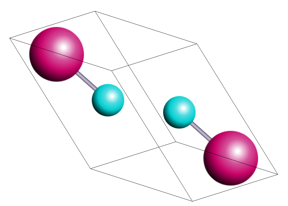
Figure 3: The unit cell of Lutetium-Silicon; Silicon is colored in teal and Lutetium in magenta.

Consider Lutetium-Silicon which is shown in Figure 3. The unit cell pictured contains a total of four atoms, 2 of which are Lutetium and 2 of which are Silicon. If we use $k=2$ nearest neighbors, the PDD matrix of this periodic set $S$ before rows are grouped is

$$PDD(S;k)=\begin{pmatrix}0.25&2.481&2.481\\ 0.25&2.481&2.481\\ 0.25&2.881&2.881\\ 0.25&2.881&2.881\end{pmatrix}$$

where the first column contains the weights for each row (atom). The second is the distance to the nearest neighbor and the third, the distance to the second nearest neighbor. The first two rows are identical, as are the final two. Because of this, each of the two groups of rows can be grouped into a single row as so,

$$PDD(S;k)=\begin{pmatrix}0.5&2.481&2.481\\ 0.5&2.881&2.881\end{pmatrix}$$

The rows are already lexicographically ordered so this is the finalized PDD. If a different unit cell is selected, this collapsing of matrix rows will continue to yield the same result as the proportion of each atom will not change.

The PDDs of two periodic crystals can be compared using the Earth Mover’s Distance (Rubner et al., 2000). The weights of each PDD can be considered the distribution we are comparing in the minimum flow problem. We can visualize a set of crystals by projecting these distances onto a two or three-dimensional plane.

Subfigure 4(a) shows the projection of the pairwise distances of the PDDs of one hundred samples from each of the three crystals in this experiment using Multi-Dimensional Scaling (MDS). This technique attempts to map a set of pairwise distances to specific $n$-dimensional space by minimizing the difference between the actual pairwise distances and the distances between the points in the projected space. Even with this error, we are able to establish three distinct clusters in two-dimensional space according to their respective crystal type.

Subfigure 4(b) shows the projection of the pairwise distances between the crystals’ PDD onto three-dimensional space for the T2 dataset. The colors of the points in each plot signify the lattice energy for the crystal. The distinction here is not as pronounced; this is to be expected as the sampled crystals are much more similar in their structure and thus the distances between the PDDs are smaller. Nonetheless, there is a discernible trend, and crystals that congregate near each other do share similar lattice energies.

Appendix C Prediction of Lattice Energy

Here, the dataset considered contains simulated molecular crystals created by Pulido et al. (2017) during the crystal structure prediction using quasi-random sampling (Case et al., 2016). This data is subsetted by the underlying molecule, e.g. T2. During structure prediction, crystals are generated while traversing the potential energy surface and their lattice energy is calculated using DMACRYS (Price et al., 2010) to determine their stability.

Prediction of lattice energy is done in three different scenarios. In the first, the model will be applied to a single set of molecular crystals with the same composition using $80/10/10$ training, validation, and testing splits. Next, the model is applied to multiple sets of crystals each with different underlying molecules using the same splits. The final experiment consists of the application of the model to a set of crystals with an underlying molecule it has not seen in training. The seen data is split $90/10$ for training and validation. To make predictions the PST described in section 2.1 is used with only the PDD as input and no knowledge of the composition.

Invariants are usually used to discern crystals by measuring differences between their structure. Here, the goal is to demonstrate the effectiveness of using an invariant as a representation for a machine learning algorithm. Even when compositional information is not present, the PDD can distinguish crystals with the EMD from the changes in the pairwise distances that occur when the species of atoms are changed. Whether the same distinction can be made in the context of a learning algorithm has previously not been shown.

We make a comparison to another invariant that has been used to predict lattice energy. Average-minimum-distance (Widdowson et al., 2022) was used as input for a Gaussian regression model (Ropers et al., 2022). In Table 9 we list the performance on the test set of this AMD model to allow comparison between invariants.

Our model reduces the mean-absolute-error (MAE) rate by $21\%$ compared to the Gaussian Process Regression technique which utilizes AMD (Ropers et al., 2022). The mean-absolute percentage error (MAPE) is also reduced by $1.63\%$. While we use $k=60$ nearest neighbors for constructing the PDD, the AMD model uses $k=500$ to achieve its best results. Despite the use of this additional information, the model using the PDD still performs more accurately.

In the second row of Table 9 we list the results of the second experiment. The previous task is extended to a dataset of crystals that contains different underlying molecules. These molecules have different compositions. This compositional information is not contained within the PDD (and thus, not in our input). The model will have to discern crystals solely by their structure. While the overall MAE has increased slightly, the percentage error has decreased. The domain on which the lattice energies lie is different for each type of crystal. Using the PDD alone is enough for the algorithm to distinguish the crystal types and predict lattice energy accordingly.

Table 9: Results of lattice energy prediction using the PDD with the PST and AMD with Gaussian regression on three different tasks using $80/10/10$ training, validation, and testing splits. (a) uses only experimentally generated structures of the T2 molecular crystal based on triptycene. (b) adds two additional sets of molecular crystals, P1 (based on pentiptycene) and S2 (based on spiro-biphenyl). (c) uses P1, P1M (methylated analogue of P1) and P2 (benzimidazolone series pentiptycene) in the training and validation set using a $90/10$ split. The test set consists only of P2M, the methylated analogue of P2.

	Train	Train Size	Test	Test Size	Invariant	MAE (kj/mol) $\downarrow$	MAPE $\downarrow$
(a)	T2	4,630	T2	578	AMD	4.79	4.31%
					PDD	3.76	2.68%
(b)	T2, P1, S2	14,547	T2, P1, S2	1,819	AMD	4.68	2.83%
					PDD	4.11	2.52%
(c)	P1,P1M,P2	22,995	P2M	7,352	AMD	12.99	6.89%
					PDD	7.24	3.89%

The final experiment uses the data from the P1, P1M, and P2 crystals in the training and validation data. The test set consists of the P2M crystal, which is not part of the either training or validation set. This experiment is the closest to real-world conditions in which new crystals often arise and finding the stable forms is crucial, but information on their lattice energy is unavailable.

When lattice energy is calculated using ab initio calculations, the range of the energies varies from crystal to crystal. When introducing a new type of crystal for our algorithm to make predictions on, this can become a problem as extrapolation to unvisited parts of the lattice energy range can result in high error rates. Fortunately, lattice energies between different types of crystals, are not usually meant to be compared. Instead, they are generated for potential polymorphs of a crystal in an effort to find those with the highest stability for synthesis. We can make use of this fact when applying our model to novel crystals. It is not necessary to predict the correct range of lattice energies; instead, the model needs to be able to predict the lattice energies of the various structures such that their ordering according to their lattice energy is correct. This task could feasibly be turned into a learning-to-rank problem (Liu et al., 2009), but as a regression task, it allows for a more general approach since the predicted lattice energies can be ordered after the fact.

Each dataset has its lattice energies shifted by the mean lattice energy towards zero. By doing this they each maintain their distribution but now overlap around the origin. The model is trained and validated based on this shifted data. The MAE of the predictions on the test set after they have been shifted back is $7.24$ kJ/mol and the MAPE is $3.89\%$.

While the MAE and MAPE are higher than in previous experiments, the improvement over AMD is more significant. The majority of errors come from underestimating the lattice energy. The datasets tend to grow sparser in these areas where lattice energy is lower as this is where the most stable structures tend to lie. Having a false positive (predicting a higher energy structure to be lower) increases the number of potentially stable structures. False negatives are more impactful as they may result in a structure not being considered entirely due to its seemingly low stability.

The histogram in Figure 5(a) shows the lattice energies (in kJ/mol) of the three crystals within the dataset. Figure 5(b) shows the comparison of the predictions of the model against the ground truth values.

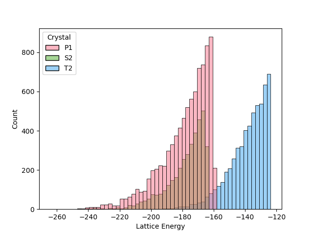
(a) Distribution of ground truth lattice energies.

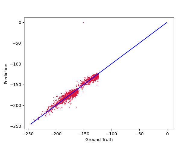
(b) Ground truth lattice energy vs. predictions

Figure 5: (a) The distribution of the lattice energies of the T2, S2 and P1 crystals. (b) The predictions of T2, S2, and P1 compared to the ground truth lattice energies in kJ/mol.

Predictions that have lower errors will have their point placed closer to the line colored in blue. The bulk of the points share their error both below and above the true lattice energy as we would expect in a model without bias. There are a few outliers, in particular, a single crystal from the T2 dataset has a predicted lattice energy of just $-0.41$. Prevention of such errors can be mitigated by using a different loss function than MAE. In particular, mean-squared error (MSE) and Huber loss can hedge against outlying errors by increasing their contribution to the loss function. We choose to not present the results using these loss functions as MAE still provides better results for MAE and MAPE.

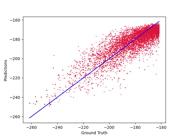
(a) Ground Truth vs. Predictions re-scaled according to mean.

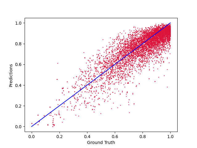
(b) Ground Truth vs. Predictions normalized between zero and one.

Figure 6: (a) Comparison of predictions vs. ground truth of the test set after the predictions are scaled back by the mean of the lattice energies. (b) The comparison of predictions vs. ground truth after both have been normalized between zero and one.

In Figure 6(a) we plot the original predictions on P2M after they have been re-scaled back away from the mean lattice energy. In Figure 6(b), we re-scale the prediction and the ground truth values to between zero and one. By doing this, we can see the ordering of the predictions compared to the true lattice energies. The scatter plot in Figure 6(b) allows us to compare lattice energies relative to other predictions.

If the error rate produced by the final experiment of section C is inadequate, we can supplement the training with predictions from classical methods. For a novel crystal, ab initio calculations can be used to generate lattice energies for a small subset of structures. These samples can be integrated into the training set to improve the overall results. In order to make this practical, we can only produce lattice energies for a limited portion of structures; we limit this to $10\%$ (or under) of the total structures.

Table 10: Effect of including portions of the P2M data into the training set on prediction accuracy.

Samples	Percent of P2M Data	Test MAE (kj/mol) $\downarrow$	Test MAPE $\downarrow$
0	0%	7.24	3.89%
367	5%	5.82	3.17%
735	10%	5.50	3.02%

Table 10 displays the result of adding this supplemental data to the training set. As expected, the addition of data decreases MAE and MAPE. Even with as few as $367$ samples (or $5\%$ of the total dataset), the reduction in error is significant. This process experiences diminishing returns as the amount of the original dataset is used in the training set. Though the MAE and MAPE continue to decrease, it is questionable whether or not spending time generating the instances using classical methods is worth the additional performance gains.

Appendix D Additional Experiments

D.1 Effect of $k$-nearest neighbors

PDD encoding can be said to be parameterized by two values, the collapse tolerance and the number of $k$-nearest neighbors. The integer $k$ determines the dimensionality of initial PDD encoding embedding. As $k$ increases, it retains all information from the previous (smaller) values of $k$. The initial nearest neighbor distances are the most important and the embedding has diminishing returns after this. For any value of $k>1$, the PDD is invariant. Thus, if the PDD is different, the crystals are guaranteed to be structurally different. In order for the PDD to be distinct such that if any two crystals are different, their PDDs are different, we need the property of generic completeness. This property is given provided the lattice $L$ and sufficiently large $k$. An upper bound on this $k$ is when all distances in the last column of the PDD are larger than twice the covering radius of the lattice $L$ of the periodic set. We would expect the performance of the model to increase up until this point.

The upper bound on $k$ can be exceedingly large so we implement a heuristic to find a lower bound that is more computationally efficient. As $k$ increases, the number of rows collapsed in the PDD will either stay the same or decrease. The lower bound on $k$ can be considered an integer large enough that the groups established at the upper bound of $k$ are the same as this lower bound. Each crystal could have a different $k$ for which this requirement is met. Our encoding method prohibits the use of a dynamic $k$ value, therefore we need a consistent value for $k$ that can be applied to all crystals in the dataset. The results in Table 2 use $k=15$. At this value of $k$ the previously mentioned lower bound is satisfied for $99.1\%$ within the formation energy dataset. Increases in $k$ past this point cause marginal improvements to this coverage that were deemed insufficient when the increased computational cost is considered.

Property (units)	MAE by $k$-Nearest Neighbors PDD Encoding $\downarrow$
	$5$	$10$	$15$	$20$
Band Gap   $(eV)$	0.261	0.232	0.212	0.214
Formation   $(eV)/atom$	0.039	0.034	0.032	0.032
Shear Modulus   $log_{10}(GPa)$	0.087	0.077	0.075	0.075
Bulk Modulus   $log_{10}(GPa)$	0.064	0.059	0.055	0.056
Refractive Index	0.318	0.291	0.292	0.283
Phonon Peak   $1/cm$	26.38	27.89	27.74	29.21
Exfoliation   $meV/atom$	38.77	33.63	31.55	31.70
Perovskites   $(eV)/atom$	0.031	0.031	0.030	0.030

Table 11: Prediction MAE on the Materials Project crystals for various $k$-nearest neighbors PDD Encoding at a collapse tolerance of exactly zero. Errors in bold indicate the value of $k$ with the best performance and underlined errors indicate the second-best performance (lower is better $\downarrow$).

The error rates listed in Table 11 vary the value of $k$ and report the resulting mean MAE across the five folds. As expected, the lower values of $k$ generally result in higher MAE. Increasing $k$ eventually causes the error rates to stop decreasing. This is also in line with what would be expected as the PDD has enough information to distinguish itself and additional distances are unnecessary. This is not the case only with phonon peak, however the differences in MAE are relatively small when the deviation of the errors across the folds is considered.

D.2 Effect of collapse tolerance

The collapse tolerance dictates which rows of the PDD will be collapsed. As this parameter increases, the size of the grouped rows will increase. Once rows are grouped, their distances are averaged in the row which represents the group. The change in this averaged row is proportional to the size of the collapse tolerance. In $PDD(S;k)$, as the collapse tolerance approaches infinity, the PDD will decrease in the number of rows until it consists of just a single row with a weight equal to one. In $PDD(S;k)$, the same increase in collapse tolerance will result in a number of rows within the PDD equal to the number of unique elements within the crystal. In both cases, a collapse tolerance that is large enough will result in information loss, eventually increasing errors in predictions.

The collapse tolerance is varied and then applied to the Materials Project crystals. The results of this experiment are listed in Table 12.

Property (units)	MAE by Collapse Tolerance in PDD Encoding $\downarrow$
	$1.0$	$10^{-2}$	$10^{-4}$	$0.0$
Band Gap   $(eV)$	0.241	0.222	0.210	0.212
Formation   $(eV)/atom$	0.037	0.033	0.032	0.032
Shear Modulus   $log_{10}(GPa)$	0.074	0.074	0.074	0.075
Bulk Modulus   $log_{10}(GPa)$	0.056	0.056	0.056	0.055
Refractive Index	0.283	0.292	0.290	0.292
Phonon Peak   $1/cm$	28.41	28.50	29.40	27.74
Exfoliation   $meV/atom$	32.19	31.13	31.15	31.55
Perovskites   $(eV)/atom$	0.030	0.030	0.030	0.030

Table 12: Prediction MAE on the Materials Project crystals using PDD Encoding at various collapse tolerances with $k=15$. Errors in bold indicate the collapse tolerance with the best performance and underlined errors indicate the second-best performance (lower is better $\downarrow$).

By increasing the collapse tolerance and reducing the number of rows within the PDD, we can increase the speed of computations. Thus, it is important to choose a tolerance that is maximal, while not sacrificing accuracy. The impact of the collapse tolerance on the size of representation is listed in Table 13. These values are calculated by dividing the number of rows in the PDD by the number of atoms in the unit cell. The number of atoms in the unit cell is used to determine the number of vertices in the crystal graph (Xie & Grossman, 2018; Choudhary & DeCost, 2021; Das et al., 2022). In this way, the size of our representation can be compared to that of popular graph-based models. Data for crystals typically comes in the form of Crystallographic Information Files (CIF). These files also indicate the amount of potential measurement error for the atomic positions. This is used as a guide and a collapse tolerance of $10^{-4}$ is used in the experiments for the results in Table 2. Sometimes, however, a higher collapse tolerance can act as a regularization technique that is useful on smaller datasets. This effect is seen in the results for refractive index and exfoliation energy, but there is still a balance to be struck. In larger datasets, the performance regression is more noticeable. A collapse tolerance of one is far higher than what would be necessary to cover measurement error in atomic coordinates and would not be advised, even with the potential efficiency gains. Overall, the collapse tolerance does not have a very large impact due to the prevention of rows corresponding to different atoms from being collapsed in the PDD.

Property	Mean $|M|$	Size of Input				Percentage of $|M|$
		0.0	$10^{-4}$	$10^{-2}$	1.0	0.0	$10^{-4}$	$10^{-2}$	1.0
Phonon Peak	7.5	7.3	3.6	3.5	3.4	96.8%	55.7%	54.5%	53.8%
Ref. Index	16.9	16.5	6.7	6.2	5.8	97.7%	49.1%	46.3%	44.1%
Bulk Modulus	8.6	8.3	4.1	3.9	3.7	96.7%	62.1%	60.4%	59.4%
Shear Modulus	8.6	8.3	4.1	3.9	3.7	96.7%	62.1%	60.4%	59.4%
Band Gap	30.0	29.2	13.1	12.0	10.1	97.0%	52.0%	48.5%	44.2%
Formation	29.1	28.4	12.7	11.6	9.9	96.9%	53.1%	49.7%	45.7%
Exfoliation	7.2	7.1	3.6	3.3	3.2	98.8%	55.9%	51.9%	51.5%
Perovskites	5.0	4.9	4.6	4.6	4.6	99.0%	94.8%	94.8%	94.8%

Table 13: Size of the input representation for each dataset in the Materials Project at various collapse tolerances at $k=15$ compared to the number of atoms in the unit cell $|M|$. The size of the input refers to the cardinality of the input set determined by the number of rows in the PDD. The percentage of $|M|$ is the input set’s cardinality divided by the number of atoms in the unit cell, expressed as a percentage.

Appendix E Implementation Details

The Periodic Set Transformer is implemented using PyTorch (Paszke et al., 2019). There is also a version implemented using Tensorflow (Abadi et al., 2016), however, we have found this version to significantly underperform when compared to the PyTorch version. We believe this to be due to how the output of individual attention head output is handled in their respective implementations of Multi-head Attention.

Data pre-processing is fairly minimal. Each crystal comes in the form of a Pymatgen structure. The structure is converted into a PeriodicSet object. This functionality is provided by the AMD package (Widdowson et al., 2022). The PDD of each of the PeriodicSet objects is then calculated with the desired collapse tolerance and $k$ value. Each column is then normalized to between zero and one. This is not necessary for achieving the desired accuracy but it does significantly improve the speed of training by requiring fewer epochs.

With respect to the results in Table 2, training is done on each property with the same hyper-parameters. The hyper-parameters that govern PDD encoding remain the same for all properties: a tolerance of $10^{-4}$ and $k=15$. Training options including weight decay, epochs, and learning schedule are kept the same as well, except for batch size. Batch size is either 32 or 64 depending on the number of samples: 32 if the number of crystals in the dataset is less than 5000 and 64 if greater.

References

- Abadi et al. (2016) Martín Abadi, Ashish Agarwal, Paul Barham, Eugene Brevdo, Zhifeng Chen, Craig Citro, Greg S Corrado, Andy Davis, Jeffrey Dean, Matthieu Devin, et al. Tensorflow: Large-scale machine learning on heterogeneous distributed systems. arXiv preprint arXiv:1603.04467, 2016.
- Bartók et al. (2013) Albert P Bartók, Risi Kondor, and Gábor Csányi. On representing chemical environments. Physical Review B, 87(18):184115, 2013.
- Behler (2011) Jörg Behler. Atom-centered symmetry functions for constructing high-dimensional neural network potentials. The Journal of chemical physics, 134(7):074106, 2011.
- Calfa & Kitchin (2016) Bruno A. Calfa and John R. Kitchin. Property prediction of crystalline solids from composition and crystal structure. AIChE Journal, 62(8):2605–2613, 2016. doi: https://doi.org/10.1002/aic.15251.
- Cao et al. (2023) Zhonglin Cao, Rishikesh Magar, Yuyang Wang, and Amir Barati Farimani. Moformer: Self-supervised transformer model for metal–organic framework property prediction. Journal of the American Chemical Society, 145(5):2958–2967, Feb 2023. ISSN 0002-7863. doi: 10.1021/jacs.2c11420. URL https://doi.org/10.1021/jacs.2c11420.
- Case et al. (2016) David H Case, Josh E Campbell, Peter J Bygrave, and Graeme M Day. Convergence properties of crystal structure prediction by quasi-random sampling. Journal of chemical theory and computation, 12(2):910–924, 2016.
- Chen et al. (2019) Chi Chen, Weike Ye, Yunxing Zuo, Chen Zheng, and Shyue Ping Ong. Graph networks as a universal machine learning framework for molecules and crystals. Chemistry of Materials, 31(9):3564–3572, 2019.
- Cheng et al. (2021) Jiucheng Cheng, Chunkai Zhang, and Lifeng Dong. A geometric-information-enhanced crystal graph network for predicting properties of materials. Communications Materials, 2(1):1–11, 2021.
- Choudhary & DeCost (2021) Kamal Choudhary and Brian DeCost. Atomistic line graph neural network for improved materials property predictions. npj Computational Materials, 7(1), nov 2021. doi: 10.1038/s41524-021-00650-1.
- Choudhary et al. (2020) Kamal Choudhary, Kevin F Garrity, Andrew CE Reid, Brian DeCost, Adam J Biacchi, Angela R Hight Walker, Zachary Trautt, Jason Hattrick-Simpers, A Gilad Kusne, Andrea Centrone, et al. The joint automated repository for various integrated simulations (jarvis) for data-driven materials design. npj computational materials, 6(1):173, 2020.
- Cohen et al. (2012) Aron J Cohen, Paula Mori-Sánchez, and Weitao Yang. Challenges for density functional theory. Chemical reviews, 112(1):289–320, 2012.
- Das et al. (2022) Kishalay Das, Bidisha Samanta, Pawan Goyal, Seung-Cheol Lee, Satadeep Bhattacharjee, and Niloy Ganguly. CrysXPP: An explainable property predictor for crystalline materials. npj Computational Materials, 8(1):43, Mar 2022. ISSN 2057-3960. doi: 10.1038/s41524-022-00716-8. URL https://doi.org/10.1038/s41524-022-00716-8.
- Drautz (2019) Ralf Drautz. Atomic cluster expansion for accurate and transferable interatomic potentials. Physical Review B, 99(1):014104, 2019.
- Du et al. (2022) Weitao Du, He Zhang, Yuanqi Du, Qi Meng, Wei Chen, Nanning Zheng, Bin Shao, and Tie-Yan Liu. Se (3) equivariant graph neural networks with complete local frames. In International Conference on Machine Learning, pp. 5583–5608. PMLR, 2022.
- Dufter et al. (2022) Philipp Dufter, Martin Schmitt, and Hinrich Schütze. Position information in transformers: An overview. Computational Linguistics, 48(3):733–763, 2022.
- Dunn et al. (2020) Alexander Dunn, Qi Wang, Alex Ganose, Daniel Dopp, and Anubhav Jain. Benchmarking materials property prediction methods: the matbench test set and automatminer reference algorithm. npj Computational Materials, 6(1):138, 2020.
- Edelsbrunner et al. (2021) Herbert Edelsbrunner, Teresa Heiss, Vitaliy Kurlin, Philip Smith, and Mathijs Wintraecken. The density fingerprint of a periodic point set. In 37th International Symposium on Computational Geometry (SoCG 2021), volume 189, 2021.
- Egorova et al. (2020) Olga Egorova, Roohollah Hafizi, David C Woods, and Graeme M Day. Multifidelity statistical machine learning for molecular crystal structure prediction. The Journal of Physical Chemistry A, 124(39):8065–8078, 2020.
- Fuchs et al. (2020) Fabian Fuchs, Daniel Worrall, Volker Fischer, and Max Welling. Se (3)-transformers: 3d roto-translation equivariant attention networks. Advances in neural information processing systems, 33:1970–1981, 2020.
- Jain et al. (2013) Anubhav Jain, Shyue Ping Ong, Geoffroy Hautier, Wei Chen, William Davidson Richards, Stephen Dacek, Shreyas Cholia, Dan Gunter, David Skinner, Gerbrand Ceder, and Kristin a. Persson. The Materials Project: A materials genome approach to accelerating materials innovation. Applied Physics Letters Materials, 1(1):011002, 2013. ISSN 2166532X. doi: 10.1063/1.4812323.
- Klimeš et al. (2009) Jiří Klimeš, David R Bowler, and Angelos Michaelides. Chemical accuracy for the van der waals density functional. Journal of Physics: Condensed Matter, 22(2):022201, 2009.
- Kresse & Furthmüller (1996) Georg Kresse and Jürgen Furthmüller. Efficiency of ab-initio total energy calculations for metals and semiconductors using a plane-wave basis set. Computational materials science, 6(1):15–50, 1996.
- Le et al. (2012) Tu Le, V. Chandana Epa, Frank R. Burden, and David A. Winkler. Quantitative structure–property relationship modeling of diverse materials properties. Chemical Reviews, 112(5):2889–2919, May 2012. ISSN 0009-2665. doi: 10.1021/cr200066h. URL https://doi.org/10.1021/cr200066h.
- Lin et al. (2023) Yuchao Lin, Keqiang Yan, Youzhi Luo, Yi Liu, Xiaoning Qian, and Shuiwang Ji. Efficient approximations of complete interatomic potentials for crystal property prediction. In Andreas Krause, Emma Brunskill, Kyunghyun Cho, Barbara Engelhardt, Sivan Sabato, and Jonathan Scarlett (eds.), Proceedings of the 40th International Conference on Machine Learning, volume 202 of Proceedings of Machine Learning Research, pp. 21260–21287. PMLR, 23–29 Jul 2023. URL https://proceedings.mlr.press/v202/lin23m.html.
- Liu et al. (2009) Tie-Yan Liu et al. Learning to rank for information retrieval. Foundations and Trends® in Information Retrieval, 3(3):225–331, 2009.
- Magar et al. (2022) Rishikesh Magar, Yuyang Wang, and Amir Barati Farimani. Crystal twins: self-supervised learning for crystalline material property prediction. npj Computational Materials, 8(1):231, Nov 2022. ISSN 2057-3960. doi: 10.1038/s41524-022-00921-5. URL https://doi.org/10.1038/s41524-022-00921-5.
- Niketic & Rasmussen (2012) Svetozar R Niketic and Kjeld Rasmussen. The consistent force field: a documentation, volume 3. Springer Science & Business Media, 2012.
- Omee et al. (2022) Sadman Sadeed Omee, Steph-Yves Louis, Nihang Fu, Lai Wei, Sourin Dey, Rongzhi Dong, Qinyang Li, and Jianjun Hu. Scalable deeper graph neural networks for high-performance materials property prediction. Patterns, pp. 100491, 2022.
- Park & Wolverton (2020) Cheol Woo Park and Chris Wolverton. Developing an improved crystal graph convolutional neural network framework for accelerated materials discovery. Physical Review Materials, 4(6):063801, 2020.
- Paszke et al. (2019) Adam Paszke, Sam Gross, Francisco Massa, Adam Lerer, James Bradbury, Gregory Chanan, Trevor Killeen, Zeming Lin, Natalia Gimelshein, Luca Antiga, et al. Pytorch: An imperative style, high-performance deep learning library. Advances in neural information processing systems, 32, 2019.
- Patterson (1939) A Patterson. Homometric structures. Nature, 143:939–940, 1939.
- Price et al. (2010) Sarah L Price, Maurice Leslie, Gareth WA Welch, Matthew Habgood, Louise S Price, Panagiotis G Karamertzanis, and Graeme M Day. Modelling organic crystal structures using distributed multipole and polarizability-based model intermolecular potentials. Physical Chemistry Chemical Physics, 12(30):8478–8490, 2010.
- Pulido et al. (2017) Angeles Pulido, Linjiang Chen, Tomasz Kaczorowski, Daniel Holden, Marc A Little, Samantha Y Chong, Benjamin J Slater, David P McMahon, Baltasar Bonillo, Chloe J Stackhouse, Andrew Stephenson, Christopher M Kane, Rob Clowes, Tom Hasell, Andrew I Cooper, and Graeme M Day. Functional materials discovery using energy-structure-function maps. Nature, 543(7647):657–664, March 2017.
- Ropers et al. (2022) Jakob Ropers, Marco M. Mosca, Olga Anosova, Vitaliy Kurlin, and Andrew I. Cooper. Fast predictions of lattice energies by continuous isometry invariants of crystal structures. In Alexei Pozanenko, Sergey Stupnikov, Bernhard Thalheim, Eva Mendez, and Nadezhda Kiselyova (eds.), Data Analytics and Management in Data Intensive Domains, pp. 178–192, Cham, 2022. Springer International Publishing. ISBN 978-3-031-12285-9.
- Rubner et al. (2000) Yossi Rubner, Carlo Tomasi, and Leonidas J Guibas. The earth mover’s distance as a metric for image retrieval. International journal of computer vision, 40(2):99, 2000.
- Ruff et al. (2023) Robin Ruff, Patrick Reiser, Jan Stühmer, and Pascal Friederich. Connectivity optimized nested graph networks for crystal structures, 2023.
- Sanyal et al. (2018) Soumya Sanyal, Janakiraman Balachandran, Naganand Yadati, Abhishek Kumar, Padmini Rajagopalan, Suchismita Sanyal, and Partha Talukdar. Mt-cgcnn: Integrating crystal graph convolutional neural network with multitask learning for material property prediction. arXiv preprint arXiv:1811.05660, 2018.
- Schütt et al. (2018) Kristof T Schütt, Huziel E Sauceda, P-J Kindermans, Alexandre Tkatchenko, and K-R Müller. Schnet–a deep learning architecture for molecules and materials. The Journal of Chemical Physics, 148(24):241722, 2018.
- Sholl & Steckel (2011) David S Sholl and Janice A Steckel. John Wiley & Sons, 2011.
- Shuaibi et al. (2021) Muhammed Shuaibi, Adeesh Kolluru, Abhishek Das, Aditya Grover, Anuroop Sriram, Zachary Ulissi, and C Lawrence Zitnick. Rotation invariant graph neural networks using spin convolutions. arXiv preprint arXiv:2106.09575, 2021.
- Smith & Kurlin (2022) Phil Smith and Vitaliy Kurlin. A practical algorithm for degree-k voronoi domains of three-dimensional periodic point sets. In Lecture Notes in Computer Science (Proceedings of ISVC), volume 13599, 2022.
- Terban & Billinge (2021) Maxwell W Terban and Simon JL Billinge. Structural analysis of molecular materials using the pair distribution function. Chemical Reviews, 122(1):1208–1272, 2021.
- Thomas et al. (2018) Nathaniel Thomas, Tess Smidt, Steven Kearnes, Lusann Yang, Li Li, Kai Kohlhoff, and Patrick Riley. Tensor field networks: Rotation-and translation-equivariant neural networks for 3d point clouds. arXiv preprint arXiv:1802.08219, 2018.
- Tran & Blaha (2009) Fabien Tran and Peter Blaha. Accurate band gaps of semiconductors and insulators with a semilocal exchange-correlation potential. Physical review letters, 102(22):226401, 2009.
- Tshitoyan et al. (2019) Vahe Tshitoyan, John Dagdelen, Leigh Weston, Alexander Dunn, Ziqin Rong, Olga Kononova, Kristin A Persson, Gerbrand Ceder, and Anubhav Jain. Unsupervised word embeddings capture latent knowledge from materials science literature. Nature, 571(7763):95–98, 2019.
- Vaswani et al. (2017) Ashish Vaswani, Noam Shazeer, Niki Parmar, Jakob Uszkoreit, Llion Jones, Aidan N Gomez, Łukasz Kaiser, and Illia Polosukhin. Attention is all you need. Advances in neural information processing systems, 30, 2017.
- Wang et al. (2021) Anthony Yu-Tung Wang, Steven K Kauwe, Ryan J Murdock, and Taylor D Sparks. Compositionally restricted attention-based network for materials property predictions. Npj Computational Materials, 7(1):77, 2021.
- Ward et al. (2017) Logan Ward, Ruoqian Liu, Amar Krishna, Vinay I Hegde, Ankit Agrawal, Alok Choudhary, and Chris Wolverton. Including crystal structure attributes in machine learning models of formation energies via voronoi tessellations. Physical Review B, 96(2):024104, 2017.
- Widdowson & Kurlin (2022) Daniel Widdowson and Vitaliy Kurlin. Resolving the data ambiguity for periodic crystals. Advances in Neural Information Processing Systems (Proceedings of NeurIPS 2022), 35, 2022.
- Widdowson et al. (2022) Daniel Widdowson, Marco Mosca, Angeles Pulido, Andrew Cooper, and Vitaliy Kurlin. Average minimum distances of periodic point sets - fundamental invariants for mapping all periodic crystals. MATCH Communications in Mathematical and in Computer Chemistry, 87:529–559, 2022.
- Xie & Grossman (2018) Tian Xie and Jeffrey C. Grossman. Crystal graph convolutional neural networks for an accurate and interpretable prediction of material properties. Physical Review Letters, 120:145301, Apr 2018. doi: 10.1103/PhysRevLett.120.145301. URL https://link.aps.org/doi/10.1103/PhysRevLett.120.145301.
- Xie et al. (2021) Tian Xie, Xiang Fu, Octavian-Eugen Ganea, Regina Barzilay, and Tommi Jaakkola. Crystal diffusion variational autoencoder for periodic material generation. arXiv preprint arXiv:2110.06197, 2021.
- Xiong et al. (2020) Ruibin Xiong, Yunchang Yang, Di He, Kai Zheng, Shuxin Zheng, Chen Xing, Huishuai Zhang, Yanyan Lan, Liwei Wang, and Tieyan Liu. On layer normalization in the transformer architecture. In International Conference on Machine Learning, pp. 10524–10533. PMLR, 2020.
- Yan et al. (2022) Keqiang Yan, Yi Liu, Yuchao Lin, and Shuiwang Ji. Periodic graph transformers for crystal material property prediction. In Alice H. Oh, Alekh Agarwal, Danielle Belgrave, and Kyunghyun Cho (eds.), Advances in Neural Information Processing Systems, 2022. URL https://openreview.net/forum?id=pqCT3L-BU9T.
- Ye et al. (2018) Weike Ye, Chi Chen, Zhenbin Wang, Iek-Heng Chu, and Shyue Ping Ong. Deep neural networks for accurate predictions of crystal stability. Nature communications, 9(1):3800–3800, Sep 2018. ISSN 2041-1723. doi: 10.1038/s41467-018-06322-x.
- Ying et al. (2021) Chengxuan Ying, Tianle Cai, Shengjie Luo, Shuxin Zheng, Guolin Ke, Di He, Yanming Shen, and Tie-Yan Liu. Do transformers really perform badly for graph representation? Advances in Neural Information Processing Systems, 34:28877–28888, 2021.
- Zhao et al. (2021) Hengshuang Zhao, Li Jiang, Jiaya Jia, Philip HS Torr, and Vladlen Koltun. Point transformer. In Proceedings of the IEEE/CVF international conference on computer vision, pp. 16259–16268, 2021.
- Zhou et al. (2023) Gengmo Zhou, Zhifeng Gao, Qiankun Ding, Hang Zheng, Hongteng Xu, Zhewei Wei, Linfeng Zhang, and Guolin Ke. Uni-mol: A universal 3d molecular representation learning framework. 2023.