Shadow simulation of quantum processes

Abstract

We introduce the task of shadow process simulation, where the goal is to reproduce the expectation values of arbitrary quantum observables at the output of a target physical process. When the sender and receiver share classical random bits, we show that the performance of shadow process simulation exceeds that of conventional process simulation protocols in a variety of scenarios including communication, noise simulation, and data compression. Remarkably, shadow simulation provides increased accuracy without any increase in the sampling cost. Overall, shadow simulation provides a unified framework for a variety of quantum protocols, including probabilistic error cancellation and circuit knitting in quantum computing.

Introduction.— “What is a quantum state?” is one of the central questions in the foundations of quantum mechanics. A minimal interpretation is that a quantum state is a compact way to represent all expectation values of the possible observable quantities associated to a given system. This interpretation may suggest that transmitting a quantum state from a place to another is equivalent to transferring information about the expectation values of arbitrary observables. In this paper, we show that this equivalence does not hold when the sender and receiver share random bits: in this case, transferring information about all possible expectation values is a much less demanding task than transferring the quantum state. Some instances of this phenomenon can be derived from results on error mitigation Temme et al. (2017); Li and Benjamin (2017); Endo et al. (2018), while other more radical instances emerge from a new task that we name shadow simulation of quantum processes.

The settings of shadow simulation are illustrated in Figure 1. A sender, Alice, has access to a quantum communication channel ${\cal N}$ that transfers quantum states to a receiver, Bob. Initially, Alice has a quantum system in an arbitrary state $\rho$, possibly unknown to her. Bob has a device that measures an arbitrary observable $O$, possibly unknown to him. The goal of shadow simulation is to enable Bob to estimate the expectation value ${\sf Tr}[O{\cal M}(\rho)]$ for a target quantum channel ${\cal M}$. To achieve this goal, Alice and Bob perform pre- and post-processing operations ${\cal E}_{j}$ and ${\cal D}_{j}$, coordinating their actions using shared random bits. To estimate the expectation value ${\sf Tr}[O{\cal M}(\rho)]$, Bob will perform measurements at the output of the channel ${\cal N}$ and perform classical post-processing on the measurement outcomes. The protocol is successful if Bob’s estimate deviates from the true value ${\sf Tr}[O{\cal M}(\rho)]$ by less than a given error tolerance $\epsilon$, for every possible state $\rho$ and for every possible observable $O$.

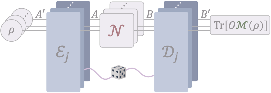
Figure 1: Shadow simulation of quantum channels. A sender (Alice) and a receiver (Bob) are connected through a quantum channel ${\cal N}$. The task is to enable Bob to estimate the expectation value ${\sf Tr}[O{\cal M}(\rho)]$ of an arbitrary observable $O$ on the output state ${\cal M}(\rho)$ produced by a target channel ${\cal M}$ when acting on an arbitrary input state $\rho$ of a system in Alice’s laboratory. To achieve this task, Alice and Bob can coordinate their operations ${\cal E}_{j}$ and ${\cal D}_{j}$ by sharing random bits.

Shadow simulation can be viewed as a generalization of the task of quantum channel simulation Kretschmann and Werner (2004); Berta et al. (2011); Bennett et al. (2014); Duan and Winter (2015); Leung and Matthews (2015a); Wang et al. (2018); Fang et al. (2019). The crucial difference is that shadow simulation does not aim at reproducing the output states of a target channel, but only their “shadow information” Zhao et al. (2023a); Aaronson (2018), i.e., the information about the expectation values of all possible observables. This generalization is useful for quantum information processing in the noisy intermediate-scale quantum (NISQ) era Preskill (2018), where classical post-processing of expectation values can be used to simulate larger quantum memories Bravyi et al. (2016); Peng et al. (2020); Mitarai and Fujii (2021); Piveteau and Sutter (2023), probe properties of quantum systems Buscemi et al. (2013); Huang et al. (2020); Elben et al. (2023), mitigate errors Li and Benjamin (2017); Temme et al. (2017); Piveteau et al. (2021); Lostaglio and Ciani (2021); Suzuki et al. (2022); Cai et al. (2022), and simulate unphysical operations Jiang et al. (2021); Regula et al. (2021); Zhao et al. (2023b).

Remarkably, we find that shadow simulation is not constrained by the limits of conventional channel simulation. For example, we show that one can perfectly shadow-simulate the transmission of an arbitrarily large number of qubits using only a single-qubit channel, a task that cannot be achieved in conventional channel simulation. In this example, the transmission of a larger number of qubits is simulated at the price of an increase of the number of samples needed to accurately estimate the expectation values. Quite surprisingly, we also find scenarios where shadow simulation achieves lower error than conventional channel simulation without any overhead in sampling cost, provided that Alice and Bob have access to no-signaling quantum resources. Overall, our results reveal that shared classical randomness and classical post-processing are valuable resources for quantum communication and other quantum technologies.

Framework: virtual supermaps.— In conventional quantum channel simulation, the aim is to simulate the action of a target channel ${\cal M}$ (with input $A^{\prime}$ and output $B^{\prime}$) by using an available channel ${\cal N}$ (with input $A$ and output $B$). To convert channel ${\cal N}$ into an approximation of channel ${\cal M}$, Alice and Bob perform encoding and decoding channels ${\cal E}$ and ${\cal D}$ in their local laboratories, respectively, thus obtaining the new channel ${\cal D}\circ{\cal N}\circ{\cal E}$. In shadow simulation, instead, Bob can sample his decoding operation ${\cal D}$ from a set of channels $\{{\cal D}_{j}\}$ and, after the output has been measured, he can post-process the measurement statistics, taking arbitrary linear combinations of the outcome probabilities. In this way, Bob can effectively implement a linear map of the form $\widetilde{D}=\sum_{j}\,\lambda_{j}\,{\cal D}_{j}$, where $\{\lambda_{j}\}$ are arbitrary real numbers Buscemi et al. (2013); Temme et al. (2017); Jiang et al. (2021); Piveteau et al. (2022). Note that in general $\widetilde{\cal D}$ is not a valid quantum channel (completely positive, trace-preserving map), but rather a virtual channel, described by a Hermitian-preserving and trace-scaling map Zhao et al. (2023a); Yuan et al. (2023); Parzygnat et al. (2023); Yao et al. (2023); Chen et al. (2023).

More generally, Bob may share classical randomness with Alice, and coordinate his local operations with hers, as in Figure 1. Hence, Bob’s post-processing gives rise to linear maps of the form

$$\widetilde{\cal S}({\cal N})=\sum_{j}\lambda_{j}{\cal D}_{j}\circ{\cal N}\circ{\cal E}_{j}.$$ (1)

The linear map $\widetilde{\cal S}$ is an example of a supermap Chiribella et al. (2008, 2009, 2013), that is, a map acting on the vector space spanned by quantum operations. Unlike most supermaps considered so far, however, $\widetilde{\cal S}$ generally does not transform quantum channels into quantum channels due to the possible presence of negative coefficients in the set $\{\lambda_{j}\}$. Instead, $\widetilde{\cal S}$ transforms Hermitian-preserving maps into Hermitian-preserving maps, and trace-scaling maps into trace-scaling maps. We call the supermaps with these two properties virtual supermaps.

Any virtual supermap $\widetilde{\cal S}$ is into one-to-one correspondence with a virtual bipartite processes $\widehat{\cal S}$ transforming operators on system $A^{\prime}B$ into operators on system $AB^{\prime}$. The correspondence can be made explicit by decomposing the action of the virtual supermap $\widetilde{\cal S}$ as $\widetilde{\cal S}({\cal N})=\sum_{k}\,{\cal B}_{k}\circ{\cal N}\circ{\cal A}_{k}$, where ${\cal A}_{k}$ and ${\cal B}_{k}$ are suitable linear maps, and by defining $\widehat{\cal S}\coloneqq\sum_{k}{\cal A}_{k}\otimes{\cal B}_{k}$.

A virtual supermap $\widetilde{\cal S}$ of the special form (1) will be called a (randomness-assisted) shadow simulation code. For a shadow simulation code $\widetilde{\cal S}$, the corresponding virtual bipartite process is $\widehat{\cal S}\coloneqq\sum_{j}\,\lambda_{j}\,{\cal E}_{j}\otimes{\cal D}_{j}$. It is rather straightforward to see that this virtual process is no-signaling, meaning that for every pair of operators $\rho_{A^{\prime}}$ and $\rho_{B}$ acting on $A^{\prime}$ and $B$, respectively, the operator ${\sf Tr}_{B^{\prime}}[\widehat{\cal S}(\rho_{A^{\prime}}\otimes\rho_{B})]$ is independent of $\rho_{B}$, and the operator ${\sf Tr}_{A}[\widehat{\cal S}(\rho_{A^{\prime}}\otimes\rho_{B})]$ is independent of $\rho_{A^{\prime}}$. The converse is less straightforward but turns out to be true, yielding a complete characterization of the randomness-assisted shadow simulation codes:

Theorem 1

A virtual supermap $\widetilde{\cal S}$ is a randomness-assisted shadow simulation code if and only if the corresponding virtual process $\widehat{\cal S}$ is no-signaling.

The proof is provided in the Appendix. An important consequence of Theorem 1 is that shared randomness and classical post-processing can be used to simulate arbitrary no-signaling resources. Explicitly, a no-signaling resource is represented by a quantum no-signaling channel $\widehat{\cal S}$ Piani et al. (2006); Chiribella (2012) with input $A^{\prime}B$ and output $AB^{\prime}$. Using the no-signaling channel $\widehat{\cal S}$, Alice and Bob can implement the corresponding supermap $\widetilde{\cal S}$, which can be implemented using only shared randomness and classical post-processing, as guaranteed by Theorem 1. The same conclusion applies to protocols using local operations and shared entanglement, which is a special case of no-signaling resources.

No-signaling assisted shadow simulation.— Quantum no-signaling resources have been extensively studied in quantum Shannon theory Leung and Matthews (2015b); Duan and Winter (2015); Fang et al. (2019). We now extend their study to the task of shadow simulation. While in channel simulation Alice and Bob have the assistance of a fixed no-signaling channel, in shadow simulation they can more generally sample over a set of no-signaling channels $\{\widehat{\cal S}_{j}\}$. Using classical post-processing, they can reproduce the virtual supermap $\widetilde{\cal S}\coloneqq\sum_{j}\,\lambda_{j}\,\widetilde{\cal S}_{j}$. We call this supermap a no-signaling shadow simulation code.

The randomization over different settings generally comes at the price of an increased sampling cost, meaning that more rounds of data collection are needed to estimate the desired expectation values Jiang et al. (2021); Regula et al. (2021); Zhao et al. (2023b). To quantify this price, we define the sampling cost of the code $\widetilde{S}$ as

$$c_{\rm smp}\left(\widetilde{{\cal S}}\right) \coloneqq\inf\Big{\{}p_{+}+p_{-}~{}\Big{|}~{}\widehat{{\cal S}}=p_{+}\widehat{{\cal S}}^{+}-p_{-}\widehat{{\cal S}}^{-};$$

$$\qquad\qquad\qquad p_{\pm}\in\mathbb{R}^{+};~{}\widehat{{\cal S}}^{\pm}\in{\rm CPTP}\cap{\rm NS}\Big{\}},$$

where ${\rm CPTP}$ and ${\rm NS}$ denote the set of completely positive, trace-preserving maps and the set of no-signaling virtual processes, respectively, and $\mathbb{R}^{+}$ is the set of non-negative real numbers. Note that every conventional channel simulation protocol has $c_{\rm smp}\left(\widetilde{{\cal S}}\right)=1$, since the map $\widehat{{\cal S}}$ is a no-signaling channel. More discussion on the sampling cost is provided in the Appendix.

To quantify the simulation error, we adopt the diamond-norm distance $\|\widetilde{\cal S}({\cal N})-{\cal M}\|_{\diamond}/2\eqqcolon p_{\rm err}(\widetilde{{\cal S}};{\cal N},{\cal M})$ Kitaev (1997). This error measure applies to conventional and shadow simulation, with the only difference that in the conventional scenario the no-signaling bipartite map $\widehat{\cal S}$ is completely positive and trace-preserving, while in the shadow simulation scenario $\widehat{S}$ can be any Hermitian-preserving and trace-scaling map.

The optimal quantum limits to the task of shadow simulation can be quantified by two parameters. One is the minimum error achievable with sampling cost bounded by $\gamma$:

$$\varepsilon^{*}_{\gamma,\rm NS}({\cal N},{\cal M})\coloneqq\inf_{\widehat{{\cal S}}\in{\rm NS}}\left\{p_{\rm err}\left(\widetilde{{\cal S}};{\cal N},{\cal M}\right)~{}\middle|~{}c_{\rm smp}\left(\widetilde{{\cal S}}\right)\leq\gamma\right\}\,.$$

The other is the minimum sampling cost needed to guarantee that the error is below a given error tolerance $\varepsilon$:

$$\gamma^{*}_{\varepsilon,\rm NS}\left({\cal N},{\cal M}\right)\coloneqq\inf_{\widehat{{\cal S}}\in{\rm NS}}\left\{c_{\rm smp}\left(\widetilde{{\cal S}}\right)~{}\middle|~{}p_{\rm err}\left(\widetilde{{\cal S}};{\cal N},{\cal M}\right)\leq\varepsilon\right\}.$$

Both quantities can be computed efficiently by semidefinite programs (SDPs) given in the Appendix. In the following, we illustrate the power of shadow simulation in three applications.

Shadow communication.— Quantum communication can be viewed as a special case of channel simulation: the simulation of an identity channel acting on a given number of qubits. Here we consider the zero-error scenario Shannon (1956); Cubitt et al. (2011); Duan and Winter (2015); Wang and Duan (2016a), corresponding to an exact simulation of the identity channel. We define a zero-error shadow communication code $\widetilde{{\cal S}}$ as a supermap satisfying the condition $p_{\rm err}\left(\widetilde{{\cal S}};{\cal N},{\operatorname{id}}_{d}\right)=0$, where ${\operatorname{id}}_{d}$ denotes the identity channel on a $d$-dimensional quantum system. Then, we define the one-shot zero-error shadow capacity assisted by no-signaling resources as

$$Q^{(1)}_{\gamma,\rm NS}({\cal N})\coloneqq\sup_{d,\widehat{{\cal S}}\in{\rm NS}} \Big{\{}\log_{2}d~{}\Big{|}~{}\widetilde{{\cal S}}({\cal N})={\operatorname{id}}_{d},~{}c_{\rm smp}\left(\widetilde{{\cal S}}\right)\leq\gamma\Big{\}},$$ (2)

where the dimension $d$ is optimized over positive integers. Here the term “one-shot” refers to the fact that the communication protocol only involves quantum operations on the inputs and outputs of a single use of channel ${\cal N}$.

In the Appendix, we provide an explicit SDP expression for the shadow capacity for every given $\gamma$. This expression extends the previously known expression for the one-shot zero-error quantum capacity assisted by no-signaling resources  Duan and Winter (2015); Wang and Duan (2016b), which can be retrieved in the special case $\gamma=1$.

For $\gamma>1$, we show that the zero-error shadow capacity is generally larger than the zero-error quantum capacity. A concrete example is provided by the following theorem:

Theorem 2

Let ${\cal N}_{{\rm depo},p}(\rho)=p\rho+(1-p)\mathbbm{1}_{2}/2$ be a single-qubit depolarizing channel, where $p\in[0,1]$ is a probability and $\mathbbm{1}_{2}$ is the identity operator on $\mathbb{C}^{2}$. For $\gamma\geq 1$, the one-shot zero-error shadow capacity assisted by no-signaling resources is

$$Q^{(1)}_{\gamma,\rm NS}({\cal N}_{{\rm depo},p})=\log_{2}\left\lfloor\sqrt{2p\gamma+p+1}\right\rfloor.$$ (3)

Eq. (3) shows that the shadow capacity can become arbitrarily large as $\gamma$ grows, provided that the channel is not completely depolarizing ($p\neq 0$). In other words, a qubit depolarizing channel can be used to transmit the expectation values of all observables on a quantum system of arbitrarily high dimension, at the price of an increased sampling cost.

It is useful to compare the above finding with the existing results about error mitigation. Error mitigation protocols, such as those in Refs. Takagi (2021); Jiang et al. (2021), can be used to transmit arbitrary expectation values on a single-qubit state through repeated uses of a single-qubit depolarizing channel. This fact is interesting because, for $p\leq 1/3$, the depolarizing channel is entanglement-breaking Horodecki et al. (2003) and therefore it cannot reliably transmit quantum states, even if infinitely many copies of it are available. Theorem 2 takes this observation to a much stronger level: not only can a qubit depolarizing channel transmit all expectation values for a single qubit, but also it can transmit the expectation values on arbitrarily high-dimensional quantum systems.

Now, recall that Theorem 1 guarantees that every no-signaling code can be simulated with local operations and shared classical randomness, generally at the expense of a larger sampling cost. Combining this fact with Theorem 2, we obtain that randomness-assisted shadow simulation codes can have arbitrarily large capacity for sufficiently large values of the sampling cost. The same argument applies to shadow simulation codes assisted by shared entanglement. Remarkably, these phenomena are not limited to the depolarizing channel, but apply in general to every quantum channel achieving at least one non-zero value of the zero-error no-signaling assisted shadow capacity (2). The proof of this fact will be provided at the end of the next section.

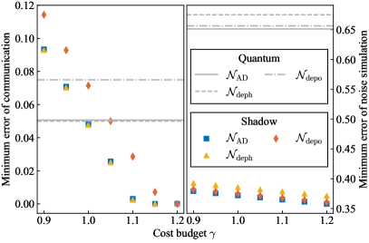
Figure 2: Minimum error of shadow simulation of common channels under different budgets for sampling cost. The channels we consider here are the amplitude damping channel, the dephasing channel, and the depolarizing channel at a low noise level ($p=0.9$). For communication (left), single-qubit versions of these channels are studied, and the goal is to simulate a qubit identity channel ${\operatorname{id}}_{2}$. For noise simulation (right), we consider simulating two-qubit versions of the noisy channels via ${\operatorname{id}}_{2}$, where by a two-qubit amplitude damping channel we mean two single-qubit amplitude damping channels acting independently on two qubits. Compared with that of conventional quantum channel simulation (gray lines), the minimum error in the shadow case is smaller with the same or even lower cost budget.

Shadow simulation via noiseless channels.— The dual task to communication is the simulation of a target noisy channel using a noiseless channel. In this case, the key quantity is the simulation cost, defined as the number of noiseless qubits that must be sent from the sender to a receiver. In the context of zero-error shadow simulation assisted by no-signaling resources, we define the one-shot shadow simulation cost of channel ${\cal M}$ as

$$S^{(1)}_{\gamma,\rm NS}({\cal M})\coloneqq\inf_{d,\widehat{{\cal S}}\in{\rm NS}} \Big{\{}\log_{2}d~{}\Big{|}~{}\widetilde{{\cal S}}({\operatorname{id}}_{d})={\cal M},~{}c_{\rm smp}\left(\widetilde{{\cal S}}\right)\leq\gamma\Big{\}},$$

where the dimension $d$ is optimized over positive integers. This quantity generalizes the one-shot zero-error simulation cost studied in the conventional quantum channel simulation scenario Duan and Winter (2015); Fang et al. (2019). In the Appendix, we provide an SDP for the zero-error shadow simulation cost, and we show that the simulation cost can generally be reduced by increasing the sampling cost.

Besides simulating noisy channels, shadow simulation also allows simulating high-dimensional noiseless channels using low-dimensional ones. This shadow simulation can also be viewed as a form of quantum compression, where the goal is to store the expectation values of all possible observables. Alternatively, one can view this shadow simulation as the simulation of a high-dimensional quantum measurement using a low-dimensional one. Differing from previous works that aimed at the simulation of the full measurement statistics Ioannou et al. (2022), however, shadow simulation focuses on the expectation values.

The minimum sampling cost for simulating a higher-dimensional identity channel is provided by the following theorem:

Theorem 3

Given identity channels ${\operatorname{id}}_{d}$ and ${\operatorname{id}}_{d^{\prime}}$ with $d^{\prime}\geq d\geq 2$, the minimum sampling cost of an exact shadow simulation of ${\operatorname{id}}_{d^{\prime}}$ using ${\operatorname{id}}_{d}$ and no-signaling resources is

$$\gamma^{*}_{0,\rm NS}\left({\operatorname{id}}_{d},{\operatorname{id}}_{d^{\prime}}\right)=2\left(\frac{d^{\prime}}{d}\right)^{2}-1.$$ (4)

Theorem 3 has two important implications. First, it implies that the shadow simulation cost of every quantum channel can be lowered to $1$ by allowing a sufficiently large sampling overhead. Indeed, let ${\cal M}$ be a quantum channel with one-shot zero-error quantum simulation cost $S^{(1)}_{\rm NS}({\cal M})=\log_{2}d^{\prime}$, meaning that ${\cal M}$ can be simulated using ${\operatorname{id}}_{d^{\prime}}$ through a quantum no-signaling code. In turn, Eq. (4) implies that ${\operatorname{id}}_{d^{\prime}}$ can be shadow-simulated using a qubit identity channel, with a sampling cost $(d^{\prime 2}-2)/2$. Composing the two simulations, one then gets a shadow simulation of ${\cal M}$ from ${\operatorname{id}}_{2}$ with sampling cost $(d^{\prime 2}-2)/2$.

Second, Theorem 3 implies that every channel ${\cal N}$ with non-zero shadow capacity $Q^{(1)}_{\gamma,\rm NS}$ for some $\gamma$ can shadow-simulate every other channel ${\cal M}$. In particular, it can simulate an identity channel on arbitrarily many qubits. This observation generalizes the result of Theorem 2 for single-qubit depolarizing channels.

Achieving lower error without sampling overhead.— In the zero-error scenario, we have seen that the shadow capacity and shadow simulation cost coincide with the conventional capacity and simulation cost for $\gamma=1$. In stark contrast, we now show that in the approximate scenario, shadow simulation can achieve lower error than conventional channel simulation even if $\gamma=1$, that is, without incurring a sampling overhead. As examples, we consider three common quantum channels: the single-qubit amplitude damping channel ${\cal N}_{\rm AD}$ with two Kraus operators $|0\rangle\!\langle 0|+\sqrt{p}|1\rangle\!\langle 1|$ and $\sqrt{1-p}|0\rangle\!\langle 1|$, the dephasing channel ${\cal N}_{\rm deph}(\cdot)=p(\cdot)+(1-p){\rm diag}(\cdot)$, and the depolarizing channel ${\cal N}_{\rm depo}(\cdot)=p(\cdot)+(1-p){\sf Tr}[\cdot]\mathbbm{1}_{d}/d$. For each channel, the parameter $p\in[0,1]$ indicates the level of the noise. For the depolarizing channel, the parameter $d$ represents the dimension of the system on which they act, and $\mathbbm{1}_{d}$ is the $d$-dimensional identity operator.

Figure 2 shows the minimum errors in both shadow communication and noisy channel simulation at different cost budgets ranging from $0.9$ to $1.2$. Surprisingly, shadow simulation codes achieve a smaller error at the same or even a lower level of cost compared with quantum simulation codes, whose sampling cost is $1$. The difference is more evident in the plot of noise simulation, where the minimum error of quantum codes is almost the twice of the shadow simulation codes. This implies that classical post-processing can enhance the transmission of expectation values even if no sampling overhead is involved.

Conclusions.— In this paper, we introduced the task of shadow simulation of quantum channels, showing that transmitting and processing expectation values of arbitrary observables is generally a less demanding task than transmitting and processing quantum states. Besides their foundational interest, our results are relevant to practical applications to NISQ quantum technologies, as they provide more efficient schemes for measuring observables at the output of noisy quantum devices. An interesting direction of future research is to explore scenarios where only a given set of physically relevant observables is concerned Aaronson (2018); Huang et al. (2020). Our results also open up a systematic way to study new quantum protocols that sample over different transformations of quantum processes, known as quantum supermaps Chiribella et al. (2008, 2009, 2013).

I Acknowledgments

We thank Yin Mo and Chengkai Zhu for useful comments that helped us improve the manuscript. This work has been supported by the Hong Kong Research Grant Council through grants 17307520 and R7035-21F, and by the John Templeton Foundation through grant 62312, The Quantum Information Structure of Spacetime (qiss.fr). The opinions expressed in this publication are those of the authors and do not necessarily reflect the views of the John Templeton Foundation. Research at the Perimeter Institute is supported by the Government of Canada through the Department of Innovation, Science and Economic Development Canada and by the Province of Ontario through the Ministry of Research, Innovation and Science. Xin Wang was supported by the Start-up Fund from The Hong Kong University of Science and Technology (Guangzhou), the Guangdong Quantum Science and Technology Strategic Fund (Grant No. GDZX2303007), and the Education Bureau of Guangzhou Municipality.

Appendix A Appendix A: Shadow Simulation Codes

A quantum simulation code $\left({\cal E}_{A^{\prime}\to A},{\cal D}_{B\to B^{\prime}}\right)$ can be written as a quantum supermap Chiribella et al. (2008), which sends a quantum channel ${\cal N}_{A\to B}$ to another quantum channel ${\cal M}_{A^{\prime}\to B^{\prime}}$. Each quantum supermap is associated with a bipartite quantum operation that is no-signaling from Bob to Alice, i.e., no transmission of information from Bob to Alice. In the setting of shadow simulation of quantum channels, simulation codes are not restricted to quantum supermaps. A shadow simulation code allows classical post-processing so that its encoding and decoding parts do not have to be quantum channels. For example, one can consider the encoding operation $\widetilde{{\cal E}}_{A^{\prime}\to A}\coloneqq\sum_{j}\lambda_{j}{\cal E}_{j,A^{\prime}\to A}$ and the decoding operation $\widetilde{{\cal D}}_{B\to B^{\prime}}\coloneqq\sum_{k}\mu_{k}{\cal D}_{k,B\to B^{\prime}}$ with real coefficients $\lambda_{j},\mu_{k}$ and quantum channels ${\cal E}_{j,A^{\prime}\to A},{\cal D}_{k,B\to B^{\prime}}$. The expectation value with respect to the state transmitted through a quantum channel ${\cal N}_{A\to B}$ using this shadow simulation code $\left(\widetilde{{\cal E}}_{A^{\prime}\to A},\widetilde{{\cal D}}_{B\to B^{\prime}}\right)$ can be decomposed as

$${\sf Tr}\left[\widetilde{{\cal D}}_{B\to B^{\prime}}\circ{\cal N}_{A\to B}\circ\widetilde{{\cal E}}_{A^{\prime}\to A}(\rho_{A})O_{B^{\prime}}\right]=\sum_{j,k}\lambda_{j}\mu_{k}{\sf Tr}\left[{\cal D}_{k,B\to B^{\prime}}\circ{\cal N}_{A\to B}\circ{\cal E}_{j,A^{\prime}\to A}(\rho_{A^{\prime}})O_{B^{\prime}}\right].$$ (A1)

Hence, although we cannot directly implement $\widetilde{{\cal E}}_{A^{\prime}\to A}$ and $\widetilde{{\cal D}}_{B\to B^{\prime}}$, we can simulate their effect by sending copies of the state using quantum simulation codes sampled from $\left\{\left({\cal E}_{j,A^{\prime}\to A},{\cal D}_{k,B\to B^{\prime}}\right)\right\}$ for multiple rounds and then post-processing the measurement results from all rounds.

Though the encoding operation $\widetilde{{\cal E}}$ and the decoding operation $\widetilde{{\cal D}}$ are seemingly independent, it is important to note that both maps are implemented with classical post-processing, which only happens at Bob’s side after Bob completes the measurement. Therefore, Bob needs information on Alice’s sampled operation in each round to guide the post-processing. Hence, we consider simulation codes where Alice and Bob have pre-shared randomness, and such codes are realized by the following steps:

1. Alice randomly samples one encoding channel ${\cal E}_{\alpha,A^{\prime}\to A}$ from the set of channels $\left\{{\cal E}_{j,A^{\prime}\to A}\right\}$ with a probability distribution $\Pr\left({\cal E}_{j,A^{\prime}\to A}\right)=|\lambda_{j}|/\gamma$, where $\gamma=\sum_{j}|\lambda_{j}|$, and applies the sampled channel to state $\rho_{A^{\prime}}$.

2. Alice then sends the post-encoding state ${\cal E}_{\alpha,A^{\prime}\to A}(\rho_{A^{\prime}})$ into the noisy channel ${\cal N}_{A\to B}$.

3. Upon receiving the state ${\cal N}_{A\to B}\circ{\cal E}_{\alpha,A^{\prime}\to A}(\rho_{A^{\prime}})$ coming out of the noisy channel, Bob applies the decoding channel ${\cal D}_{\alpha,B\to B^{\prime}}$ to the received state, where the value $\alpha$ is known to Bob due to the classical randomness shared between him and Alice.

4. Bob measures the decoded state ${\cal D}_{\alpha,B\to B^{\prime}}\circ{\cal N}_{A\to B}\circ{\cal E}_{\alpha,A^{\prime}\to A}(\rho_{A^{\prime}})$ with an observable $O_{B^{\prime}}$, which gives a measurement outcome $o$.

5. Repeat the above steps for $M$ times, and denote the index $\alpha$ and the measurement outcome $o$ in the $m$-th round by $\alpha_{m}$ and $o_{m}$, respectively. Then, compute $\xi\coloneqq\frac{\gamma}{M}\sum_{m=1}^{M}{\rm sgn}(\lambda_{\alpha_{m}})o_{m}$ as the communicated expectation value, where ${\rm sgn}$ is the sign function.

This protocol offers an unbiased estimator $\xi$ for the desired expectation value ${\sf Tr}\left[\left(\widetilde{{\cal S}}\left({\cal N}\right)\right)(\rho)O\right]$, where $\widetilde{{\cal S}}$ is a virtual supermap representing a randomness-assisted shadow simulation code whose action on ${\cal N}_{A\to B}$ is

$$\widetilde{\cal S}({\cal N})_{A^{\prime}\to B^{\prime}}=\sum_{j}\lambda_{j}{\cal D}_{j,B\to B^{\prime}}\circ{\cal N}_{A\to B}\circ{\cal E}_{j,A^{\prime}\to A}.$$ (A2)

This can be seen by checking the expectation value of $\xi$:

$$\mathbb{E}\left[\xi\right] =\frac{\gamma}{M}\sum_{m=1}^{M}\mathbb{E}\left[{\rm sgn}(\lambda_{\alpha_{m}})o_{m}\right]$$ (A3)

$$=\frac{\gamma}{M}\sum_{m=1}^{M}\sum_{j}\frac{\left|\lambda_{j}\right|}{\gamma}{\rm sgn}(\lambda_{j}){\sf Tr}\left[{\cal D}_{j}\circ{\cal N}\circ{\cal E}_{j}(\rho)O\right]$$ (A4)

$$=\frac{1}{M}\sum_{m=1}^{M}\sum_{j}\lambda_{j}{\sf Tr}\left[{\cal D}_{j}\circ{\cal N}\circ{\cal E}_{j}(\rho)O\right]$$ (A5)

$$={\sf Tr}\left[\sum_{j}\lambda_{j}{\cal D}_{j}\circ{\cal N}\circ{\cal E}_{j}(\rho)O\right]$$ (A6)

$$={\sf Tr}\left[\left(\widetilde{\cal S}({\cal N})\right)(\rho)O\right].$$ (A7)

Each supermap is associated with a bipartite map, and for a randomness-assisted shadow simulation code in Eq. (A2), its corresponding bipartite map is

$$\widehat{{\cal S}}_{A^{\prime}B\to AB^{\prime}}=\sum_{j}\lambda_{j}{\cal E}_{j,A^{\prime}\to A}\otimes{\cal D}_{j,B\to B^{\prime}}.$$ (A8)

It is clear that every randomness-assisted shadow simulation code is associated with a Hermitian-preserving bipartite map. This is because the Choi operator of the associated bipartite map is Hermitian, and a map is Hermitian-preserving if and only if its Choi operator is Hermitian. In the following, we show that bipartite maps associated with randomness-assisted shadow simulation codes, besides being Hermitian-preserving, are also no-signaling. For a bipartite map $\widehat{\cal S}_{A^{\prime}B\to AB^{\prime}}$, being no-signaling from Bob to Alice means that the output state at $A$ is independent of the input state at $B$, i.e., ${\sf Tr}_{B^{\prime}}\circ\widehat{\cal S}_{A^{\prime}B\to AB^{\prime}}=\widehat{\cal S}_{A^{\prime}\to A}\circ{\sf Tr}_{B}$, where $\widehat{\cal S}_{A^{\prime}\to A}$ is the local effective operation of the map $\widehat{\cal S}_{A^{\prime}B\to AB^{\prime}}$ from $A$ to $A^{\prime}$. By the Choi-Jamiołkowski isomorphism Jamiołkowski (1972); Choi (1975), we can uniquely represent $\widehat{\cal S}_{A^{\prime}B\to AB^{\prime}}$ using its Choi operator $J^{\widehat{\cal S}}_{A^{\prime}BAB^{\prime}}\coloneqq{\operatorname{id}}_{A^{\prime}B}\otimes\widehat{\cal S}_{\bar{A^{\prime}}\bar{B}\to AB^{\prime}}(|\Gamma\rangle\!\langle\Gamma|_{A^{\prime}B\bar{A^{\prime}}\bar{B}})$, where $|\Gamma\rangle_{A^{\prime}B\bar{A^{\prime}}\bar{B}}\coloneqq\sum_{j=0}^{d_{A^{\prime}B}-1}|j\rangle_{A^{\prime}B}|j\rangle_{\bar{A^{\prime}}\bar{B}}$ is the unnormalized maximally entangled state, $d_{A^{\prime}B}$ is the dimension of the system $A^{\prime}B$, and the Hilbert space associated with the system $\bar{A^{\prime}}\bar{B}$ is isomorphic to that of $A^{\prime}B$. In terms of the map’s Choi operator, no-signaling from Bob to Alice means ${\sf Tr}_{B^{\prime}}\left[J^{\widehat{\cal S}}_{A^{\prime}BAB^{\prime}}\right]=J^{\widehat{\cal S}}_{A^{\prime}A}\otimes\mathbbm{1}_{B}$, where $J^{\widehat{\cal S}}_{A^{\prime}A}\coloneqq{\sf Tr}_{BB^{\prime}}[J^{\widehat{\cal S}}_{A^{\prime}BAB^{\prime}}]/d_{B}$.

Theorem 1 shows that randomness-assisted shadow simulation codes are equivalent to Hermitian-preserving no-signaling bipartite maps, which is both no-signaling from Bob to Alice and no-signaling from Alice to Bob.

Theorem 1

A virtual supermap $\widetilde{\cal S}$ is a randomness-assisted shadow simulation code if and only if the corresponding virtual process $\widehat{\cal S}$ is no-signaling.

Proof.

For the “only if” part, let $\widehat{\cal S}_{A^{\prime}B\to AB^{\prime}}=\sum_{j}\lambda_{j}{\cal M}^{(j)}_{A^{\prime}\to A}\otimes{\cal N}^{(j)}_{B\to B^{\prime}}$ denote a bipartite map associated with an arbitrary randomness-assisted code, where ${\cal M}^{(j)}_{A^{\prime}\to A}$ and ${\cal N}^{(j)}_{B\to B^{\prime}}$ are quantum channels. It is clear that the Choi operator $J^{\widehat{\cal S}}_{A^{\prime}BAB^{\prime}}=\sum_{j}\lambda_{j}J^{{\cal M}^{(j)}}_{A^{\prime}A}\otimes J^{{\cal N}^{(j)}}_{BB^{\prime}}$ is Hermitian, indicating that $\widehat{\cal S}_{A^{\prime}B\to AB^{\prime}}$ is Hermitian-preserving. Furthermore, as ${\cal M}^{(j)}_{A^{\prime}\to A}$ and ${\cal N}^{(j)}_{B\to B^{\prime}}$ are trace-preserving, i.e., ${\sf Tr}_{A}\left[J^{{\cal M}^{(j)}}_{A^{\prime}A}\right]=\mathbbm{1}_{A^{\prime}}$ and ${\sf Tr}_{B^{\prime}}\left[J^{{\cal N}^{(j)}}_{BB^{\prime}}\right]=\mathbbm{1}_{B}$, we have

$${\sf Tr}_{A}\left[J^{\widehat{\cal S}}_{A^{\prime}BAB^{\prime}}\right] =\sum_{j}\lambda_{j}{\sf Tr}_{A}\left[J^{{\cal M}^{(j)}}_{A^{\prime}A}\right]\otimes J^{{\cal N}^{(j)}}_{BB^{\prime}}=\mathbbm{1}_{A^{\prime}}\otimes\sum_{j}\lambda_{j}J^{{\cal N}^{(j)}}_{BB^{\prime}}$$ (A9)

and

$${\sf Tr}_{B^{\prime}}\left[J^{\widehat{\cal S}}_{A^{\prime}BAB^{\prime}}\right] =\sum_{j}\lambda_{j}J^{{\cal M}^{(j)}}_{A^{\prime}A}\otimes{\sf Tr}_{B^{\prime}}\left[J^{{\cal N}^{(j)}}_{BB^{\prime}}\right]=\sum_{j}\lambda_{j}J^{{\cal M}^{(j)}}_{A^{\prime}A}\otimes\mathbbm{1}_{B},$$ (A10)

which imply that $\widehat{\cal S}_{A^{\prime}B\to AB^{\prime}}$ is no-signaling.

For the “if” part, we first assume that $\widehat{\cal S}_{A^{\prime}B\to AB^{\prime}}$ is Hermitian-preserving and no-signaling. By Theorem 14 in Ref. Gutoski (2009), its Choi operator can be decomposed as

$$J^{\widehat{\cal S}}_{A^{\prime}BAB^{\prime}}=\sum_{j}\lambda_{j}M^{(j)}_{A^{\prime}A}\otimes N^{(j)}_{BB^{\prime}},$$ (A11)

where, for each $j$, $\lambda_{j}$ is a real number, and $M^{(j)}_{A^{\prime}A}$ and $N^{(j)}_{BB^{\prime}}$ are Hermitian operators such that ${\sf Tr}_{A}\left[M^{(j)}_{A^{\prime}A}\right]$ and ${\sf Tr}_{B^{\prime}}\left[N^{(j)}_{BB^{\prime}}\right]$ are proportional to the identity operators $\mathbbm{1}_{A^{\prime}}$ and $\mathbbm{1}_{B}$, respectively. In other words, we can treat $M^{(j)}_{A^{\prime}A}$ and $N^{(j)}_{BB^{\prime}}$ as Choi operators for some Hermitian-preserving and trace-scaling (HPTS) maps $\widetilde{{\cal M}}^{(j)}_{A^{\prime}\to A}$ and $\widetilde{{\cal N}}^{(j)}_{B\to B^{\prime}}$, respectively. Here, trace-scaling means that the map scales the trace of the input operator with a constant factor.

According to Lemma 6 in Ref. Zhao et al. (2023a), every HPTS map can be written as a linear combination of two quantum channels. Thus, we can write $\widehat{\cal S}_{A^{\prime}B\to AB^{\prime}}$ as

$$\widehat{\cal S}_{A^{\prime}B\to AB^{\prime}} =\sum_{j}\lambda_{j}\widetilde{{\cal M}}^{(j)}_{A^{\prime}\to A}\otimes\widetilde{{\cal N}}^{(j)}_{B\to B^{\prime}}$$ (A12)

$$=\sum_{j}\lambda_{j}\left(m_{1}{\cal M}^{(j,1)}_{A^{\prime}\to A}+m_{2}{\cal M}^{(j,2)}_{A^{\prime}\to A}\right)\otimes\left(n_{1}{\cal N}^{(j,1)}_{B\to B^{\prime}}+n_{2}{\cal N}^{(j,2)}_{B\to B^{\prime}}\right)$$ (A13)

$$=\sum_{j}\sum_{k=1}^{2}\sum_{l=1}^{2}\lambda_{j}m_{k}n_{l}{\cal M}^{(j,k)}_{A^{\prime}\to A}\otimes{\cal N}^{(j,l)}_{B\to B^{\prime}},$$ (A14)

which represents a randomness-assisted shadow simulation code.     $\sqcap$$\sqcup$

Alternative to pre-shared classical randomness, forward classical communication from Alice to Bob also allows Bob to acquire information on Alice’s local operation in each round. A shadow simulation protocol with the assistance of forward classical communication is represented by a bipartite linear map

$$\widehat{{\cal S}}_{A^{\prime}B\to AB^{\prime}}=\sum_{j}\lambda_{j}{\cal M}^{(j)}_{A^{\prime}\to A}\otimes{\cal N}^{(j)}_{B\to B^{\prime}},$$ (A15)

where $\left\{{\cal M}^{(j)}_{A^{\prime}\to A}\right\}_{j}$ is a quantum instrument, $\left\{{\cal N}^{(j)}_{B\to B^{\prime}}\right\}_{j}$ is a collection of quantum channels, and each $\lambda_{j}$ is a real coefficient. In the following proposition, we show that not only $\widehat{{\cal S}}_{A^{\prime}B\to AB^{\prime}}$ is Hermitian-preserving and one-way no-signaling, but any one-way no-signaling Hermitian-preserving bipartite map represents a forward-classical-assisted shadow simulation code. For completeness, we also consider shadow simulation codes assisted by two-way classical communication, where both $\left\{{\cal M}^{(j)}_{A^{\prime}\to A}\right\}_{j}$ and $\left\{{\cal N}^{(j)}_{B\to B^{\prime}}\right\}_{j}$ are quantum instruments. Such codes are equivalent to the set of all bipartite Hermitian-preserving maps.

Theorem 4

Consider a bipartite linear map $\widehat{\cal S}_{A^{\prime}B\to AB^{\prime}}$. It is Hermitian-preserving if and only if it corresponds to a shadow simulation code assisted by two-way classical communication. It is Hermitian-preserving and $B$-to-$A$ no-signaling if and only if it corresponds to a forward-classical-assisted shadow simulation code.

This theorem tells us that shadow simulation codes with one-way classical communication are powerful enough to simulate arbitrary quantum channels and even beyond. An intuitive explanation is that Alice can measure the initial state $\rho$ with an informationally complete POVM and communicate the measurement outcomes to Bob so that Bob is able to reconstruct the expectation value of every observable on $\rho$ transformed by any channel. Now, we prove this theorem by proving the following two lemmas.

Lemma 5

A bipartite linear map $\widehat{\cal S}_{A^{\prime}B\to AB^{\prime}}$ is Hermitian-preserving and $B$-to-$A$ no-signaling if and only if it corresponds to a forward-classical-assisted shadow simulation code.

Proof.

The “if” direction is straightforward. Let $\widehat{\cal S}_{A^{\prime}B\to AB^{\prime}}=\sum_{j}\lambda_{j}{\cal M}^{(j)}_{A^{\prime}\to A}\otimes{\cal N}^{(j)}_{B\to B^{\prime}}$ represent a forward-classical-assisted shadow simulation code, where each $\left\{{\cal M}^{(j)}_{A^{\prime}\to A}\right\}_{j}$ is a quantum instrument, and each ${\cal N}^{(j)}_{B\to B^{\prime}}$ is a quantum channel. Then, the Choi operator of $\widehat{\cal S}_{A^{\prime}B\to AB^{\prime}}$ is

$$J^{\widehat{\cal S}}_{A^{\prime}BAB^{\prime}}=\sum_{j}\lambda_{j}J^{{\cal M}^{(j)}}_{A^{\prime}A}\otimes J^{{\cal N}^{(j)}}_{BB^{\prime}}.$$ (A16)

Clearly, $J^{\widehat{\cal S}}_{A^{\prime}BAB^{\prime}}$ is a Hermitian operator, indicating that $\widehat{\cal S}_{A^{\prime}B\to AB^{\prime}}$ is Hermitian-preserving. In addition, $\widehat{\cal S}_{A^{\prime}B\to AB^{\prime}}$ is no-signaling from Bob to Alice as

$${\sf Tr}_{B^{\prime}}\left[J^{\widehat{\cal S}}_{A^{\prime}BAB^{\prime}}\right]=\sum_{j}\lambda_{j}J^{{\cal M}^{(j)}}_{A^{\prime}A}\otimes{\sf Tr}_{B^{\prime}}\left[J^{{\cal N}^{(j)}}_{BB^{\prime}}\right]=\sum_{j}\lambda_{j}J^{{\cal M}^{(j)}}_{A^{\prime}A}\otimes\mathbbm{1}_{B}$$ (A17)

due to ${\cal N}$ being trace-preserving.

For the “only if” direction, part of the proof is adapted from the proof of Theorem 14 in Ref. Gutoski (2009). Let $\widehat{\cal S}_{A^{\prime}B\to AB^{\prime}}$ be a Hermitian-preserving supermap and $\left\{M^{(1)}_{A^{\prime}A},\dots,M^{(D)}_{A^{\prime}A}\right\}$ be a basis for the Hermitian operator space ${\rm Herm}\left(A^{\prime}A\right)$ on the system $A^{\prime}A$, where $D$ is the dimension of this space. Then, there exists a unique set of Hermitian operators $\left\{N^{(1)}_{BB^{\prime}},\dots,N^{(D)}_{BB^{\prime}}\right\}\subseteq{\rm Herm}\left(BB^{\prime}\right)$ such that $J^{\widehat{\cal S}}_{A^{\prime}BAB^{\prime}}=\sum_{j=1}^{D}M^{(j)}_{A^{\prime}A}\otimes N^{(j)}_{BB^{\prime}}$. For each $j$, let $H^{(j)}_{A^{\prime}A}$ be a Hermitian operator such that ${\sf Tr}\left[H^{(j)}_{A^{\prime}A}M^{(k)}_{A^{\prime}A}\right]\neq 0$ if and only if $j=k$. Denoting the mapping $M_{A^{\prime}A}\mapsto{\sf Tr}\left[H^{(j)}_{A^{\prime}A}M^{(k)}_{A^{\prime}A}\right]$ by $h^{(j)}(M_{A^{\prime}A})$, we have

$$\left(h^{(j)}\otimes{\operatorname{id}}_{BB^{\prime}}\right)\left(J^{\widehat{\cal S}}_{A^{\prime}BAB^{\prime}}\right)=\sum_{k=1}^{D}h^{(j)}\left(M^{(k)}_{A^{\prime}A}\right)\otimes N^{(k)}_{BB^{\prime}}=h^{(j)}\left(M^{(j)}_{A^{\prime}A}\right)N^{(j)}_{BB^{\prime}}.$$ (A18)

Because $\widehat{\cal S}_{A^{\prime}B\to AB^{\prime}}$ is no-signaling from Bob to Alice, we have ${\sf Tr}_{B^{\prime}}\left[J^{\widehat{\cal S}}_{A^{\prime}BAB^{\prime}}\right]=J^{\widehat{\cal S}}_{A^{\prime}A}\otimes\mathbbm{1}_{B}$. Then,

$$\left(h^{(j)}\otimes{\operatorname{id}}_{BB^{\prime}}\right){\sf Tr}_{B^{\prime}}\left[J^{\widehat{\cal S}}_{A^{\prime}BAB^{\prime}}\right]=h^{(j)}\left(J^{\widehat{\cal S}}_{A^{\prime}A}\right)\otimes\mathbbm{1}_{B}=h^{(j)}\left(M^{(j)}_{A^{\prime}A}\right){\sf Tr}_{B^{\prime}}\left[N^{(j)}_{BB^{\prime}}\right],$$ (A19)

where the second equality holds because the order of applying $\left(h^{(j)}\otimes{\operatorname{id}}_{BB^{\prime}}\right)$ and ${\sf Tr}_{B^{\prime}}$ does not affect the result as they act on different subspaces.

It follows from Eq. (A19) that, for each $j$, ${\sf Tr}_{B^{\prime}}\left[N^{(j)}_{BB^{\prime}}\right]$ is proportional to the identity operator $\mathbbm{1}_{B}$, and thus it serves as a Choi operator of an HPTS map, which we denote by $\widetilde{{\cal N}}^{(j)}_{B\to B^{\prime}}$. According to Lemma 6 in Ref. Zhao et al. (2023a), each $\widetilde{{\cal N}}^{(j)}_{B\to B^{\prime}}$ can be written as a linear combination of two quantum channels, i.e.,

$$\widetilde{{\cal N}}^{(j)}_{B\to B^{\prime}}=n_{j,1}{\cal N}^{(j,1)}_{B\to B^{\prime}}+n_{j,2}{\cal N}^{(j,2)}_{B\to B^{\prime}},$$ (A20)

where $n_{j,1}$ and $n_{j,2}$ are real numbers and ${\cal N}^{(j,1)}_{B\to B^{\prime}}$ and ${\cal N}^{(j,2)}_{B\to B^{\prime}}$ are quantum channels.

For each Hermitian operator $M^{(j)}_{A^{\prime}A}$, we can write it as the difference of two positive semidefinite operators, say, $m_{j,1}M^{(j,1)}_{A^{\prime}A}-m_{j,2}M^{(j,2)}_{A^{\prime}A}$, where $m_{j,1}M^{(j,1)}_{A^{\prime}A}$ and $m_{j,2}M^{(j,2)}_{A^{\prime}A}$ are positive semidefinite and $m_{j,1}$ and $m_{j,2}$ are positive real numbers so that ${\sf Tr}_{A}\left[M^{(j,1)}_{A^{\prime}A}\right]\leq\mathbbm{1}_{A^{\prime}}$ and ${\sf Tr}_{A}\left[M^{(j,2)}_{A^{\prime}A}\right]\leq\mathbbm{1}_{A^{\prime}}$. In other words, both $M^{(j,1)}_{A^{\prime}A}$ and $M^{(j,2)}_{A^{\prime}A}$ are Choi operators of some completely positive and trace-non-increasing (CPTN) maps, say ${\cal M}^{(j,1)}_{A^{\prime}\to A}$ and ${\cal M}^{(j,2)}_{A^{\prime}\to A}$, respectively. Moreover, the scalars $m_{j,1}$ and $m_{j,2}$ should be chosen so that $\sum_{j=1}^{D}\sum_{k=1}^{2}{\sf Tr}_{A}\left[M^{(j,k)}_{A^{\prime}A}\right]\leq\mathbbm{1}_{A^{\prime}}/2$. We will see the reason of this requirement later.

Combining the decomposition of every $M^{(j)}_{A^{\prime}A}$ and every $N^{(j)}_{BB^{\prime}}$, we have

$${\cal S}_{A^{\prime}B\to AB^{\prime}} =\sum_{j=1}^{D}\left(m_{j,1}{\cal M}^{(j,1)}_{A^{\prime}\to A}-m_{j,2}{\cal M}^{(j,2)}_{A^{\prime}\to A}\right)\otimes\left(n_{j,1}{\cal N}^{(j,1)}_{B\to B^{\prime}}+n_{j,2}{\cal N}^{(j,2)}_{B\to B^{\prime}}\right)$$ (A21)

$$=\sum_{j=1}^{D}\Big{(}m_{j,1}n_{j,1}{\cal M}^{(j,1)}_{A^{\prime}\to A}\otimes{\cal N}^{(j,1)}_{B\to B^{\prime}}+m_{j,1}n_{j,2}{\cal M}^{(j,1)}_{A^{\prime}\to A}\otimes{\cal N}^{(j,2)}_{B\to B^{\prime}}$$

$$\qquad-m_{j,2}n_{j,1}{\cal M}^{(j,2)}_{A^{\prime}\to A}\otimes{\cal N}^{(j,1)}_{B\to B^{\prime}}-m_{j,2}n_{j,2}{\cal M}^{(j,2)}_{A^{\prime}\to A}\otimes{\cal N}^{(j,2)}_{B\to B^{\prime}}\Big{)}$$ (A22)

$$=\sum_{j=1}^{4D}\lambda_{j}{\cal M}^{(j)}_{A^{\prime}\to A}\otimes{\cal N}^{(j)}_{B\to B^{\prime}}$$ (A23)

with appropriate relabeling, where each $\lambda_{j}\in\left\{m_{j,1}n_{j,1},m_{j,1}n_{j,2},-m_{j,2}n_{j,1},-m_{j,2}n_{j,2}\right\}_{j}$ is a real number, each ${\cal M}^{(j)}_{A^{\prime}\to A}\in\left\{{\cal M}^{(j,1)}_{A^{\prime}\to A},{\cal M}^{(j,2)}_{A^{\prime}\to A}\right\}_{j}$ is a CPTN map, and each ${\cal N}^{(j)}_{B\to B^{\prime}}\in\left\{{\cal N}^{(j,1)}_{B\to B^{\prime}},{\cal N}^{(j,2)}_{B\to B^{\prime}}\right\}_{j}$ is a quantum channel. Note that

$$\sum_{j=1}^{4D}{\sf Tr}_{A}\left[J^{{\cal M}^{(j)}}_{A^{\prime}A}\right]=2\sum_{j=1}^{D}\sum_{k=1}^{2}{\sf Tr}_{A}\left[J^{{\cal M}^{(j,k)}}_{A^{\prime}A}\right]\leq\mathbbm{1}_{A^{\prime}}$$ (A24)

due to our choice of scalars $\left\{m_{j,1},m_{j,2}\right\}_{j}$. Let ${\cal M}^{\prime}_{A^{\prime}\to A}$ be a CPTN map such that $\sum_{j=1}^{4D}{\sf Tr}_{A}\left[J^{{\cal M}^{(j)}}_{A^{\prime}A}\right]+2{\sf Tr}_{A}\left[J^{{\cal M}^{\prime}}_{A^{\prime}A}\right]=\mathbbm{1}_{A^{\prime}}$. Then, $\left\{{\cal M}^{(1)},\dots,{\cal M}^{(4D)},{\cal M}^{\prime},{\cal M}^{\prime}\right\}$ is a quantum instrument and

$$\widehat{\cal S}_{A^{\prime}B\to AB^{\prime}}=\sum_{j=1}^{4D}\lambda_{j}{\cal M}^{(j)}_{A^{\prime}\to A}\otimes{\cal N}^{(j)}_{B\to B^{\prime}}+{\cal M}^{\prime}_{A^{\prime}\to A}\otimes{\cal N}^{\prime}_{B\to B^{\prime}}-{\cal M}^{\prime}_{A^{\prime}\to A}\otimes{\cal N}^{\prime}_{B\to B^{\prime}}$$ (A25)

for any quantum channel ${\cal N}^{\prime}_{B\to B^{\prime}}$. Therefore, any bipartite linear map ${\cal S}_{A^{\prime}B\to AB^{\prime}}$ that is Hermitian-preserving and $B$-to-$A$ no-signaling represents a forward-classical-assisted shadow simulation code.     $\sqcap$$\sqcup$

Lemma 6

A bipartite linear map $\widehat{\cal S}_{A^{\prime}B\to AB^{\prime}}$ is Hermitian-preserving if and only if it corresponds to a shadow simulation code assisted by two-way classical communication.

Proof.

The “if” part can be directly verified by checking that the Choi operator of a bipartite map $\sum_{j}\lambda_{j}{\cal M}^{(j)}_{A^{\prime}\to A}\otimes{\cal N}^{(j)}_{B\to B^{\prime}}$ is Hermitian, where both $\left\{{\cal M}^{(j)}_{A^{\prime}\to A}\right\}_{j}$ and $\left\{{\cal N}^{(j)}_{B\to B^{\prime}}\right\}_{j}$ are quantum instruments.

For the “only if” part, we follow the proof of Lemma 5 to write the Choi operator of a bipartite Hermitian-preserving map $\widehat{\cal S}_{A^{\prime}B\to AB^{\prime}}$ as $J^{\widehat{\cal S}}_{A^{\prime}BAB^{\prime}}=\sum_{j=1}^{D}M^{(j)}_{A^{\prime}A}\otimes N^{(j)}_{BB^{\prime}}$, where $M^{(j)}_{A^{\prime}A}$ and $N^{(j)}_{BB^{\prime}}$ are Hermitian operators. Each $M^{(j)}_{A^{\prime}A}$ or $N^{(j)}_{BB^{\prime}}$ can be written as the difference of two positive semidefinite operators. We write each $M^{(j)}_{A^{\prime}A}$ as $m_{j,+}M^{(j,+)}_{A^{\prime}A}-m_{j,-}M^{(j,-)}_{A^{\prime}A}$ and each $N^{(j)}_{BB^{\prime}}$ as $n_{j,+}N^{(j,+)}_{BB^{\prime}}-n_{j,-}N^{(j,-)}_{BB^{\prime}}$, where $m_{j,\pm}M^{(j,1)}_{A^{\prime}A},n_{j,2}N^{(j,\pm)}_{BB^{\prime}}$ are positive semidefinite and $m_{j,\pm},n_{j,\pm}$ are positive real numbers that will be fixed later. The Choi operator $J^{\widehat{\cal S}}_{A^{\prime}BAB^{\prime}}$ now can be written as

$$J^{\widehat{\cal S}}_{A^{\prime}BAB^{\prime}} =\sum_{j=1}^{D}\left(m_{j,+}M^{(j,+)}_{A^{\prime}A}-m_{j,-}M^{(j,-)}_{A^{\prime}A}\right)\otimes\left(n_{j,+}N^{(j,+)}_{BB^{\prime}}-n_{j,-}N^{(j,-)}_{BB^{\prime}}\right)$$ (A26)

$$=\sum_{j=1}^{D}\sum_{k\in\left\{+,-\right\}}\sum_{l\in\left\{+,-\right\}}(-1)^{1-\delta_{k,l}}m_{j,k}n_{j,l}M^{(j,k)}_{A^{\prime}A}\otimes N^{(j,l)}_{BB^{\prime}},$$ (A27)

where $\delta_{k,l}=1$ if $k=l$ and $\delta_{k,l}=0$ otherwise. Because $M^{(j,\pm)}_{A^{\prime}A}$ and $N^{(j,\pm)}_{BB^{\prime}}$ are positive semidefinite operators, they can be treated as Choi operators of completely positive maps, say, ${\cal M}^{(j,\pm)}_{A^{\prime}\to A}$ and ${\cal N}^{(j,\pm)}_{B\to B^{\prime}}$. Then, we can write $\widehat{\cal S}_{A^{\prime}B\to AB^{\prime}}$ as

$$\widehat{\cal S}_{A^{\prime}B\to AB^{\prime}} =\sum_{j=1}^{D}\sum_{k\in\left\{+,-\right\}}\sum_{l\in\left\{+,-\right\}}(-1)^{1-\delta_{k,l}}m_{j,k}n_{j,l}{\cal M}^{(j,k)}_{A^{\prime}\to A}\otimes{\cal N}^{(j,l)}_{B\to B^{\prime}}$$ (A28)

$$=\sum_{j=1}^{4D}\lambda_{j}{\cal M}^{(j)}_{A^{\prime}\to A}\otimes{\cal N}^{(j)}_{B\to B^{\prime}}$$ (A29)

with appropriate relabeling, where each $\lambda_{j}\in\left\{(-1)^{1-\delta_{k,l}}m_{j,k}n_{j,l}\right\}_{j,k,l}$ is a real number, each ${\cal M}^{(j)}_{A^{\prime}\to A}\in\left\{{\cal M}^{(j,\pm)}_{A^{\prime}\to A}\right\}_{j}$ or ${\cal N}^{(j)}_{B\to B^{\prime}}\in\left\{{\cal N}^{(j,\pm)}_{B\to B^{\prime}}\right\}_{j}$ is a CPTN map. We can fix the values of the coefficients $m_{j,\pm}$ and $n_{j,\pm}$ to be large enough so that both $\sum_{j=1}^{4D}{\cal M}^{(j)}_{A^{\prime}\to A}$ and $\sum_{j=1}^{4D}{\cal N}^{(j)}_{B\to B^{\prime}}$ are trace-non-increasing. Let ${\cal M}^{\prime}_{A^{\prime}\to A}$ and ${\cal N}^{\prime}_{B\to B^{\prime}}$ be CPTN maps such that $\sum_{j=1}^{4D}{\cal M}^{(j)}_{A^{\prime}\to A}+2{\cal M}^{\prime}_{A^{\prime}\to A}$ and $\sum_{j=1}^{4D}{\cal N}^{(j)}_{B\to B^{\prime}}+2{\cal N}^{\prime}_{B\to B^{\prime}}$ are CPTP. That is, $\left\{{\cal M}^{(1)},\dots,{\cal M}^{(4D)},{\cal M}^{\prime},{\cal M}^{\prime}\right\}$ and $\left\{{\cal N}^{(1)},\dots,{\cal N}^{(4D)},{\cal N}^{\prime},{\cal N}^{\prime}\right\}$ are quantum instruments. Because we can write

$$\widehat{\cal S}_{A^{\prime}B\to AB^{\prime}}=\sum_{j=1}^{4D}\lambda_{j}{\cal M}^{(j)}_{A^{\prime}\to A}\otimes{\cal N}^{(j)}_{B\to B^{\prime}}+{\cal M}^{\prime}_{A^{\prime}\to A}\otimes{\cal N}^{\prime}_{B\to B^{\prime}}-{\cal M}^{\prime}_{A^{\prime}\to A}\otimes{\cal N}^{\prime}_{B\to B^{\prime}},$$ (A30)

it follows that $\widehat{\cal S}_{A^{\prime}B\to AB^{\prime}}$ corresponds to a shadow simulation code assisted by two-way classical communication. Hence the proof.     $\sqcap$$\sqcup$

From now on, we focus on no-signaling shadow simulation codes. We consider implementing such codes by sampling quantum no-signaling codes. This is possible due to the following proposition.

Proposition 7

A bipartite linear map is Hermitian-preserving and no-signaling if and only if it is a linear combination of bipartite linear maps that correspond to quantum no-signaling codes.

Proof.

For the “if” direction, let $\widehat{{\cal S}}_{A^{\prime}B\to AB^{\prime}}=\sum_{j}{\cal S}^{(j)}_{A^{\prime}B\to AB^{\prime}}$ be a linear combination of bipartite linear maps that correspond to quantum no-signaling codes. The map $\widehat{{\cal S}}_{A^{\prime}B\to AB^{\prime}}$ is Hermitian-preserving because $J^{\widehat{{\cal S}}}_{A^{\prime}BAB^{\prime}}$, the Choi operator of $\widehat{{\cal S}}_{A^{\prime}B\to AB^{\prime}}$, is Hermitian. Also, $\widehat{{\cal S}}_{A^{\prime}B\to AB^{\prime}}$ is no-signaling from $B$ to $A$, because

$${\sf Tr}_{B^{\prime}}\left[J^{\widehat{{\cal S}}}_{A^{\prime}BAB^{\prime}}\right]=\sum_{j}\lambda_{j}{\sf Tr}_{B^{\prime}}\left[J^{{\cal S}^{(j)}}_{A^{\prime}BAB^{\prime}}\right]=\sum_{j}\lambda_{j}J^{{\cal S}^{(j)}}_{A^{\prime}A}\otimes\mathbbm{1}_{B}=J^{\widehat{{\cal S}}}_{A^{\prime}A}\otimes\mathbbm{1}_{B},$$ (A31)

where the second inequality follows from each ${\cal S}^{(j)}_{A^{\prime}B\to AB^{\prime}}$ being no-signaling. Similarly, $\widehat{{\cal S}}_{A^{\prime}B\to AB^{\prime}}$ is no-signaling from $A$ to $B$ as

$${\sf Tr}_{A}\left[J^{\widehat{{\cal S}}}_{A^{\prime}BAB^{\prime}}\right]=\sum_{j}\lambda_{j}{\sf Tr}_{A}\left[J^{{\cal S}^{(j)}}_{A^{\prime}BAB^{\prime}}\right]=\sum_{j}\lambda_{j}J^{{\cal S}^{(j)}}_{BB^{\prime}}\otimes\mathbbm{1}_{A^{\prime}}=J^{\widehat{{\cal S}}}_{BB^{\prime}}\otimes\mathbbm{1}_{A^{\prime}}.$$ (A32)

Therefore, the map $\widehat{{\cal S}}_{A^{\prime}B\to AB^{\prime}}$ is Hermitian-preserving and no-signaling.

For the “only if” part, let $\widetilde{{\cal S}}_{A^{\prime}B\to AB^{\prime}}$ be a Hermitian-preserving and no-signaling bipartite linear map. According to Theorem 1, $\widehat{{\cal S}}_{A^{\prime}B\to AB^{\prime}}$ can be decomposed as $\widehat{{\cal S}}_{A^{\prime}B\to AB^{\prime}}=\sum_{j}\lambda_{j}{\cal M}^{(j)}_{A^{\prime}\to A}\otimes{\cal N}^{(j)}_{B\to B^{\prime}}$ for some quantum channels ${\cal M}^{(j)}_{A^{\prime}\to A}$ and ${\cal N}^{(j)}_{B\to B^{\prime}}$. Note that each ${\cal S}^{(j)}_{A^{\prime}B\to AB^{\prime}}\coloneqq{\cal M}^{(j)}_{A^{\prime}\to A}\otimes{\cal N}^{(j)}_{B\to B^{\prime}}$ is a bipartite linear map corresponding to a quantum no-signaling code. Therefore, $\widehat{{\cal S}}_{A^{\prime}B\to AB^{\prime}}=\sum_{j}\lambda_{j}{\cal S}^{(j)}_{A^{\prime}B\to AB^{\prime}}$ is indeed a linear combination of bipartite linear maps corresponding to quantum no-signaling codes.     $\sqcap$$\sqcup$

By decomposing it into a few quantum no-signaling codes, we can implement any no-signaling shadow simulation code by sampling quantum no-signaling codes in a way similar to the protocol given earlier in this section for realizing randomness-assisted shadow simulation codes. The implementation of a no-signaling shadow simulation code incurs a cost quantifying how many sampling rounds are required. Such a cost can be derived from Hoeffding’s inequality. Let $\widetilde{{\cal S}}=\sum_{j}\lambda_{j}{\cal S}_{j}$ be a no-signaling shadow simulation code decomposed into a linear combination of quantum no-signaling codes $\left\{{\cal S}_{j}\right\}$ so that

$${\sf Tr}\left[\left(\widetilde{{\cal S}}\left({\cal N}\right)\right)(\rho)O\right]=\sum_{j}\lambda_{j}{\sf Tr}\left[\left({\cal S}_{j}\left({\cal N}\right)\right)(\rho)O\right]$$ (A33)

for any quantum state $\rho$ and any observable $O$. We assume that the observable is bounded as $\|O\|_{\infty}\leq 1$ so that each measurement outcome belongs to the interval $[-1,1]$. For post-processing, we multiply each measurement outcome by a factor of magnitude $\gamma\coloneqq\sum_{j}|\lambda_{j}|$, and the average of all the post-processed outcomes serves as an unbiased estimator $\xi$ for ${\sf Tr}\left[\left(\widetilde{{\cal S}}\left({\cal N}\right)\right)(\rho)O\right]$. According to Hoeffding’s inequality Hoeffding (1994), the probability that the estimator has an error larger than or equal to $\epsilon$ is bounded as

$$\Pr\left(\left|\xi-\mathbb{E}\left[\xi\right]\right|\geq\epsilon\right)\leq 2\exp\left(-\frac{M\epsilon^{2}}{2\gamma^{2}}\right),$$ (A34)

where $M$ is the number of sampling rounds. Hence, we can conclude that

$$M\geq\frac{2\gamma^{2}\log\frac{2}{\delta}}{\epsilon^{2}}$$ (A35)

rounds are enough for the final estimation to have an error smaller than $\epsilon$ with a probability no less than $1-\delta$.

The number of rounds $M$ is proportional to $\gamma^{2}$, where $\gamma$ is the sum of the absolute values of the coefficients in the decomposition of $\widetilde{{\cal S}}$. Considering that a no-signaling shadow simulation code $\widetilde{{\cal S}}$ can have many different decompositions, we define its sampling cost as the smallest possible $\gamma$ achieved by any feasible decomposition:

$$c_{\rm smp}\left(\widetilde{{\cal S}}\right)\coloneqq\inf\left\{\sum_{j}\left|\lambda_{j}\right|~{}\middle|~{}\widehat{\cal S}=\sum_{j}\lambda_{j}\widehat{\cal S}_{j};~{}\lambda_{j}\in\mathbb{R};~{}\widehat{\cal S}_{j}\in\rm{CPTP}\cap\rm{NS}\right\}.$$ (A36)

Note that all the quantum no-signaling channels in the decomposition whose corresponding coefficients have the same sign can be grouped into one single quantum no-signaling channel without changing the cost. Hence, it is sufficient to consider all combinations in the form of $\widehat{\cal S}=p_{+}\widehat{\cal S}^{+}-p_{-}\widehat{\cal S}^{-}$, where $p_{\pm}$ are non-negative coefficients and $\widehat{\cal S}^{\pm}$ are quantum no-signaling channels:

$$c_{\rm smp}\left(\widetilde{{\cal S}}\right)=\inf\left\{p_{+}+p_{-}~{}\middle|~{}\widehat{\cal S}=p_{+}\widehat{\cal S}^{+}-p_{-}\widehat{\cal S}^{-};~{}p_{\pm}\in\mathbb{R}^{+};\widehat{\cal S}_{j}\in\rm{CPTP}\cap\rm{NS}\right\}.$$ (A37)

Appendix B Appendix B: General SDPs for Minimum Error and Minimum Sampling Cost

We show that the minimum sampling cost and the minimum error of shadow simulation assisted by no-signaling codes can be formulated as SDPs. The minimum sampling cost can be formulated as

$$\gamma^{*}_{\varepsilon,\rm NS}({\cal N},{\cal M})=\inf \;p_{+}+p_{-}$$ (B1a)

s.t. $$\;\widehat{\cal S}=p_{+}\widehat{\cal S}^{+}-p_{-}\widehat{\cal S}^{-},$$ (B1b)

$$\;\frac{1}{2}\left\|{\cal M}_{A^{\prime}\to B^{\prime}}-\widetilde{{\cal S}}\left({\cal N}_{A\to B}\right)\right\|_{\diamond}\leq\varepsilon,$$ (B1c)

$$\;\widehat{\cal S}^{\pm}\in\rm{CPTP}\cap{\rm NS}.$$ (B1d)

This optimization problem can be modified to one for $\varepsilon^{*}_{\gamma,\rm NS}\left({\cal N},{\cal M}\right)$ by changing the optimization objective to $\varepsilon$ and adding the constraint $p_{+}+p_{-}\leq\gamma$. For a pair of quantum channels, i.e., CPTP maps, the diamond distance between them can be efficiently computed via a simple SDP Watrous (2009). For shadow simulation, however, the map $\widetilde{{\cal S}}\left({\cal N}\right)$ is HPTS, which is more general than CPTP. Here, we show how to adapt the SDP for the diamond distance between two quantum channels to compute the diamond distance between any two HPTS maps.

Let $\widetilde{{\cal N}}_{A\to B}=p_{+}{\cal N}^{+}_{A\to B}-p_{-}{\cal N}^{-}_{A\to B}$ and $\widetilde{{\cal M}}_{A\to B}=q_{+}{\cal M}^{+}_{A\to B}-q_{-}{\cal M}^{-}_{A\to B}$ be two HPTS maps, where $p_{\pm}$ and $q_{\pm}$ are non-negative real numbers, and ${\cal N}^{\pm}_{A\to B}$ and ${\cal M}^{\pm}_{A\to B}$ are quantum channels. By the definition of the diamond norm, the diamond distance between these two maps is

$$\frac{1}{2}\left\|\widetilde{{\cal N}}_{A\to B}-\widetilde{{\cal M}}_{A\to B}\right\|_{\diamond} =\sup_{\psi_{RA}}\frac{1}{2}\left\|\widetilde{{\cal N}}_{A\to B}(\psi_{RA})-\widetilde{{\cal M}}_{A\to B}(\psi_{RA})\right\|_{1}$$ (B2)

$$=\sup_{\psi_{RA}}\bigg{\{}\sup_{M\mathrel{\mathop{\mathchar 58\relax}}0\leq M\leq\mathbbm{1}}{\sf Tr}\left[M\left(\widetilde{{\cal N}}_{A\to B}(\psi_{RA})-\widetilde{{\cal M}}_{A\to B}(\psi_{RA})\right)\right]$$

$$\qquad-\frac{1}{2}{\sf Tr}\left[\widetilde{{\cal N}}_{A\to B}(\psi_{RA})-\widetilde{{\cal M}}_{A\to B}(\psi_{RA})\right]\bigg{\}},$$ (B3)

where $\psi_{RA}$ is a pure state with $d_{R}=d_{A}$, and the second equality follows from the Helstrom-Holevo theorem (see, for example, Theorem 3.13 in Ref. Khatri and Wilde (2020)). Defining $p\coloneqq p_{+}-p_{-}$ and $q\coloneqq q_{+}-q_{-}$, we have

$$\frac{1}{2}\left\|\widetilde{{\cal N}}_{A\to B}-\widetilde{{\cal M}}_{A\to B}\right\|_{\diamond}=\sup_{\begin{subarray}{c}\psi_{RA}\\ M\mathrel{\mathop{\mathchar 58\relax}}0\leq M\leq\mathbbm{1}\end{subarray}}{\sf Tr}\left[M\left(\widetilde{{\cal N}}_{A\to B}(\psi_{RA})-\widetilde{{\cal M}}_{A\to B}(\psi_{RA})\right)\right]-\frac{p-q}{2}.$$ (B4)

Following the proof from Sec. 3.C.2 in Ref. Khatri and Wilde (2020), it is easy to show that the first term on the right hand side of the above equation can be computed using the standard SDP for the diamond distance between two quantum channels. Hence, the diamond distance between two HPTS maps can be calculated as the result obtained from the SDP for two quantum channels minus the normalized difference between the trace scalars of the two maps, i.e.,

$$\frac{1}{2}\left\|\widetilde{{\cal N}}_{A\to B}-\widetilde{{\cal M}}_{A\to B}\right\|_{\diamond}=\inf_{Z_{AB}\geq 0}\left\{\mu-\frac{p-q}{2}~{}\middle|~{}Z_{AB}\geq J^{\widetilde{{\cal N}}}_{AB}-J^{\widetilde{{\cal M}}}_{AB};~{}{\sf Tr}_{B}[Z_{AB}]\leq\mu\mathbbm{1}_{A}\right\},$$ (B5)

where $J^{\widetilde{{\cal N}}}_{AB}$ and $J^{\widetilde{{\cal M}}}_{AB}$ are the Choi operators of $\widetilde{{\cal N}}_{A\to B}$ and $\widetilde{{\cal M}}_{A\to B}$, respectively. Then, the minimum error $\varepsilon^{*}_{\gamma,\rm NS}\left({\cal N},{\cal M}\right)$ and minimum sampling cost $\gamma^{*}_{\varepsilon,\rm NS}$ can be written as SDPs in terms of the relevant maps’ Choi operators.

Proposition 8

Consider two quantum channels ${\cal N}_{A\to B}$ and ${\cal M}_{A^{\prime}\to B^{\prime}}$ whose Choi operators are $J^{\cal N}_{AB}$ and $J^{\cal M}_{A^{\prime}B^{\prime}}$, respectively. The minimum error of shadow simulation from ${\cal N}$ to ${\cal M}$ under no-signaling codes with a cost budget $\gamma$ is given by the following SDP:

$$\varepsilon^{*}_{\gamma,\rm NS}({\cal N},{\cal M})=\inf \;\varepsilon$$ (B6a)

s.t. $$\;J^{\widetilde{{\cal M}}}_{A^{\prime}B^{\prime}}={\sf Tr}_{AB}\Big{[}\left(\left(J^{\cal N}_{AB}\right)^{T}\otimes\mathbbm{1}_{A^{\prime}B^{\prime}}\right)\left(J^{\widehat{\cal S}^{+}}_{A^{\prime}BAB^{\prime}}-J^{\widehat{\cal S}^{-}}_{A^{\prime}BAB^{\prime}}\right)\Big{]},$$ (B6b)

$$\;Z_{A^{\prime}B^{\prime}}\geq 0,~{}Z_{A^{\prime}B^{\prime}}\geq J^{\cal M}_{A^{\prime}B^{\prime}}-J^{\widetilde{{\cal M}}}_{A^{\prime}B^{\prime}},~{}{\sf Tr}_{B^{\prime}}[Z_{A^{\prime}B^{\prime}}]\leq\frac{2\varepsilon+1-p_{+}+p_{-}}{2}\mathbbm{1}_{A^{\prime}},$$ (B6c)

$$\;J^{\widehat{\cal S}^{\pm}}_{A^{\prime}BAB^{\prime}}\geq 0,~{}{\sf Tr}_{AB^{\prime}}\left[J^{\widehat{\cal S}^{\pm}}_{A^{\prime}BAB^{\prime}}\right]=p_{\pm}\mathbbm{1}_{A^{\prime}B},~{}p_{+}+p_{-}\leq\gamma,$$ (B6d)

$$\;{\sf Tr}_{B^{\prime}}\left[J^{\widehat{\cal S}^{\pm}}_{A^{\prime}BAB^{\prime}}\right]=\frac{1}{d_{B}}{\sf Tr}_{BB^{\prime}}\left[J^{\widehat{\cal S}^{\pm}}_{A^{\prime}BAB^{\prime}}\right]\otimes\mathbbm{1}_{B},$$ (B6e)

$$\;{\sf Tr}_{A}\left[J^{\widehat{\cal S}^{\pm}}_{A^{\prime}BAB^{\prime}}\right]=\frac{1}{d_{A^{\prime}}}{\sf Tr}_{A^{\prime}A}\left[J^{\widehat{\cal S}^{\pm}}_{A^{\prime}BAB^{\prime}}\right]\otimes\mathbbm{1}_{A^{\prime}}.$$ (B6f)

Similarly, the minimum sampling cost $\gamma^{*}_{\varepsilon,\rm NS}({\cal N},{\cal M})$ under an error tolerance $\varepsilon$ is given by changing the optimization objective of the above SDP to $p_{+}+p_{-}$ and removing the condition $p_{+}+p_{-}\leq\gamma$.

Appendix C Appendix C: Shadow Communication

In this section, we derive the SDP for $Q^{(1)}_{\gamma,\rm NS}$, the one-shot zero-error $\gamma$-cost shadow capacity assisted by no-signaling codes, given in Theorem 11. To achieve this, we first need to derive SDPs for some other quantities, which are of interest on their own.

First, we tailor the general SDPs of minimum error and minimum sampling cost for the shadow communication task. The original SDPs are given in Proposition 8. The target channel ${\cal M}_{A^{\prime}\to B^{\prime}}$ becomes ${\operatorname{id}}_{d}$, where $d=d_{A^{\prime}}=d_{B^{\prime}}$ is the dimension of the target noiseless channel.

Lemma 9

Given a fixed dimension $d=d_{A^{\prime}}=d_{B^{\prime}}$ and an error tolerance $\varepsilon$, the minimum error of shadow simulation from ${\cal N}_{A\to B}$ to ${\operatorname{id}}_{d}$ under no-signaling codes with a cost budget $\gamma$ is given by the following SDP:

$$\varepsilon^{*}_{\gamma,\rm NS}({\cal N},{\operatorname{id}}_{d})=\inf \;\varepsilon$$ (C1a)

s.t. $$\;J^{\widetilde{{\cal M}}}_{A^{\prime}B^{\prime}}={\sf Tr}\left[\left(J^{\cal N}_{AB}\right)^{T}\left(T^{+}_{AB}-T^{-}_{AB}\right)\right]\frac{d^{2}\Phi_{A^{\prime}B^{\prime}}-\mathbbm{1}_{A^{\prime}B^{\prime}}}{d\left(d^{2}-1\right)}+{\sf Tr}\left[V^{+}_{A}-V^{-}_{A}\right]\frac{\mathbbm{1}_{A^{\prime}B^{\prime}}-\Phi_{A^{\prime}B^{\prime}}}{d\left(d^{2}-1\right)},$$ (C1b)

$$\;Z_{A^{\prime}B^{\prime}}\geq 0,~{}Z_{A^{\prime}B^{\prime}}\geq J^{{\operatorname{id}}_{d}}_{A^{\prime}B^{\prime}}-J^{\widetilde{{\cal M}}}_{A^{\prime}B^{\prime}},~{}{\sf Tr}_{B^{\prime}}[Z_{A^{\prime}B^{\prime}}]\leq\frac{1}{2}\left(2\varepsilon+1-\frac{{\sf Tr}\left[V^{+}_{A}-V^{-}_{A}\right]}{d^{2}}\right)\mathbbm{1}_{A^{\prime}},$$ (C1c)

$$\;0\leq T^{\pm}_{AB}\leq V^{\pm}_{A}\otimes\mathbbm{1}_{B},~{}{\sf Tr}_{A}\left[T^{\pm}_{AB}\right]=\frac{{\sf Tr}\left[V^{\pm}_{A}\right]}{d^{2}}\mathbbm{1}_{B},\frac{{\sf Tr}\left[V^{+}_{A}+V^{-}_{A}\right]}{d^{2}}\leq\gamma.$$ (C1d)

Similarly, the minimum sampling cost $\gamma^{*}_{\varepsilon,\rm NS}({\cal N},{\operatorname{id}}_{d})$ with an error tolerance $\varepsilon$ is given by changing the optimization objective of the above SDP to ${\sf Tr}\left[V^{+}_{A}+V^{-}_{A}\right]/d^{2}$ and removing the condition ${\sf Tr}\left[V^{+}_{A}+V^{-}_{A}\right]/d^{2}\leq\gamma$.

Proof.

When the target identity channel has dimension $d$, and we denote it by ${\operatorname{id}}_{d}$, the minimum error and the minimum sampling cost of shadow communication over the channel ${\cal N}$ are $\varepsilon^{*}_{\gamma,\rm NS}({\cal N},{\operatorname{id}}_{d})$ and $\gamma^{*}_{\varepsilon,\rm NS}({\cal N},{\operatorname{id}}_{d})$, respectively, where $\varepsilon$ and $\gamma$ are the error tolerance and cost budget. Below, we exploit the symmetry of optimal solutions under twirling to obtain simplified SDPs for both quantities.

Consider the SDP for minimum error in Proposition 8 with the target channel being ${\operatorname{id}}_{d}$ first. Note that if $J^{\widehat{\cal S}^{\pm}}_{A^{\prime}BAB^{\prime}}$ are optimal, then for any $d$-dimensional unitary $U$, the Choi operators

$$\bar{J}^{\widehat{\cal S}^{\pm}}_{A^{\prime}BAB^{\prime}}\coloneqq(U_{A^{\prime}}\otimes\overline{U}_{B^{\prime}})J^{\widehat{\cal S}^{\pm}}_{A^{\prime}BAB^{\prime}}(U_{A^{\prime}}\otimes\overline{U}_{B^{\prime}})^{\dagger}$$ (C2)

are also optimal, where $\overline{U}$ denotes the complex conjugate of $U$. The optimality of $\bar{J}^{\widehat{\cal S}^{\pm}}_{A^{\prime}BAB^{\prime}}$ can be checked by verifying that they satisfy all the conditions in the original SDP while keeping the value of $\varepsilon$ unchanged. Due to the linearity of the constraints, any convex combination of optimal Choi operators is still optimal. Hence, we now redefine

$$\bar{J}^{\widehat{\cal S}^{\pm}}_{A^{\prime}BAB^{\prime}}\coloneqq\int dU(U_{A^{\prime}}\otimes\overline{U}_{B^{\prime}})J^{\widehat{\cal S}^{\pm}}_{A^{\prime}BAB^{\prime}}(U_{A^{\prime}}\otimes\overline{U}_{B^{\prime}})^{\dagger},$$ (C3)

where the integral is taken over the Haar measure on the unitary group. This new pair of Choi operators are also optimal. It was shown in Ref. Rains (2001) that the twirling operation ${\cal T}_{A^{\prime}B^{\prime}}\mathrel{\mathop{\mathchar 58\relax}}X_{A^{\prime}B^{\prime}}\mapsto\int dU(U_{A^{\prime}}\otimes\overline{U}_{B^{\prime}})X_{A^{\prime}B^{\prime}}(U_{A^{\prime}}\otimes\overline{U}_{B^{\prime}})^{\dagger}$ has the following action:

$${\cal T}_{A^{\prime}B^{\prime}}(X_{A^{\prime}B^{\prime}})={\sf Tr}[X_{A^{\prime}B^{\prime}}\Phi_{A^{\prime}B^{\prime}}]\Phi_{A^{\prime}B^{\prime}}+\frac{{\sf Tr}[X_{A^{\prime}B^{\prime}}(\mathbbm{1}_{A^{\prime}B^{\prime}}-\Phi_{A^{\prime}B^{\prime}})]}{d^{2}-1}(\mathbbm{1}-\Phi_{A^{\prime}B^{\prime}}),$$ (C4)

where $\Phi_{A^{\prime}B^{\prime}}=|\Phi\rangle\!\langle\Phi|_{A^{\prime}B^{\prime}}$ is the maximally entangled state with $|\Phi\rangle_{A^{\prime}B^{\prime}}\coloneqq\frac{1}{\sqrt{d}}\sum_{j=0}^{d-1}|j\rangle_{A^{\prime}}|j\rangle_{B^{\prime}}$. Thus,

$$\bar{J}^{\widehat{\cal S}^{\pm}}_{A^{\prime}BAB^{\prime}}=\Phi_{A^{\prime}B^{\prime}}\otimes{\sf Tr}_{A^{\prime}B^{\prime}}\left[J^{\widehat{\cal S}^{\pm}}_{A^{\prime}BAB^{\prime}}\Phi_{A^{\prime}B^{\prime}}\right]+(\mathbbm{1}_{A^{\prime}B^{\prime}}-\Phi_{A^{\prime}B^{\prime}})\otimes\frac{{\sf Tr}_{A^{\prime}B^{\prime}}\left[J^{\widehat{\cal S}^{\pm}}_{A^{\prime}BAB^{\prime}}(\mathbbm{1}_{A^{\prime}B^{\prime}}-\Phi_{A^{\prime}B^{\prime}})\right]}{d^{2}-1}.$$ (C5)

Without any constraints, ${\sf Tr}_{A^{\prime}B^{\prime}}\left[J^{\widehat{\cal S}^{\pm}}_{A^{\prime}BAB^{\prime}}\Phi_{A^{\prime}B^{\prime}}\right]$ and ${\sf Tr}_{A^{\prime}B^{\prime}}\left[J^{\widehat{\cal S}^{\pm}}_{A^{\prime}BAB^{\prime}}(\mathbbm{1}_{A^{\prime}B^{\prime}}-\Phi_{A^{\prime}B^{\prime}})\right]/\left(d^{2}-1\right)$ can be any linear operators. We denote them by $T^{\pm}_{AB}$ and $W^{\pm}_{AB}$, respectively, so that

$$\bar{J}^{\widehat{\cal S}^{\pm}}_{A^{\prime}BAB^{\prime}} =\Phi_{A^{\prime}B^{\prime}}\otimes T^{\pm}_{AB}+(\mathbbm{1}_{A^{\prime}B^{\prime}}-\Phi_{A^{\prime}B^{\prime}})\otimes W^{\pm}_{AB}.$$ (C6)

We now express SDP (B6) in terms of $T^{\pm}_{AB}$ and $W^{\pm}_{AB}$. The Choi operator of the simulated map $\widetilde{{\cal M}}$ in Eq. (B6b) can be written as

$$J^{\widetilde{{\cal M}}}_{A^{\prime}B^{\prime}}={\sf Tr}\left[(J^{\cal N}_{AB})^{T}(T^{+}_{AB}-T^{-}_{AB})\right]\Phi_{A^{\prime}B^{\prime}}+{\sf Tr}\left[(J^{\cal N}_{AB})^{T}(W^{+}_{AB}-W^{-}_{AB})\right](\mathbbm{1}_{A^{\prime}B^{\prime}}-\Phi_{A^{\prime}B^{\prime}}).$$ (C7)

The first inequality in condition (B6d) becomes $T^{\pm}_{AB}\geq 0$ and $W^{\pm}_{AB}\geq 0$, and the equality in condition (B6d) can be written as

$$\frac{\mathbbm{1}_{A^{\prime}}}{d}\otimes{\sf Tr}_{A}\left[T^{\pm}_{AB}+(d^{2}-1)W^{\pm}_{AB}\right]=p_{\pm}\mathbbm{1}_{A^{\prime}B},$$ (C8)

which is equivalent to the requirement that

$${\sf Tr}_{A}\left[T^{\pm}_{AB}+(d^{2}-1)W^{\pm}_{AB}\right]=dp_{\pm}\mathbbm{1}_{B}.$$ (C9)

For the $B$-to-$A$ no-signaling condition (B6e), its left-hand side can be written as

$${\sf Tr}_{B^{\prime}}\left[J^{\widehat{\cal S}^{\pm}}_{A^{\prime}BAB^{\prime}}\right]=\frac{\mathbbm{1}_{A^{\prime}}}{d}\otimes\left(T^{\pm}_{AB}+\left(d^{2}-1\right)W^{\pm}_{AB}\right),$$ (C10)

and its right-hand side can be written as

$$\frac{1}{d_{B}}{\sf Tr}_{BB^{\prime}}\left[J^{\widehat{\cal S}^{\pm}}_{A^{\prime}BAB^{\prime}}\right]\otimes\mathbbm{1}_{B}=\frac{\mathbbm{1}_{A^{\prime}}}{d}\otimes{\sf Tr}_{B}\left[T^{\pm}_{AB}+\left(d^{2}-1\right)W^{\pm}_{AB}\right]\otimes\frac{\mathbbm{1}_{B}}{d_{B}}.$$ (C11)

Hence, the condition (B6e) is equivalent to

$$T^{\pm}_{AB}+\left(d^{2}-1\right)W^{\pm}_{AB}={\sf Tr}_{B}\left[T^{\pm}_{AB}+\left(d^{2}-1\right)W^{\pm}_{AB}\right]\otimes\frac{\mathbbm{1}_{B}}{d_{B}}.$$ (C12)

Similarly, the right-hand side of the $A$-to-$B$ no-signaling condition (B6f) can be simplified as

$$\frac{\mathbbm{1}_{A^{\prime}B^{\prime}}}{d^{2}}\otimes{\sf Tr}_{A}\left[T^{\pm}_{AB}+\left(d^{2}-1\right)W^{\pm}_{AB}\right]=\frac{p_{\pm}\mathbbm{1}_{A^{\prime}BB^{\prime}}}{d}$$ (C13)

due to Eq. (C9). Hence, the condition (B6f) is equivalent to

$$\Phi_{A^{\prime}B^{\prime}}\otimes{\sf Tr}_{A}\left[T^{\pm}_{AB}\right]+(\mathbbm{1}_{A^{\prime}B^{\prime}}-\Phi_{A^{\prime}B^{\prime}})\otimes{\sf Tr}_{A}\left[W^{\pm}_{AB}\right]=\frac{p_{\pm}\mathbbm{1}_{A^{\prime}BB^{\prime}}}{d}.$$ (C14)

Note that the equation above holds if and only if ${\sf Tr}_{A}\left[T^{\pm}_{AB}\right]={\sf Tr}_{A}\left[W^{\pm}_{AB}\right]=\frac{p_{\pm}\mathbbm{1}_{B}}{d}$, which implies Eq. (C9).

Now the original SDP has been simplified to

$$\varepsilon^{*}_{\gamma,\rm NS}({\cal N},{\operatorname{id}}_{d})=\inf \;\varepsilon$$ (C15a)

s.t. $$\;J^{\widetilde{{\cal M}}}_{A^{\prime}B^{\prime}}={\sf Tr}\left[\left(J^{\cal N}_{AB}\right)^{T}\left(T^{+}_{AB}-T^{-}_{AB}\right)\right]\Phi_{A^{\prime}B^{\prime}}+{\sf Tr}\left[\left(J^{\cal N}_{AB}\right)^{T}\left(W^{+}_{AB}-W^{-}_{AB}\right)\right](\mathbbm{1}_{A^{\prime}B^{\prime}}-\Phi_{A^{\prime}B^{\prime}}),$$ (C15b)

$$\;Z_{A^{\prime}B^{\prime}}\geq 0,~{}Z_{A^{\prime}B^{\prime}}\geq J^{{\operatorname{id}}_{d}}_{A^{\prime}B^{\prime}}-J^{\widetilde{\cal M}}_{A^{\prime}B^{\prime}},~{}{\sf Tr}_{B^{\prime}}[Z_{A^{\prime}B^{\prime}}]\leq\frac{2\varepsilon+1-p_{+}+p_{-}}{2}\mathbbm{1}_{A^{\prime}},$$ (C15c)

$$\;T^{\pm}_{AB}\geq 0,~{}W^{\pm}_{AB}\geq 0,~{}{\sf Tr}_{A}\left[T^{\pm}_{AB}\right]={\sf Tr}_{A}\left[W^{\pm}_{AB}\right]=\frac{p_{\pm}\mathbbm{1}_{B}}{d},~{}p_{+}+p_{-}\leq\gamma,$$ (C15d)

$$\;T^{\pm}_{AB}+\left(d^{2}-1\right)W^{\pm}_{AB}={\sf Tr}_{B}\left[T^{\pm}_{AB}+\left(d^{2}-1\right)W^{\pm}_{AB}\right]\otimes\frac{\mathbbm{1}_{B}}{d_{B}}.$$ (C15e)

Denoting $V^{\pm}_{A}\coloneqq d{\sf Tr}_{B}\left[T^{\pm}_{AB}+\left(d^{2}-1\right)W^{\pm}_{AB}\right]/d_{B}$, by condition (C15e), we can write the variables $W^{\pm}_{AB}$ in terms of $V^{\pm}_{A}$ and $T^{\pm}_{AB}$ as

$$\left(d^{2}-1\right)dW^{\pm}_{AB}=V^{\pm}_{A}\otimes\mathbbm{1}_{B}-dT^{\pm}_{AB}.$$ (C16)

Then, other conditions involving $W^{\pm}_{AB}$ can also be written as conditions on $V^{\pm}_{A}$ and $T^{\pm}_{AB}$. The condition $W^{\pm}_{AB}\geq 0$ becomes $V^{\pm}_{A}\otimes\mathbbm{1}_{B}\geq dT^{\pm}_{AB}$. The condition ${\sf Tr}_{A}\left[W^{\pm}_{AB}\right]=\frac{p_{\pm}\mathbbm{1}_{B}}{d}$ becomes

$$d{\sf Tr}_{A}\left[W^{\pm}_{AB}\right]=\frac{{\sf Tr}\left[V^{\pm}_{A}\right]\mathbbm{1}_{B}-p_{\pm}\mathbbm{1}_{B}}{d^{2}-1}=p_{\pm}\mathbbm{1}_{B},$$ (C17)

which is equivalent to requiring ${\sf Tr}\left[V^{\pm}_{A}\right]=d^{2}p_{\pm}$. Finally, the Choi operator of the simulated map $\widetilde{{\cal M}}$ can be written as

$$J^{\widetilde{{\cal M}}}_{A^{\prime}B^{\prime}} ={\sf Tr}\left[\left(J^{\cal N}_{AB}\right)^{T}\Delta T_{AB}\right]\Phi_{A^{\prime}B^{\prime}}+{\sf Tr}\left[\left(J^{\cal N}_{AB}\right)^{T}\left(\frac{\Delta V_{A}\otimes\mathbbm{1}_{B}-d\Delta T_{AB}}{d\left(d^{2}-1\right)}\right)\right](\mathbbm{1}_{A^{\prime}B^{\prime}}-\Phi_{A^{\prime}B^{\prime}})$$ (C18)

$$={\sf Tr}\left[\left(J^{\cal N}_{AB}\right)^{T}\Delta T_{AB}\right]\frac{d^{2}\Phi_{A^{\prime}B^{\prime}}-\mathbbm{1}_{A^{\prime}B^{\prime}}}{d^{2}-1}+{\sf Tr}\left[\left(J^{\cal N}_{A}\right)^{T}\Delta V_{A}\right]\frac{\mathbbm{1}_{A^{\prime}B^{\prime}}-\Phi_{A^{\prime}B^{\prime}}}{d\left(d^{2}-1\right)},$$ (C19)

where we denote $\Delta T_{AB}\coloneqq T^{+}_{AB}-T^{-}_{AB}$, $\Delta V_{A}\coloneqq V^{+}_{A}-V^{-}_{A}$, and $J^{\cal N}_{A}\coloneqq{\sf Tr}_{B}\left[J^{\cal N}_{AB}\right]$. Because ${\cal N}_{A\to B}$ is a quantum channel, the partial trace of its Choi operator over the output system $B$ equals $\mathbbm{1}_{A}$. Hence,

$$J^{\widetilde{{\cal M}}}_{A^{\prime}B^{\prime}} ={\sf Tr}\left[\left(J^{\cal N}_{AB}\right)^{T}\Delta T_{AB}\right]\frac{d^{2}\Phi_{A^{\prime}B^{\prime}}-\mathbbm{1}_{A^{\prime}B^{\prime}}}{d^{2}-1}+{\sf Tr}\left[\Delta V_{A}\right]\frac{\mathbbm{1}_{A^{\prime}B^{\prime}}-\Phi_{A^{\prime}B^{\prime}}}{d\left(d^{2}-1\right)}.$$ (C20)

By further relabeling $dT^{\pm}_{AB}$ as $T^{\pm}_{AB}$ and replacing $p_{\pm}$ with ${\sf Tr}\left[V^{\pm}_{A}\right]/d^{2}$ lead to SDP (C1).

Because $p_{+}+p_{-}={\sf Tr}\left[V^{+}_{A}+V^{-}_{A}\right]/d^{2}$, by Proposition 8, we know changing the optimization objective of SDP (C1) to ${\sf Tr}\left[V^{+}_{A}+V^{-}_{A}\right]/d^{2}$ and removing the condition ${\sf Tr}\left[V^{+}_{A}+V^{-}_{A}\right]/d^{2}\leq\gamma$ gives us an SDP for $\gamma^{*}_{\varepsilon,\rm NS}({\cal N},{\operatorname{id}}_{d})$.     $\sqcap$$\sqcup$

Now, we turn to zero-error shadow communication. In this case, the preset error tolerance $\varepsilon$ is $0$. We can greatly simplify the SDP for $\gamma^{*}_{\varepsilon,\rm NS}({\cal N},{\operatorname{id}}_{d})$ using the fact $\varepsilon=0$.

Lemma 10

The zero-error minimum sampling cost of shadow communication with ${\rm NS}$ codes is given by the following SDP:

$$\gamma^{*}_{0,\rm NS}({\cal N},{\operatorname{id}}_{d})=\inf \;\frac{{\sf Tr}\left[V^{+}_{A}+V^{-}_{A}\right]}{d^{2}}$$ (C21a)

s.t. $$\;{\sf Tr}\left[\left(J^{\cal N}_{AB}\right)^{T}\left(T^{+}_{AB}-T^{-}_{AB}\right)\right]={\sf Tr}\left[V^{+}_{A}-V^{-}_{A}\right]=d^{2},$$ (C21b)

$$\;0\leq T^{\pm}_{AB}\leq V^{\pm}_{A}\otimes\mathbbm{1}_{B},~{}{\sf Tr}_{A}\left[T^{\pm}_{AB}\right]=\frac{{\sf Tr}\left[V^{\pm}_{A}\right]}{d^{2}}\mathbbm{1}_{B}.$$ (C21c)

Proof.

Consider the SDP for $\gamma^{*}_{\varepsilon,\rm NS}({\cal N},{\operatorname{id}}_{d})$ given in Lemma 9. For $\varepsilon=0$, we have

$${\sf Tr}_{B^{\prime}}[Z_{A^{\prime}B^{\prime}}]\leq\frac{1}{2}\left(1-\frac{{\sf Tr}\left[\Delta V_{A}\right]}{d^{2}}\right)\mathbbm{1}_{A^{\prime}},$$ (C22)

where $\Delta V_{A}\coloneqq V^{+}_{A}-V^{-}_{A}$. On the other hand, taking the partial trace of $J^{\widetilde{{\cal M}}}_{A^{\prime}B^{\prime}}$ over system $B^{\prime}$, we get

$${\sf Tr}_{B^{\prime}}\left[J^{\widetilde{{\cal M}}}_{A^{\prime}B^{\prime}}\right]={\sf Tr}\left[\left(J^{\cal N}_{AB}\right)^{T}\Delta T_{AB}\right]\frac{d\mathbbm{1}_{A^{\prime}}-d\mathbbm{1}_{A^{\prime}}}{d\left(d^{2}-1\right)}+{\sf Tr}\left[\Delta V_{A}\right]\frac{d\mathbbm{1}_{A^{\prime}}-\mathbbm{1}_{A^{\prime}}/d}{d\left(d^{2}-1\right)}={\sf Tr}\left[\Delta V_{A}\right]\frac{\mathbbm{1}_{A^{\prime}}}{d^{2}}.$$ (C23)

Then, it follows that

$$\frac{1}{2}\left(1-\frac{{\sf Tr}\left[\Delta V_{A}\right]}{d^{2}}\right)\mathbbm{1}_{A^{\prime}}\geq{\sf Tr}_{B^{\prime}}[Z_{A^{\prime}B^{\prime}}]\geq{\sf Tr}_{B^{\prime}}\left[J^{{\operatorname{id}}_{d}}_{A^{\prime}B^{\prime}}-J^{\widetilde{{\cal M}}}_{A^{\prime}B^{\prime}}\right]=\left(1-\frac{{\sf Tr}\left[\Delta V_{A}\right]}{d^{2}}\right)\mathbbm{1}_{A^{\prime}}.$$ (C24)

For $Z_{A^{\prime}B^{\prime}}\geq 0$, we conclude that $Z_{A^{\prime}B^{\prime}}=0$ and ${\sf Tr}\left[\Delta V_{A}\right]=d^{2}$, implying $J^{\widetilde{{\cal M}}}_{A^{\prime}B^{\prime}}=J^{\operatorname{id}}_{A^{\prime}B^{\prime}}$.

Note that we can also write $J^{\widetilde{{\cal M}}}_{A^{\prime}B^{\prime}}$ as

$$J^{\widetilde{{\cal M}}}_{A^{\prime}B^{\prime}}={\sf Tr}\left[\left(J^{\cal N}_{AB}\right)^{T}\frac{\Delta T_{AB}}{d}\right]\Phi_{A^{\prime}B^{\prime}}+{\sf Tr}\left[\left(J^{\cal N}_{AB}\right)^{T}\left(\frac{\Delta V_{A}\otimes\mathbbm{1}_{B}-\Delta T_{AB}}{d\left(d^{2}-1\right)}\right)\right](\mathbbm{1}_{A^{\prime}B^{\prime}}-\Phi_{A^{\prime}B^{\prime}})$$ (C25)

by reorganizing Eq. (C1b) with $\Delta T_{AB}\coloneqq T^{+}_{AB}-T^{-}_{AB}$. Because $J^{\widetilde{{\cal M}}}_{A^{\prime}B^{\prime}}=J^{\operatorname{id}}_{A^{\prime}B^{\prime}}=d\Phi_{A^{\prime}B^{\prime}}$, it must be true that

$${\sf Tr}\left[\left(J^{\cal N}_{AB}\right)^{T}\Delta T_{AB}\right]={\sf Tr}\left[\Delta V_{A}\right]=d^{2}.$$ (C26)

Hence the proof.     $\sqcap$$\sqcup$

From this lemma, we can derive an SDP for the one-shot zero-error $\gamma$-cost shadow capacity as follows.

Theorem 11

The one-shot zero-error $\gamma$-cost shadow capacity assisted by no-signaling codes of a quantum channel ${\cal N}_{A\to B}$ is given by the following SDP:

$$Q^{(1)}_{\gamma,\rm NS}({\cal N})=\sup \;\log_{2}~{}\left\lfloor\sqrt{{\sf Tr}\left[V_{A}\right]}\right\rfloor$$ (C27a)

s.t. $$\;{\sf Tr}\left[\left(J^{\cal N}_{AB}\right)^{T}T_{AB}\right]={\sf Tr}\left[V_{A}\right],~{}{\sf Tr}_{A}\left[T_{AB}\right]=\mathbbm{1}_{B},~{}0\leq T_{AB}+R_{AB}\leq(V_{A}+W_{A})\otimes\mathbbm{1}_{B},$$ (C27b)

$$\;0\leq R_{AB}\leq W_{A}\otimes\mathbbm{1}_{B},~{}{\sf Tr}_{A}\left[R_{AB}\right]=\frac{\gamma-1}{2}\mathbbm{1}_{B},~{}{\sf Tr}\left[W_{A}\right]=\frac{\gamma-1}{2}{\sf Tr}\left[V_{A}\right].$$ (C27c)

Proof.

The SDP given in Lemma 10 allows us to formulate $Q^{(1)}_{\gamma,\rm NS}({\cal N})$ as an optimization problem by replacing $d^{2}$ with ${\sf Tr}\left[V^{+}_{A}-V^{-}_{A}\right]$, and the objective of the optimization is to maximize $\log_{2}~{}\left\lfloor\sqrt{{\sf Tr}\left[V^{+}_{A}-V^{-}_{A}\right]}\right\rfloor$ according to the definition of $Q^{(1)}_{\gamma,\rm NS}$:

$$Q^{(1)}_{\gamma,\rm NS}({\cal N})=\sup \;\log_{2}~{}\left\lfloor\sqrt{{\sf Tr}\left[V^{+}_{A}-V^{-}_{A}\right]}\right\rfloor$$ (C28a)

s.t. $$\;{\sf Tr}\left[\left(J^{\cal N}_{AB}\right)^{T}\left(T^{+}_{AB}-T^{-}_{AB}\right)\right]={\sf Tr}\left[V^{+}_{A}-V^{-}_{A}\right],~{}\frac{{\sf Tr}\left[V^{+}_{A}+V^{-}_{A}\right]}{{\sf Tr}\left[V^{+}_{A}-V^{-}_{A}\right]}\leq\gamma,$$ (C28b)

$$\;0\leq T^{\pm}_{AB}\leq V^{\pm}_{A}\otimes\mathbbm{1}_{B},~{}{\sf Tr}_{A}\left[T^{\pm}_{AB}\right]=\frac{{\sf Tr}\left[V^{\pm}_{A}\right]\mathbbm{1}_{B}}{{\sf Tr}\left[V^{+}_{A}-V^{-}_{A}\right]},$$ (C28c)

where the inequality in condition (C28b) corresponds to the limited cost budget. This is not an SDP, but observe that the equality in condition (C28c) is equivalent to the following two equations:

$${\sf Tr}_{A}\left[T^{+}_{AB}-T^{-}_{AB}\right]=\mathbbm{1}_{B}\quad\text{and}\quad{\sf Tr}_{A}\left[T^{+}_{AB}+T^{-}_{AB}\right]=\frac{{\sf Tr}\left[V^{+}_{A}+V^{-}_{A}\right]}{{\sf Tr}\left[V^{+}_{A}-V^{-}_{A}\right]}\mathbbm{1}_{B}.$$ (C29)

In addition, the inequality in condition (C28b) can be restricted to equality without affecting the optimization result because if $\bar{T}^{\pm}_{AB}$ and $\bar{V}^{\pm}_{A}$ form a set of optimal solution such that ${\sf Tr}\left[\bar{V}^{+}_{A}+\bar{V}^{-}_{A}\right]/{\sf Tr}\left[\bar{V}^{+}_{A}-\bar{V}^{-}_{A}\right]=\bar{\gamma}<\gamma$, then $\bar{T}^{\prime\pm}_{AB}\coloneqq\bar{T}^{\pm}_{AB}+(\gamma-\bar{\gamma})\mathbbm{1}_{AB}/2d_{A}$ and $\bar{V}^{\prime\pm}_{A}\coloneqq\bar{V}^{\pm}_{A}+\left(\gamma-\bar{\gamma}\right){\sf Tr}\left[\bar{V}^{+}_{A}-\bar{V}^{-}_{A}\right]\mathbbm{1}_{A}/2d_{A}$ also form a set of optimal solution with ${\sf Tr}\left[\bar{V}^{\prime+}_{A}+\bar{V}^{\prime-}_{A}\right]/{\sf Tr}\left[\bar{V}^{\prime+}_{A}-\bar{V}^{\prime-}_{A}\right]=\gamma$. Note that for $\bar{T}^{\prime\pm}_{AB}$ and $\bar{V}^{\prime\pm}_{A}$ to be valid solution, it must be true that ${\sf Tr}\left[\bar{V}^{+}_{A}-\bar{V}^{-}_{A}\right]\geq 1$ so that $\bar{V}^{\prime\pm}_{A}\otimes\mathbbm{1}_{B}\geq\bar{T}^{\prime\pm}_{AB}$. This is indeed the case because from the constraint $T^{\pm}_{A^{\prime}B^{\prime}}\leq V^{\pm}_{A}\otimes\mathbbm{1}_{B}$ we have ${\sf Tr}_{A}\left[\bar{T}^{+}_{AB}+\bar{T}^{-}_{AB}\right]\leq{\sf Tr}\left[\bar{V}^{+}_{A}+\bar{V}^{-}_{A}\right]\mathbbm{1}_{B}$. For the equality ${\sf Tr}_{A}\left[\bar{T}^{+}_{AB}+\bar{T}^{-}_{AB}\right]={\sf Tr}\left[\bar{V}^{+}_{A}+\bar{V}^{-}_{A}\right]\mathbbm{1}_{B}/{\sf Tr}\left[\bar{V}^{+}_{A}-\bar{V}^{-}_{A}\right]$ to hold, ${\sf Tr}\left[\bar{V}^{+}_{A}-\bar{V}^{-}_{A}\right]$ has to be larger than or equal to $1$.

Now we can safely require ${\sf Tr}\left[V^{+}_{A}+V^{-}_{A}\right]=\gamma{\sf Tr}\left[V^{+}_{A}-V^{-}_{A}\right]$ and thus ${\sf Tr}_{A}\left[T^{+}_{AB}+T^{-}_{AB}\right]=\gamma\mathbbm{1}_{B}$. Changing the variables to $T_{AB}\coloneqq T^{+}_{AB}-T^{-}_{AB}$, $R_{AB}\coloneqq T^{-}_{AB}$, $V_{A}\coloneqq V^{+}_{A}-V^{-}_{A}$, and $W_{A}\coloneqq V^{-}_{A}$ results in the claimed SDP.     $\sqcap$$\sqcup$

In the main text, we claimed that $Q^{(1)}_{\gamma,\rm NS}$ generalizes the no-signaling-assisted one-shot zero-error quantum capacity $Q^{(1)}_{\rm NS}$ in the sense that $Q^{(1)}_{1,\rm NS}({\cal N})=Q^{(1)}_{\rm NS}({\cal N})$ for any quantum channel ${\cal N}$. To see this, note that when $\gamma=1$, variables $R_{AB}$ and $W_{A}$ from SDP (C27) satisfy ${\sf Tr}_{A}\left[R_{AB}\right]=0$ and ${\sf Tr}\left[W_{A}\right]=0$. Because both $R_{AB}$ and $W_{A}$ are positive semidefinite operators, they can only be $0$. Therefore, the original SDP (C27) reduces to

$$\sup \;\log_{2}~{}\left\lfloor\sqrt{{\sf Tr}\left[V_{A}\right]}\right\rfloor$$ (C30a)

s.t. $$\;{\sf Tr}\left[\left(J^{\cal N}_{AB}\right)^{T}T_{AB}\right]={\sf Tr}\left[V_{A}\right],~{}{\sf Tr}_{A}\left[T_{AB}\right]=\mathbbm{1}_{B},~{}0\leq T_{AB}\leq V_{A}\otimes\mathbbm{1}_{B},$$ (C30b)

which is an SDP for $Q^{(1)}_{\rm NS}({\cal N})$ Duan and Winter (2015); Wang and Duan (2016b).

Below, we provide an exact characterization of $Q^{(1)}_{\gamma,\rm NS}$ for single-qubit depolarizing channels.

Theorem 2

Let ${\cal N}_{{\rm depo},p}(\rho)=p\rho+(1-p)\mathbbm{1}_{2}/2$ be a single-qubit depolarizing channel, where $p\in[0,1]$ is a probability and $\mathbbm{1}_{2}$ is the identity operator on $\mathbb{C}^{2}$. For $\gamma\geq 1$, the one-shot zero-error shadow capacity assisted by no-signaling resources is

$$Q^{(1)}_{\gamma,\rm NS}({\cal N}_{{\rm depo},p})=\log_{2}\left\lfloor\sqrt{2p\gamma+p+1}\right\rfloor.$$ (C31)

Proof.

The Choi operator of the depolarizing channel ${\cal N}_{{\rm depo},p}$ from qubit system $A$ to qubit system $B$ is

$$J^{{\cal N}_{{\rm depo},p}}_{AB}=p\Gamma_{AB}+\frac{1-p}{2}\mathbbm{1}_{AB},$$ (C32)

where $\Gamma_{AB}\coloneqq|\Gamma\rangle\!\langle\Gamma|_{AB}$ is the unnormalized maximally entangled state with $|\Gamma\rangle_{AB}\coloneqq\sum_{j=0}^{1}|j\rangle_{A}|j\rangle_{B}$. We first consider the case where $p\in(0,1]$. It is straightforward to verify that

$$\bar{T}^{+}_{AB}\coloneqq\frac{d^{2}-1+p}{4p}\Gamma_{AB}, \quad\bar{T}^{-}_{AB}\coloneqq\frac{d^{2}-1-3p}{6p}\mathbbm{1}_{AB}-\frac{d^{2}-1-3p}{12p}\Gamma_{AB},$$ (C33)

$$\bar{V}^{+}_{A}\coloneqq\frac{d^{2}(d^{2}-1+p)}{8p}\mathbbm{1}_{A}, \quad\bar{V}^{-}_{A}\coloneqq\frac{d^{2}(d^{2}-1-3p)}{8p}\mathbbm{1}_{A}$$ (C34)

form a feasible solution to the SDP for $\gamma^{*}_{0,\rm NS}({\cal N}_{{\rm depo},p},{\operatorname{id}}_{d})$ as presented in Lemma 10, implying

$$\gamma^{*}_{0,\rm NS}({\cal N}_{{\rm depo},p},{\operatorname{id}}_{d})\leq\frac{{\sf Tr}\left[\bar{V}^{+}_{A}+\bar{V}^{-}_{A}\right]}{d^{2}}=\frac{d^{2}-1-p}{2p}.$$ (C35)

Using the Lagrange dual function, we can derive that the following problem is the dual problem associated with SDP (C21):

$$\gamma^{*}_{0,\rm NS}({\cal N},{\operatorname{id}}_{d})\geq\sup \;\lambda-\mu$$ (C36)

s.t. $$\;M^{\pm}_{AB}\geq 0,~{}M^{\pm}_{AB}+d^{2}\mathbbm{1}_{A}\otimes N^{\pm}_{B}\geq\pm\lambda\left(J^{\cal N}_{AB}\right)^{T},$$ (C37)

$$\;{\sf Tr}_{B}\left[M^{\pm}_{AB}\right]=\left(1-{\sf Tr}\left[N^{\pm}_{B}\right]\pm\mu\right)\mathbbm{1}_{A}.$$ (C38)

Again, it is straightforward to verify that, given $J^{\cal N}_{AB}=J^{{\cal N}_{{\rm depo},p}}_{AB}$,

$$\bar{\lambda}\coloneqq\frac{d^{2}}{2p},\quad\bar{\mu}\coloneqq\frac{1+p}{2p},\quad\bar{N}^{+}_{B}\coloneqq\frac{1+3p}{4p}\mathbbm{1}_{B},\quad\bar{N}^{-}_{B}\coloneqq\frac{p-1}{4p}\mathbbm{1}_{B},\quad M^{\pm}_{AB}=0$$ (C39)

form a feasible solution to the dual problem, implying

$$\gamma^{*}_{0,\rm NS}({\cal N}_{{\rm depo},p},{\operatorname{id}}_{d})\geq\bar{\lambda}-\bar{\mu}=\frac{d^{2}-1-p}{2p}.$$ (C40)

Combining Eqs. (C35) and (C40), we conclude that

$$\gamma^{*}_{0,\rm NS}({\cal N}_{{\rm depo},p},{\operatorname{id}}_{d})=\frac{d^{2}-1-p}{2p},$$ (C41)

which is the minimum sampling cost required to simulate the $d$-dimensional identity channel ${\operatorname{id}}_{d}$ from ${\cal N}_{{\rm depo},p}$. In other words, for any $\gamma$ such that

$$\frac{d^{2}-1-p}{2p}\leq\gamma<\frac{(d+1)^{2}-1-p}{2p},$$ (C42)

we have $Q^{(1)}_{\gamma,\rm NS}({\cal N}_{{\rm depo},p})=\log_{2}d$. Solving for the value of $d$ in terms of $\gamma$, we obtain $d=\left\lfloor\sqrt{2p\gamma+p+1}\right\rfloor$, and hence

$$Q^{(1)}_{\gamma,\rm NS}({\cal N}_{{\rm depo},p})=\log_{2}\left\lfloor\sqrt{2p\gamma+p+1}\right\rfloor.$$ (C43)

When $p=0$, the Choi operator of the depolarizing channel is simply $\mathbbm{1}_{AB}/2$. Taking this into SDP (C27), we see that ${\sf Tr}[V_{A}]$ can only takes a fixed value of $1$. Hence, $Q^{(1)}_{\gamma,\rm NS}({\cal N}_{{\rm depo},p})=0$ for $p=0$ and arbitrary $\gamma$, which coincides with the value that $\log_{2}\left\lfloor\sqrt{2p\gamma+p+1}\right\rfloor$ evaluates to. Therefore, $Q^{(1)}_{\gamma,\rm NS}({\cal N}_{{\rm depo},p})=\log_{2}\left\lfloor\sqrt{2p\gamma+p+1}\right\rfloor$ for any $p\in[0,1]$.     $\sqcap$$\sqcup$

To further showcase the difference between shadow simulation and conventional quantum channel simulation, we in addition consider two other common quantum channels: the single-qubit amplitude damping channel ${\cal N}_{\rm AD}$ with two Kraus operators $|0\rangle\!\langle 0|+\sqrt{p}|1\rangle\!\langle 1|$ and $\sqrt{1-p}|0\rangle\!\langle 1|$ and the single-qubit dephasing channel ${\cal N}_{\rm deph}(\cdot)=p(\cdot)+(1-p){\rm diag}(\cdot)$. For each channel, the parameter $p\in[0,1]$ indicates the level of noise.

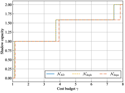
Figure 3: Comparison between the conventional no-signaling-assisted quantum communication and no-signaling-assisted shadow communication under different cost budgets. Compared with the quantum case, where the one-shot zero-error quantum capacities are $0$ for all channels, higher one-shot zero-error shadow capacity is achieved for every channel with increased cost budget.

In Figure 3, we present some numerical results on these channels at a low noise level ($p=0.9$). For conventional quantum communication with no-signaling codes, all these channels’ one-shot zero-error capacities are zero. For shadow communication, on the other hand, the one-shot zero-error capacities of these three channels steadily go up as the budget for sampling cost increases. The stepwise changes in the zero-error capacity show that we can trade in computational resources for better performance in shadow communication, attaining computational power beyond purely quantum protocols.

Appendix D Appendix D: Shadow Simulation via Noiseless Channels

In this section, we derive the SDP for $S^{(1)}_{\gamma,\rm NS}$, the one-shot zero-error $\gamma$-cost shadow simulation cost assisted by no-signaling codes. Along the way, we derive SDPs for some related quantities, which are of interest on their own.

To begin with, the minimum error and minimum sampling cost of shadow simulation with a noiseless channel can be solved by SDPs in Lemma 12. We omit the proof here as it is very similar to the proof of Lemma 9.

Lemma 12

For an identity channel ${\operatorname{id}}_{d}$ with dimension $d$ and a target quantum channel ${\cal M}_{A^{\prime}\to B^{\prime}}$, the minimum error of the simulation from ${\operatorname{id}}_{d}$ to ${\cal M}_{A^{\prime}\to B^{\prime}}$ assisted by ${\rm NS}$ codes with a cost budget $\gamma$ is given by the following SDP:

$$\varepsilon^{*}_{\gamma,\rm NS}({\operatorname{id}}_{d},{\cal N})=\inf \;\varepsilon$$ (D1a)

s.t. $$\;Z_{A^{\prime}B^{\prime}}\geq 0,~{}Z_{A^{\prime}B^{\prime}}\geq J^{\cal M}_{A^{\prime}B^{\prime}}-Y^{+}_{A^{\prime}B^{\prime}}+Y^{-}_{A^{\prime}B^{\prime}},$$ (D1b)

$$\;{\sf Tr}_{B^{\prime}}[Z_{A^{\prime}B^{\prime}}]\leq\frac{1}{2}\left(2\varepsilon+1-\frac{{\sf Tr}\left[V^{+}_{B^{\prime}}-V^{-}_{B^{\prime}}\right]}{d^{2}}\right)\mathbbm{1}_{A^{\prime}},$$ (D1c)

$$\;0\leq Y^{\pm}_{A^{\prime}B^{\prime}}\leq\mathbbm{1}_{A^{\prime}}\otimes V^{\pm}_{B^{\prime}},~{}{\sf Tr}_{B^{\prime}}\left[Y^{\pm}_{A^{\prime}B^{\prime}}\right]=\frac{{\sf Tr}\left[V^{\pm}_{B^{\prime}}\right]}{d^{2}}\mathbbm{1}_{A^{\prime}},~{}\frac{{\sf Tr}\left[V^{+}_{B^{\prime}}+V^{-}_{B^{\prime}}\right]}{d^{2}}\leq\gamma.$$ (D1d)

Similarly, the minimum sampling cost $\gamma_{\varepsilon,\rm NS}^{*}({\operatorname{id}}_{d},{\cal M}_{A^{\prime}\to B^{\prime}})$ with an error tolerance $\varepsilon$ is given by changing the optimization objective of the above SDP to ${\sf Tr}\left[V^{+}_{B^{\prime}}+V^{-}_{B^{\prime}}\right]/d^{2}$ and removing the condition ${\sf Tr}\left[V^{+}_{B^{\prime}}+V^{-}_{B^{\prime}}\right]/d^{2}\leq\gamma$.

Provided with Lemma 12, we now give an SDP for the zero-error minimum sampling cost of the shadow simulation of a noisy channel via a noiseless one.

Lemma 13

The zero-error minimum sampling cost of the shadow simulation of a channel ${\cal M}_{A^{\prime}\to B^{\prime}}$ via a $d$-dimensional identity channel ${\operatorname{id}}_{d}$ assisted by ${\rm NS}$ codes is given by the following SDP:

$$\gamma_{0,\rm NS}^{*}({\operatorname{id}}_{d},{\cal M}_{A^{\prime}\to B^{\prime}})=\inf \;\frac{{\sf Tr}\left[V^{+}_{B^{\prime}}+V^{-}_{B^{\prime}}\right]}{d^{2}}$$ (D2a)

s.t. $$\;{\sf Tr}\left[V^{+}_{B^{\prime}}-V^{-}_{B^{\prime}}\right]=d^{2},~{}{\sf Tr}_{B^{\prime}}\left[R_{A^{\prime}B^{\prime}}\right]=\frac{{\sf Tr}\left[V^{-}_{B^{\prime}}\right]}{d^{2}}\mathbbm{1}_{A^{\prime}},$$ (D2b)

$$\;J^{\cal M}_{A^{\prime}B^{\prime}}+R_{A^{\prime}B^{\prime}}\leq\mathbbm{1}_{A^{\prime}}\otimes V^{+}_{B^{\prime}},~{}0\leq R_{A^{\prime}B^{\prime}}\leq\mathbbm{1}_{A^{\prime}}\otimes V^{-}_{B^{\prime}}$$ (D2c)

Proof.

As in the shadow communication setting, the zero-error simulation of the channel ${\cal M}$ requires $J^{\cal N}_{A^{\prime}B^{\prime}}=Y^{+}_{A^{\prime}B^{\prime}}-Y^{-}_{A^{\prime}B^{\prime}}$ and ${\sf Tr}\left[V^{+}_{B^{\prime}}-V^{-}_{B^{\prime}}\right]=d^{2}$ (see the proof of Lemma 10). The equalities ${\sf Tr}_{B^{\prime}}\left[Y^{\pm}_{A^{\prime}B^{\prime}}\right]=\frac{{\sf Tr}\left[V^{\pm}_{B^{\prime}}\right]}{d^{2}}\mathbbm{1}_{A^{\prime}}$ in condition (D1d) can be equivalently written as

$${\sf Tr}_{B^{\prime}}\left[Y^{+}_{A^{\prime}B^{\prime}}+Y^{-}_{A^{\prime}B^{\prime}}\right]=\frac{{\sf Tr}\left[V^{+}_{B^{\prime}}+V^{-}_{B^{\prime}}\right]}{d^{2}}\mathbbm{1}_{A^{\prime}}\quad\text{and}\quad{\sf Tr}_{B^{\prime}}\left[Y^{+}_{A^{\prime}B^{\prime}}-Y^{-}_{A^{\prime}B^{\prime}}\right]=\frac{{\sf Tr}\left[V^{+}_{B^{\prime}}-V^{-}_{B^{\prime}}\right]}{d^{2}}\mathbbm{1}_{A^{\prime}}.$$ (D3)

Note that the latter equality ${\sf Tr}_{B^{\prime}}\left[Y^{+}_{A^{\prime}B^{\prime}}-Y^{-}_{A^{\prime}B^{\prime}}\right]={\sf Tr}\left[V^{+}_{B^{\prime}}-V^{-}_{B^{\prime}}\right]\mathbbm{1}_{A^{\prime}}/d^{2}$ can be removed because it is already implied by $J^{\cal N}_{A^{\prime}B^{\prime}}=Y^{+}_{A^{\prime}B^{\prime}}-Y^{-}_{A^{\prime}B^{\prime}}$ and ${\sf Tr}\left[V^{+}_{B^{\prime}}-V^{-}_{B^{\prime}}\right]=d^{2}$ with the observation that ${\sf Tr}_{B^{\prime}}\left[J^{\cal N}_{A^{\prime}B^{\prime}}\right]=\mathbbm{1}_{A^{\prime}}$ for ${\cal N}$ being a quantum channel. Hence, we arrive at the following SDP:

$$\gamma_{0,\rm NS}^{*}({\operatorname{id}}_{d},{\cal M}_{A^{\prime}\to B^{\prime}})=\inf \;\frac{{\sf Tr}\left[V^{+}_{B^{\prime}}+V^{-}_{B^{\prime}}\right]}{d^{2}}$$ (D4a)

s.t. $$\;J^{\cal M}_{A^{\prime}B^{\prime}}=Y^{+}_{A^{\prime}B^{\prime}}-Y^{-}_{A^{\prime}B^{\prime}},~{}{\sf Tr}\left[V^{+}_{B^{\prime}}-V^{-}_{B^{\prime}}\right]=d^{2},$$ (D4b)

$$\;0\leq Y^{\pm}_{A^{\prime}B^{\prime}}\leq\mathbbm{1}_{A^{\prime}}\otimes V^{\pm}_{B^{\prime}},~{}{\sf Tr}_{B^{\prime}}\left[Y^{+}_{A^{\prime}B^{\prime}}+Y^{-}_{A^{\prime}B^{\prime}}\right]=\frac{{\sf Tr}\left[V^{+}_{B^{\prime}}+V^{-}_{B^{\prime}}\right]}{d^{2}}\mathbbm{1}_{A^{\prime}}.$$ (D4c)

Denoting $R_{A^{\prime}B^{\prime}}\coloneqq Y^{-}_{A^{\prime}B^{\prime}}$, writing $Y^{+}_{A^{\prime}B^{\prime}}$ as $J^{\cal M}_{A^{\prime}B^{\prime}}+R_{A^{\prime}B^{\prime}}$, and exploiting ${\sf Tr}_{B^{\prime}}\left[J^{\cal M}_{A^{\prime}B^{\prime}}\right]=\mathbbm{1}_{A^{\prime}}$, one can obtain the claimed SDP.     $\sqcap$$\sqcup$

From this lemma, we can arrive at the following SDP for the one-shot zero-error $\gamma$-cost shadow simulation cost.

Theorem 14

The one-shot zero-error $\gamma$-cost simulation cost of a quantum channel ${\cal M}_{A^{\prime}\to B^{\prime}}$ assisted by no-signaling codes is given by the following SDP:

$$S^{(1)}_{\gamma,\rm NS}({\cal M})=\inf \;\log_{2}~{}\left\lceil\sqrt{{\sf Tr}\left[V_{B^{\prime}}\right]}\right\rceil$$ (D5a)

s.t. $$\;J^{\cal M}_{A^{\prime}B^{\prime}}+R_{A^{\prime}B^{\prime}}\leq\mathbbm{1}_{A^{\prime}}\otimes\frac{\gamma+1}{2}V_{B^{\prime}},~{}0\leq R_{A^{\prime}B^{\prime}}\leq\mathbbm{1}_{A^{\prime}}\otimes W_{B^{\prime}},$$ (D5b)

$$\;{\sf Tr}_{B^{\prime}}\left[R_{A^{\prime}B^{\prime}}\right]=\frac{\gamma-1}{2}\mathbbm{1}_{A^{\prime}},~{}{\sf Tr}\left[W_{B^{\prime}}\right]=\frac{\gamma-1}{2}{\sf Tr}\left[V_{B^{\prime}}\right].$$ (D5c)

Proof.

According to the SDP given in Lemma 13, we can write the one-shot simulation cost $S^{(1)}_{\gamma,\rm NS}({\cal M})$ as an optimization problem by substituting $d^{2}$ with ${\sf Tr}\left[V^{+}_{B^{\prime}}-V^{-}_{B^{\prime}}\right]$:

$$S^{(1)}_{\gamma,\rm NS}({\cal M})=\inf \;\log_{2}~{}\left\lceil\sqrt{{\sf Tr}\left[V^{+}_{B^{\prime}}-V^{-}_{B^{\prime}}\right]}\right\rceil$$ (D6a)

s.t. $$\;{\sf Tr}_{B^{\prime}}\left[R_{A^{\prime}B^{\prime}}\right]=\frac{{\sf Tr}\left[V^{-}_{B^{\prime}}\right]}{{\sf Tr}\left[V^{+}_{B^{\prime}}-V^{-}_{B^{\prime}}\right]}\mathbbm{1}_{A^{\prime}},~{}\frac{{\sf Tr}\left[V^{+}_{B^{\prime}}+V^{-}_{B^{\prime}}\right]}{{\sf Tr}\left[V^{+}_{B^{\prime}}-V^{-}_{B^{\prime}}\right]}\leq\gamma,$$ (D6b)

$$\;J^{\cal M}_{A^{\prime}B^{\prime}}+R_{A^{\prime}B^{\prime}}\leq\mathbbm{1}_{A^{\prime}}\otimes V^{+}_{B^{\prime}},~{}0\leq R_{A^{\prime}B^{\prime}}\leq\mathbbm{1}_{A^{\prime}}\otimes V^{-}_{B^{\prime}}.$$ (D6c)

Note that the inequality in condition (D6b) can be restricted to equality while keeping the optimized value unchanged. This is true because if $R_{A^{\prime}B^{\prime}}$ and $\bar{V}^{\pm}_{B^{\prime}}$ is a set of optimal solution with ${\sf Tr}\left[V^{+}_{B^{\prime}}+V^{-}_{B^{\prime}}\right]/{\sf Tr}\left[\bar{V}^{+}_{B^{\prime}}-\bar{V}^{-}_{B^{\prime}}\right]=\bar{\gamma}<\gamma$, then $R^{\prime}_{A^{\prime}B^{\prime}}\coloneqq R_{A^{\prime}B^{\prime}}+(\gamma-\bar{\gamma})\mathbbm{1}_{A^{\prime}B^{\prime}}/2d_{B^{\prime}}$ and $\bar{V}^{\prime\pm}_{B^{\prime}}\coloneqq\bar{V}^{\pm}_{B^{\prime}}+(\gamma-\bar{\gamma}){\sf Tr}\left[\bar{V}^{+}_{B^{\prime}}-\bar{V}^{-}_{B^{\prime}}\right]\mathbbm{1}_{B^{\prime}}/2d_{B^{\prime}}$ also form a set of optimal solution such that ${\sf Tr}\left[\bar{V}^{\prime+}_{B^{\prime}}+\bar{V}^{\prime-}_{B^{\prime}}\right]/{\sf Tr}\left[\bar{V}^{\prime+}_{B^{\prime}}-\bar{V}^{\prime-}_{B^{\prime}}\right]=\gamma$. Note that for $\bar{R}^{\prime\pm}_{A^{\prime}B^{\prime}}$ and $\bar{V}^{\prime\pm}_{B^{\prime}}$ to be valid solution, it must be true that ${\sf Tr}\left[\bar{V}^{+}_{B^{\prime}}-\bar{V}^{-}_{B^{\prime}}\right]\geq 1$ so that $\mathbbm{1}_{A^{\prime}}\otimes\bar{V}^{\prime-}_{B^{\prime}}\geq\bar{R}^{\prime}_{A^{\prime}B^{\prime}}$. This is indeed the case because from the constraint $R_{A^{\prime}B^{\prime}}\leq\mathbbm{1}_{A^{\prime}}\otimes V^{-}_{B^{\prime}}$ we have ${\sf Tr}_{B^{\prime}}\left[\bar{R}_{A^{\prime}B^{\prime}}\right]\leq{\sf Tr}\left[\bar{V}^{-}_{B^{\prime}}\right]\mathbbm{1}_{A^{\prime}}$. For the equality ${\sf Tr}_{B^{\prime}}\left[\bar{R}_{A^{\prime}B^{\prime}}\right]={\sf Tr}\left[\bar{V}^{-}_{B^{\prime}}\right]\mathbbm{1}_{A^{\prime}}/{\sf Tr}\left[\bar{V}^{+}_{B^{\prime}}-\bar{V}^{-}_{B^{\prime}}\right]$ to hold, ${\sf Tr}\left[\bar{V}^{+}_{B^{\prime}}-\bar{V}^{-}_{B^{\prime}}\right]$ has to be larger than or equal to $1$.

By changing the inequality in condition (D6b) to ${\sf Tr}\left[V^{+}_{B^{\prime}}+V^{-}_{B^{\prime}}\right]/{\sf Tr}\left[V^{+}_{B^{\prime}}-V^{-}_{B^{\prime}}\right]=\gamma$, it follows that ${\sf Tr}[V^{-}_{B^{\prime}}]=(\gamma-1){\sf Tr}[V^{+}_{B^{\prime}}]/(\gamma+1)$ and thus ${\sf Tr}_{B^{\prime}}\left[R_{A^{\prime}B^{\prime}}\right]=(\gamma-1)\mathbbm{1}_{A^{\prime}}/2$. Changing the variables to $V_{B^{\prime}}\coloneqq 2V^{+}_{B^{\prime}}/(\gamma+1)$ and $W_{B^{\prime}}\coloneqq V^{-}_{B^{\prime}}$ gives the claimed SDP.     $\sqcap$$\sqcup$

Similar to the one-shot zero-error shadow capacity, the SDP above implies that $S{(1)}_{\gamma,\rm NS}$ is a generalization of the no-signaling-assisted one-shot zero-error quantum simulation cost $S{(1)}_{\rm NS}$ as it reduces to the SDP for the latter Duan and Winter (2015); Fang et al. (2019) when $\gamma=1$. To showcase the difference between $S{(1)}_{\gamma,\rm NS}$ and $S{(1)}_{\rm NS}$, we consider the two-qubit amplitude damping channel ${\cal N}_{\rm AD}$, the two-qubit dephasing channel ${\cal N}_{\rm deph}$, and the two-qubit depolarizing channel ${\cal N}_{\rm depo}(\cdot)=p(\rho)+(1-p)\mathbbm{1}_{4}/4$, where $\mathbbm{1}_{4}$ denotes the four-dimensional identity operator, the parameter $p\in[0,1]$ indicates the level of noise, and by a two-qubit amplitude damping channel we mean two single-qubit amplitude damping channels with the same noise parameter acting independently on two qubits.

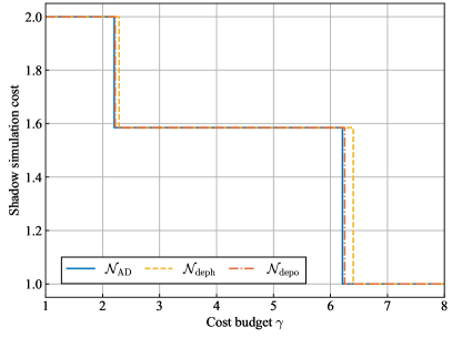
Figure 4: Comparison between the conventional no-signaling-assisted one-shot zero-error quantum simulation cost $S^{(1)}_{\rm NS}$ and no-signaling-assisted one-shot zero-error shadow simulation cost $S^{(1)}_{\gamma,\rm NS}$ under different cost budgets $\gamma$. Compared with the quantum case, where the simulation cost is $2$ for all channels, lower simulation cost is achieved for each channel with increased cost budget.

As in the task of shadow communication, we present numerical results on these channels at a low noise level ($p=0.9$) in Figure 4. The zero-error simulation costs of these channels decrease from $2$ (quantum simulation cost) to $1$ with increased cost budget. Again, the stepwise changes in the zero-error simulation cost show that we can attain computational power beyond purely quantum protocols by trading in more computational resources.

In the main text, we presented the minimum sampling cost of simulating a high-dimensional identity channel with a low-dimensional one. Now, we prove this result.

Theorem 3

Given identity channels ${\operatorname{id}}_{d}$ and ${\operatorname{id}}_{d^{\prime}}$ with $d^{\prime}\geq d\geq 2$, the minimum sampling cost of an exact shadow simulation of ${\operatorname{id}}_{d^{\prime}}$ using ${\operatorname{id}}_{d}$ and no-signaling resources is

$$\gamma^{*}_{0,\rm NS}\left({\operatorname{id}}_{d},{\operatorname{id}}_{d^{\prime}}\right)=2\left(\frac{d^{\prime}}{d}\right)^{2}-1.$$ (D7)

Proof.

The Choi operators of the noiseless channel ${\operatorname{id}}_{d}$ from system $A$ to system $B$ and the noiseless channel ${\operatorname{id}}_{d^{\prime}}$ from system $A^{\prime}$ to system $B^{\prime}$ are $J^{{\operatorname{id}}_{d}}_{AB}=\Gamma_{AB}$ and $J^{{\operatorname{id}}_{d^{\prime}}}_{A^{\prime}B^{\prime}}=\Gamma_{A^{\prime}B^{\prime}}$, respectively. It is straightforward to verify that

$$\bar{V}^{+}_{B^{\prime}}=d^{\prime}\mathbbm{1}_{B^{\prime}},\quad\bar{V}^{-}_{B^{\prime}}=\frac{d^{\prime 2}-d^{2}}{d^{\prime}}\mathbbm{1}_{B^{\prime}},\quad\bar{R}_{A^{\prime}B^{\prime}}=\frac{d^{\prime}(d^{\prime 2}-d^{2})}{(d^{\prime 2}-1)d^{2}}\mathbbm{1}_{A^{\prime}B^{\prime}}-\frac{d^{\prime 2}-d^{2}}{(d^{\prime 2}-1)d^{2}}\Gamma_{A^{\prime}B^{\prime}}$$ (D8)

form a feasible solution to the SDP for $\gamma_{0,\rm NS}^{*}({\operatorname{id}}_{d},{\operatorname{id}}_{d}^{\prime})$ as given in Lemma 13, implying

$$\gamma_{0,\rm NS}^{*}({\operatorname{id}}_{d},{\operatorname{id}}_{d}^{\prime})\leq\frac{1}{d^{2}}{\sf Tr}\left[\bar{V}^{+}_{B^{\prime}}+\bar{V}^{-}_{B^{\prime}}\right]=\frac{2d^{\prime 2}}{d^{2}}-1.$$ (D9)

Using the Lagrange dual function, we can derive that the following problem is the dual problem associated with SDP (D2):

$$\gamma_{0,\rm NS}^{*}({\operatorname{id}}_{d},{\cal M}_{A^{\prime}\to B^{\prime}})\geq\sup \;{\sf Tr}\left[M_{A^{\prime}B^{\prime}}J^{\cal M}_{A^{\prime}B^{\prime}}\right]-\lambda$$ (D10a)

s.t. $$\;M_{A^{\prime}B^{\prime}}\geq 0,~{}N_{A^{\prime}B^{\prime}}\geq 0,~{}M_{A^{\prime}B^{\prime}}+N_{A^{\prime}B^{\prime}}+K_{A^{\prime}}\otimes\mathbbm{1}_{B^{\prime}}\geq 0,$$ (D10b)

$$\;d^{2}{\sf Tr}_{A^{\prime}}\left[M_{A^{\prime}B^{\prime}}\right]=(1+\lambda)\mathbbm{1}_{B^{\prime}},~{}d^{2}{\sf Tr}_{A^{\prime}}\left[N_{A^{\prime}B^{\prime}}\right]=(1-\lambda-{\sf Tr}\left[K_{A^{\prime}}\right])\mathbbm{1}_{B^{\prime}}.$$ (D10c)

It is straightforward to verify that

$$\bar{\lambda}=1,\quad\bar{M}_{A^{\prime}B^{\prime}}=\frac{2}{d^{2}}\Gamma_{A^{\prime}B^{\prime}},\quad\bar{N}_{A^{\prime}B^{\prime}}=0,\quad\bar{K}_{A^{\prime}}=0.$$ (D11)

form a feasible solution to the dual problem for $\gamma_{0,\rm NS}^{*}({\operatorname{id}}_{d},{\operatorname{id}}_{d^{\prime}})$, implying

$$\gamma_{0,\rm NS}^{*}({\operatorname{id}}_{d},{\operatorname{id}}_{d^{\prime}})\geq{\sf Tr}\left[\bar{M}_{A^{\prime}B^{\prime}}J^{{\operatorname{id}}_{d^{\prime}}}_{A^{\prime}B^{\prime}}\right]-\bar{\lambda}=\frac{2d^{\prime 2}}{d^{2}}-1.$$ (D12)

Combining Eqs. (D9) and (D12), we conclude that

$$\gamma_{0,\rm NS}^{*}({\operatorname{id}}_{d},{\operatorname{id}}_{d}^{\prime})=\frac{2d^{\prime 2}}{d^{2}}-1,$$ (D13)

which completes the proof.     $\sqcap$$\sqcup$