Super-exponential quantum advantage for finding the center of a sphere

Abstract

This article considers the geometric problem of finding the center of a sphere in vector space over finite fields, given samples of random points on the sphere. We propose a quantum algorithm based on continuous-time quantum walks that needs only a constant number of samples to find the center. We also prove that any classical algorithm for the same task requires approximately as many samples as the dimension of the vector space, by a reduction to an old and basic algebraic result—Warning’s second theorem. Thus, a super-exponential quantum advantage is revealed for the first time for a natural and intuitive geometric problem.

Introduction.— A primary goal of quantum computing is to identify problems for which quantum algorithms can offer speedups over their classical counterpart. Grover’s algorithm [1] offers a quadratic speedup for unstructured database search problem. Shor’s algorithm [2] is exponentially faster than the best classical algorithm in factoring integers. Recent studies have also found exponential speedups in specific problems such as simulating the coupled oscillators [3], traversing a decorated welded-tree graph using adiabatic quantum computation [4], a graph property testing problem in the adjacency list model [5], a classification problem for quantum kernel methods based on discrete logarithm problem [6], a specific NP search problem based on random black-box function [7], and so on. However, to the best of our knowledge, no one has ever found a geometric problem that exhibits sharp quantum speedups.

In this letter, we consider a natural geometric problem of finding the center of a sphere given samples of random points on the sphere. To illustrate this problem, we begin with an intuitive example: if we want to pin down a circle on a paper, we will need $3$ points ($A,B,C$) which are not on the same line, as depicted in Fig. 1 (a); and if we want to fix an inflatable balloon, we will need $4$ points ($A,B,C,D$) which are not on the same plane, as depicted in Fig. 1 (b). As such, $n+1$ points are required to determine a sphere in $\mathbb{R}^{n}$.

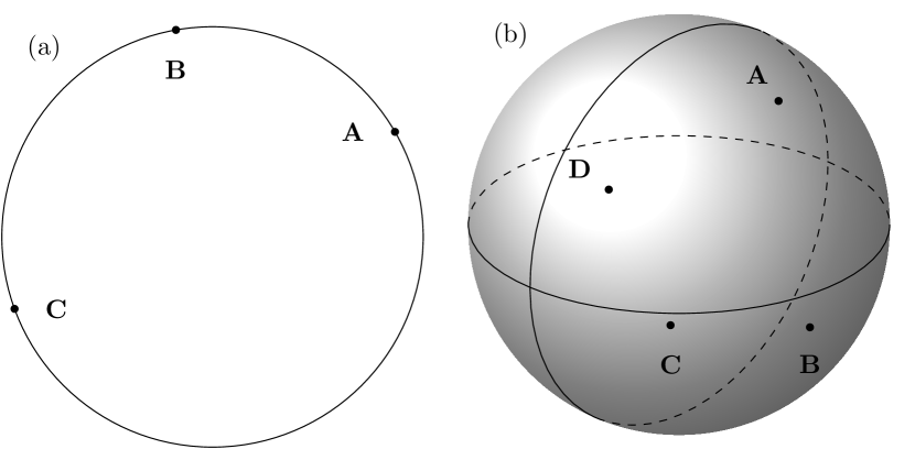
Figure 1: Spheres in the $\mathbb{R}^{2}$ and $\mathbb{R}^{3}$.

To accommodate the discrete nature of qubit-based quantum computer, we will replace the continuous vector space $\mathbb{R}^{n}$ with $\mathbb{F}_{q}^{n}$, the vector space over a finite field $\mathbb{F}_{q}$ with $q$ being a prime number. Define the length of a vector $x=(x_{1},\cdots,x_{n})\in\mathbb{F}_{q}^{n}$ by $l(x):=\sum_{j=1}^{n}x_{j}^{2}$. Then a sphere with radius $r\in\mathbb{F}_{q}\setminus\{0\}$ and center $t\in\mathbb{F}_{q}^{n}$ is denoted by $S_{r}+t=\{x+t\mid x\in S_{r}\}$, where

$$S_{r}:=\{x\mid x\in\mathbb{F}_{q}^{n},l(x)=r\}.$$ (1)

The problem is then formally described as follows.

Problem 1.

Find the unknown center $t\in\mathbb{F}_{q}^{n}$ of the sphere $S_{r}+t$ ($r>0$ is given) with as few samples of points on $S_{r}+t$ as possible.

In analogy to sampling a point uniformly random from $S_{r}+t$, each usage of the state $\ket{S_{r}+t}:=\frac{1}{\sqrt{s_{r}}}\sum_{v\in S_{r}+t}\ket{v}$, where $s_{r}:=|S_{r}|$, is regarded as a quantum sample. In this letter, we obtain the following theorem.

Theorem 1.

There is a quantum algorithm that solves Problem 1 with bounded error, and uses $O(\log q)$ samples. However, any classical algorithm that solves Problem 1 with bounded error requires $\Omega(n)$ samples.

Note that when $q$ is fixed to be a constant, the quantum algorithm needs constant $O(1)$ samples, while any classical algorithm requires $\Omega(n)$ samples. This is actually a super-exponential speedup because the classical $\Omega(n)$ v.s. quantum $O(\log n)$ separation is already an exponential speedup.

To prove the classical lower bound $\Omega(n)$, we find unexpectedly that it can be reduced to a basic algebraic theorem proved around 1935 by Warning [9], which gives a lower bound on the number of zeros of multi-variable polynomials over finite fields. We then design the quantum algorithm based on a continuous-time quantum walk (CTQW) on the Euclidean graph on $\mathbb{F}_{q}^{n}$, where two points $x,y$ are connected if and only if $l(x-y)=r$.

Quantum walks are an analogy to classical random walks, and have become a widely adopted paradigm to design quantum algorithms for various problems, such as spatial search [10, 11, 12, 13, 14], element distinctness [15], matrix product verification [16], triangle finding [17, 18], group commutativity [19], the welded-tree problem [20, 21, 22], and so on. There are two types of quantum walks: the CTQW and the discrete-time quantum walk (DTQW). CTQW is relatively simple, and mainly involves simulating a Hamiltonian $H$ that encodes the structure of the graph. DTQW is more diverse, ranging from the earliest and simplest coined quantum walk [23, 24] to various Markov chain based frameworks [25, 26, 27, 28, 29]. The quantum algorithm proposed in this letter is based on CTQW and is different from previous ones with sharp speedups featuring quantum Fourier transform, and thus our result may inspire the discovery of new quantum algorithms with sharp speedups.

Classical lower bound.— In the introduction section we have intuitively shown that $n+1$ points are required to determine a sphere in $\mathbb{R}^{n}$. Here we will rigorously prove that any classical algorithm requires $\Omega(n)$ samples of points on the sphere $S_{r}+t$ to determine the center $t$ with high probability. To prove this classical lower bound, we will use the following lemma, also known as Warning’s second theorem [30, 31, 32], attributed to Ewald Warning [9].

Lemma 1 (Warning’s second theorem).

Suppose $f_{1},f_{2},\cdots,f_{s}\in\mathbb{F}_{q}[x_{1},\cdots,x_{n}]$ are multivariate polynomials over $\mathbb{F}_{q}$ with $d_{i}=\text{deg}(f_{i})$. Let $d:=d_{1}+\cdots+d_{s}$ be the total degree and $V:=\{x=(x_{1},\cdots,x_{n})\in\mathbb{F}_{q}^{n}\mid f_{i}(x)=0,\forall\,1\leq i\leq s\}$ be the set of common zeros of $f_{i}$. Assume $n>d$ and $V\neq\emptyset$. Then $|V|\geq q^{n-d}$.

We can now obtain a relationship between the number of different points that a classical algorithm has sampled on $S_{r}+t$ and the upper bound of its success probability.

Lemma 2.

Suppose $c$ is a constant such that $0<c<1/2$. If a classical algorithm has sampled less than $cn$ different points on $S_{r}+t$, then it has at most $1/q^{(1-2c)n}$ probability of obtaining the correct center $t$.

Proof.

Denoted by $X+t$, where $X:=\{(x_{i1},\cdots,x_{in})\mid i=1,\ldots,s\}\subseteq S_{r}$, the $s\leq cn$ different points that the classical algorithm has obtained on $S_{r}+t$. We claim that there are at least $q^{(1-2c)n}$ possible centers $\{t^{\prime}\}\subseteq\mathbb{F}_{q}^{n}$ such that $X+t\subseteq S_{r}+t^{\prime}$. In other words, all of these possible spheres $\{S_{r}+t^{\prime}\}$ can lead to the same set of samples $X+t$. Having obtained only $X+t$, the algorithm cannot distinguish between the possible centers $\{t^{\prime}\}$, where only one of them is the correct center $t$. As $\left|\{t^{\prime}\}\right|\geq q^{(1-2c)n}$, the possibility of obtaining $t\in\{t^{\prime}\}$ is at most $1/q^{(1-2c)n}$.

To prove our claim, note that by letting $\bar{t}:=t^{\prime}-t$, the inclusion $X+t\subseteq S_{r}+t^{\prime}$ becomes $X\subseteq S_{r}+\bar{t}$, which results in the following system of polynomial equations over finite fields about variables $\bar{t}=(\bar{t}_{1},\cdots,\bar{t}_{n})$:

$$f_{i}:=\sum_{j=1}^{n}(x_{ij}-\bar{t}_{j})^{2}-r=0,\ 1\leq i\leq s.$$ (2)

Since $d_{i}=\text{deg}(f_{i})=2$ for all $i$, and $\bar{t}=\vec{0}$ is a solution (recall that $X\subseteq S_{r}$), the above equations have at least $q^{n-2s}\geq q^{(1-2c)n}$ common roots $\bar{t}$ by Lemma 1. Thus there are at least $q^{(1-2c)n}$ possible centers $t^{\prime}=\bar{t}+t$ such that $X+t\subseteq S_{r}+t^{\prime}$. ∎

If we let $c=1/3$, then a classical algorithm that has sampled less than $n/3$ different points on $S_{r}+t$ can only succeed with probability less than $1/q^{n/3}$, which is exponentially small. Therefore, if a classical algorithm wants to solve Problem 1 with high probability, $\Omega(n)$ samples are needed.

Quantum algorithm.— The quantum algorithm for Problem 1 is concise and consists of only four steps as shown below. The main idea is to use CTQW on the Euclidean graph $G$ on $\mathbb{F}_{q}^{n}$ to move amplitude from the sphere to its center. The Euclidean graph $G$ has vertex set $\mathbb{F}_{q}^{n}$, and two vertices $x,x^{\prime}\in F_{q}^{n}$ are connected by an undirected edge if and only if $l(x-x^{\prime})=r$.

The Hamiltonian $\bar{A}$ of the CTQW on the Euclidean graph $G$ is approximately the adjacency matrix $A$ of the Euclidean graph $G$, but with $A$’s largest eigenvalue $\lambda_{0}=s_{r}$ replaced by $0$. Specifically, $\bar{A}:=A-\lambda_{0}\ket{\widetilde{0}}\bra{\widetilde{0}}$, where $\ket{\tilde{0}}$ is the corresponding eigenvector of eigenvalue $\lambda_{0}$ and it is the equal superposition of all points in $\mathbb{F}_{q}^{n}$ (see [33, Proposition 2] for the spectral decomposition of $A$). Note that $A$ is symmetric since the graph $G$ is undirected, so $\bar{A}$ is a valid Hamiltonian. We will see later from numerical simulation that $A$ itself as the Hamiltonian is good enough.

1. Prepare the quantum sample $\ket{S_{r}+t}=\frac{1}{\sqrt{s_{r}}}\sum_{v\in S_{r}+t}\ket{v}$.

2. Apply a CTQW $e^{i\bar{A}t_{0}}$ to $\ket{S_{r}+t}$ for time $t_{0}=1/\sqrt{q^{n-1}\log q}$, and then measure in the computational basis obtaining a point in $\mathbb{F}_{q}^{n}$.

3. Repeat the above two steps for $O(\log q)$ times.

4. Output the point with the highest frequency.

The following lemma lower bounds the success probability of step 2. It can be seen as a fine-grained version of [34, Lemma 4].

Lemma 3.

The final state $\ket{\psi_{t_{0}}}:=e^{i\bar{A}t_{0}}\ket{S_{r}+t}$ of CTQW on the Euclidean graph $G$ has the following properties:

$$\left|\braket{x}{\psi_{t_{0}}}\right|\begin{cases}\leq O(q^{-(n-1)/2})&\text{for}\,x\neq t,\\ \geq\frac{h(q,n)}{\sqrt{\log q}}&\text{for}\,x=t,\end{cases}$$ (3)

where the function $h(q,n)$ is monotonically increasing in both $q$ and $n$, and $h(127,8)\geq 0.0016$.

From Lemma 3, the probability to obtain the center $t$ is $\Omega(1/\log q)$ in step 2, while the probability to obtain any point other than $t$ is exponentially small. Step 3 then guarantees the center $t$ to be found with high probability. Overall, the quantum algorithm needs $O(\log q)$ samples.

Proof of Lemma 3.

As shown in Appendix, the CTQW $e^{i\bar{A}t_{0}}=\sum_{k=0}^{\infty}\frac{(it_{0})^{k}}{k!}\bar{A}^{k}$ has a $(q+1)$-dimensional invariant subspace $\mathcal{H}_{0}$ spanned by the following orthonormal basis:

$$\mathcal{B}_{0}=\{\ket{t},\ket{S_{0}+t},\ket{S_{1}+t},\cdots,\ket{S_{q-1}+t}\},$$ (4)

where $S_{0}:=\{v\in\mathbb{F}_{q}^{n}:l(v)=0\}\setminus\{\vec{0}\}$ (see Eq. (1) for $S_{r}$ with $r\neq 0$). The following equation [33, Theorem 1] shows that $s_{r}:=|S_{r}|\approx q^{n-1}$ for all $r\in\mathbb{F}_{q}$.

$$s_{r} =\begin{cases}q^{n-1}+\chi((-1)^{\frac{n-1}{2}}r)q^{\frac{n-1}{2}}&n\,\mathrm{odd},r\neq 0,\\ q^{n-1}-\chi((-1)^{\frac{n}{2}})q^{\frac{n-2}{2}}&n\,\mathrm{even},r\neq 0,\\ q^{n-1}-1&n\,\mathrm{odd},r=0,\\ q^{n-1}+\chi((-1)^{\frac{n}{2}})(q-1)q^{\frac{n-2}{2}}-1&n\,\mathrm{even},r=0,\end{cases}$$ (5)

where $\chi(a)\in\{0,1,-1\}$ indicates whether $a$ is zero, or the square of some element in $\mathbb{F}_{q}$, or otherwise.

We first consider $x\neq t$. Since $\ket{\psi_{t_{0}}}\in\mathrm{span}\,\mathcal{B}_{0}$, we have:

$$\left|\braket{x}{\psi_{t_{0}}}\right| \leq\max_{r^{\prime}\in[q]}\left|\braket{x}{S_{r^{\prime}}+t}\right|$$ (6)

$$=\max_{r^{\prime}\in[q]}1/\sqrt{s_{r^{\prime}}}=O(q^{-(n-1)/2}).$$ (7)

We then consider the lower bound of $\left|\braket{t}{\psi_{t_{0}}}\right|$ as follows:

$$\left|\braket{t}{\psi_{t_{0}}}\right|=\left|\bra{t}e^{i\bar{A}t_{0}}\ket{S_{r}+t}\right|=\left|\bra{t}\sum_{k=0}^{\infty}\frac{(it_{0})^{k}}{k!}\bar{A}^{k}\ket{S_{r}+t}\right|$$ (8)

$$\geq t_{0}\bra{t}\big{(}A-\lambda_{0}\ket{\widetilde{0}}\bra{\widetilde{0}}\big{)}\ket{S_{r}+t}-\sum_{k=2}^{\infty}\frac{t_{0}^{k}}{k!}\left|\bra{t}\bar{A}^{k}\ket{S_{r}+t}\right|$$ (9)

$$\geq t_{0}\left(\sqrt{s_{r}}-s_{r}\frac{\sqrt{s_{r}}}{\sqrt{q^{n}}}\frac{1}{\sqrt{q^{n}}}\right)-\sum_{k=2}^{\infty}\frac{(2t_{0}\sqrt{q^{n-1}})^{k}}{k!}$$ (10)

$$=\sqrt{s_{r}t_{0}^{2}}-\frac{s_{r}}{q^{n}}\sqrt{s_{r}t_{0}^{2}}-(e^{2t_{0}\sqrt{q^{n-1}}}-1-2t_{0}\sqrt{q^{n-1}}).$$ (11)

We have used $\braket{t}{S_{r}+t}=0$ and the triangle inequality $|x+y|\geq|x|-|y|$ and the fact that $\bar{A}=A-\lambda_{0}\ket{\widetilde{0}}\bra{\widetilde{0}}$ is a real matrix in Formula (9). Formula (10) is because the adjacency matrix $A$ maps $\ket{t}$ to $\sqrt{s_{r}}\ket{S_{r}+t}$, and $|\bra{t}\bar{A}^{k}\ket{S_{r}+t}|\leq\|\bar{A}^{k}\|\leq(2\sqrt{q^{n-1}})^{k}$, where the second upper bound follows from the fact that the spectral radius of $\bar{A}$ is less than $2\sqrt{q^{n-1}}$ [33, Theorem 3].

From Eq. (5) we know $q^{n-1}-q^{(n-1)/2}\leq s_{r}\leq q^{n-1}+q^{(n-1)/2}$. Recall that $t_{0}=1/\sqrt{q^{n-1}\log q}$. Thus we have $\frac{1}{\log q}(1-\frac{1}{q^{(n-1)/2}})\leq s_{r}\,t_{0}^{2}\leq\frac{1}{\log q}(1+\frac{1}{q^{(n-1)/2}})$, and $s_{r}/q^{n}\leq\frac{1}{q}(1+\frac{1}{q^{(n-1)/2}})$. Using basic inequalities $\sqrt{a-\varepsilon}\geq\sqrt{a}-\sqrt{\varepsilon}$ and $\sqrt{a+\varepsilon}\leq\sqrt{a}+\sqrt{\varepsilon}$, we can continue to calculate the lower bound of $\left|\braket{t}{\psi_{t_{0}}}\right|$ as follows:

$$\left|\braket{t}{\psi_{t_{0}}}\right|\geq\frac{1}{\sqrt{\log q}}(1-\frac{1}{q^{(n-1)/4}})$$

$$\quad-\frac{1}{\sqrt{\log q}}(1+\frac{1}{q^{(n-1)/4}})(\frac{1}{q}+\frac{1}{q^{(n+1)/2}})$$

$$\quad-(e^{2/\sqrt{\log q}}-1-\frac{2}{\sqrt{\log q}})$$ (12)

$$\geq\frac{1}{\sqrt{\log q}}(1-\frac{1}{q}-\frac{4}{q^{(n-1)/4}}-g(\sqrt{\log q}))$$ (13)

$$:=\frac{1}{\sqrt{\log q}}h(q,n)$$ (14)

In Formula (13), $g(x):=xe^{2/x}-x-2$ is monotonically decreasing when $x>0$, and $g(\sqrt{\log q})<1$ when $q\geq 127$. Thus $h(q,n)$ is monotonically increasing in both $q$ and $n$, and it can be verified that $h(127,8)\geq 0.0016$. ∎

Numerical simulation.— To illustrate that $A$ is good enough as the Hamiltonian, we consider the simplest cases where the size of the finite field is $q=3$ and the radius of the sphere is $r=1$. The invariant subspace $\mathcal{H}_{0}=\text{span}\,\mathcal{B}_{0}$ of CTQW $e^{iAt_{0}}$ is then $4$-dimensional: $\mathcal{B}_{0}=\{\ket{t},\ket{S_{0}+t},\ket{S_{1}+t},\ket{S_{2}+t}\}$.

We first consider the case where $n=5$. Using Lemma 4 in Appendix, we have the following matrix expression of $A$ on the basis $\mathcal{B}_{0}$.

$$M_{A}=\begin{bmatrix}0&0&3\sqrt{10}&0\\ 0&27&24\sqrt{2}&9\sqrt{10}\\ 3\sqrt{10}&24\sqrt{2}&33&12\sqrt{5}\\ 0&9\sqrt{10}&12\sqrt{5}&30\end{bmatrix}.$$ (15)

Denote by $p(t_{1}):=\left|\bra{t}e^{iAt_{1}\cdot t_{0}}\ket{S_{r}+t}\right|^{2}$ the success probability of reaching the target state after time $t_{1}\cdot t_{0}$, then $p(t_{1})=\left|\bra{0}e^{iM_{A}t_{1}\cdot t_{0}}\ket{2}\right|^{2}$ for the case where $q=3,r=1,n=5$. By numerical calculation, we obtain $p(t_{1})$ with $t_{1}\in[0,10]$ as shown in Fig. 2. It shows that the success probability of the CTQW oscillates periodically with its evolution time, and the earliest time to achieve the maximum success probability is around $t_{1}=1.5$.

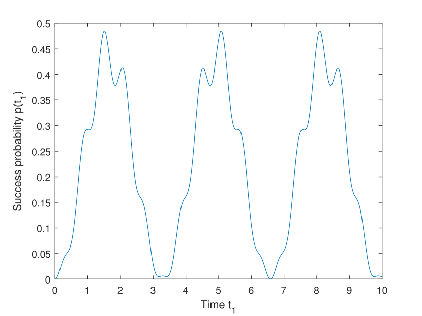
Figure 2: The success probability $p(t_{1})$ for the case where $q=3,r=1,n=5$.

We then consider the cases where $n=3\sim 12$. Fig. 3 shows that as the dimension $n$ varies, the optimal evolution time $t_{max}:=\mathop{\arg\max}\limits_{t_{1}\in[0,3]}p(t_{1})$ lies in $[1,2]$, and the corresponding maximum success probability $p(t_{max})\geq 0.4$.

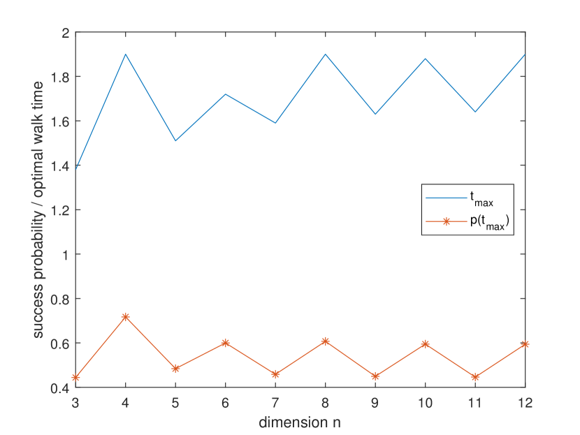
Figure 3: Optimal CTQW time $t_{max}$ and corresponding success probability $p(t_{max})$. Here, $q=3,r=1$, and $n=3\sim 12$.

In summary, we have found a super-exponential quantum advantage for a natural and geometric problem of finding the center of a sphere in $\mathbb{F}_{q}^{n}$ given samples on the sphere. While any classical bounded-error algorithm requires $\Omega(n)$ samples on the sphere, the quantum algorithm based on CTQW on the Euclidean graph on $\mathbb{F}_{q}^{n}$ needs only $O(1)$ sample.

This work is supported by the National Natural Science Foundation of China Grant No. 62272492, and the Guangdong Basic and Applied Basic Research Foundation Grant No. 2020B1515020050.

Appendix—We will prove the following Lemma 4, used in the proof of Lemma 3 and also in obtaining the reduced matrix $M_{A}$ in Eq. (15). Lemma 4 is extracted from [34, Lemma 4], but with a more detailed proof for the convenience of the reader. Lemma 4 implies that $\mathcal{H}_{0}$ is an invariant subspace of the CTQW $e^{i\bar{A}t_{0}}=\sum_{k=0}^{\infty}\frac{(it_{0})^{k}}{k!}\bar{A}^{k}$, since $\bar{A}=A-\lambda_{0}\ket{\widetilde{0}}\bra{\widetilde{0}}$, and $\sqrt{q^{n}}\ket{\tilde{0}}=\sum_{x\in\mathbb{F}_{q}^{n}}\ket{x}=\ket{t}+\sum_{r^{\prime}=0}^{q-1}\sqrt{s_{r^{\prime}}}\ket{S_{r^{\prime}}+t}\in\mathcal{H}_{0}$.

Lemma 4.

The adjacency matrix $A$ has a $(q+1)$-dimensional invariant subspace $\mathcal{H}_{0}$ spanned by the following orthonormal basis:

$$\mathcal{B}_{0}=\{\ket{t},\ket{S_{0}+t},\ket{S_{1}+t},\cdots,\ket{S_{q-1}+t}\}.$$ (16)

Specifically, we have

$$A\ket{t} =\sqrt{s_{r}}\ket{S_{r}+t},$$ (17)

$$A\ket{S_{r^{\prime}}+t} =c_{r^{\prime}}\ket{t}+\sum_{r^{\prime\prime}=0}^{q-1}c(r^{\prime\prime},r^{\prime})\ket{S_{r^{\prime\prime}}+t},$$ (18)

where $c(r^{\prime\prime},r^{\prime}):=\sqrt{\frac{s_{r^{\prime\prime}}}{s_{r^{\prime}}}}\left|S_{r}\cap(S_{r^{\prime}}+v_{0}^{\prime\prime})\right|$ for arbitrary $v_{0}^{\prime\prime}\in S_{r^{\prime\prime}}$, and $c_{r^{\prime}}:=\delta_{r^{\prime},r}\sqrt{s_{r}}$.

Proof.

Eq. (17) follows from the definition that $A$ maps any $x\in\mathbb{F}_{q}^{n}$ to $\{y\in F_{q}^{n}\mid l(y-x)=r\}=S_{r}+x$. To prove Eq. (18), we consider any point $v^{\prime\prime}+t$ on $S_{r^{\prime\prime}}+t$, where $v^{\prime\prime}\in S_{r^{\prime\prime}}$. We calculate

$$\bra{v^{\prime\prime}+t}A\ket{S_{r^{\prime}}+t}$$ (19)

$$=\frac{1}{\sqrt{s_{r^{\prime}}}}\sum_{v\in S_{r}}\sum_{v^{\prime}\in S_{r^{\prime}}}\braket{v^{\prime\prime}+t}{v-v^{\prime}+t}$$ (20)

$$=\frac{1}{\sqrt{s_{r^{\prime}}}}\left|S_{r}\cap(S_{r^{\prime}}+v^{\prime\prime})\right|.$$ (21)

We used $\ket{S_{r^{\prime}}+t}=\frac{1}{\sqrt{s_{r^{\prime}}}}\sum_{v^{\prime}\in S_{r^{\prime}}}\ket{-v^{\prime}+t}$ in Eq. (20), and Eq. (21) follows from the fact that the condition $v^{\prime\prime}+t=v-v^{\prime}+t$ is equivalent to $v=v^{\prime}+v^{\prime\prime}$, where $v\in S_{r}$ and $v^{\prime}\in S_{r^{\prime}}$.

We will later show that $\left|S_{r}\cap(S_{r^{\prime}}+v^{\prime\prime})\right|$ is the same for any $v^{\prime\prime}\in S_{r^{\prime\prime}}$. Thus we have

$$A\ket{S_{r^{\prime}}+t}$$ (22)

$$=c_{r^{\prime}}\ket{t}+\sum_{r^{\prime\prime}=0}^{q-1}\sum_{v^{\prime\prime}\in S_{r^{\prime\prime}}}\bra{v^{\prime\prime}+t}A\ket{S_{r^{\prime}}+t}\ket{v^{\prime\prime}+t}$$ (23)

$$=c_{r^{\prime}}\ket{t}+\sum_{r^{\prime\prime}=0}^{q-1}\frac{1}{\sqrt{s_{r^{\prime}}}}\left|S_{r}\cap(S_{r^{\prime}}+v_{0}^{\prime\prime})\right|\sum_{v^{\prime\prime}\in S_{r^{\prime\prime}}}\ket{v^{\prime\prime}+t}$$ (24)

$$=c_{r^{\prime}}\ket{t}+\sum_{r^{\prime\prime}=0}^{q-1}c(r^{\prime\prime},r^{\prime})\ket{S_{r}^{\prime\prime}+t}.$$ (25)

We used $\bra{t}A\ket{S_{r^{\prime}}+t}=\bra{S_{r^{\prime}}+t}A\ket{t}=\delta_{r^{\prime},r}\sqrt{s_{1}}$ in Eq. (23), where the first equality follows from $A$ being symmetric. In Eq. (24), $v_{0}^{\prime\prime}\in S_{r^{\prime\prime}}$ is arbitrary.

We now show that $\left|S_{r}\cap(S_{r^{\prime}}+v^{\prime\prime})\right|$ is the same for any $v^{\prime\prime}\in S_{r^{\prime\prime}}$, or equivalently, $|S_{r}\cap(S_{r^{\prime}}+x)|=|S_{r}\cap(S_{r^{\prime}}+z)|$ for any $x\in S_{r^{\prime\prime}}$ and $z\in S_{r^{\prime\prime}}$. We will later construct an isometry $\tau$ of $\mathbb{F}_{q}^{n}$ such that $z=\tau(x)$. As $\tau$ is a distance-preserving bijection, we have $\tau(S_{r})=S_{r}$ and $\tau(S_{r^{\prime}})=S_{r^{\prime}}$, and thus $\tau(S_{r}\cap(S_{r^{\prime}}+x))=S_{r}\cap(S_{r^{\prime}}+z)$, which implies $|S_{r}\cap(S_{r^{\prime}}+x)|=|S_{r}\cap(S_{r^{\prime}}+z)|$. The isometry $\tau$ can be constructed by extending the isometry $\tau^{\prime}:ax\mapsto az$ that maps subspace $U=\{ax:a\in\mathbb{F}_{q}\}$ to subspace $W=\{az:a\in\mathbb{F}_{q}\}$ (note that $U$ and $W$ are both $1$-dimensional subspace, since $x$ and $z$ are both nonzero points), to an isometry $\tau$ of the whole space $\mathbb{F}_{q}^{n}$ using Witt’s Lemma [35, Section 20]. ∎