Modeling Extreme Events: Univariate and Multivariate Data-Driven Approaches

Abstract

Modern inference in extreme value theory faces numerous complications, such as missing data, hidden covariates or design problems. Some of those complications were exemplified in the EVA 2023 data challenge. The challenge comprises multiple individual problems which cover a variety of univariate and multivariate settings. This note presents the contribution of team genEVA in said competition, with particular focus on a detailed presentation of methodology and inference.

1 Introduction

The importance of modeling, predicting and managing rare events continues to grow in an interconnected world. New and ongoing problems in climate, hydrological or financial applications require and inspire adaptive approaches, for example to plan against heatwaves, floods and financial crises, and to mitigate their potentially disastrous impacts. Modeling approaches for univariate extreme values often employ the Fisher–Tipett–Gnedenko theorem [15, 19], which under mild assumptions shows that the limititing distribution of the renormalized maximum of i.i.d. random variables follows the generalized extreme value distribution. A popular alternative to this approach is the peaks-over-threshold method [3, 33], which utilizes the convergence of scaled exceedances of a data generating process to a generalized Pareto distribution. Those approaches allow for theoretically justified extrapolation outside the range of observations, which in turn leads to a much better understanding of the behavior of rare events, especially for cases of unprecedented scale. For details we refer to Coles [5].

In many applications, understanding which magnitude an extreme event could take in the future is vital. This is achieved by estimating extreme quantiles, using one of the two approaches for extrapolation. As the occurrence of rare events often depends on several drivers, understanding how risk varies with its drivers is also essential for effective planning. Conditional quantile estimates are therefore an important complement to static return levels. For extreme levels, where only few data points are available, standard quantile regression methods [29] are only of limited use for estimating those conditional quantiles. This lead to the development of extreme quantile regression, which incorporates extreme value theory into quantile regression. Many classical approaches to extreme quantile regression use linear models [47, 31], generalized additive models [4, 48] or kernel methods [7, 16, 43]. However, those approaches typically suffer from limitations in either flexibility or covariate dimensionality. This motivated recent interest in more flexible and machine-learning based approaches to address more complex multivariate dependencies, for example using tree-based ensembles [44, 18, 30], or neural networks [32, 35, 1]. An application of extreme quantile regression with neural networks is discussed in Section 2.3. Providing reliable confidence intervals (CI) for extreme quantiles can be a difficult task, even for static estimates [49]. For complex dependence models, one usually relies on bootstrap methods [8, 9] to estimate covariate dependent CIs. Although bootstrap CIs are well understood for some extreme statistics [22], they are not for the more flexible covariate-dependent models. One main difficulty is the sensitivity of extreme value estimates on the most extreme observations, which can lead to unwanted discrete behaviors on the bootstrap samples.

When interest is in multivariate extremes, modeling and inference depends on the asymptotic dependence properties of the underlying data-generating process. A common assumption is multivariate regular variation [34], which allows for two related asymptotic models. The limit distribution of normalized maxima of i.i.d. random vectors is called a max-stable distribution [21]. Multivariate Pareto distributions are defined as the limit arising when conditioning on the exceedance of a high threshold, while properly renormalizing [37]. For extremal dependence modeling, the work of Heffernan and Tawn [24] introduced a very flexible approach, see for example Wadsworth et al [45] for a detailed discussion. Under the assumption of asymptotic dependence, the recent introduction of extremal conditional independence [12] allows the definition of graphical models in extremes. This innovation has sparked a new line of research in multivariate extremes see e.g. Engelke and Volgushev [14], Engelke and Ivanovs [13]. Here, particular focus is on parsimonious graphical models for the parametric Hüsler–Reiss family of multivariate Pareto distributions, see e.g. Wan and Zhou [46], Hentschel et al [25], Röttger et al [39].

The Extreme Value Analysis (EVA) 2023 data challenge [36] comprises four individual problems in extreme value statistics. The individual problems share similar complications motivated by real-world examples. In particular, the simulated data are compromised by common complications as missing data points, hidden covariates or design problems. This note provides a detailed summary of the modeling and inferential approaches of team genEVA, with particular focus on new or uncommon approaches. The team was ranked in third place overall (or in second place exaequo before the splitting rule).

The setting for the individual challenges are environmental data sets from a fictional planet. The meteorological data, which were simulated such that previous knowledge of climatic conditions on Earth is not useful for the analysis, are split into a univariate (for challenges C1 and C2) and a relatively high-dimensional setting (for challenges C3 and C4). Furthermore, no spatial information is provided for the analysis.

The rest of this note is structured in two major sections. Section 2 discusses the related quantile estimation challenges C1 and C2 and Section 3 the related joint-probability challenges C3 and C4. We give a detailed introduction to the respective setting and modeling approaches in each section.

2 Extreme Quantile Estimation

2.1 Goals and Data

One way to quantify the risk associated to a univariate variable $Y$ is using extreme quantiles, or return levels. They are a common risk measure in hydrology and environmental sciences where data is collected regularly, say yearly, or monthly, so the $T$-years return level: $q_{T}$, can be interpreted as the level we expect to exceed once every $T$ years. The quantity $q_{T}$ can be defined by

$$q_{T}=F_{Y}^{-1}\left(1-\frac{1}{Tn_{Y}}\right),$$

where $F_{Y}$ is the distribution of $Y$ and $n_{Y}$ are the number of measurements we collect per year. In this context, $T$ is referred to as the return period. Actually, as new observations of the variable $Y$ are recorded, they are likely to hit unprecedented levels. In this manner, return levels model how frequently the variable $Y$ reaches high levels. Return levels play an important role for designing risk plans, for example, the quantities reported by water-cycle analysis are of great interest to create policies aiming to protect the local communities against natural hazards as flooding. A full risk study then results from a balancing equation between the level of protection aimed for, and the cost associated to it. Overestimating the level typically incurs excessive expenses, and a misallocation of resources, but underestimating the risk can lead to catastrophic economic, societal and environmental consequences. We then see that the nature of the problem is asymmetric, as we can tolerate the extra cost to prevent the disastrous impact of natural catastrophes. To align with the real-life objectives in risk assessment, we consider an asymmetric loss function for a return level $q_{T}$ given by

$$L(q_{T},\hat{q}_{T})=\begin{cases}0.9(0.99q_{T}-\hat{q}_{T}),&\text{ if }0.99q_{T}>\hat{q}_{T}\\ 0,&\text{ if }|q_{T}-\hat{q}_{T}|\leq 0.01q_{T}\\ 0.1(\hat{q}_{T}-1.01q_{T}),&\text{ if }1.01q_{T}<\hat{q}_{T},\end{cases}$$ (1)

where $\hat{q}_{T}$ is an estimate of the true return level $q_{T}$. This asymmetric loss function is designed to penalize underestimation more compared to overestimation.

In numerous applications, the measurements of $Y$ are recorded together with a set of covariates relevant to predict $Y$. In this context, conditional extreme quantiles provide more in-depth understanding on how the extremal behavior of the variable changes as a response to covariates. The conditional quantile of $Y$ given a vector of observed covariates $\mathbf{X}=\mathbf{x}$ is defined as

$$Q_{\mathbf{x}}(\tau)=F^{-1}_{Y\mid\mathbf{X}=\mathbf{x}}(\tau),\quad\tau\in(0,1),$$ (2)

where $F^{-1}_{Y\mid\mathbf{X}=\mathbf{x}}$ the generalized inverse of the conditional distribution function of $Y\mid\mathbf{X}$, so that $\mathbb{P}\left(Y<Q_{\mathbf{x}}(\tau)\mid\mathbf{X}=\mathbf{x}\right)=\tau$. On one hand, if the probability level $\tau$ at which we aim to estimate the quantile is relatively extreme given the number of observations, extreme value statistics are essential for extrapolation. On the other hand, predicting quantiles conditionally requires regression methods. Extreme quantile regression methods are therefore a natural choice for estimating (2) in our context. We describe an extremal quantile regression method using neural networks in Section 2.3.2.

In the context of the 2023 data challenge competition for the extreme value analysis conference, each competing team was asked to analyze a synthetic dataset composed of $n=21,000$ observations $\{(\mathbf{x}_{i},y_{i})\}_{i=1}^{n}$ of the random vector $(\mathbf{X},Y)$, where $Y\in\mathbb{R}$ is the response variable and $\mathbf{X}\in\mathbb{R}^{p}$ is the vector of $p=8$ covariates. Observations from six of the eight covariates are missing completely at random in the training set. Further details about the variables and their meaning are given in Rohrbeck et al [36]. The goal of the first two competition challenges was to compute univariate extreme quantiles both conditional and unconditional on the covariates. For Task C2, the aim was to obtain an estimate $\hat{q}_{T}$ of the static return level $q_{T}$ satisfying $q_{T}=F_{Y}^{-1}(1-(6\times 10^{4})^{-1})$ that minimizes asymmetric loss (1). Our proposed methodology for this task is described and assessed first in Section 2.2. Additionally to the training data, we had a test dataset composed of $n_{t}=100$ new observations of the covariate vector $\mathbf{X}$ only. The goals for Task C1 are to estimate, for each covariate vector $\mathbf{x}$ in the test set,

1. the conditional quantile of $Y$, $Q_{\mathbf{x}}(\tau)$, at the extreme level $\tau=0.9999$, and

2. the corresponding central $50\%$ confidence interval (CI) for $Q_{\mathbf{x}}(\tau)$.

In the data competition, the performance for Task C1 was only assessed by how close the CI coverage of the true test response values was to 50%, with the average CI width used only as a tie-breaker [36]. Even though it is possible to get a perfect score by producing 50 very narrow and 50 very wide intervals, we focus on a methodology providing genuine 50% confidence intervals that are meaningful for each individual observation. Our proposed approach for this two-part task is discussed in Section 2.3.

2.2 Univariate quantile inference (Task C2)

Our goal in this section is to obtain reliable point estimates of high return levels which produce low values for the asymmetric loss function (1). For inference purposes, consider observations $Y_{1},\dots,Y_{n}$, and consider a sample-based confidence interval of the $T$-years return level where we denote $\hat{q}_{T}^{l}$ and $\hat{q}_{T}^{u}$ the lower and upper bounds of the confidence interval. To optimize the point estimate of the $T$-years return level based on the asymmetric loss, we trust the confidence interval to contain the true value, and we pick a point estimate inside the confidence interval by minimizing the expected loss:

$$\hat{q}_{T}^{op}(\lambda)=\left\{\operatorname*{arg\,min}_{q\in[\hat{q}_{T}^{l},\hat{q}_{T}^{u}]}\int_{q_{T}^{l}}^{q_{T}^{u}}L(s,q)\,ds\right\}-\lambda(q_{T}^{u}-q_{T}^{l}),$$ (3)

for $\lambda\geq 0$. The parameter $\lambda$ can be seen as a tuning parameter, when $\lambda=0$, it means we look for the safest choice, but if $\lambda>0$, we opt for a lower estimate, which can be seen as a riskier choice. To illustrate this strategy, we plot the loss function in Figure 1 evaluated at the values from a confidence interval. The true value is unknown, but we see that the higher values in the confidence interval have a smaller expected loss within the interval compared lo lower values of the confidence interval.

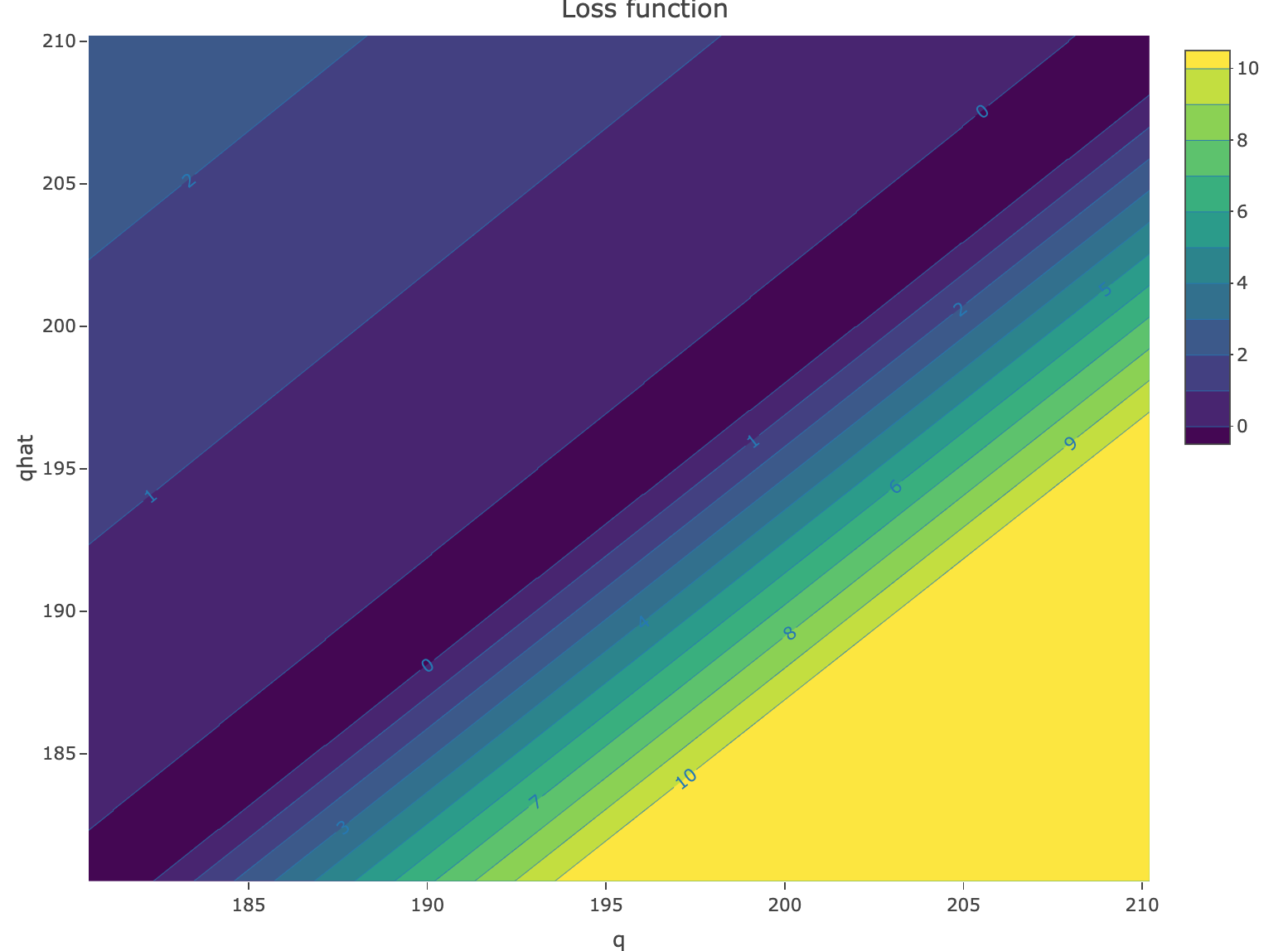
Figure 1: Heatmap of the loss function in (1) evaluated on points from a confidence interval $[\hat{q}_{T}^{\ell},\hat{q}_{T}^{u}]$ for the $T$-years return level $q_{T}$ of the response variable $Y$.

To obtain a first estimate of a high return level we rely on univariate extreme value statistics [cf. 5] and consider the peaks over threshold method, where, given a high threshold $u>0$, we fit the exceeded amounts with a generalized Pareto distribution, and then compute an estimate of the $T$-years return level as

$$\hat{q}_{T}=u+\frac{\hat{\sigma}}{\hat{\xi}}\left\{\left(\frac{n_{u}}{T\times n_{Y}\times n}\right)^{-\hat{\xi}}-1\right\},$$ (4)

where $n_{u}=\sum_{t=1}^{n}\mathds{1}(Y_{i}>u)$, $n_{Y}$ is the number of observations recorded per year, and $\hat{\sigma},\hat{\xi}$ are the parameters of the fitted generalized Pareto distribution. We can obtain these using profile maximum likelihood methods, and thus we can compute confidence intervals of the parameters estimates, and of the $T$-years return level $q_{T}$.

We focus on estimating the $200$-years return level $q_{200}$ based on $70$-years daily records. When the sample size is reasonably large, we can fine-tune the value of $\lambda$ performing a $k$-fold cross validation procedure that we describe next. We divide our sample into $k$ subsamples each of length $\lfloor n/k\rfloor$, and for each subsample we compute a $T$-years return level $\hat{q}_{T,i}$ and its confidence interval with $T=200/k$, for $i=1,\dots,k$. Then, we use the observations that do not belong to the $i$-th sample to compute the empirical $T$-return level that we denote $q_{T,i}$, and which we use as an approximation of the true value. The $k$-fold validation is introduced to compensate for the bias-variance tradeoff in extreme value statistics where choosing a high threshold $u$ in (4) decreases the effective sample size, but choosing a low threshold can produce biased estimates due to misspecification of the model when we approximate the distribution of exceeded amounts above a high threshold with a generalized Pareto distribution. Instead, the empirical quantiles always yield unbiased estimates of the $T-$years return level and thus can be used to help us fine-tune our point estimates. We use the empirical $T$-return level $q_{T,i}$ to compute $\lambda_{i}$ verifying $\hat{q}_{T}^{op}(\lambda_{i})=q_{T,i}$ with the notation in (3). Finally, we let $\lambda_{0}$ equal the median of the obtained values $\lambda_{1},\dots,\lambda_{k}$, and we return $\hat{q}_{200}^{op}(\lambda_{0})$ as the point estimate of the $200$-years return value.

2.2.1 Methodology assessment

To assess the performance of our fine-tuning algorithm we conduct a small numerical experiment which aims to compare the classic high return level point estimate obtained from the generalized Pareto distribution fit in (4), and the fine-tuned estimate obtained using (3) together with the $k$-fold cross validation strategy for extremes. In our experiments we consider different distributions in the domain of attraction of the generalized Pareto distribution, and for each distribution we also consider different sample sizes $n$. For a fixed sample length $n$, we then estimate the quantile $q$ such that $q=F_{Y}^{-1}(1-{70}/{(n\times 200)})$. To estimate this value and compute confidence intervals, we fit the generalized Pareto distribution to the exceeded amounts above the $95$th empirical percentile, and for fine-tuning we fix $k=7$ to run the $k$-fold cross-validation algorithm. Table 1 reports the obtained results. We see that fine-tuning the algorithm minimizes the expected asymmetric loss in all cases, and also helps to reduce the variance compared to the classic approach based on one single point estimate. In particular, the method outperforms the classical approach regardless of the distribution from which we aim to estimate high quantiles. Our extreme quantile prediction achieved the best accuracy in the data competition [36].

Distribution	method	expected asymmetric loss
		$n=5\,000$	$n=7\,000$	$n=9\,000$
	classic	$38.2_{\color[rgb]{.5,.5,.5}(\pm 19.4)}\times 10^{3}$	$84.5_{\color[rgb]{.5,.5,.5}(\pm 69.2)}\times 10^{3}$	$54.0_{\color[rgb]{.5,.5,.5}(\pm 12.8)}\times 10^{3}$
Fréchet	fine-tuned	${\bf 14.5}_{\color[rgb]{.5,.5,.5}(\pm 1.6)}\times 10^{3}$	${\bf 15.9}_{\color[rgb]{.5,.5,.5}(\pm 1.9)}\times 10^{3}$	${\bf 17.0}_{\color[rgb]{.5,.5,.5}(\pm 1.8)}\times 10^{3}$
	classic	$19.8_{\color[rgb]{.5,.5,.5}(\pm 2.7)}\times 10^{-2}$	$16.6_{\color[rgb]{.5,.5,.5}(\pm 2.6)}\times 10^{-2}$	$16.1_{\color[rgb]{.5,.5,.5}(\pm 2.0)}\times 10^{-2}$
normal	fine-tuned	${\bf 16.3}_{\color[rgb]{.5,.5,.5}(\pm 2.6)}\times 10^{-2}$	${\bf 11.7}_{\color[rgb]{.5,.5,.5}(\pm 1.1)}\times 10^{-2}$	${\bf 9.4}_{\color[rgb]{.5,.5,.5}(\pm 1.2)}\times 10^{-2}$
	classic	$37.6_{\color[rgb]{.5,.5,.5}(\pm 6.8)}\times 10^{-1}$	$28.7_{\color[rgb]{.5,.5,.5}(\pm 4.5)}\times 10^{-1}$	$32.1_{\color[rgb]{.5,.5,.5}(\pm 4.5)}\times 10^{-1}$
t	fine-tuned	${\bf 24.1}_{\color[rgb]{.5,.5,.5}(\pm 2.5)}\times 10^{-1}$	${\bf 22.9}_{\color[rgb]{.5,.5,.5}(\pm 2.2)}\times 10^{-1}$	${\bf 20.1}_{\color[rgb]{.5,.5,.5}(\pm 1.9)}\times 10^{-1}$
	classic	$34.5_{\color[rgb]{.5,.5,.5}(\pm 6.2)}\times 10^{-1}$	$26.5_{\color[rgb]{.5,.5,.5}(\pm 4.1)}\times 10^{-1}$	$28.5_{\color[rgb]{.5,.5,.5}(\pm 2.9)}\times 10^{-1}$
Burr	fine-tuned	${\bf 21.8}_{\color[rgb]{.5,.5,.5}(\pm 2.0)}\times 10^{-1}$	${\bf 18.0}_{\color[rgb]{.5,.5,.5}(\pm 1.7)}\times 10^{-1}$	${\bf 19.1}_{\color[rgb]{.5,.5,.5}(\pm 1.7)}\times 10^{-1}$

Table 1: Performance of the fine-tuning algorithm for high return level estimates

2.3 Extreme Quantile Regression with Confidence Intervals (Task C1)

2.3.1 Feature Engineering and Missing Values

As flexible regression models are used down the line, and as we wish to make no additional assumptions on the data-generating process, we keep the feature engineering to a minimum. As the only major transformation, we replace the wind direction covariate from the angle in radians by the corresponding latitude and longitude components, with the sine and cosine functions, respectively. All covariates are also rescaled to zero mean and unit variance, as it is of best practice for some of the considered models.

As we know the covariate observations are missing completely at random, we can perform imputation to estimate the missing values of the covariates to avoid discarding partial observations. We consider several multivariate (conditional) imputation methods: softImpute [23], MICE [42], MissForest [41] and missMDA [26]. We choose MissForest for the final imputation as it yields the lowest mean squared error over the non-missing observations.

2.3.2 Extreme Quantile Regression with Neural Networks

As motivated in Sections 1 and 2.1, extreme quantile regression methods are natural choices for estimating (2) in this context. As we wish to avoid assumptions on the dependencies between the covariates and the response variable, the more flexible and machine-learning based methods are the more relevant choice for accurate extreme quantile predictions. Amongst them, we consider several methods that have been shown to perform accurately in simulation studies and have easy-to-use package implementations: generalized additive models for peaks over threshold (EGAM) [48], gradient boosting for extremes (GBEX) [44], extremal random forests (ERF) [18] and the independent-observations version of extreme quantile regression neural networks (EQRN) [32]. After fine-tuning each method, we select the model performing best in terms of goodness-of-fit on a set-aside validation subset of the training observations. We briefly describe the selected model, EQRN, which is a two-step procedure based on peaks-over-threshold [3, 33] and neural networks [20] for flexible extrapolation.

The first step is to estimate conditional quantiles $\hat{Q}_{\mathbf{x}}(\tau_{0})$ at an intermediate probability level $\tau_{0}<\tau$, using classical quantile regression. We use generalized random forests [2] as they are flexible, easy-to-fit and allow for out-of-bag prediction of $\hat{Q}_{\mathbf{x}}(\tau_{0})$ on the training set, which conveniently helps to mitigate over-fitting [32]. Using the intermediate quantiles as a conditional threshold, we obtain exceedances $z_{i}:=\{y_{i}-\hat{Q}_{\mathbf{x}_{i}}(\tau_{0})\}_{+}$, $i=1,\dots,n_{e}$. Under mild distributional assumptions, the exceedances approximately follow a generalized Pareto distribution (GPD), that is

$$\mathbb{P}\{Y-\hat{Q}_{\mathbf{X}}(\tau_{0})\leq y\mid Y>\hat{Q}_{\mathbf{X}}(\tau_{0})\}\approx 1-\left(1+\xi(\mathbf{x})\dfrac{y}{\sigma(\mathbf{x})}\right)^{-\frac{1}{\xi(\mathbf{x})}}_{+}.$$ (5)

The second step is to regress the GPD parameters $(\hat{\sigma}(\mathbf{x}),\hat{\xi}(\mathbf{x}))$ with a neural network fitted on the exceedances, that takes as input the covariate values $\mathbf{x}\in\mathbb{R}^{p}$ to output the conditional parameter estimates. The network is trained using back-propagation and gradient-descent based optimization [27] to minimize the negative GPD log-likelihood

$$\ell_{\rm OGPD}(z;\nu,\xi)=\left(1+\dfrac{1}{\xi}\right)\log\left\{1+\xi\dfrac{(\xi+1)z}{\nu}\right\}+\log(\nu)-\log(\xi+1)$$ (6)

over the training set, where $(\sigma(\mathbf{x}),\xi(\mathbf{x}))\mapsto(\nu(\mathbf{x}),\xi(\mathbf{x})),\nu(\mathbf{x}):=\sigma(\mathbf{x})(\xi(\mathbf{x})+1)$ is a Fisher-orthogonal re-parametrization improving training stability and convergence. The architecture of the neural network and other hyperparameters are selected based on the value of (6) on a set-aside validation set, by performing a grid-search.

Finally, for a test covariate observation $\mathbf{x}^{\prime}\in\mathbb{R}^{p}$, the extreme conditional quantile estimate for $Y^{\prime}$ is

$$\hat{Q}_{\mathbf{x}^{\prime}}(\tau)=\hat{Q}_{\mathbf{x}^{\prime}}(\tau_{0})+\dfrac{\hat{\sigma}(\mathbf{x}^{\prime})}{\hat{\xi}(\mathbf{x}^{\prime})}\left[\left(\frac{1-\tau}{1-\tau_{0}}\right)^{-\hat{\xi}(\mathbf{x}^{\prime})}-1\right].$$

2.3.3 Semi-Parametric Bootstrap for Central Quantile CIs

We propose a semi-parametric bootstrap strategy to construct central confidence intervals for $Q_{\mathbf{x}}(\tau)$ around the predictions $\hat{Q}_{\mathbf{x}}(\tau)$ described in Section 2.3.2. The aim of that strategy is to assess the conditional variance of the selected EQRN model predictions.

The first step is to draw $B$ bootstrap samples with replacement from the training data. When sampling an observation $(\mathbf{x}_{i},y_{i})$, $i=1,\ldots,n$, the response observation $y_{i}$ is kept if $y_{i}<\hat{Q}_{\mathbf{x}_{i}}(\tau_{0})$, or replaced by $y_{i}^{\prime}\sim{\rm GPD}(\hat{\sigma}(\mathbf{x}_{i}),\hat{\xi}(\mathbf{x}_{i}))$ generated from the conditional EQRN tail GPD distribution otherwise. This yields $B$ “semi-parametric” bootstrap samples. The EQRN model described in Section 2.3.2 is then fitted again on each of these $B$ samples separately.

Then, for each test point $\mathbf{x}_{i}$, $i=1,\ldots,n_{t}$, $B$ predictions $\hat{Q}_{\mathbf{x}_{i}}^{*1}(\tau),\ldots,\hat{Q}_{\mathbf{x}_{i}}^{*B}(\tau)$ are obtained from the bootstrap EQRN models. The variance of these $B$ prediction is computed, and used to construct a normal confidence interval, with the desired confidence level $\alpha$, around the original prediction $\hat{Q}_{\mathbf{x}_{i}}(\tau)$. To save computation power, the $B$ neural networks fitted on the bootstrap samples use warm start, with initial weights initialized as the final weights from the original fit.

The motivation for this semi-parametric over non-parametric bootstrap is to smooth the tail of the bootstrap distribution, as such extreme value models mainly rely on the largest tail observations, which can yield final results that are too discrete. The motivation for this semi-parametric approach over drawing parametric bootstrap samples from the fitted conditional GPD is to allow refitting the whole model including $\hat{Q}_{\mathbf{x}}(\tau_{0})$, and not only the GPD parameter network, as doing the latter would greatly underestimate the variance of the approach.

2.3.4 Results and Discussion for Task C1

For each of the considered tail models (EGAM, GBEX, ERF, EQRN), we use the same GRF quantile predictions as threshold, as motivated in Section 2.3.2. We also add $\hat{Q}_{\mathbf{x}}(\tau_{0})$ as an additional input covariate for all tail models, as it was shown to consistently improve accuracy in several scenarios [32]. For the relevant models, the hyperparameters are selected based on the loss (6) evaluated on set-aside validation data by performing a grid-search. For EQRN a varying shape parameter did not significantly reduce the validation loss, so a constant estimate was enforced. The selected tree depths in GBEX also suggest a constant shape parameter.

The best performing model is EQRN, and GBEX obtained the second-best score. The shape parameter estimate from GBEX is slightly positive, which seems unrealistic as the static GEV parameter estimates indicate unconditional light tail. As the EQRN shape estimate is also negative, this further supports EQRN being the best fit. The selected EQRN network has two hidden layers with 20 and 10 neurons, respectively. It uses hyperbolic-tangent activation functions and was regularized with $L^{2}$ weight penalty ($\lambda=10^{-4}$) during training.

The EQRN conditional extreme quantile predictions achieved the best accuracy in the data competition [36]. Figure 2 compares those predictions to the truth on the test set. The model seems well calibrated and unbiased for the whole range of test quantiles.

Figure 2: Predicted conditional quantiles $\hat{Q}_{\mathbf{x}}(\tau)$ on the test dataset from the EVA competition compared to the truth, with the 50% semi-parametric confidence intervals; from Rohrbeck et al [36].

However, the semi-parametric bootstrap procedure seems to under-estimate the variance of the EQRN model, as the obtained test-set coverage of 30% is significantly lower than the target 50%. Although they seem to be under-estimated for the whole range of values, Figure 2 shows that the procedure still provides varying-widths intervals with generally larger estimated variance for the largest quantiles. A possible reason for this underestimation could be the warm-start initialization of the neural networks, when re-fitted on the bootstrap samples, as they could encourage solutions in the non-convex optimization space which are similar to the original fit. However, not resorting to warm-start would significantly increase the computational cost of the procedure. Another explanation could be that the desired smoothing effect of the semi-parametric re-sampling comes at the trade-off cost of also artificially reducing the variance of the bootstrap re-fitting. A comparison study with non-parametric bootstrap CIs could be a way to assess whether this is the case. These results and the overall coverage performance of the other approaches in the data competition highlight that covariate-dependent confidence intervals for extreme quantiles are a difficult task, which has been given little consideration, especially for flexible extreme regression models.

3 Extremal Dependence Structure Estimation

3.1 Goals and Data

In tasks C1 and C2, the interest is in extreme quantile estimation, and thus observations of the key variable $Y$ are only given for a single site. In contrast, the interest in C3 and C4 lies in extremal dependence estimation, i.e., estimation of the joint probabilities of several variables (or some of them) being extreme simultaneously. More specifically, in C3 observations of the variable $Y$ of 70 years are available for three different locations, they are denoted as $Y_{it}$, where $i=1,2,3$ refers to site and $t$ refers to time point. In addition, two covariates, Season and Atmosphere, are provided. Importantly, the marginal distribution of $Y$ is known to be standard Gumbel everywhere over space and time. The estimation tasks in C3 thus concern solely the extremal dependence structure of the variable $Y$ on different sites. Point estimates of two probabilities are required by the government, i.e.,

1. [(i)]

2. $p_{1}:=\mathbb{P}(Y_{1}>6,Y_{2}>6,Y_{3}>6)$;

3. $p_{2}:=\mathbb{P}(Y_{1}>7,Y_{2}>7,Y_{3}<m)$;

where $m=-\log(\log 2)$ is the median of the standard Gumbel distribution. For the estimates $(\hat{p}_{1},\hat{p}_{2})$ of the probabilities $(p_{1},p_{2})$, the data challenge organizers adopted the following probability-based scoring rule [40]

$$P_{12}=\sum_{i=1}^{2}|p_{i}\log(p_{i}/\hat{p}_{i})+(1-p_{i})\log\{(1-p_{i})/(1-\hat{p}_{i})\}|,$$

with smaller $P_{12}$ being better.

In task C4, a distinct set of observations is considered, coming from $50$ sites, partitioned into two regions of $25$ sites each. The quantities of interest are the probabilities of joint threshold exceedances with respect two different thresholds. More specifically, two scenarios are considered.

• Scenario i: There are two different thresholds, one for each region:

  $$p_{1}:=\mathbb{P}(Y_{i}>s(i),i=1,\dots,50).$$

• Scenario ii: Only the higher threshold, $s_{1}$ is considered for all sites:

  $$p_{2}:=\mathbb{P}(Y_{i}>s_{1},i=1,\dots,50).$$

Here, $s(i)$ denotes the relevant threshold for site $i$, i.e., $s(i)=s_{1}=5.702113$ for $i=1,\dots 25$ and $s(i)=s_{2}=3.198534$ for $i=26,\dots,50$. The scoring rule is the same as for task C3.

3.2 Extreme Event Probability Estimation (Task C3)

3.2.1 Exploratory Data Analysis

Before selecting a parametric model for the data, we first examine the level of extremal dependence in the data by exploratory data analysis. Here we consider the commonly used bivariate extremal dependence measures $\chi$ and $\bar{\chi}$ [5]. Suppose $Y_{1},Y_{2}$ have marginal distribution function $F_{1}$ and $F_{2}$, respectively, then their extremal dependence can be summarized by the coefficients

$$\chi =\lim_{u\uparrow 1}\chi(u)=\lim_{u\uparrow 1}\mathbb{P}(F_{1}(Y_{1})>u,F_{2}(Y_{2})>u)/(1-u),$$ (7)

$$\bar{\chi} =\lim_{u\uparrow 1}\bar{\chi}(u)=\lim_{u\uparrow 1}2\log(1-u)/\log\mathbb{P}(F_{1}(Y_{1})>u,F_{2}(Y_{2})>u)-1.$$ (8)

We say $Y_{1}$ and $Y_{2}$ asymptotically dependent (AD) if $\chi>0$, and asymptotically independent (AI) if $\chi=0$. When $\chi>0$, $\bar{\chi}$ is necessarily $1$, whilst $\chi=0$ implies that $\bar{\chi}\in[-1,1]$. Hence, $\chi$ ($\bar{\chi}$) is particularly useful for describing the extremal dependence in the presence of AD (AI) and is called the coefficient of AD (AI).

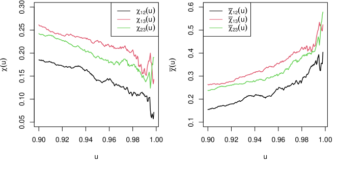
Figure 3: Empirical extremal dependence coefficients for data in C3

Figure 3 depicts the empirical estimates of $\chi(u)$ and $\bar{\chi}(u)$ for different pairs among $Y_{1},Y_{2},Y_{3}$. Although it is difficult to infer whether $\lim_{u\uparrow 1}\chi_{ij}(u)=0$ for $i,j=1,2,3,i\neq j$, i.e., whether $Y_{i}$ and $Y_{j}$ are asymptotically dependent or independent, we do observe that the extremal dependence among all pairs seems to be weak. This observation has led us to the selection of an asymptotically independent model for the estimation of the probability $p_{1}$; see more details in Section 3.2.2. To investigate the influence of the covariates season and atmosphere on the extremal dependence structure among $Y_{i}$s, we consider subsets of the data with different seasons and different atmosphere levels. The covariate season is discrete with only two possible values, S1 and S2, whilst the atmosphere is continuous. We thus categorize the covariate atmosphere into three classes, low, middle, and high, which correspond to the lowest $30\%$, the middle $40\%$, and the largest $30\%$ of the atmosphere respectively. The results in Table 2 indicate that the covariates do not seem to have significant influences on the extremal dependence structure. Hence, we choose to neglect the covariates and only use the observations of $Y$ to infer its extremal dependence structure across the three sites.

Table 2: Empirical extremal dependence coefficients for different seasons and atmosphere

	$\chi_{12}(0.975)$	$\chi_{13}(0.975)$	$\chi_{23}(0.975)$	$\bar{\chi}_{12}(0.975)$	$\bar{\chi}_{13}(0.975)$	$\bar{\chi}_{23}(0.975)$
Season S1	$0.11$	$0.24$	$0.17$	$0.26$	$0.44$	$0.35$
Season S2	$0.13$	$0.19$	$0.20$	$0.29$	$0.37$	$0.39$
Low atm.	$0.12$	$0.18$	$0.18$	$0.27$	$0.36$	$0.36$
Middle atm.	$0.09$	$0.21$	$0.16$	$0.20$	$0.40$	$0.33$
High atm.	$0.15$	$0.25$	$0.22$	$0.32$	$0.45$	$0.42$

3.2.2 Estimation of Probability $p_{1}$

Modeling dependence for multivariate extremes is a well-known challenging problem, especially in high dimensions [13]. Under the framework of multivariate regular variation, recent efforts to tackle this problem include the construction of sparse graphical models [12] and simple max-linear models [17, 6, 28]. In the latter case, one aims at finding a random vector, which follows a max-linear model, to approximate the data-generating regularly varying random vector by matching their tail pairwise dependence matrices.

Inspired by this idea, we here propose to find a Gaussian random vector to approximate an AI random vector by matching their matrices of pairwise coefficients of AI, $\bar{\chi}$. Note that we say a random vector $\mathbf{Y}\in\mathbb{R}^{d}$ is AI if all its marginal pairs are AI. For $\mathbf{Y}\in\mathbb{R}^{d}$, we denote its matrix of AI coefficients by $\bar{X}_{\mathbf{Y}}=(\bar{\chi}^{\mathbf{Y}}_{ij})_{d\times d},$ where $\bar{\chi}_{ij}$ denotes the coefficient of AI of $Y_{i}$ and $Y_{j}$. The matrix $\bar{X}_{\mathbf{Y}}$ clearly is symmetric, with diagonal elements being $1$ and non-diagonal elements between $0$ and $1$.

Now our goal is to find a Gaussian random vector $\mathbf{Z}\in\mathbb{R}^{d}$ such that its matrix of AI coefficients matches that of $\mathbf{Y}$, i.e., $\bar{X}_{\mathbf{Y}}=\bar{X}_{\mathbf{Z}}$. Assume that the matrix $\bar{X}_{\mathbf{Y}}$ is positive semi-definite, then one can construct the random vector $\mathbf{Z}$ as $\mathbf{Z}=L\mathbf{W}$, where $L$ is the lower triangular matrix associated with the Cholesky decomposition $\bar{X}_{\mathbf{Y}}=LL^{T}$, and $\mathbf{W}\in\mathbb{R}^{d}$ has independent standard normal components. This construction yields that the correlation matrix ${\rm Corr}(\mathbf{Z})$ is equal to $\bar{X}_{\mathbf{Y}}$, which further implies that $\bar{X}_{\mathbf{Y}}=\bar{X}_{\mathbf{Z}}$ since ${\rm Corr}(\mathbf{Z})=\bar{X}_{\mathbf{Z}}$ for Gaussian random vectors. Note that the positive semi-definiteness assumption of $\bar{X}_{\mathbf{Y}}$ seems to be weak. In the Gaussian case, it is equal to the correlation matrix and is typically assumed to be positive semi-definite. In general, the question whether the matrix $\bar{X}_{\mathbf{Y}}$ can only be positive semi-definite is not so straightforward to prove or disprove. Embrechts et al [11] has shown the positive semi-definiteness of the matrix of AD coefficients by establishing the link between this matrix and Bernoulli-compatible matrix, but the proof and results are not directly applicable to the matrix of AI coefficients.

In practice, one needs to estimate the matrix $\bar{X}_{\mathbf{Y}}$. Here we use the empirical estimator of $\bar{\chi}_{ij}^{\mathbf{Y}}(u)$, where $u$ is chosen to be $0.995$ since our sample size is as large as $21,000$. Our estimate of this matrix turns out to be positive definite. We thus use the methodology described above to obtain a Gaussian random vector $\mathbf{Z}$ with covariance matrix as our estimate of $\bar{X}_{\mathbf{Y}}$. Then the probability of interest, $p_{1}$, can be estimated by

$$\hat{p}_{1}=\mathbb{P}(Z_{1}>6,Z_{2}>6,Z_{3}>6)=2.14\cdot 10^{-5}.$$

3.2.3 Estimation of Probability $p_{2}$

To estimate the probability $p_{2}$, we use a different approach for estimating $p_{1}$ since the event of interest is not that $Y_{i},i=1,2,3$ are simultaneously extreme, but rather only $Y_{1},Y_{2}$ are extreme and $Y_{3}$ is smaller than its median. Note that

$$p_{2} =\mathbb{P}(Y_{1}>7,Y_{2}>7,Y_{3}<m)$$

$$=\mathbb{P}(Y_{1}>7,Y_{2}>7\mid Y_{3}<m)\mathbb{P}(Y_{3}<m)$$

$$=0.5\mathbb{P}(Y_{1}>7,Y_{2}>7\mid Y_{3}<m)$$

$$=0.5\mathbb{P}(\min(Y_{1},Y_{2})>7\mid Y_{3}<m)$$

since $m$ is the median of the marginal distribution of $Y_{3}$. Hence, estimating $p_{2}$ is equivalent to estimating the conditional probability $\mathbb{P}(\min(Y_{1},Y_{2})>7\mid Y_{3}<m)$, which boils down to estimating the tail of a random variable $\min(Y_{1},Y_{2})\mid Y_{3}<m$.

We here follow the standard approach in extreme value theory [5], and fit a generalized Pareto distribution (GPD) to high threshold exceedances of the observations of $\min(Y_{1},Y_{2})\mid Y_{3}<m$. The threshold is chosen to be the $95\%$ quantile of the data, after examining the parameter stability plot using the R package mev. The estimated scale and shape parameters of the GPD are respectively $0.63$ and $0.098$. By plugging in the estimated distribution of $\min(Y_{1},Y_{2})\mid Y_{3}<m$, we obtain the estimate of $p_{2}$ as $\hat{p}_{2}=3.81\cdot 10^{-5}$.

3.2.4 Results and Discussion

Our estimation for probabilities $p_{1}$ and $p_{2}$ both performs well compared with other teams. Here we have shown that in the presence of weak extremal dependence, a Gaussian copula can well describe the tail of data by matching their matrix of AI coefficients. This approach is computationally efficient and can be easily applied to high dimensions. An interesting future research question is to investigate whether the matrix of AI coefficients is positive semi-definite, which further determines whether one can always find a random vector $\mathbf{Z}$ such that its matrix of AI coefficients matches that of an arbitrarily given random vector $\mathbf{Y}$. Another interesting direction is to study how to incorporate covariates information in the degree of extremal dependence. This will allow one to construct non-stationary models for extremal dependence and capture more flexible dependence structures.

3.3 Multivariate Threshold Exceedances (Task C4)

3.3.1 Clustering of Pairwise Dependencies

Since the univariate marginal distributions are known to be standard Gumbel for each site, it is not necessary to transform the marginal distributions of the data, and we can turn our attention immediately to the multivariate interactions. In order to analyze the pairwise dependencies in the data, we consider the matrix of pairwise extremal correlation coefficients $\chi_{ij}$ (compare (7)) and the extremal variogram as introduced in [14]. The extremal variogram has proven to be very useful in the context of extremal graphical modelling, where the entries of a random vector are associated the node set $V$ of a graph, see Engelke and Hitz [12], Röttger et al [38] for further references and examples.

For a pre-asymptotic threshold $u\in(0,1)$, the extremal variogram rooted at node $m\in V$ is a matrix with entries $i,j$ defined as

$$\Gamma^{(m)}_{ij}(u) =\operatorname*{Var}(\log(1-F_{i}(Y_{i}))-\log(1-F_{j}(Y_{j}))\,\mid\,F_{m}(Y_{m})>1-u).$$ (9)

The limiting extremal variogram can be defined by considering $u\rightarrow 1$ in the equation above. Furthermore, the average over all $m\in V$ can be considered in order to define a single estimator, independent of a choice of $m$, see [14] for details.

These definitions can be turned into empirical estimators $\hat{\chi}_{ij}(u)$ and $\hat{\Gamma}_{ij}(u)$ by replacing the distribution function $F$ with an empirical version and computing the empirical variance in eq. 9. We computed the estimators $\hat{\chi}_{ij}(u)$ and $\hat{\Gamma}_{ij}(u)$ for all pairs $i,j$ and a range of threshold values $0.7\leq u\leq 1$. The result are shown in fig. 4.

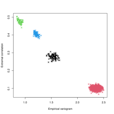
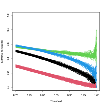
Figure 4: Extremal correlation and empirical variogram at threshold $u=0.9$ (left) and over a range of different thresholds (right). Four distinct clusters are clearly visible, stable for different values of $u$, and are color-coded according to the results of a hierarchical clustering algorithm.

From the scatter plot of $\hat{\chi}_{ij}(u)$ and $\hat{\Gamma}_{ij}(u)$ it is immediately visible that there seem to be four distinct clusters of pairwise interactions. The right-hand side of fig. 4 shows that these clusters are stable for different choices of $u$, even though two of them overlap for $u\leq 0.85$ and the lower two both seem to converge to zero for $u\rightarrow 1$. One approach to use this apparent symmetry for modelling are so-called colored graphical models, introduced for extreme value distributions in [38]. However, as we cannot assume an underlying tree structure we would require the parametric Hüsler–Reiss model, which seems unrealistic in this example. Instead, we discuss a more general approach that turned out to have better performance than the colored Hüsler–Reiss model.

3.3.2 Clustering of Sites

In order to obtain a partition of the sites themselves, rather than their pairwise interactions, we apply a hierarchical clustering method with the empirical extremal variogram at threshold $u=0.9$ as dissimilarity measure, akin to its use as distance in the minimum spanning tree procedure described in [14]. The resulting dendrogram and heatmap are shown in fig. 5, and clearly indicate the existence of five distinct clusters of sites. The pairwise dependencies inside each cluster are very homogeneous, belonging to a single cluster of values for each cluster of sites. Between sites from different clusters, the interaction is very weak, belonging to the large cluster of interaction values located near zero for the extremal correlation, and a large value for the extremal variogram.

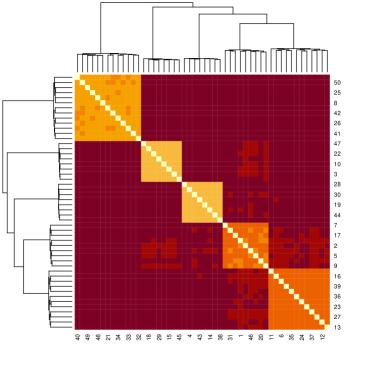
Figure 5: Hierarchical clustering of stations, using the empirical variogram $\hat{\Gamma}_{ij}$ at threshold $u=0.9$ as dissimilarity measure (left). Comparison of the empirical variogram between disconnected vertices for different values of $u$, compared to the theoretical value for asymptotically independent variables (right).

3.3.3 Independence Between Clusters

In the sequel we will model the probability of joint threshold exceedances assuming complete independence between sites from different clusters, yielding a simplified expression for the probability of a joint threshold exceedance of all sites:

$$\mathbb{P}(Y_{i}>s(i),i=1,\dots,50) =\prod_{j=1,\dots,5}\mathbb{P}(Y_{i}>s(i),i\in C_{j}),$$

where sites are indexed $1$ through $50$ and $s(i)$ denotes the relevant threshold for site $i$, depending on the considered scenario.

This assumption of asymptotic independence between clusters can be justified since the empirical extremal correlation $\hat{\chi}_{ij}$ for observations from different clusters steadily converges to zero. Furthermore, the classical covariance between such sites is near zero, as well, and the right-hand side of fig. 5 shows that the observed empirical extremal correlations (thin red lines) are very close to the theoretical values for independent variables (thick black line), which can be computed to be

$$\chi_{ij}(u) =\mathbb{P}(F_{i}(Y_{i})>u,F_{j}(Y_{j})>u)/(1-u)$$

$$=\mathbb{P}(F_{i}(Y_{i})>u)\mathbb{P}(F_{j}(Y_{j})>u)/(1-u)$$

$$=(1-u)^{2}/(1-u)$$

$$=(1-u).$$

Even though we decided to assume complete independence in the following computations, we note that there are some indications contradicting this assumption. For instance, in fig. 5, a number of empirical extremal correlation entries near $u\approx 1$ differ significantly from the theoretical value $1-u$, and the heatmap shows that sites in the fourth cluster (w.r.t. the order in which they are plotted) seem to have slightly stronger dependencies with sites from different clusters. However, considering how weak these indications are, we decided to continue with the independence assumption, leaving the modelling of inter-cluster dependencies for future research.

3.3.4 Analysis Inside Clusters

fig. 6 shows the number of joint exceedances in each cluster with respect to the two threshold combinations considered in the task. For clusters 2, 3 there is a significant number of observations in which all sites simultaneously exceed the thresholds. Using this, we model the simultaneous exceedance probabilities for these two clusters by simply considering their empirical counterparts

$$\hat{\mathbb{P}}(Y_{i}>s(i),i\in C_{j}) =\frac{\#\left\{t:Y_{t,i}>s(i),i\in C_{j}\right\}}{T},$$

for clusters $j=2,3$ and with $T$ denoting the total number of observations in the dataset.

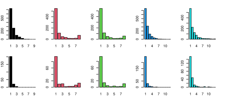
Figure 6: Simultaneous exceedances of the relevant threshold. X-axis of each plot indicates the (exact) number of observations that exceed the threshold at the same time. Y-axis indicates the number of occurrences of these exceedances. Top row is with respect to scenario (i), the bottom row is with respect to scenario (ii).

For the remaining three clusters there are no observed simultaneous exceedances, implying that their probabilities need to be extrapolated. Since the empirical values of summary statistics like the extremal correlation, extremal variogram, and multivariate extremal correlation [cf. 10] differ significantly between different clusters, we use a simple but flexible approach, described below.

In scenario (i), we define for each cluster index $j=1,\dots,5$ and threshold index $l=1,2$

$$M_{j,l}=\min_{i\in C_{j},s(i)=s_{l}}Y_{i},$$

yielding for each $j$ the equality

$$\mathbb{P}(Y_{i}>s(i),i\in C_{j}) =\mathbb{P}(M_{j,1}>s_{1},M_{j,2}>s_{2}).$$

In scenario (ii), all stations are compared to the same threshold, $s_{1}$, so the expressions above simplify to

$$M_{j} =\min_{i\in C_{j}}Y_{i},$$

$$\mathbb{P}(Y_{i}>s(i),i\in C_{j}) =\mathbb{P}(M_{j}>s_{1}).$$

This is a univariate threshold exceedance, which we model by fitting a generalized Pareto distribution (GPD) [cf. 5] to the tail $T_{j}$ of each $M_{j}$. More specifically, we consider a high intermediate threshold $p_{0}$, keep only observations exceeding the empirical quantile $\hat{Q}_{M_{j}}(p_{0})$, and, using maximum likelihood estimation, fit a GPD $T_{j,p_{0}}$ to these exceedances. The probability of an $s_{1}$-exceedance can then be estimated as

$$\hat{\mathbb{P}}(M_{j}>s_{1}) =\hat{\mathbb{P}}(M_{j}>\hat{Q}_{M_{j}}(p_{0}))\cdot\hat{\mathbb{P}}(M_{j}>s_{1}|M_{j}>\hat{Q}_{M_{j}}(p_{0}))$$

$$=(1-p_{0})\cdot\mathbb{P}(T_{j,p_{0}}>s_{1}),$$

which can be evaluated explicitly. In order to be more robust with respect to the choice of $p_{0}$, we averaged the final probability over a range of values $p_{0}\in(0.9,1.0)$.

Coming back to scenario (i), a bivariate exceedance probability needs to be evaluated:

$$\mathbb{P}(M_{j,1}>s_{1},M_{j,2}>s_{2}) =\mathbb{P}(M_{j,1}>s_{1})\mathbb{P}(M_{j,2}>s_{2}|M_{j,1}>s_{1}).$$

The first factor is again a univariate exceedance probability, which we estimate following the same procedure as above, fitting a GPD $S_{j,p_{0}}$ at intermediate threshold $p_{0}$. For the second factor, we have

$$1\geq\mathbb{P}(M_{j,2}>s_{2}|M_{j,1}>s_{1})\geq\mathbb{P}(M_{j,2}>s_{2}|M_{j,1}>s_{2})=\chi^{(j)}(Q_{M_{j,1}}(s_{2})),$$ (10)

where $\chi^{(j)}(u)$ denotes the extremal correlation between the two minima $M_{j,1}$ and $M_{j,2}$ at threshold $u$. The second inequality can be justified, since the event $\left\{M_{j,1}>s_{1}\right\}$ is a “more extreme” subset of $\left\{M_{j,1}>s_{2}\right\}$, and above we have observed positive extremal dependencies between all sites in each cluster. Since the estimated extremal correlations were rather large, we estimate the probability $\mathbb{P}(M_{j,2}>s_{2}|M_{j,1}>s_{1})$ by an estimate of its lower bound $\chi^{(j)}(Q_{M_{j,1}}(s_{2}))$.

Combining the above expressions, we get the final probability estimate

$$\hat{\mathbb{P}}(M_{j,1}>s_{1},M_{j,2}>s_{2}) =(1-p_{0})\cdot\mathbb{P}(S_{j,p_{0}}>s_{1})\cdot\hat{\chi}^{(j)},$$

which we again average over different thresholds $p_{0}$.

3.3.5 Final Estimates and Conclusion

Combining the steps above, the final estimates for the probabilities of interest are

$$\hat{p}_{1} =\prod_{j=2,3}\frac{\#\left\{t:Y_{t,i}>s(i),i\in C_{j}\right\}}{T}\prod_{j=1,4,5}(1-p_{0})\cdot\mathbb{P}(S_{j,p_{0}}>s_{1})\cdot\hat{\chi}^{(j)},$$

$$\hat{p}_{2} =\prod_{j=2,3}\frac{\#\left\{t:Y_{t,i}>s_{1},i\in C_{j}\right\}}{T}\prod_{j=1,4,5}(1-p_{0})\cdot\mathbb{P}(T_{j,p_{0}}>s_{1}).$$

These estimates are reasonably close to the true probabilities, underestimating them in both scenarios. The resulting log-scores, which were considered for the ranking, are very close to those of the other teams in the top five for this challenge.

We have demonstrated methods for identifying sparsity in the structure of pairwise interactions, and partitioning of sites accordingly. We applied a very general, but flexible framework to reduce the high-dimensional problem of joint threshold exceedance probabilities to a problem of univariate and bivariate exceedances, allowing the application of established peaks-over-threshold methods. However, especially in the case of mixed thresholds (scenario i), our estimates were somewhat rough and in future research, parametric models could likely be employed to obtain better estimates.

Declarations

Acknowledgments We thank Christian Rohrbeck, Emma Simpson and Jonathan Tawn for their efforts in organising the EVA 2023 data competition.

Availability of supporting data The data used in this study is described in detail in Rohrbeck et al [36].

Funding Authors were supported by Swiss National Science Foundation Eccellenza Grant 186858.

References

- \bibcommenthead
- Allouche et al [2024] Allouche M, Girard S, Gobet E (2024) Estimation of extreme quantiles from heavy-tailed distributions with neural networks. Stat and Comput 34(1):12
- Athey et al [2019] Athey S, Tibshirani J, Wager S (2019) Generalized random forests. Ann Stat 47(2):1148–1178
- Balkema and de Haan [1974] Balkema AA, de Haan L (1974) Residual Life Time at Great Age. Ann Probab 2(5):792 – 804
- Chavez-Demoulin and Davison [2005] Chavez-Demoulin V, Davison AC (2005) Generalized additive modelling of sample extremes. J R Stat Soc C 54(1):207–222
- Coles [2001] Coles S (2001) An Introduction to Statistical Modeling of Extreme Values. Springer, London
- Cooley and Thibaud [2019] Cooley D, Thibaud E (2019) Decompositions of dependence for high-dimensional extremes. Biometrika 106(3):587–604
- Daouia et al [2011] Daouia A, Gardes L, Girard S, et al (2011) Kernel estimators of extreme level curves. TEST 20(2):311–333
- Davison and Hinkley [1997] Davison AC, Hinkley DV (1997) Bootstrap Methods and their Application. Cambridge University Press, New York
- Davison et al [2003] Davison AC, Hinkley DV, Young GA (2003) Recent Developments in Bootstrap Methodology. Stat Sci 18(2):141–157
- de Haan and Zhou [2011] de Haan L, Zhou C (2011) Extreme residual dependence for random vectors and processes. Adv Appl Probab 43(1):217 – 242
- Embrechts et al [2016] Embrechts P, Hofert M, Wang R (2016) Bernoulli and tail-dependence compatibility. Ann Appl Probab 26(3):1636–1658
- Engelke and Hitz [2020] Engelke S, Hitz A (2020) Graphical models for extremes (with discussion). J R Stat Soc B 82:871–932
- Engelke and Ivanovs [2021] Engelke S, Ivanovs J (2021) Sparse structures for multivariate extremes. Annu Rev Statist Appl 8:241–270
- Engelke and Volgushev [2022] Engelke S, Volgushev S (2022) Structure Learning for Extremal Tree Models. J R Stat Soc B 84(5):2055–2087
- Fisher and Tippett [1928] Fisher RA, Tippett LHC (1928) Limiting forms of the frequency distribution of the largest or smallest member of a sample. Math Proc Camb Philos Soc 24(2):180–190
- Gardes and Stupfler [2019] Gardes L, Stupfler G (2019) An integrated functional Weissman estimator for conditional extreme quantiles. REVSTAT 17(1):109–144
- Gissbl and Klüppelberg [2018] Gissbl N, Klüppelberg C (2018) Max-linear models on directed acyclic graphs. Bernoulli 24:2693–2720
- Gnecco et al [2022] Gnecco N, Terefe EM, Engelke S (2022) Extremal Random Forests. ArXiv:2201.12865
- Gnedenko [1943] Gnedenko B (1943) Sur la distribution limite du terme maximum d’une série aléatoire. Ann of Math (2) 44:423–453
- Goodfellow et al [2016] Goodfellow I, Bengio Y, Courville A (2016) Deep Learning. MIT Press
- de Haan [1984] de Haan L (1984) A spectral representation for max-stable processes. Ann Probab 12(4):1194–1204
- de Haan and Zhou [2022] de Haan L, Zhou C (2022) Bootstrapping Extreme Value Estimators. J Am Stat Assoc
- Hastie et al [2015] Hastie T, Mazumder R, Lee JD, et al (2015) Matrix completion and low-rank SVD via fast alternating least squares. J Mach Learn Res 16(1):3367–3402
- Heffernan and Tawn [2004] Heffernan JE, Tawn JA (2004) A conditional approach for multivariate extreme values. J R Stat Soc B 66(3):497–546. With discussions and reply by the authors
- Hentschel et al [2022] Hentschel M, Engelke S, Segers J (2022) Statistical inference for Hüsler-Reiss graphical models through matrix completions. ArXiv:2210.14292
- Josse and Husson [2016] Josse J, Husson F (2016) missMDA: A Package for Handling Missing Values in Multivariate Data Analysis. J Stat Softw 70(1):1–31
- Kingma and Ba [2014] Kingma DP, Ba J (2014) Adam: A Method for Stochastic Optimization. 3rd Int Conf Learn Repres
- Kiriliouk and Zhou [2023] Kiriliouk A, Zhou C (2023) Estimating probabilities of multivariate failure sets based on pairwise tail dependence coefficeints. arXiv:2210.12618
- Koenker and Bassett [1978] Koenker R, Bassett GJr. (1978) Regression quantiles. Econometrica 46(1):33–50
- Koh [2023] Koh J (2023) Gradient boosting with extreme-value theory for wildfire prediction. Extremes 26:273–299
- Li and Wang [2019] Li D, Wang HJ (2019) Extreme Quantile Estimation for Autoregressive Models. J Bus Econ Stat 37(4):661–670
- Pasche and Engelke [2022] Pasche OC, Engelke S (2022) Neural Networks for Extreme Quantile Regression with an Application to Forecasting of Flood Risk. ArXiv:220807590
- Pickands [1975] Pickands JIII (1975) Statistical inference using extreme order statistics. Ann Statist 3:119–131
- Resnick [2008] Resnick SI (2008) Extreme values, regular variation and point processes. Springer, New York
- Richards and Huser [2022] Richards J, Huser R (2022) Regression modelling of spatiotemporal extreme U.S. wildfires via partially-interpretable neural networks. ArXiv:2208.07581
- Rohrbeck et al [2024+] Rohrbeck C, Simpson ES, Tawn JA (2024+) Editorial: EVA 2023 Data Challenge. Extremes
- Rootzén and Tajvidi [2006] Rootzén H, Tajvidi N (2006) Multivariate generalized Pareto distributions. Bernoulli 12(5):917–930
- Röttger et al [2023a] Röttger F, Coons JI, Grosdos A (2023a) Parametric and nonparametric symmetries in graphical models for extremes. ArXiv:2306.00703
- Röttger et al [2023b] Röttger F, Engelke S, Zwiernik P (2023b) Total positivity in multivariate extremes. Ann Statist 51(3):962–1004
- Smith [1999] Smith RL (1999) Bayesian and frequentist approaches to parametric predictive inference. In: Bernardo JM, Berger JO, Dawid AP, et al (eds) Bayesian Statistics 6. Oxford University Press, p 586–612
- Stekhoven and Bühlmann [2012] Stekhoven DJ, Bühlmann P (2012) MissForest — non-parametric missing value imputation for mixed-type data. Bioinformatics 28(1):112–118
- van Buuren and Groothuis-Oudshoorn [2011] van Buuren S, Groothuis-Oudshoorn K (2011) mice: Multivariate Imputation by Chained Equations in R. J Stat Softw 45(3):1–67
- Velthoen et al [2019] Velthoen J, Cai JJ, Jongbloed G, et al (2019) Improving precipitation forecasts using extreme quantile regression. Extremes 22(4):599–622
- Velthoen et al [2021] Velthoen J, Dombry C, Cai JJ, et al (2021) Gradient boosting for extreme quantile regression. ArXiv:2103.00808
- Wadsworth et al [2017] Wadsworth JL, Tawn JA, Davison AC, et al (2017) Modelling across extremal dependence classes. J R Stat Soc B 79(1):149–175
- Wan and Zhou [2023] Wan P, Zhou C (2023) Graphical lasso for extremes. ArXiv:2307.15004
- Wang et al [2012] Wang HJ, Li D, He X (2012) Estimation of High Conditional Quantiles for Heavy-Tailed Distributions. J Am Stat Assoc 107(500):1453–1464
- Youngman [2019] Youngman BD (2019) Generalized Additive Models for Exceedances of High Thresholds With an Application to Return Level Estimation for U.S. Wind Gusts. J Am Stat Assoc 114(528):1865–1879
- Zeder et al [2023] Zeder J, Sippel S, Pasche OC, et al (2023) The Effect of a Short Observational Record on the Statistics of Temperature Extremes. Geophys Res Lett 50(16)