A Simulation Preorder for Koopman-like Lifted Control Systems

Abstract

This paper introduces a simulation preorder among lifted systems, a generalization of finite-dimensional Koopman approximations (also known as approximate immersions) to systems with inputs. It is proved that this simulation relation implies the containment of both the open- and closed-loop behaviors. Optimization-based sufficient conditions are derived to verify the simulation relation in two special cases: i) a nonlinear (unlifted) system and an affine lifted system and, ii) two affine lifted systems. Numerical examples demonstrate the approach using backward reachable sets.

1 Introduction

Nonlinear systems are ubiquitous in nature and engineering, exhibiting complex dynamics that often defy traditional linear modeling approaches. The Koopman operator framework (Koopman, 1931), offers a promising alternative for understanding and analyzing nonlinear systems. This framework transforms a finite-dimensional nonlinear system into an infinite-dimensional linear system by viewing it through the lens of an infinite set of observable functions. While the Koopman operator provides a powerful theoretical foundation, its practical application is hindered by its infinite-dimensional nature. In addition, nonlinear systems generally do not admit an exact finite-dimensional linear representation (Liu et al., 2023).

To address these limitations, finite-dimensional Koopman approximations — also known as approximate immersions (Wang et al., 2023) — have emerged as a practical tool for modeling and analyzing nonlinear systems (Williams et al., 2015). These approaches lift the state into a higher — but finite — dimensional space through a lifting function. A linear dynamics in the lifted space is constructed to approximate the nonlinear dynamics. In (Sankaranarayanan, 2016), an autonomous system is abstracted into a linear (or algebraic) lifted system. This is used to infer invariants of the nonlinear system. In (Wang et al., 2023), an autonomous nonlinear system is lifted into a linear one to compute invariant sets. When such an immersion does not exist, a method to compute approximate immersions is proposed. Alternatively, extended dynamic mode decomposition (EDMD) has been proposed as a data-driven algorithm that computes a Koopman approximation using a dictionary of functions, which defines the lifting function (Williams et al., 2015). However, there is no guarantee that EDMD finds an accurate approximation when the subspace spanned by the dictionary is not invariant under the Koopman operator. To address this limitation, the Tunable Symmetric Subspace Decomposition algorithm is introduced in (Haseli and Cortés, 2023) to trade off between invariance and expressiveness by pruning the dictionary. While EDMD was originally developed for autonomous systems, generalizations to systems with inputs have been developed (Proctor et al., 2018). For example, in (Korda and Mezić, 2018) model predictive control on a linear lifted system is used to control a nonlinear system. However, one major challenge with EDMD is the selection of the lifting function, which can significantly impact the accuracy and applicability of the approximation. In (Colbrook, 2023, Sec. 6.4), this is considered “one of the most significant open problems” in the finite-dimensional Koopman framework.

In this work, we develop a theoretical framework to tackle this challenge. Inspired by the success of simulation relations to build a simpler (e.g., discrete) representation of a nonlinear system (Girard and Pappas, 2007; Tabuada, 2009; Zamani et al., 2011; Liu and Ozay, 2016), we propose a new notion of simulation between lifted control systems.

Contribution: We introduce the concept of a lifted system as a natural generalization of finite-dimensional Koopman models to lifted nonlinear and set-valued dynamical systems with inputs. Then, a notion of simulation between lifted systems is defined. It is proved that when one lifted system simulates another, the open- (resp. closed-) loop behavior of the former is contained within the open- (resp. closed-) loop behavior of the latter. It follows that if a simulating lifted system satisfies some given specifications for a given controller, then the same controller can be used to satisfy the same specifications for the simulated system. Finally, we derive optimization-based sufficient conditions to (i) find an affine lifted system that simulates a nonlinear polynomial system, and (ii) verify if one affine lifted system simulates another. These results enable us to compare different lifting functions and alternative lifted systems in terms of their usefulness in control design. Our framework is illustrated on numerical examples through the computation of constrained backward reachable sets.

Notation: For two sets $\mathcal{X}$ and $\mathcal{Y}$, $\mathcal{Y}^{\mathcal{X}}$ is the set of functions $f:\mathcal{X}\rightarrow\mathcal{Y}$ from $\mathcal{X}$ to $\mathcal{Y}$. $f:\mathcal{X}\rightrightarrows\mathcal{Y}$ is a set-valued map from $\mathcal{X}$ to $\mathcal{Y}$, i.e., it is a function from $\mathcal{X}$ to $2^{\mathcal{Y}}$. For a subset $X\subseteq\mathcal{X}$, the image of $X$ under a function $f:\mathcal{X}\rightarrow\mathcal{Y}$ is the set $f(X)\coloneqq\{f(x)\in\mathcal{Y}\mid x\in X\}$. For a subset $Y\subseteq\mathcal{Y}$, the pre-image of $Y$ under $f$ is the set $f^{-1}[Y]\coloneqq\{x\in\mathcal{X}\mid f(x)\in Y\}$. Intervals in $\mathbb{R}$ are denoted $[a,b]$ and discrete intervals are denoted $[a;b]\coloneqq[a,b]\cap\mathbb{Z}$. For a set $\mathcal{A}$, $\mathcal{A}^{*}\coloneqq\bigcup_{T\in\mathbb{Z}_{+}}\mathcal{A}^{[0;T[}$ is the set of finite signals with values in $\mathcal{A}$, while $\mathcal{A}^{\infty}\coloneqq\mathcal{A}^{*}\cup\mathcal{A}^{[0;\infty[}$ is the set of finite and infinite signals with values in $\mathcal{A}$. The Minkowski sum of two sets $\mathcal{X}$ and $\mathcal{Y}$ is denoted $\mathcal{X}\oplus\mathcal{Y}$, and the $n$-th Minkowski power of $\mathcal{X}$ is denoted $\mathcal{X}^{n}$. The identity matrix in $\mathbb{R}^{n\times n}$ is denoted $I_{n}$ (or $I$ when the dimension is clear), and the zero matrix in $\mathbb{R}^{m\times n}$ is denoted $0_{m\times n}$ (or $0$ when the dimension is clear).

2 Lifted Systems and Simulations

We consider a discrete-time control system with set valued dynamics

$$x(t+1)\in f_{\mathcal{X}}(x(t),u(t)),$$ (1)

with state $x(t)\in\mathcal{X}\subseteq\mathbb{R}^{n_{\mathcal{X}}}$, and input $u(t)\in\mathcal{U}$. We are interested in finding controllers that satisfy some given specifications (e.g., reach-avoid constraints). To this end, we consider a lifted system, e.g., for which the control design might be easier.

Definition 1

A lifted system is a tuple $\mathsf{LifSys}_{\mathcal{Y}}=\\ (\mathcal{X},\mathcal{U},\psi_{\mathcal{Y}},f_{\mathcal{Y}},g_{\mathcal{Y}})$ with:

• $\mathcal{X}\subseteq\mathbb{R}^{n_{\mathcal{X}}}$ a set

• $\mathcal{U}$ an input set

• $\psi_{\mathcal{Y}}:\mathbb{R}^{n_{\mathcal{X}}}\rightarrow\mathbb{R}^{n_{\mathcal{Y}}}$ a lifting function

• $f_{\mathcal{Y}}:\mathbb{R}^{n_{\mathcal{Y}}}\times\mathcal{U}\rightrightarrows\mathbb{R}^{n_{\mathcal{Y}}}$ a dynamics

• $g_{\mathcal{Y}}:\mathbb{R}^{n_{\mathcal{Y}}}\rightarrow\mathbb{R}^{n_{\mathcal{X}}}$ an output map such that for all $x\in\mathbb{R}^{n_{\mathcal{X}}}$, $g_{\mathcal{Y}}(\psi_{\mathcal{Y}}(x))=x$.

The dimension of the lifted system is $n_{\mathcal{Y}}$. The lifted system is said to be affine if $f_{\mathcal{Y}}(y,u)=A_{\mathcal{Y}}y+B_{\mathcal{Y}}u\oplus W_{\mathcal{Y}}$ and $g_{\mathcal{Y}}(y)=C_{\mathcal{Y}}y$ for some matrices $A_{\mathcal{Y}}$, $B_{\mathcal{Y}}$, $C_{\mathcal{Y}}$, and some (possibly unbounded) polyhedra $W_{\mathcal{Y}}$.

An unlifted system is a lifted system whose dimension is $n_{\mathcal{X}}$ and lifting function and output maps are the identity. An unlifted system can be identified to the system (1).

Since the output map $g_{\mathcal{Y}}$ is a left inverse of the lifting function $\psi_{\mathcal{Y}}$, it follows that $\psi_{\mathcal{Y}}$ is injective and $g_{\mathcal{Y}}$ is surjective.

We use the following notation: for a lifted system $\mathsf{LifSys}_{\mathcal{A}}$, its lifting function, dynamics, output map and dimension are denoted $\psi_{\mathcal{A}}$, $f_{\mathcal{A}}$, $g_{\mathcal{A}}$ and $n_{\mathcal{A}}$, respectively. Similarly, if the lifted system is affine, the quantities $A_{\mathcal{A}}$, $B_{\mathcal{A}}$, $C_{\mathcal{A}}$, and $W_{\mathcal{A}}$ describe its dynamics as in Definition 1.

From a practical perspective, our goal is to abstract a nonlinear unlifted system into an affine lifted system. In addition, we want to be able to compare two affine lifted systems.

Definition 2

A tuple $(x,u,y)\in\mathcal{X}^{[0;T[}\times\mathcal{U}^{[0;T[}\times(\mathbb{R}^{n_{\mathcal{Y}}})^{[0;T[}$ is a solution of the lifted system $\mathsf{LifSys}_{\mathcal{Y}}$ (on $[0;T[$) if $T\in\mathbb{Z}_{+}\cup\{\infty\}$ and

$$y(0) =\psi_{\mathcal{Y}}(x(0))$$

$$y(t+1) \in f_{\mathcal{Y}}(y(t),u(t))\ \forall t\in[0;T-1[$$

$$x(t) =g_{\mathcal{Y}}(y(t))\ \forall t\in[0;T[.$$

A solution is maximal when either (i) $T=\infty$, or (ii) $T<\infty$ and $f_{\mathcal{Y}}(y(T-1),u(T-1))=\emptyset$, or (iii) $T<\infty$ and $g_{\mathcal{Y}}(f_{\mathcal{Y}}(y(T-1),u(T-1)))\nsubseteq\mathcal{X}$.

The state of the lifted system $\mathsf{LifSys}_{\mathcal{Y}}$ refers to $y(t)$ and its output refers to $x(t)$. The set of initial states is implicitly given by $y(0)\in\psi_{\mathcal{Y}}(\mathcal{X})$.

Note that the condition $x(t)\in\mathcal{X}$ is not necessarily satisfied by $x(t)=g_{\mathcal{Y}}(y(t))$ since $y(t)\in\mathbb{R}^{n_{\mathcal{Y}}}$. For that reason, we define the domain of the lifted system $\mathsf{LifSys}_{\mathcal{Y}}$ as the set of states $y$ that give an output in $\mathcal{X}$. It is written $\mathcal{D}_{\mathcal{Y}}\coloneqq g_{\mathcal{Y}}^{-1}[\mathcal{X}]=\{y\in\mathbb{R}^{n_{\mathcal{Y}}}\mid g_{\mathcal{Y}}(y)\in\mathcal{X}\}$.

The case (ii) for a solution to be maximal happens when the solution can not be extended. The case (iii) indicates that the state may leave the domain $\mathcal{D}_{\mathcal{Y}}$, i.e., $f_{\mathcal{Y}}(y(T-1),u(T-1))\nsubseteq\mathcal{D}_{\mathcal{Y}}$.

We define the behavior of a lifted system next.

Definition 3

The behavior of a lifted system $\mathsf{LifSys}_{\mathcal{Y}}$ is the set

$$\{(x,u)\mid\exists y,T:(x,u,y)\text{ is a solution of }\mathsf{LifSys}_{\mathcal{Y}}\text{ on }[0;T[$$

$$\text{ that is maximal.}\},$$

and is denoted $\mathcal{B}[\mathsf{LifSys}_{\mathcal{Y}}]$. The closed-loop behavior of a lifted system $\mathsf{LifSys}_{\mathcal{Y}}$ under a policy $\pi:\mathcal{X}^{*}\rightarrow\mathcal{U}$ is the set

$$\{(x,u)\in\mathcal{B}[\mathsf{LifSys}_{\mathcal{Y}}]\mid u(t)=\pi(x(0),\dots,x(t))\ \forall t\in[0;T[\},$$

and is denoted $\mathcal{B}_{\pi}[\mathsf{LifSys}_{\mathcal{Y}}]$.

Note that the feedback policy $\pi$ is a function of the previous outputs $x(t)$ and not a function of the previous states $y(t)$. This allows us to implement policies designed for the lifted system on the unlifted one, and compare closed-loop behaviors.

Let us define the notion of specification over $\mathcal{X}\times\mathcal{U}$, and the notion of specification satisfaction.

Definition 4

A specification over $\mathcal{X}\times\mathcal{U}$ is a set $S\subseteq(\mathcal{X}\times\mathcal{U})^{\infty}$. We say that the lifted system $\mathsf{LifSys}$ under the policy $\pi:\mathcal{X}^{*}\rightarrow\mathcal{U}$ satisfies the specification $S$ if the closed-loop behavior of the lifted system $\mathsf{LifSys}$ under the policy $\pi$ is included in the specifications, i.e., $\mathcal{B}_{\pi}[\mathsf{LifSys}]\subseteq S$. In that case, we write $\mathsf{LifSys}\models_{\pi}S$.

2.1 Simulation between lifted systems

In this section, we introduce the notion of simulation between lifted systems. Then, we prove that this relation implies the containment of closed- and open-loop behaviors of the lifted systems.

Definition 5

Given two lifted systems $\mathsf{LifSys}_{\mathcal{Y}}$ and $\mathsf{LifSys}_{\mathcal{Z}}$, we say that $\mathsf{LifSys}_{\mathcal{Z}}$ simulates $\mathsf{LifSys}_{\mathcal{Y}}$ (or that $\mathsf{LifSys}_{\mathcal{Y}}$ refines $\mathsf{LifSys}_{\mathcal{Z}}$), if there exists a set-valued function (called refinement map) $\rho:\mathbb{R}^{n_{\mathcal{Z}}}\rightrightarrows\mathbb{R}^{n_{\mathcal{Y}}}$ such that

$$\forall x\in\mathcal{X}: \ \psi_{\mathcal{Y}}(x)\in\rho(\psi_{\mathcal{Z}}(x))$$ (2a)

$$\forall(z,u)\in\mathcal{D}_{\mathcal{Z}}\times\mathcal{U}: \ f_{\mathcal{Y}}(\rho(z),u)\subseteq\rho(f_{\mathcal{Z}}(z,u))$$ (2b)

$$\forall z\in\mathbb{R}^{n_{\mathcal{Z}}}: \ g_{\mathcal{Y}}(\rho(z))\subseteq\{g_{\mathcal{Z}}(z)\}$$ (2c)

$$\forall(z,u)\in\mathcal{D}_{\mathcal{Z}}\times\mathcal{U},\forall y\in \rho(z):\ f_{\mathcal{Y}}(y,u)=\emptyset\Rightarrow f_{\mathcal{Z}}(z,u)=\emptyset.$$ (2d)

In that case, we write $\mathsf{LifSys}_{\mathcal{Y}}\preceq\mathsf{LifSys}_{\mathcal{Z}}$ (or $\mathsf{LifSys}_{\mathcal{Y}}\preceq_{\rho}\mathsf{LifSys}_{\mathcal{Z}}$ to make the refinement map explicit).

Since $g_{\mathcal{A}}$ is the left inverse of $\psi_{\mathcal{A}}$ for $\mathcal{A}\in\{\mathcal{Y},\mathcal{Z}\}$, condition (2a) ensures that any pair of initial states $y(0)$ and $z(0)$ of $\mathsf{LifSys}_{\mathcal{Y}}$ and $\mathsf{LifSys}_{\mathcal{Z}}$ that give the same output, i.e., $g_{\mathcal{Y}}(y(0))=g_{\mathcal{Z}}(z(0))=x(0)$ are related through $\rho$, i.e., $y(0)\in\rho(z(0))$.

Condition (2b) ensures that if $y$ and $z$ are related through $\rho$, i.e., $y\in\rho(z)$, and if $z$ is in the domain $\mathcal{D}_{\mathcal{Z}}$, then, their successors $y^{+}$ and $z^{+}$ will be related in the same way, i.e., $y^{+}\in\rho(z^{+})$. This condition can be rewritten using quantifiers as

$$\forall(z,u)\in\mathcal{D}_{\mathcal{Z}}\times\mathcal{U},\forall y\in\rho(z),\forall y^{+}\in f_{\mathcal{Y}}(y,u),$$

$$\exists z^{+}\in f_{\mathcal{Z}}(z,u)\text{ s.t. }y^{+}\in\rho(z^{+}).$$

This condition differs from the one used for simulation relations (Tabuada, 2009, Def. 4.7. Cond. 3.) in that simulation relations consider two different inputs $u_{\mathcal{Z}}$ and $u_{\mathcal{Y}}$. It also differs from the condition used for feedback refinement (Reissig et al., 2016, Def. V.2 (ii)) in that for feedback refinement, the quantifier over $z^{+}$ is $\forall z^{+}$ instead of $\exists z^{+}$.

Condition (2c) states that if $y$ and $z$ are related through $\rho$, then they must have the same output, i.e., $g_{\mathcal{Y}}(y)=g_{\mathcal{Z}}(z)$. A similar condition can be found in (Majumdar et al., 2020, Def. 3.1, (A3)). Condition (2c) implies that the domains of the two lifted systems satisfy

$$\rho(\mathcal{D}_{\mathcal{Z}})\subseteq\mathcal{D}_{\mathcal{Y}}.$$ (3)

Indeed, if $z\in\mathcal{D}_{\mathcal{Z}}$, i.e., $g_{\mathcal{Z}}(z)\in\mathcal{X}$, then $g_{\mathcal{Y}}(\rho(z))\subseteq\{g_{\mathcal{Z}}(z)\}\subseteq\mathcal{X}$, which is $\rho(z)\subseteq\mathcal{D}_{\mathcal{Y}}$. Informally, (3) can be interpreted as the domain $\mathcal{D}_{\mathcal{Y}}$ being “not smaller” than the domain $\mathcal{D}_{\mathcal{Z}}$.

Finally, (2d) states that if $z$ is in the domain and $y$ is related to $z$, then if $y$ is blocking for an input $u$, then $z$ must be blocking for the same $u$. A similar condition is considered in the context of feedback refinement for output feedback control (Reissig et al., 2016, Def. V.2 (i)). Note that if the dynamics $f_{\mathcal{Y}}(y,u)$ is non-blocking, then (2d) trivially holds.

Theorem 1

The relation $\preceq$ is a preorder, i.e., given three lifted systems $\mathsf{LifSys}_{i}$ for $i=1,2,3$, the following transitivity property holds: $\mathsf{LifSys}_{1}\preceq_{\rho_{1\leftarrow 2}}\mathsf{LifSys}_{2}\preceq_{\rho_{2\leftarrow 3}}\mathsf{LifSys}_{3}$ implies $\mathsf{LifSys}_{1}\preceq_{\rho_{1\leftarrow 2}\circ\rho_{2\leftarrow 3}}\mathsf{LifSys}_{3}$; and the following reflexivity property holds: $\mathsf{LifSys}_{i}\preceq_{I}\mathsf{LifSys}_{i}$.

The proof of the reflexivity is straightforward. To prove transitivity, let us denote $\rho_{1\leftarrow 3}\coloneqq\rho_{1\leftarrow 2}\circ\rho_{2\leftarrow 3}$ and write $\eqref{eq:order}_{i\leftarrow j}$ to refer to the equations (2) for $\mathsf{LifSys}_{i}\preceq_{\rho_{i\leftarrow j}}\mathsf{LifSys}_{j}$. Given $\eqref{eq:order}_{1\leftarrow 2}$ and $\eqref{eq:order}_{2\leftarrow 3}$, we need to prove $\eqref{eq:order}_{1\leftarrow 3}$.

For $\eqref{eq:order:psi}_{1\leftarrow 3}$: Let $x\in\mathcal{X}$. Using $\eqref{eq:order:psi}_{1\leftarrow 2}$ and $\eqref{eq:order:psi}_{2\leftarrow 3}$, we have $\psi_{1}(x)\in\rho_{1\leftarrow 2}(\psi_{2}(x))\subseteq\rho_{1\leftarrow 2}(\rho_{2\leftarrow 3}(\psi_{3}(x)))$, which proves $\eqref{eq:order:psi}_{1\leftarrow 3}$.

For $\eqref{eq:order:dyn}_{1\leftarrow 3}$: Let $(z,u)\in\mathcal{D}_{3}\times\mathcal{U}$. Using $\eqref{eq:order:dyn}_{2\leftarrow 3}$, $f_{2}(\rho_{2\leftarrow 3}(z),u)\subseteq\rho_{2\leftarrow 3}(f_{3}(z,u))$ and then $\rho_{1\leftarrow 2}(f_{2}(\rho_{2\leftarrow 3}(z),\\ u))\subseteq\rho_{1\leftarrow 2}(\rho_{2\leftarrow 3}(f_{3}(z,u)))$. On the other hand, using (3), $\rho_{2\leftarrow 3}(z)\subseteq\mathcal{D}_{2}$, and $\eqref{eq:order:dyn}_{1\leftarrow 2}$ gives $f_{1}(\rho_{1\leftarrow 2}(\rho_{2\leftarrow 3}(z)),u)\subseteq\rho_{1\leftarrow 2}(f_{2}(\rho_{2\leftarrow 3}(z),u))$. We have shown that the right hand side is included in $\rho_{1\leftarrow 3}(f_{3}(z,u))$, so $f_{1}(\rho_{1\leftarrow 3}(z),u)\subseteq\rho_{1\leftarrow 3}(f_{3}(z,u))$, which concludes the proof of $\eqref{eq:order:dyn}_{1\leftarrow 3}$.

For $\eqref{eq:order:output}_{1\leftarrow 3}$: Let $z\in\mathbb{R}^{n_{3}}$. From $\eqref{eq:order:output}_{1\leftarrow 2}$, $g_{1}(\rho_{1\leftarrow 2}(\rho_{2\leftarrow 3}(z)))\\ \subseteq g_{2}(\rho_{2\leftarrow 3}(z))$ and from $\eqref{eq:order:output}_{2\leftarrow 3}$, the right hand side is included in $\{g_{3}(z)\}$, which shows $\eqref{eq:order:output}_{1\leftarrow 3}$ holds.

For $\eqref{eq:order:block}_{1\leftarrow 3}$: Let $(z_{3},u)\in\mathcal{D}_{3}\times\mathcal{U}$ and let $z_{1}\in\rho_{1\leftarrow 2}(\rho_{2\leftarrow 3}(z_{3}))$. Then, there exists $z_{2}\in\rho_{2\leftarrow 3}(z_{3})$ such that $z_{1}\in\rho_{1\leftarrow 2}(z_{2})$. It follows from (3) that $z_{2}\in\mathcal{D}_{2}$. Then, $\eqref{eq:order:block}_{1\leftarrow 2}$ and $\eqref{eq:order:block}_{2\leftarrow 3}$ imply that if $f_{1}(z_{1},u)=\emptyset$, then $f_{2}(z_{2},u)=\emptyset$, and then $f_{3}(z_{3},u)=\emptyset$; proving $\eqref{eq:order:block}_{1\leftarrow 3}$.∎

The next theorem states that the open-loop behavior of a lifted system is included in the behavior of its simulation.

Theorem 2

Given two lifted systems $\mathsf{LifSys}_{\mathcal{Y}}$ and $\mathsf{LifSys}_{\mathcal{Z}}$, if $\mathsf{LifSys}_{\mathcal{Y}}$ refines $\mathsf{LifSys}_{\mathcal{Z}}$, then the behavior of $\mathsf{LifSys}_{\mathcal{Y}}$ is included in the behavior of $\mathsf{LifSys}_{\mathcal{Z}}$, i.e., $\mathsf{LifSys}_{\mathcal{Y}}\preceq\mathsf{LifSys}_{\mathcal{Z}}$ implies $\mathcal{B}[\mathsf{LifSys}_{\mathcal{Y}}]\subseteq\mathcal{B}[\mathsf{LifSys}_{\mathcal{Z}}]$.

Assume that $\mathsf{LifSys}_{\mathcal{Y}}\preceq_{\rho}\mathsf{LifSys}_{\mathcal{Z}}$ and let $(x,u)\in\mathcal{B}[\mathsf{LifSys}_{\mathcal{Y}}]$. Then, there exists $y$ and $T$ such that $(x,u,y)$ is a maximal solution of $\mathsf{LifSys}_{\mathcal{Y}}$ on $[0;T[$. We need to show that there exists $z$ such that $(x,u,z)$ is a maximal solution of $\mathsf{LifSys}_{\mathcal{Z}}$ on $[0;T[$.

First, let us prove the following statement (S): for all $t\in[0;T-1[$, if there exists a $z\in\mathbb{R}^{n_{\mathcal{Z}}}$ such that $y(t)\in\rho(z)$ and $g_{\mathcal{Z}}(z)=x(t)$, then there exists $z^{+}\in f_{\mathcal{Z}}(z,u(t))$ such that $y(t+1)\in\rho(z^{+})$ and $g_{\mathcal{Z}}(z^{+})=x(t+1)$. To prove (S), note that $g_{\mathcal{Z}}(z)=x(t)\in\mathcal{X}$ implies $z\in\mathcal{D}_{\mathcal{Z}}$. Then, using (2b), one can write

$$y(t+1)\in f_{\mathcal{Y}}(y(t),u(t))\subseteq f_{\mathcal{Y}}(\rho(z),u(t))\subseteq\rho(f_{\mathcal{Z}}(z,u(t))),$$

which implies that there exists $z^{+}\in f_{\mathcal{Z}}(z,u(t))$ such that $y(t+1)\in\rho(z^{+})$. Then, using (2c), one can write

$$x(t+1)=g_{\mathcal{Y}}(y(t+1))\in g_{\mathcal{Y}}(\rho(z^{+}))\subseteq\{g_{\mathcal{Z}}(z^{+})\},$$

and $g_{\mathcal{Z}}(z^{+})=x(t+1)$. This concludes the proof of (S).

Because $z(0)\coloneqq\psi_{\mathcal{Z}}(x(0))$ satisfies $y(0)\in\rho(z(0))$ (thanks to (2a)) and $g_{\mathcal{Z}}(z(0))=x(0)$ (because $g_{\mathcal{Z}}$ is a left inverse of $\psi_{\mathcal{Z}}$), it follows recursively from (S) that there exists a sequence $z\in(\mathbb{R}^{n_{\mathcal{Z}}})^{[0;T[}$ such that $(x,u,z)$ is a solution of $\mathsf{LifSys}_{\mathcal{Z}}$ on $[0;T[$ and $y(t)\in\rho(z(t))$ for all $t\in[0;T[$.

It remains to prove that the solution $(x,u,z)$ is maximal. Since $(x,u,y)$ is maximal, either (i) $T=\infty$, and $(x,u,z)$ is maximal; or (ii) $T<\infty$ and $f_{\mathcal{Y}}(y(T-1),u(T-1))=\emptyset$. Since $y(T-1)\in\rho(z(T-1))$, (2d) implies $f_{\mathcal{Z}}(z(T-1),u(T-1))=\emptyset$ and $(x,u,z)$ is maximal; or (iii) $T<\infty$ and $g_{\mathcal{Y}}(f_{\mathcal{Y}}(y(T-1),u(T-1)))\nsubseteq\mathcal{X}$. It follows from $y(T-1)\in\rho(z(T-1))$ and (2b) that

$$f_{\mathcal{Y}}(y(T-1),u(T-1)) \subseteq f_{\mathcal{Y}}(\rho(z(T-1)),u(T-1))$$

$$\subseteq\rho(f_{\mathcal{Z}}(z(T-1),u(T-1))).$$

Then, using (2c),

$$g_{\mathcal{Y}}(f_{\mathcal{Y}}(y(T-1),u(T -1)))$$

$$\subseteq g_{\mathcal{Y}}(\rho(f_{\mathcal{Z}}(z(T-1),u(T-1))))$$

$$\subseteq g_{\mathcal{Z}}(f_{\mathcal{Z}}(z(T-1),u(T-1))),$$

which implies $g_{\mathcal{Z}}(f_{\mathcal{Z}}(z(T-1),u(T-1)))\nsubseteq\mathcal{X}$, and $(x,u,z)$ is maximal. This concludes the proof. ∎

A consequence of Theorem 2 is the inclusion of closed-loop behaviors.

Corollary 3

Given two lifted systems $\mathsf{LifSys}_{\mathcal{Y}}$, $\mathsf{LifSys}_{\mathcal{Z}}$, and a policy $\pi:\mathcal{X}^{*}\rightarrow\mathcal{U}$, if $\mathsf{LifSys}_{\mathcal{Y}}$ refines $\mathsf{LifSys}_{\mathcal{Z}}$, then the closed-loop behavior of $\mathsf{LifSys}_{\mathcal{Y}}$ under $\pi$ is included in the closed-loop behavior of $\mathsf{LifSys}_{\mathcal{Z}}$ under $\pi$, i.e., $\mathsf{LifSys}_{\mathcal{Y}}\preceq\mathsf{LifSys}_{\mathcal{Z}}$ implies $\mathcal{B}_{\pi}[\mathsf{LifSys}_{\mathcal{Y}}]\subseteq\mathcal{B}_{\pi}[\mathsf{LifSys}_{\mathcal{Z}}]$.

For a given policy $\pi:\mathcal{X}^{*}\rightarrow\mathcal{U}$, define the set

$$\Pi\coloneqq\bigcup_{T\in\mathbb{Z}_{+}\cup\{\infty\}}\{ (x,u)\in\mathcal{X}^{[0;T[}\times\mathcal{U}^{[0;T[}\mid$$

$$u(t)=\pi(x(0),\dots,x(t)),\ \forall t\in[0;T[\}.$$

By definition of the closed loop behavior, $\mathcal{B}_{\pi}[\mathsf{LifSys}_{\mathcal{A}}]=\mathcal{B}[\mathsf{LifSys}_{\mathcal{A}}]\cap\Pi$ for $\mathcal{A}\in\{\mathcal{Y},\mathcal{Z}\}$. By Theorem 2, $\mathsf{LifSys}_{\mathcal{Y}}\preceq\mathsf{LifSys}_{\mathcal{Z}}$ implies $\mathcal{B}[\mathsf{LifSys}_{\mathcal{Y}}]\subseteq\mathcal{B}[\mathsf{LifSys}_{\mathcal{Z}}]$. Then, $\mathcal{B}[\mathsf{LifSys}_{\mathcal{Y}}]\cap\Pi\subseteq\mathcal{B}[\mathsf{LifSys}_{\mathcal{Z}}]\cap\Pi$, concluding the proof.∎

A direct consequence of Corollary 3 is that if an abstract lifted system under a policy satisfies some specification, then the concrete system under the same policy satisfies this specification as well.

Corollary 4

Given two lifted systems $\mathsf{LifSys}_{\mathcal{Y}}$, $\mathsf{LifSys}_{\mathcal{Z}}$, a policy $\pi:\mathcal{X}^{*}\rightarrow\mathcal{U}$, and a specification $S$ over $\mathcal{X}\times\mathcal{U}$, if $\mathsf{LifSys}_{\mathcal{Y}}$ refines $\mathsf{LifSys}_{\mathcal{Z}}$, and if $\mathsf{LifSys}_{\mathcal{Z}}$ satisfies the specification $S$ under the policy $\pi$, then $\mathsf{LifSys}_{\mathcal{Y}}$ satisfies the same specification $S$ under the same policy $\pi$, i.e., $\mathsf{LifSys}_{\mathcal{Y}}\preceq\mathsf{LifSys}_{\mathcal{Z}}\models_{\pi}S$ implies $\mathsf{LifSys}_{\mathcal{Y}}\models_{\pi}S$.

Informally, if $\mathsf{LifSys}_{\mathcal{Y}}$ and $\mathsf{LifSys}_{\mathcal{Z}}$ are two abstractions of the same concrete system of interest $\mathsf{LifSys}_{\mathcal{X}}$, and if $\mathsf{LifSys}_{\mathcal{Y}}\preceq\mathsf{LifSys}_{\mathcal{Z}}$, then $\mathsf{LifSys}_{\mathcal{Y}}$ is a “not worse” representation of $\mathsf{LifSys}_{\mathcal{X}}$ than $\mathsf{LifSys}_{\mathcal{Z}}$ in terms of specification satisfaction.

2.2 Simulating unlifted systems

In this Section, we focus on the special case where the simulated system is unlifted. The next theorem gives a sufficient condition to simulate an unlifted system.

Theorem 5

Given an unlifted system $\mathsf{LifSys}_{\mathcal{X}}$ and a lifted system $\mathsf{LifSys}_{\mathcal{Z}}$, $\mathsf{LifSys}_{\mathcal{Z}}$ simulates $\mathsf{LifSys}_{\mathcal{X}}$ with refinement map $\psi_{\mathcal{Z}}^{-1}$, i.e., $\mathsf{LifSys}_{\mathcal{X}}\preceq_{\psi^{-1}_{\mathcal{Z}}}\mathsf{LifSys}_{\mathcal{Z}}$, if and only if $\forall(x,u)\in\mathcal{X}\times\mathcal{U}$:

$$\psi_{\mathcal{Z}}(f_{\mathcal{X}}(x,u)) \subseteq f_{\mathcal{Z}}(\psi_{\mathcal{Z}}(x),u),$$ (4a)

$$f_{\mathcal{X}}(x,u)=\emptyset \Rightarrow f_{\mathcal{Z}}(\psi_{\mathcal{Z}}(x),u)=\emptyset.$$ (4b)

First, (2a) reduces to $x\in\psi_{\mathcal{Z}}^{-1}[\psi_{\mathcal{Z}}(x)]$ which holds trivially. Similarly, (2c) reduces to $\psi_{\mathcal{Z}}^{-1}[z]\subseteq\{g_{\mathcal{Z}}(z)\}$ which holds since $g_{\mathcal{Z}}$ is a left inverse of $\psi_{\mathcal{Z}}$. Indeed, if $x\in\psi_{\mathcal{Z}}^{-1}[z]$, then $z=\psi_{\mathcal{Z}}(x)$ and $g_{\mathcal{Z}}(z)=g_{\mathcal{Z}}(\psi_{\mathcal{Z}}(x))=x$.

Conditions (2b) and (2d) reduce to, $\forall(z,u)\in\mathcal{D}_{\mathcal{Z}}\times\mathcal{U}:$

$$\ f_{\mathcal{X}}(\psi_{\mathcal{Z}}^{-1}[z],u) \subseteq\psi_{\mathcal{Z}}^{-1}[f_{\mathcal{Z}}(z,u)]$$ (5a)

$$\forall x\in\psi_{\mathcal{Z}}^{-1}[z]:\ f_{\mathcal{X}}(x,u)=\emptyset \Rightarrow f_{\mathcal{Z}}(z,u)=\emptyset.$$ (5b)

It remains to prove (4) if and only if (5). Let us prove that (4) implies (5). To this end, let $(z,u)\in\mathcal{D}_{\mathcal{Z}}\times\mathcal{U}$. If $\psi_{\mathcal{Z}}^{-1}[z]=\emptyset$, then (5) vacuously hold. Otherwise, let $x\in\mathbb{R}^{n_{\mathcal{X}}}$ be such that $\psi_{\mathcal{Z}}(x)=z$. Since $z\in\mathcal{D}_{\mathcal{Z}}$, $\mathcal{X}\ni g_{\mathcal{Z}}(z)=g_{\mathcal{Z}}(\psi_{\mathcal{Z}}(x))=x$ and (4b) implies (5b). In addition, (4a) gives $\psi_{\mathcal{Z}}(f_{\mathcal{X}}(\psi_{\mathcal{Z}}^{-1}[z],u))\subseteq f_{\mathcal{Z}}(z,u)$ and applying $\psi_{\mathcal{Z}}^{-1}$ on both sides gives (5a).

Finally, let us prove that (5) implies (4). Let $(x,u)\in\mathcal{X}\times\mathcal{U}$ and define $z\coloneqq\psi_{\mathcal{Z}}(x)\in\mathcal{D}_{\mathcal{Z}}$. Then, (5b) implies (4b). In addition, (5a) gives $f_{\mathcal{X}}(x,u)\subseteq\psi_{\mathcal{Z}}^{-1}[f_{\mathcal{Z}}(\psi_{\mathcal{Z}}(x),u)]$. By applying $\psi_{\mathcal{Z}}$ on both sides, we have

$$\psi_{\mathcal{Z}}(f_{\mathcal{X}}(x,u))\subseteq\psi_{\mathcal{Z}}(\psi_{\mathcal{Z}}^{-1}[f_{\mathcal{Z}}(\psi_{\mathcal{Z}}(x),u)])\subseteq f_{\mathcal{Z}}(\psi_{\mathcal{Z}}(x),u),$$

which is (4a), concluding the proof.∎

As we will see in Section 3.1, Theorem 5 is of practical interest when one wants to simulate an unlifted system since conditions (4a) can be relaxed into sum-of-square constraints. However, note that even if $\mathsf{LifSys}_{\mathcal{X}}\npreceq_{\psi_{\mathcal{Z}}^{-1}}\mathsf{LifSys}_{\mathcal{Z}}$, there may exist another refinement map ensuring $\mathsf{LifSys}_{\mathcal{X}}\preceq\mathsf{LifSys}_{\mathcal{Z}}$.

If $\mathsf{LifSys}_{\mathcal{Z}}$ is affine, condition (4a) is the definition of Koopman over-approximation (Balim et al., 2023, Def. 2). If in addition, no control is considered, i.e., $\mathcal{U}=\{0\}$, then it is the definition of approximate immersion in (Wang et al., 2023, Def. 5).

3 Verifying $\preceq$

In this section, we derive optimization-based sufficient conditions to guarantee that one lifted system simulates another. First, we consider the case of an affine lifted system with polynomial lifting simulating a deterministic unlifted polynomial system. Then, we consider the case of two affine lifted systems with polynomial lifting functions.

Given an unlifted system, this allows to compute simulating affine lifted systems with different lifting functions, and then check if one lifted system refines the other.

3.1 Finding a simulating affine lifted system

We show how to find an affine lifted system $\mathsf{LifSys}_{\mathcal{Z}}$ simulating a deterministic unlifted system $\mathsf{LifSys}_{\mathcal{X}}$. We assume that the lifting function $\psi_{\mathcal{Z}}$ is given, and our goal is to find a dynamics $f_{\mathcal{Z}}$ such that $\mathsf{LifSys}_{\mathcal{X}}\preceq\mathsf{LifSys}_{\mathcal{Z}}$. In this subsection, we make the following assumption to make this problem tractable:

Assumption 1

  

• The set $\mathcal{X}\times\mathcal{U}$ can be written $\{(x,u)\in\mathbb{R}^{n_{\mathcal{X}}}\times\mathbb{R}^{n_{\mathcal{U}}}\mid l_{j}(x,u)\geq 0,j\in\mathcal{J}\}$ for some polynomials $l_{j}:\mathbb{R}^{n_{\mathcal{X}}\times n_{\mathcal{U}}}\rightarrow\mathbb{R}$ and some finite set of indices $\mathcal{J}$.

• The unlifted system $\mathsf{LifSys}_{\mathcal{X}}$ is such that

  • The dynamics $f_{\mathcal{X}}$ is single-valued, i.e., it is identified with a function $f_{\mathcal{X}}:\mathbb{R}^{n_{\mathcal{X}}}\times\mathcal{U}\rightarrow\mathbb{R}^{n_{\mathcal{X}}}$.

  • The dynamics $f_{\mathcal{X}}$ is polynomial.

• The lifted system $\mathsf{LifSys}_{\mathcal{Z}}$ is such that

  • The dynamics $f_{\mathcal{Z}}$ is affine with non-empty $W_{\mathcal{Z}}$.

  • The lifting function $\psi_{\mathcal{Z}}$ is polynomial.

According to Theorem 5, a sufficient condition for $\mathsf{LifSys}_{\mathcal{X}}\preceq\mathsf{LifSys}_{\mathcal{Z}}$ is (4). Since, $f_{\mathcal{X}}$ is single valued, $f_{\mathcal{X}}(x,u)\neq\emptyset$ for all $(x,u)$ and (4b) holds. Using the H-representation of the polytope $W_{\mathcal{Z}}$, i.e., $W_{\mathcal{Z}}=\{z\mid H_{\mathcal{Z},i}z\leq h_{\mathcal{Z},i},\text{ for all }i\in\mathcal{I}\}$, condition (4a) can be rewritten: for all $(x,u)\in\mathcal{X}\times\mathcal{U}$ and for all $i\in\mathcal{I}$,

$$h_{\mathcal{Z},i}-H_{\mathcal{Z},i}\big{(}\psi_{\mathcal{Z}}(f_{\mathcal{X}}(x,u))-A_{\mathcal{Z}}\psi_{\mathcal{Z}}(x)-B_{\mathcal{Z}}u\big{)}\geq 0.$$

A sufficient condition is the existence of polynomials $\lambda_{i,j}(x,u)$ such that (see e.g., (Papachristodoulou and Prajna, 2005, Eq. (35)))

$$\forall(i,j)\in\mathcal{I}\times\mathcal{J}:\ \lambda_{i,j}(x,u)\geq 0$$ (6a)

$$\forall i\in\mathcal{I}:\ h_{\mathcal{Z},i}-H_{\mathcal{Z},i}\big{(}\psi_{\mathcal{Z}}(f_{\mathcal{X}}(x,u))-A_{\mathcal{Z}}\psi_{\mathcal{Z}}(x)-B_{\mathcal{Z}}u\big{)}$$

$$\hskip 56.9055pt-\sum_{j\in\mathcal{J}}\lambda_{i,j}(x,u)l_{j}(x,u)\geq 0.$$ (6b)

Under Assumption 1, conditions (6) are polynomial positivity constraints that can be relaxed into sum-of-squares (SOS) constraints. For given $A_{\mathcal{Z}}$, $B_{\mathcal{Z}}$ and $W_{\mathcal{Z}}$, this relaxation results in a semidefinite program in $\lambda_{i,j}$ whose feasibility is then a sufficient condition for $\mathsf{LifSys}_{\mathcal{X}}\preceq\mathsf{LifSys}_{\mathcal{Z}}$.

Furthermore, $A_{\mathcal{Z}}$, $B_{\mathcal{Z}}$, $h_{\mathcal{Z}}$ and $\lambda_{i,j}$ can be co-optimized (note that the $H_{W}$ matrix can not be optimized without causing the SOS program to be non-convex). To make the nondeterminism as small as possible in $f_{\mathcal{Z}}$, we solve

$$\min_{A_{\mathcal{Z}},\ B_{\mathcal{Z}},\ h_{\mathcal{Z}},\ \lambda_{i,j}}\sum_{i\in\mathcal{I}}|h_{\mathcal{Z},i}|\text{ s.t. }\eqref{eq:unlifted:sos}.$$ (7)

A solution to this convex problem gives an affine dynamics $f_{\mathcal{Z}}$ such that $\mathsf{LifSys}_{\mathcal{X}}\preceq\mathsf{LifSys}_{\mathcal{Z}}$.

3.2 Comparing two affine lifted systems

Given two affine lifted systems $\mathsf{LifSys}_{\mathcal{Y}}$ and $\mathsf{LifSys}_{\mathcal{Z}}$, we want to verify if $\mathsf{LifSys}_{\mathcal{Y}}\preceq\mathsf{LifSys}_{\mathcal{Z}}$. Note that finding a $\rho$ satisfying $\eqref{eq:order}$ is an infinite dimensional feasibility problem for the following reasons: (i) the set of set-valued refinement maps $\rho:\mathbb{R}^{n_{\mathcal{Z}}}\rightrightarrows\mathbb{R}^{n_{\mathcal{Y}}}$ is infinite dimensional; and (ii) each of the four conditions in (2) contain a for all quantifier ($\forall$), resulting in an infinite number of constraints. To make this problem tractable, we make the following assumption:

Assumption 2

  

• The sets $\mathcal{X}$ and $\mathcal{U}$ are full-dimensional polytopes.

• For $\mathcal{A}\in\{\mathcal{Y},\mathcal{Z}\}$, the lifted system $\mathsf{LifSys}_{\mathcal{A}}$ is such that

  • The lifting function $\psi_{\mathcal{A}}$ can be written $\psi_{\mathcal{A}}(x)=\begin{bmatrix}x\\ \psi_{\mathcal{A}}^{\bar{x}}(x)\end{bmatrix}$, with $\psi_{\mathcal{A}}^{\bar{x}}:\mathbb{R}^{n_{\mathcal{X}}}\rightarrow\mathbb{R}^{n_{\mathcal{A}}-n_{\mathcal{X}}}$.

  • The output map is $g_{\mathcal{A}}(z)=C_{\mathcal{A}}z$, with $C_{\mathcal{A}}=\begin{bmatrix}I_{n_{\mathcal{X}}}&0_{n_{\mathcal{X}}\times(n_{\mathcal{A}}-n_{\mathcal{X}})}\end{bmatrix}$.

  • The lifting function $\psi_{\mathcal{A}}$ is polynomial.

  • The dynamics $f_{\mathcal{A}}$ is affine with full-dimensional $W_{\mathcal{A}}$.

Finally, we restrict our attention to affine refinement maps $\rho$, i.e., maps that can be written

$$\rho(z)=Rz\oplus W_{\rho},$$

with $R\in\mathbb{R}^{n_{\mathcal{Y}}\times n_{\mathcal{Z}}}$ and $W_{\rho}\subseteq\mathbb{R}^{n_{\mathcal{Y}}}$ a non-empty and bounded polytope.

This allows to rewrite the refinement conditions as a finite-dimensional feasibility problem. To this end, let us introduce the following notations: for a matrix $A\in\mathbb{R}^{m\times n}$, its block decompositions are written

$$A=\begin{bmatrix}A^{xx}&A^{x\bar{x}}\\ A^{\bar{x}x}&A^{\bar{x}\bar{x}}\end{bmatrix}=\begin{bmatrix}A^{:x}&A^{:\bar{x}}\end{bmatrix}=\begin{bmatrix}A^{x:}\\ A^{\bar{x}:}\end{bmatrix},$$

where $A^{xx}\in\mathbb{R}^{n_{\mathcal{X}}\times n_{\mathcal{X}}}$, $A^{:x}\in\mathbb{R}^{m\times n_{\mathcal{X}}}$ and $A^{x:}\in\mathbb{R}^{n_{\mathcal{X}}\times n}$.

Theorem 6

Given two affine lifted systems $\mathsf{LifSys}_{\mathcal{Y}}$ and $\mathsf{LifSys}_{\mathcal{Z}}$ satisfying Assumption 2. There exists an affine refinement map $\rho$ such that $\mathsf{LifSys}_{\mathcal{Y}}\preceq_{\rho}\mathsf{LifSys}_{\mathcal{Z}}$ if and only if there exists a matrix $R\in\mathbb{R}^{n_{\mathcal{Y}}\times n_{\mathcal{Z}}}$ and a non-empty bounded polytope $W_{\rho}^{\bar{x}}\subseteq\mathbb{R}^{n_{\mathcal{Y}}-n_{\mathcal{X}}}$ such that

$$R^{x:} =\begin{bmatrix}I&0\end{bmatrix}$$ (8a)

$$\forall x\in\mathcal{X}:\ \psi^{\bar{x}}_{\mathcal{Y}}(x)-R^{\bar{x}:}\psi_{\mathcal{Z}}(x) \in W^{\bar{x}}_{\rho}$$ (8b)

$$(A_{\mathcal{Y}}R-RA_{\mathcal{Z}})^{:x}\mathcal{X}\oplus(B_{\mathcal{Y}}-RB_{\mathcal{Z}})\mathcal{U}\oplus A_{\mathcal{Y}}^{:\bar{x}} W^{\bar{x}}_{\rho}$$

$$\oplus W_{\mathcal{Y}}\subseteq RW_{\mathcal{Z}}\oplus(\{0_{n_{\mathcal{X}}}\} \times W_{\rho}^{\bar{x}})$$ (8c)

$$(A_{\mathcal{Y}}R-RA_{\mathcal{Z}})^{:\bar{x}} =0.$$ (8d)

In that case, $\rho(z)=\{z_{1:n_{\mathcal{X}}}\}\times(R^{\bar{x}:}z\oplus W_{\rho}^{\bar{x}})$ is a refinement map.

First, let us prove that an affine refinement map $\rho(z)=Rz\oplus W_{\rho}$ satisfies (2c) if and only if it can be written $\rho(z)=\{z_{1:n_{\mathcal{X}}}\}\times(R^{\bar{x}:}z\oplus W^{\bar{x}}_{\rho})$, i.e., equation (8a) holds and $W_{\rho}=\{0_{n_{\mathcal{X}}}\}\times W^{\bar{x}}_{\rho}$ for some polytope $W^{\bar{x}}_{\rho}$. To this end, let $z=\begin{bmatrix}x^{\top}&\bar{x}^{\top}\end{bmatrix}^{\top}\in\mathbb{R}^{n_{\mathcal{Z}}}$, with $x\in\mathbb{R}^{n_{\mathcal{X}}}$. Under Assumption 2, condition (2c) is

$$C_{\mathcal{Y}}(Rz\oplus W_{\rho}) \subseteq\{C_{\mathcal{Z}}z\}$$

$$\Leftrightarrow R^{xx}x+R^{x\bar{x}}\bar{x}\oplus C_{\mathcal{Y}}W_{\rho} \subseteq\{x\}.$$

Since $W_{\rho}$ is non empty, $C_{\mathcal{Y}}W_{\rho}$ must be a singleton $\{r\}\subseteq\mathbb{R}^{n_{\mathcal{X}}}$. Then, $R^{xx}x+R^{x\bar{x}}\bar{x}+r=x$ must hold for all $x$ and $\bar{x}$. This leads to $R^{xx}=I$, $R^{x\bar{x}}=0$ (which is (8a)), and $r=0$. Finally, $C_{\mathcal{Y}}W_{\rho}=\{0\}$ implies $W_{\rho}=\{0_{n_{\mathcal{X}}}\}\times W_{\rho}^{\bar{x}}$.

Then, using Assumption 2, (2a) is equivalent to (8b).

Since $W_{\mathcal{Y}}\neq\emptyset$ (from Assumption 2), for all $(y,u)\in\mathbb{R}^{n_{\mathcal{Y}}}\times\mathcal{U}$, $f_{\mathcal{Y}}(y,u)\neq\emptyset$ and (2d) vacuously holds.

Finally, let us prove that (2b) is equivalent to (8c) and (8d). Condition (2b) can be rewritten: for all $(z,u)\in\mathcal{D}_{\mathcal{Z}}\times\mathcal{U}$,

$$A_{\mathcal{Y}}(Rz\oplus W_{\rho})\oplus B_{\mathcal{Y}}u\oplus W_{\mathcal{Y}}\subseteq R(A_{\mathcal{Z}}z+B_{\mathcal{Z}}u\oplus W_{\mathcal{Z}})\oplus W_{\rho}$$

$$\Leftrightarrow(A_{\mathcal{Y}}R-RA_{\mathcal{Z}})z\oplus(B_{\mathcal{Y}}-RB_{\mathcal{Z}})u\oplus A_{\mathcal{Y}}W_{\rho}\oplus W_{\mathcal{Y}}$$

$$\subseteq RW_{\mathcal{Z}}\oplus W_{\rho},$$

which holds if and only if

$$(A_{\mathcal{Y}}R-RA_{\mathcal{Z}})\mathcal{D}_{\mathcal{Z}}\oplus(B_{\mathcal{Y}}-RB_{\mathcal{Z}})\mathcal{U}\oplus A_{\mathcal{Y}}^{:\bar{x}}W^{\bar{x}}_{\rho}\oplus W_{\mathcal{Y}}$$

$$\subseteq RW_{\mathcal{Z}}\oplus W_{\rho}.$$ (9)

Then, note that $g_{\mathcal{Z}}(z)=C_{\mathcal{Z}}z$ implies $\mathcal{D}_{\mathcal{Z}}=\mathcal{X}\times\mathbb{R}^{n_{\mathcal{Z}}-n_{\mathcal{X}}}$. Consequently, (9) is equivalent to (8c) and (8d) (using the boundedness of $W_{\rho}$). This concludes the proof.∎

The practical importance of Theorem 6 lies in the following observations: (i) equations (8a) and (8d) are linear in $R$, (ii) condition (8b) is a polynomial positivity constraint that can be handled using SOS optimization (in a similar way as in Section 3.1), and (iii) condition (8c) is a polytope containment constraint for which (Sadraddini and Tedrake, 2019, Prop. 2) gives a sufficient algebraic condition (see Appendix A for details). When applied to (8c), this leads to bilinear constraints (that is equations (12) in Appendix B). Overall, this allows to solve a non-convex — but finite-dimensional — feasibility problem whose feasibility guarantees that $\mathsf{LifSys}_{\mathcal{Z}}$ simulates $\mathsf{LifSys}_{\mathcal{Y}}$, i.e., $\mathsf{LifSys}_{\mathcal{Y}}\preceq\mathsf{LifSys}_{\mathcal{Z}}$.

Remark 7

In the experiments, (8b) is handled using scaled diagonally dominant sum of squares (SDSOS) (Ahmadi and Majumdar, 2019) instead of SOS. By doing so, we obtain a second-order cone constraint instead of a semidefinite one. We can then use off the shelf solvers handling bilinear and second-order cone constraints.

Remark 8

The methods developed in Section 3 can be adapted straightforwardly to picewise affine lifted systems. That is lifted systems with dynamics $f(y,u)=A_{\sigma(Cy)}y+B_{\sigma(Cy)}u\oplus W_{\sigma(Cy)}$, where $\sigma:\mathcal{X}\rightarrow\{1,\dots,K\}$ induces a partition $\{\mathcal{X}_{k}\}_{k=1}^{K}$ of $\mathcal{X}$. In the special case of a picewise affine unlifted system simulating a deterministic nonlinear unlifted system, condition (4a) reduces to: for $k=1,\dots,K$,

$$\forall(x,u)\in\mathcal{X}_{k}\times\mathcal{U}:\ f_{\mathcal{X}}(x,u)\in A_{k}x+B_{k}u\oplus W_{k},$$

which is the definition of hybridization in (Girard and Martin, 2011, Def. 3.2).

4 Experiments and Discussion

To demonstrate our method, we follow (Balim et al., 2023) and use affine lifted systems to compute inner approximations of the backward reachable sets (BRS) of a nonlinear unlifted system.

In terms of specification, the BRS of a target set over an horizon $T$ is the set of initial states for which there exists a sequence of control inputs steering the state to the target set in at most $T$ time steps. Since refinement implies behavior inclusion, we expect the BRS computed using a refined lifted system to contain the ones obtained via the one simulating it, i.e., the former is less conservative.

A BRS can be computed backward in time through the preset operation.

Definition 4.1

Given an unlifted system $\mathsf{LifSys}_{\mathcal{X}}$ and a target set $X\subseteq\mathcal{X}$, the preset of $X$ under the unlifted system $\mathsf{LifSys}_{\mathcal{X}}$ is the set

$$\operatorname{Pre}_{\mathsf{LifSys}_{\mathcal{X}}}(X)\coloneqq\{x\in\mathcal{X}\mid\exists u\in\mathcal{U}:f_{\mathcal{X}}(x,u)\subseteq X\}.$$

The $k$-step preset of the set $X$ under the lifted system $\mathsf{LifSys}_{\mathcal{X}}$ is the set $\operatorname{Pre}_{\mathsf{LifSys}_{\mathcal{X}}}^{k}(X)\coloneqq\operatorname{Pre}_{\mathsf{LifSys}_{\mathcal{X}}}(\operatorname{Pre}_{\mathsf{LifSys}_{\mathcal{X}}}^{k-1}(X))$, with $\operatorname{Pre}_{\mathsf{LifSys}_{\mathcal{X}}}^{0}(X)=X$.

We consider the unlifted system $\mathsf{LifSys}_{\mathcal{X}}$ with dynamics $f_{\mathcal{X}}$ given by the Duffing equation $\ddot{x}=2x-2x^{3}-0.5\dot{x}+u$ discretized using explicit Euler with time step $0.1$. The state is $\begin{bmatrix}x&\dot{x}\end{bmatrix}^{\top}$, the set $\mathcal{X}$ is such that $-2\leq x\leq 2$ and $-3\leq\dot{x}\leq 3$, and the input set is $\mathcal{U}=[-50,50]$. $\mathsf{LifSys}_{\mathcal{X}}$ satisfies Assumption 1. Finally, the target set $X=[-0.5,0.5]^{2}$ is considered.

We consider the lifting functions $\psi_{1}=\begin{bmatrix}x&\dot{x}\end{bmatrix}^{\top}$, $\psi_{2}=\begin{bmatrix}x&\dot{x}&x^{3}\end{bmatrix}^{\top}$ and $\psi_{3}=\begin{bmatrix}x&\dot{x}&x\dot{x}\end{bmatrix}^{\top}$ and compute affine dynamics $f_{1}$, $f_{2}$ and $f_{3}$ by solving (7) (with $H_{W_{i}}$ being the basis of an axis aligned hyper-box). For each $i\in\{1,2,3\}$, it gives an affine lifted system $\mathsf{LifSys}_{i}$ satisfying Assumption 2 such that $\mathsf{LifSys}_{\mathcal{X}}\preceq_{\psi_{i}^{-1}}\mathsf{LifSys}_{i}$.

Then, we follow the method described in Section 3.2 to verify if $\mathsf{LifSys}_{i}\preceq\mathsf{LifSys}_{j}$ for all $i\neq j\in\{1,2,3\}$. We could verify that $\mathsf{LifSys}_{1}\preceq\mathsf{LifSys}_{3}$ but could not conclude about the other $(i,j)$ pairs.

Fig. 1 shows the union of the $k$-th presets for $k=0,\dots,10$ computed using the three affine lifted systems. We observe that $\text{BRS}_{1}\supseteq\text{BRS}_{3}$ which is expected since $\mathsf{LifSys}_{1}\preceq\mathsf{LifSys}_{3}$. However, we note that $\text{BRS}_{2}\supseteq\text{BRS}_{1}$ even if we could not find refinements to verify $\mathsf{LifSys}_{2}\preceq\mathsf{LifSys}_{1}$. This can be explained either by the fact that $\mathsf{LifSys}_{2}\npreceq\mathsf{LifSys}_{1}$, or by the conservativeness of our method.

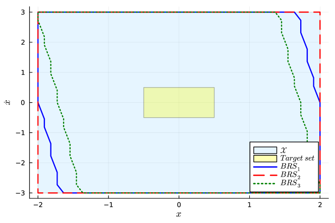
Figure 1: Inner approximations of the presets of $\mathsf{LifSys}_{\mathcal{X}}$ computed using $\mathsf{LifSys}_{i}$ for $i\in\{1,2,3\}$ (denoted $BRS_{i}$).

5 Conclusion and Future Directions

This work introduces a new notion of simulation between lifted control systems. The proposed simulation relation is defined for general set-valued nonlinear and non-autonomous dynamics and is shown to imply containment of both open-loop and closed-loop behaviors. Then, optimization-based sufficient conditions are derived to verify if one lifted system simulates another. These contributions provide a theoretic and algorithmic framework for analyzing lifted systems, and finite-dimensional Koopman approximations in particular. In the future, we will extend our approach to continuous-time and hybrid systems, non-polynomial but Lipschitz systems, and develop algorithms to compute “good” lifting functions.

Acknowledgments: The authors thank Zexiang Liu for insightful discussions on earlier versions of this work.

Appendix A AH-Polytope containment

In this appendix, we derive algebraic sufficient conditions for the inclusion of a sum of AH-polytopes into another. This result is used in Appendix B to derive sufficient algebraic conditions for (11).

The following result from (Sadraddini and Tedrake, 2019, Prop. 2) gives a sufficient condition for the inclusion of an AH polytope in a sum of AH-polytopes. For a positive integer $N$, the notation $[N]\coloneqq\{1,\dots,N\}$ is used.

Lemma 9

Let $\mathcal{X},\mathcal{Y}_{1},\dots,Y_{N}$ be $N+1$ H-polytopes with $\mathcal{X}$ full dimensional. The inclusion $\bar{x}+X\mathcal{X}\subseteq\oplus_{i=1}^{N}\big{(}\bar{y}_{i}+Y_{i}\mathcal{Y}_{i}\big{)}$ holds if there exists $\Lambda_{i}\geq 0$, $\beta_{i}$, $\Gamma_{i}$, for all $i\in[N]$ such that

$$\Lambda_{i}H_{\mathcal{X}}=H_{\mathcal{Y}_{i}}\Gamma_{i},\ \text{and} \ \Lambda_{i}h_{\mathcal{X}}\leq h_{\mathcal{Y}_{i}}+H_{\mathcal{Y}_{i}}\beta_{i}\ \text{for all}\ i\in[N]$$

$$\sum_{i=1}^{N}\bar{y}_{i}-Y_{i}\beta_{i}=\bar{x}\ \text{and}\ \sum_{i=1}^{N}Y_{i}\Gamma_{i}=X.$$

We build on Lemma 9 to obtain a sufficient condition for the inclusion of a sum of AH-polytopes into another.

Lemma 10

Let $\mathcal{X}_{1},\dots,\mathcal{X}_{M},\mathcal{Y}_{1},\dots,\mathcal{Y}_{N}$ be $M+N$ H-polytopes with all the $\mathcal{X}_{i}$ being full dimensional. The inclusion $\bar{x}+\oplus_{i=1}^{M}X_{i}\mathcal{X}_{i}\subseteq\bar{y}+\oplus_{j=1}^{N}Y_{j}\mathcal{Y}_{j}$ holds if there exists $\Lambda_{j,i}\geq 0$, $\Gamma_{j,i}$ and $\beta_{j}$ for all $i\in[M]$ and $j\in[N]$ such that

$$\Lambda_{j,i}H_{\mathcal{X}_{i}}=H_{\mathcal{Y}_{j}} \Gamma_{j,i},\ \text{for all}\ i\in[M]\ \text{and}\ j\in[N]$$ (10a)

$$\sum_{i=1}^{M}\Lambda_{j,i}h_{\mathcal{X}_{i}} \leq h_{\mathcal{Y}_{j}}+H_{\mathcal{Y}_{j}}\beta_{j},\ \text{for all}\ j\in[N]$$ (10b)

$$\bar{y}-\sum_{j=1}^{N}Y_{j}\beta_{j} =\bar{x}$$ (10c)

$$\sum_{j=1}^{N}Y_{j}\Gamma_{j,i} =X_{i},\ \text{for all}\ i\in[M].$$ (10d)

Let us write the Minkowski sum on the left hand side of the inclusion as an AH-polytope: $\oplus_{i=1}^{M}X_{i}\mathcal{X}_{i}=X_{\oplus}\mathcal{X}_{\oplus}$ with $X_{\oplus}=\begin{bmatrix}X_{1}&\dots&X_{M}\end{bmatrix}$, $H_{\oplus}=\text{blk}(H_{\mathcal{X}_{1}},\dots,H_{\mathcal{X}_{M}})$ (where blk denotes a block-diagonal concatenation), and $h_{\oplus}=\begin{bmatrix}h_{\mathcal{X}_{1}}^{\top}&\dots&h_{\mathcal{X}_{M}}^{\top}\end{bmatrix}^{\top}$. The sufficient condition given by Lemma 9 for $\bar{x}+X_{\oplus}\mathcal{X}_{\oplus}\subseteq\bar{y}+\oplus_{j=1}^{N}Y_{j}\mathcal{Y}_{j}$ is that there exists $\Lambda_{j}\geq 0$, $\Gamma_{j}$, and $\beta_{j}$ such that

$$\Lambda_{j}H_{\oplus}=H_{\mathcal{Y},j}\Gamma_{j},\ \text{and}\ \Lambda_{j}h_{\oplus}\leq h_{\mathcal{Y},j}+H_{\mathcal{Y},j}\beta_{j},\ \forall\ j\in[N]$$

$$\bar{y}-\sum_{j=1}^{N}Y_{j}\beta_{j}=\bar{x}\ \text{and}\ \sum_{i=j}^{N}Y_{j}\Gamma_{j}=X_{\oplus}.$$

Writing $\Lambda_{j}=\begin{bmatrix}\Lambda_{j,1}&\dots&\Lambda_{j,M}\end{bmatrix}$ and $\Gamma_{j}=\begin{bmatrix}\Gamma_{j,1}&\dots&\Gamma_{j,M}\end{bmatrix}$ concludes the proof.∎

Appendix B Sufficient condition for (8c)

In this appendix, we derive an algebraic and finite-dimensional sufficient condition for (8c).

For the sake of simplicity, assume $W_{\mathcal{Y}}=W_{\mathcal{Y}}^{x}\times W_{\mathcal{Y}}^{\bar{x}}$ with $W_{\mathcal{Y}}^{x}\subseteq\mathbb{R}^{n_{\mathcal{X}}}$. Then, condition (8c) can be rewritten as (11a) and (11b):

$$(A_{\mathcal{Y}}R-RA_{\mathcal{Z}})^{xx}\mathcal{X}\oplus (B_{\mathcal{Y}}-RB_{\mathcal{Z}})^{x:}\mathcal{U}\oplus A_{\mathcal{Y}}^{x\bar{x}}W^{\bar{x}}_{\rho}$$

$$\oplus W_{\mathcal{Y}}^{x}\subseteq R^{x:}W_{\mathcal{Z}}$$ (11a)

$$(A_{\mathcal{Y}}R-RA_{\mathcal{Z}})^{\bar{x}x}\mathcal{X}\oplus (B_{\mathcal{Y}}-RB_{\mathcal{Z}})^{\bar{x}:}\mathcal{U}\oplus A_{\mathcal{Y}}^{\bar{x}\bar{x}}W^{\bar{x}}_{\rho}$$

$$\oplus W_{\mathcal{Y}}^{\bar{x}}\subseteq R^{\bar{x}:}W_{\mathcal{Z}}\oplus W_{\rho}^{\bar{x}}.$$ (11b)

Using Lemma 10, a sufficient condition for (11a) is (with underlined bilinearities): there exists $\Lambda_{i}\geq 0$, $\Gamma_{i}$, $\beta$, for $i=1,2,3,4$ such that

$$\begin{array}[]{ll}\Lambda_{1}H_{\mathcal{X}}=H_{W_{\mathcal{Z}}}\Gamma_{1}&\Lambda_{2}H_{\mathcal{U}}=H_{W_{\mathcal{Z}}}\Gamma_{2}\\ \Lambda_{3}H_{W_{\rho}^{\bar{x}}}=H_{W_{\mathcal{Z}}}\Gamma_{3}&\Lambda_{4}H_{W_{\mathcal{Y}}^{\bar{x}}}=H_{W_{\mathcal{Z}}}\Gamma_{4}\end{array}$$ (12c)

$$\Lambda_{1}h_{\mathcal{X}}+\Lambda_{2}h_{\mathcal{U}}+{\underline{\Lambda_{3}h_{W_{\rho}^{\bar{x}}}}}+\Lambda_{4}h_{W_{\mathcal{Y}}^{\bar{x}}} \leq h_{W_{\mathcal{Z}}}+H_{W_{\mathcal{Z}}}\beta$$ (12d)

$$R^{x:}\beta=0$$ (12e)

$$\begin{array}[]{ll}R^{x:}\Gamma_{1}=(A_{\mathcal{Y}}R-RA_{\mathcal{Z}})^{xx}&R^{x:}\Gamma_{2}=(B_{\mathcal{Y}}-RB_{\mathcal{Z}})^{x:}\\ R^{x:}\Gamma_{3}=A_{\mathcal{Y}}^{x\bar{x}}&R^{x:}\Gamma_{4}=I\end{array}$$ (12h)

Similarly, a sufficient condition for (11b) is: there exists $$\Lambda_{j,i}\geq 0 \Gamma_{j,i} \beta_{j} i=1,2,3,4 j=1,2$$, , , for and such that

$$\begin{array}[]{ll}\Lambda_{1,1}H_{\mathcal{X}}=H_{W_{\mathcal{Z}}}\Gamma_{1,1}&\Lambda_{1,2}H_{\mathcal{U}}=H_{W_{\mathcal{Z}}}\Gamma_{1,2}\\ \Lambda_{1,3}H_{W_{\rho}^{\bar{x}}}=H_{W_{\mathcal{Z}}}\Gamma_{1,3}&\Lambda_{1,4}H_{W_{\mathcal{Y}}^{\bar{x}}}=H_{W_{\mathcal{Z}}}\Gamma_{1,4}\\ \Lambda_{2,1}H_{\mathcal{X}}=H_{W_{\rho}^{\bar{x}}}\Gamma_{2,1}&\Lambda_{2,2}H_{\mathcal{U}}=H_{W_{\rho}^{\bar{x}}}\Gamma_{2,2}\\ \Lambda_{2,3}H_{W_{\rho}^{\bar{x}}}=H_{W_{\rho}^{\bar{x}}}\Gamma_{2,3}&\Lambda_{2,4}H_{W_{\mathcal{Y}}^{\bar{x}}}=H_{W_{\rho}^{\bar{x}}}\Gamma_{2,4}.\end{array}$$ (12m)

$$\Lambda_{1,1}h_{\mathcal{X}}+\Lambda_{1,2}h_{\mathcal{U}}+{\underline{\Lambda_{1,3}h_{W_{\rho}^{\bar{x}}}}}+\Lambda_{1,4}h_{W_{\mathcal{Y}}^{\bar{x}}} \leq h_{W_{\mathcal{Z}}}+H_{W_{\mathcal{Z}}}\beta_{1}$$ (12n)

$$\Lambda_{2,1}h_{\mathcal{X}}+\Lambda_{2,2}h_{\mathcal{U}}+{\underline{\Lambda_{2,3}h_{W_{\rho}^{\bar{x}}}}}+\Lambda_{2,4}h_{W_{\mathcal{Y}}^{\bar{x}}} \leq h_{W_{\rho}^{\bar{x}}}+H_{W_{\rho}^{\bar{x}}}\beta_{2}$$ (12o)

$${\underline{R^{\bar{x}:}\beta_{1}}}+\beta_{2}=0$$ (12p)

$$\begin{array}[]{ll}{\underline{R^{\bar{x}:}\Gamma_{1,1}}}+\Gamma_{2,1}=(A_{\mathcal{Y}}R-RA_{\mathcal{Z}})^{\bar{x}x}&{\underline{R^{\bar{x}:}\Gamma_{1,3}}}+\Gamma_{2,3}=A_{\mathcal{Y}}^{\bar{x}\bar{x}}\\[2.84544pt] {\underline{R^{\bar{x}:}\Gamma_{1,2}}}+\Gamma_{2,2}=(B_{\mathcal{Y}}-RB_{\mathcal{Z}})^{\bar{x}:}&{\underline{R^{\bar{x}:}\Gamma_{1,4}}}+\Gamma_{2,4}=I.\end{array}$$ (12s)

Overall, condition (8c) holds if (12) holds.

References

- Ahmadi and Majumdar (2019) Ahmadi, A.A. and Majumdar, A. (2019). Dsos and sdsos optimization: more tractable alternatives to sum of squares and semidefinite optimization. SIAM Journal on Applied Algebra and Geometry, 3(2), 193–230.
- Balim et al. (2023) Balim, H., Aspeel, A., Liu, Z., and Ozay, N. (2023). Koopman-inspired implicit backward reachable sets for unknown nonlinear systems. IEEE Control Systems Letters, 7, 2245–2250.
- Colbrook (2023) Colbrook, M.J. (2023). The multiverse of dynamic mode decomposition algorithms. arXiv preprint arXiv:2312.00137.
- Girard and Martin (2011) Girard, A. and Martin, S. (2011). Synthesis for constrained nonlinear systems using hybridization and robust controllers on simplices. IEEE Trans. on Automatic Control, 57(4), 1046–1051.
- Girard and Pappas (2007) Girard, A. and Pappas, G.J. (2007). Approximation metrics for discrete and continuous systems. IEEE Trans. on Automatic Control, 52(5), 782–798.
- Haseli and Cortés (2023) Haseli, M. and Cortés, J. (2023). Generalizing dynamic mode decomposition: Balancing accuracy and expressiveness in koopman approximations. Automatica, 153, 111001.
- Koopman (1931) Koopman, B.O. (1931). Hamiltonian systems and transformation in hilbert space. Proc. of the National Academy of Sciences, 17(5), 315–318.
- Korda and Mezić (2018) Korda, M. and Mezić, I. (2018). Linear predictors for nonlinear dynamical systems: Koopman operator meets model predictive control. Automatica, 93, 149–160.
- Liu and Ozay (2016) Liu, J. and Ozay, N. (2016). Finite abstractions with robustness margins for temporal logic-based control synthesis. Nonlinear Analysis: Hybrid Systems, 22, 1–15.
- Liu et al. (2023) Liu, Z., Ozay, N., and Sontag, E.D. (2023). On the non-existence of immersions for systems with multiple omega-limit sets. IFAC-PapersOnLine, 56(2), 60–64.
- Majumdar et al. (2020) Majumdar, R., Ozay, N., and Schmuck, A.K. (2020). On abstraction-based controller design with output feedback. In Proc. of Intl. Conf. on Hybrid Systems: Computation and Control, 1–11.
- Papachristodoulou and Prajna (2005) Papachristodoulou, A. and Prajna, S. (2005). A tutorial on sum of squares techniques for systems analysis. In Proc. American Control Conf., 2686–2700. IEEE.
- Proctor et al. (2018) Proctor, J.L., Brunton, S.L., and Kutz, J.N. (2018). Generalizing koopman theory to allow for inputs and control. SIAM Journal on Applied Dynamical Systems, 17(1), 909–930.
- Reissig et al. (2016) Reissig, G., Weber, A., and Rungger, M. (2016). Feedback refinement relations for the synthesis of symbolic controllers. IEEE Trans. on Automatic Control, 62(4), 1781–1796.
- Sadraddini and Tedrake (2019) Sadraddini, S. and Tedrake, R. (2019). Linear encodings for polytope containment problems. arXiv preprint arXiv:1903.05214.
- Sankaranarayanan (2016) Sankaranarayanan, S. (2016). Change-of-bases abstractions for non-linear hybrid systems. Nonlinear Analysis: Hybrid Systems, 19, 107–133.
- Tabuada (2009) Tabuada, P. (2009). Verification and control of hybrid systems: a symbolic approach. Springer Science & Business Media.
- Wang et al. (2023) Wang, Z., Jungers, R.M., and Ong, C.J. (2023). Computation of invariant sets via immersion for discrete-time nonlinear systems. Automatica, 147, 110686.
- Williams et al. (2015) Williams, M.O., Kevrekidis, I.G., and Rowley, C.W. (2015). A data–driven approximation of the koopman operator: Extending dynamic mode decomposition. Journal of Nonlinear Science, 25, 1307–1346.
- Zamani et al. (2011) Zamani, M., Pola, G., Mazo, M., and Tabuada, P. (2011). Symbolic models for nonlinear control systems without stability assumptions. IEEE Trans. on Automatic Control, 57(7), 1804–1809.