Benchmark calculations of fully heavy compact and molecular tetraquark states

Abstract

We calculate the mass spectrum of the S-wave fully heavy tetraquark systems $QQ\bar{Q}\bar{Q}~{}(Q=c,b)$ with both “normal” $(J^{PC}=0^{++},1^{+-},2^{++})$ and “exotic” $(J^{PC}=0^{+-},1^{++},2^{+-})$ C-parities using three different quark potential models (AL1, AP1, BGS). The “exotic” C-parity systems refer to the ones that cannot be composed of two S-wave ground heavy quarkonia. We incorporate the molecular dimeson and compact diquark-antidiquark spatial correlations simultaneously, thereby discerning the actual configurations of the states. We employ the Gaussian expansion method to solve the four-body Schrödinger equation, and the complex scaling method to identify the resonant states. The mass spectra in three different models qualitatively agree with each other. We obtain several resonant states with $J^{PC}=0^{++},1^{+-},2^{++},1^{++}$ in the mass region $(6.92,7.30)\,\mathrm{GeV}$, some of which are good candidates of the experimentally observed $X(6900)$ and $X(7200)$. We also obtain several “exotic” C-parity zero-width states with $J^{PC}=0^{+-}$ and $2^{+-}$. These zero-width states have no corresponding S-wave di-quarkonium threshold and can only decay strongly to final states with P-wave quarkonia. With the notation $T_{4Q,J(C)}(M)$, we deduce from the root mean square radii that the $X(7200)$ candidates $T_{4c,0(+)}(7173),T_{4c,2(+)}(7214)$ and the state $T_{4c,1(-)}(7191)$ look like molecular states although most of the resonant and zero-width states are compact states.

I Introduction

Since the discovery of $X(3872)$ [1], numerous candidates for multiquark states have been observed in experiments. The multiquark states exhibit more intricate color structures in forming color-singlet states than the conventional hadrons. Investigating these states can enhance our understanding of Quantum Chromodynamics (QCD). One can find more details in recent reviews [2, 3, 4, 5, 6, 7, 8, 9, 10, 11, 12].

Among the myriad multiquark systems, the fully heavy tetraquark states $QQ\bar{Q}\bar{Q}~{}(Q=b,c)$ stand out as relatively pure and clear systems, unaffected by unquenched dynamics such as the creation and annihilation of light $q\bar{q}~{}(q=u,d,s)$ pairs. Recently, significant progress has been made in the search for fully heavy tetraquark states. The LHCb Collaboration initially discovered a fully charmed tetraquark candidate $X(6900)$ [13]. Subsequently, both the CMS [14] and ATLAS [15] collaborations independently verified the existence of the $X(6900)$ state and reported additional fully charmed tetraquark resonant states. Specifically, the CMS reported the observation of $X(6600)$ and $X(7200)$ [14], while the ATLAS reported the observation of $X(6400)$, $X(6600)$, and $X(7200)$ [15]. Theoretical studies on fully heavy tetraquark states began long before the experiments, making predictions of their existence [16, 17, 18, 19, 20, 21, 22, 23, 24, 25, 26]. After recent discoveries, many theoretical efforts have been made to understand the experimental results [27, 28, 29, 30, 31, 32, 33, 34, 35, 36, 37, 38, 39, 40, 41, 42, 43, 44, 45, 46, 47, 48, 49, 50, 51, 52, 53, 54, 55, 56, 57, 58, 59, 60, 61, 62, 63, 64, 65, 66, 67, 68, 69, 70, 71, 72, 73, 74, 75, 76]. The interpretations of these states include compact tetraquark states [27, 28, 29, 30, 34, 39, 46, 47, 48, 50, 51, 54, 55, 56, 58, 59, 61, 67, 70, 71, 75], dynamical effects in di-charmonium rescattering [35, 36, 42, 43, 52, 60, 63, 64, 65, 72], hybrid states [44], etc. Further details can be found in recent reviews [11, 12].

The nature of fully charmed tetraquark states remains controversial. Currently, few theoretical works consider compact diquark-antidiquark and molecular di-quarkonium spatial configurations simultaneously and perform comprehensive four-body dynamical calculations. In our previous studies [77, 78, 79], we incorporated both dimeson and diquark-antidiquark spatial configurations, employing various quark models and few-body methods to conduct benchmark calculations for tetraquark bound states. We have illustrated that the Gaussian Expansion Method (GEM) is highly efficient in exploring tetraquark states. Our results indicate that there are no bound states in the fully heavy tetraquark systems. In Refs. [68, 73], the authors utilized the GEM to conduct four-body dynamic calculations for the fully charmed tetraquark systems. Furthermore, they employed the complex scaling method (CSM) [80, 81, 82] to distinguish resonant states from di-charmonium scattering states, yielding convincing and intriguing results. However, it is noteworthy that the discussion in Refs. [68, 73] is limited to fully charmed tetraquark states, and does not include an exploration of fully bottomed tetraquark states. Furthermore, the discussion excludes the systems with “exotic” C-parity $(J^{PC}=0^{+-},1^{++},2^{+-})$, which refer to the ones that cannot be composed of two S-wave ground heavy quarkonia.

In this study, we aim to investigate the S-wave fully heavy tetraquark $QQ\bar{Q}\bar{Q}~{}(Q=b,c)$ resonances with all possible quantum numbers, employing a framework that has been used to investigate $Qs\bar{q}\bar{q}$ states efficiently [83]. We employ the GEM to solve the four-body Schrödinger equation, considering both compact diquark-antidiquark and molecular di-quarkonium spatial configurations. We utilize the CSM to distinguish resonant states from di-quarkonium scattering states. Regarding the (anti)quark-(anti)quark interactions, we compare three quark potential models with well-determined parameters and do not introduce any new free parameters. Additionally, we apply the approach proposed in our previous work [83] to analyze the spatial structures of the tetraquark states, which can clearly distinguish the compact tetraquark states and the molecular states.

This paper is organized as follows. In Section II, we provide an introduction to the theoretical framework, including (anti)quark-(anti)quark interactions, calculation methods, and the approach for analyzing the spatial structures of the tetraquark states. In Section III, we comprehensively discuss our numerical results, exploring the masses, widths, decays, and spatial structures of the fully heavy tetraquark states. We also explore the properties of the states with “exotic” C-parity. Finally, we summarize our findings in Section IV.

II Theoretical Framework

II.1 Hamiltonian

In the center-of-mass frame, the nonrelativistic Hamiltonian for a tetraquark system reads

$$H=\sum_{i=1}^{4}(m_{i}+\frac{p_{i}^{2}}{2m_{i}})+\sum_{i<j=1}^{4}V_{ij},$$ (1)

where $m_{i}$ and $p_{i}$ are the mass and momentum of the (anti)quark $i$, respectively. $V_{ij}$ represents the two-body interaction between the (anti)quark pair $(ij)$. In this study, we adopt three different quark potential models, namely the AL1 and AP1 potentials proposed in Refs. [84, 85] and the potential used to study charmonia in Ref. [86] (denoted as the BGS potential hereafter). These three potentials contain the one-gluon-exchange interaction and quark confinement interaction, and can be written as

$$V_{ij}=-\frac{3}{16}\boldsymbol{\lambda}_{i}\cdot\boldsymbol{\lambda}_{j}\left(-\frac{\kappa}{r_{ij}}+\lambda r_{ij}^{p}-\Lambda\right.$$ (2)

$$\left.+\frac{8\pi\kappa^{\prime}}{3m_{i}m_{j}}\frac{\exp\left(-r_{ij}^{2}/r_{0}^{2}\right)}{\pi^{3/2}r_{0}^{3}}\boldsymbol{S}_{i}\cdot\boldsymbol{S}_{j}\right),$$

where $r_{ij}$ is the distance between (anti)quark $i$ and $j$, $\boldsymbol{\lambda}_{i}$ and $\boldsymbol{S}_{i}$ are the $\mathrm{SU}(3)$ color Gell-Mann matrix and the spin operator acting on (anti)quark $i$. The first term in the potential is referred to as the color electric term, and the last term is known as the color magnetic term. In the conventional meson and baryon systems, the color factor $\boldsymbol{\lambda}_{i}\cdot\boldsymbol{\lambda}_{j}$ is always negative and induces a confining interaction, thus all eigenstates of the Hamiltonian must be bound states. However, scattering states of two color-singlet clusters and possible resonant states are allowed in the tetraquark systems, since they have richer inner color structures than the conventional hadrons, and the color factor might take a zero or positive value. The parameters of the models are taken from Refs. [85, 86] and listed in Table 1. The parameters for the AL1 and AP1 potential were determined by fitting the meson spectra across all flavor sectors, while those for the BGS potential were determined by the charmonium spectra. The theoretical masses of the charmonia and bottomonia as well as their root-mean-square (rms) radii calculated from the AP1 potential are listed in Table 2. It can be seen that all three potential models can give a satisfactory description of the meson spectra.

Table 1: The parameters in the AL1, AP1 and BGS quark potential models.

Parameters	AL1 [85]	AP1 [85]	BGS [86]
$p$	1	$\frac{2}{3}$	1
$\kappa$	0.5069	0.4242	0.7281
$\lambda{[\mathrm{GeV}^{p+1}]}$	0.1653	0.3898	0.1425
$\Lambda{\rm[GeV]}$	0.8321	1.1313	0
$\kappa^{\prime}$	1.8609	1.8025	0.7281
$m_{c}{\rm[GeV]}$	1.8360	1.8190	1.4794
$m_{b}{\rm[GeV]}$	5.227	5.206	-
$r_{0c}{\rm[GeV^{-1}]}$	1.4478	1.2583	0.9136
$r_{0b}{\rm[GeV^{-1}]}$	1.1497	0.8928	-

Table 2: The masses (in $\mathrm{MeV}$) of $c\bar{c}$ and $b\bar{b}$ quarkonia in three different quark models, compared with the experimental results taken from Ref. [87]. The rms radii (in fm) of the quarkonia in the AP1 potential are listed in the last column.

Mesons	$m_{\rm Exp.}$	$m_{\rm AL1}$	$m_{\rm AP1}$	$m_{\rm BGS}$	$r^{\rm rms}_{\rm AP1}$
$\eta_{c}$	2984	3006	2982	2982	0.35
$\eta_{c}(2S)$	3638	3608	3605	3630	0.78
$\eta_{c}(3S)$	-	4014	3986	4043	1.15
$J/\psi$	3097	3102	3102	3090	0.40
$\psi(2S)$	3686	3641	3645	3672	0.81
$\psi(3S)$	4039	4036	4011	4072	1.17
$\eta_{b}$	9399	9424	9401	-	0.20
$\eta_{b}(2S)$	9999	10003	10000	-	0.48
$\eta_{b}(3S)$	-	10329	10326	-	0.73
$\Upsilon$	9460	9462	9461	-	0.21
$\Upsilon(2S)$	10023	10012	10014	-	0.49
$\Upsilon(3S)$	10355	10335	10335	-	0.74

II.2 Calculation methods

We use the complex scaling method (CSM) to obtain possible bound and resonant states simultaneously, and we apply the Gaussian expansion method (GEM) to solve the complex-scaled four-body Schrödinger equation. We also introduce a method to determine the C-parity of the neutral tetraquark states by decomposing the Hilbert space.

In the CSM [80, 81, 82], the coordinate $\boldsymbol{r}$ and its conjugate momentum $\boldsymbol{p}$ are transformed as

$$U(\theta)\boldsymbol{r}=\boldsymbol{r}e^{i\theta},\quad U(\theta)\boldsymbol{p}=\boldsymbol{p}e^{-i\theta}.$$ (3)

Under such a transformation, the complex-scaled Hamiltonian is written as

$$H(\theta)=\sum_{i=1}^{4}(m_{i}+\frac{p_{i}^{2}e^{-2i\theta}}{2m_{i}})+\sum_{i<j=1}^{4}V_{ij}(r_{ij}e^{i\theta}),$$ (4)

which is no longer hermitian and has complex eigenvalues $E(\theta)$. According to the ABC theorem [80, 81], the energies of the bound states, resonant states and scattering states can be obtained as the eigenvalues of $H(\theta)$ simultanenously. The bound states (zero-width states) lie on the negative real axis in the energy plane and are not changed by the complex scaling. The resonant states with mass $M_{R}$ and width $\Gamma_{R}$ can be detected at $E_{R}=M_{R}-i\Gamma_{R}/2$ when $2\theta>\left|\operatorname{Arg}(E_{R})\right|$. The scattering states line up along beams starting from threshold energies and rotated clockwise by $2\theta$ from the positive real axis.

To solve the complex-scaled Schrödinger equation, we apply the GEM [88] and expand the wave functions of the S-wave fully heavy tetraquark states with total angular momentum $J$ and C-parity $C$ as

$$\Psi^{J}_{C}(\theta)=\mathcal{A}\sum_{\rm{jac}}\sum_{\alpha,n_{i}}\,C^{(\rm{jac})}_{\alpha,n_{i}}(\theta)\left[\chi_{\alpha}^{J}\Phi^{(\rm{jac})}_{n_{1},n_{2},n_{3}}\right]_{C}.$$ (5)

where $\mathcal{A}$ is the antisymmetric operator of identical particles. $\chi_{\alpha}^{J}$ is the color-spin wave function, given by

$$\chi^{J}_{\bar{3}_{c}\otimes 3_{c},s_{1},s_{2}}=\left[\left(Q_{1}Q_{2}\right)_{\bar{3}_{c}}^{s_{1}}\left(\bar{Q}_{3}\bar{Q}_{4}\right)_{3_{c}}^{s_{2}}\right]_{1_{c}}^{J},$$ (6)

$$\chi^{J}_{6_{c}\otimes\bar{6}_{c},s_{1},s_{2}}=\left[\left(Q_{1}Q_{2}\right)_{6_{c}}^{s_{1}}\left(\bar{Q}_{3}\bar{Q}_{4}\right)_{\bar{6}_{c}}^{s_{2}}\right]_{1_{c}}^{J},$$

for all possible combinations of $s_{1},s_{2},J$. It should be emphasized that one has the flexibility to use either the diquark-antidiquark type color-spin basis in Eq. (6) or the dimeson type color-spin basis, which can be written as

$$\chi^{J}_{1_{c}\otimes 1_{c},s_{1},s_{2}}=\left[\left(Q_{1}\bar{Q}_{3}\right)^{s_{1}}_{1_{c}}\left(Q_{2}\bar{Q}_{4}\right)^{s_{2}}_{1_{c}}\right]_{1_{c}},$$ (7)

$$\chi^{J}_{8_{c}\otimes 8_{c},s_{1},s_{2}}=\left[\left(Q_{1}\bar{Q}_{3}\right)^{s_{1}}_{8_{c}}\left(Q_{2}\bar{Q}_{4}\right)^{s_{2}}_{8_{c}}\right]_{1_{c}}.$$

These two sets of bases are both complete and the transformation between them are shown in Appendix A. It has been demonstrated that the use of different discrete basis functions yields negligible differences once they are complete [79]. The S-wave spatial wave function $\Phi^{(\rm{jac})}_{n_{1},n_{2},n_{3}}$ is written as

$$\Phi^{(\rm{jac})}_{n_{1},n_{2},n_{3}}=\phi_{n_{1}}(r_{jac})\phi_{n_{2}}(\lambda_{jac})\phi_{n_{3}}(\rho_{jac})$$ (8)

where $(\rm{jac})=(a),\,(b),\,(c)$ denotes three sets of spatial configurations (dimeson and diquark-antidiquark) considered in our calculations, and $r_{jac},\lambda_{jac}$, $\rho_{jac}$ are three independent Jacobian coordinates in configuration $(\rm{jac})$, as shown in Fig. 1. $\phi_{n_{i}}(r)$ takes the Gaussian form,

$$\begin{array}[]{c}\phi_{n_{i}}(r)=N_{n_{i}}e^{-\nu_{n_{i}}r^{2}},\\ \nu_{n_{i}}=\nu_{1}\gamma^{n_{i}-1},\end{array}$$ (9)

where $N_{n_{i}}$ is the normalization factor. Finally, the expansion coefficients $C^{(\rm{jac})}_{\alpha,n_{i}}(\theta)$ are determined by solving the energy eigenvalue equation,

$$H(\theta)\Psi_{C}^{J}(\theta)=E(\theta)\Psi_{C}^{J}(\theta).$$ (10)

For the fully heavy neutral tetraquark system $(QQ\bar{Q}\bar{Q})$, the eigenstates of the Hamiltonian have definite C-parity $C$. To determine the C-parity of the obtained states, we decompose the Hilbert space $\mathcal{H}$ into $\mathcal{H}_{+}$ and $\mathcal{H}_{-}$, where $\mathcal{H}_{\pm}$ represents the subspace with $C=\pm 1$. Under charge conjugation, the basis functions with $(\rm{jac})=(a)$ are transformed as

$$[(Q_{1}Q_{2})^{s_{1}}_{x_{c}}(\bar{Q}_{3}\bar{Q}_{4})^{s_{2}}_{\bar{x}_{c}}]^{J}_{1_{c}}\Phi^{(\rm{a})}_{n_{1},n_{2},n_{3}}$$ (11)

$$\stackrel{{\scriptstyle\mathbf{C}}}{{\rightarrow}} [(\bar{Q}_{1}\bar{Q}_{2})^{s_{1}}_{\bar{x}_{c}}({Q}_{3}{Q}_{4})^{s_{2}}_{x_{c}}]^{J}_{1_{c}}\Phi^{(\rm{a})}_{n_{1},n_{2},n_{3}}$$

$$= (-1)^{s_{1}+s_{2}-J}[({Q}_{3}{Q}_{4})^{s_{2}}_{{x_{c}}}(\bar{Q}_{1}\bar{Q}_{2})^{s_{1}}_{\bar{x}_{c}}]^{J}_{1_{c}}\Phi^{(\rm{a})}_{n_{1},n_{2},n_{3}}$$

$$= (-1)^{s_{1}+s_{2}-J}[(Q_{1}Q_{2})^{s_{2}}_{{x_{c}}}(\bar{Q}_{3}\bar{Q}_{4})^{s_{1}}_{\bar{x}_{c}}]^{J}_{1_{c}}\Phi^{(\rm{a})}_{n_{1},n_{2},n_{3}}.$$

In the third line, we exchange $[{Q}_{3}{Q}_{4}]^{s_{2}}_{x_{c}}$ and $[\bar{Q}_{1}\bar{Q}_{2}]^{s_{1}}_{\bar{x}_{c}}$ in the color-spin wave function and the factor $(-1)^{s_{1}+s_{2}-J}$ arises from the Clebsch–Gordan coefficient. In the last line the particle indices $1\leftrightarrow 3,2\leftrightarrow 4$ are exchanged to rewrite the basis function to its original form. The transformation behaviour of the basis functions with $(\rm{jac})=(b),(c)$ can be obtained similarly,

$$[(Q_{1}Q_{2})^{s_{1}}_{x_{c}}(\bar{Q}_{3}\bar{Q}_{4})^{s_{2}}_{\bar{x}_{c}}]^{J}_{1_{c}}\Phi^{(\rm{b})}_{n_{1},n_{2},n_{3}}$$ (12)

$$\stackrel{{\scriptstyle\mathbf{C}}}{{\rightarrow}} (-1)^{s_{1}+s_{2}-J}[(Q_{1}Q_{2})^{s_{2}}_{{x_{c}}}(\bar{Q}_{3}\bar{Q}_{4})^{s_{1}}_{\bar{x}_{c}}]^{J}_{1_{c}}\Phi^{(\rm{b})}_{n_{2},n_{1},n_{3}},$$

$$[(Q_{1}Q_{2})^{s_{1}}_{x_{c}}(\bar{Q}_{3}\bar{Q}_{4})^{s_{2}}_{\bar{x}_{c}}]^{J}_{1_{c}}\Phi^{(\rm{c})}_{n_{1},n_{2},n_{3}}$$ (13)

$$\stackrel{{\scriptstyle\mathbf{C}}}{{\rightarrow}} (-1)^{s_{1}+s_{2}-J}[(Q_{1}Q_{2})^{s_{2}}_{x_{c}}(\bar{Q}_{3}\bar{Q}_{4})^{s_{1}}_{\bar{x}_{c}}]^{J}_{1_{c}}\Phi^{(\rm{c})}_{n_{2},n_{1},n_{3}}.$$

For these two sets of spatial configurations, the indices of Gaussian basis $(n_{1},n_{2})$ are swapped. Once we obtain the transformation properties, we can construct the basis of $\mathcal{H}_{\pm}$ by using linear superposition of the original basis functions. The basis functions of $\mathcal{H}_{\pm}$ that satisfy the antisymmetrization of identical fermions are listed in Appendix B. The Hamiltonian is block-diagonal in $\mathcal{H}=\mathcal{H}_{+}\oplus\mathcal{H}_{-}$ because of the conservation of C-parity, and we can obtain states with $C=\pm 1$ by solving the Schrödinger equation in $\mathcal{H}_{\pm}$ separately.

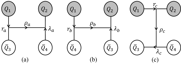
Figure 1: The Jacobian coordinates for two types of spatial configurations: (a), (b) for the dimeson configurations, and (c) for the diquark-antidiquark configuration.

II.3 Spatial structures

Basically, the molecular or compact tetraquark states can be discerned through the analysis of their spatial configurations. The root-mean-square (rms) radius between different quarks is a commonly used criterion. However, the naive definition of the rms radius could be misleading when the antisymmetric wave function is required for the identical quarks. For instance, when the mesons $(c\bar{q})$ and $(s\bar{q})$ form a molecular state, the wave function satisfying the Pauli principle is $|\psi_{\mathcal{A}}\rangle=|(c\bar{q}_{1})(s\bar{q}_{2})\rangle-|(c\bar{q}_{2})(s\bar{q}_{1})\rangle$. One can see that each antiquark $\bar{q}$ belongs to both mesons simultaneously. Therefore, neither $\langle\psi_{\mathcal{A}}|r_{c\bar{q}}^{2}|\psi_{\mathcal{A}}\rangle$ nor $\langle\psi_{\mathcal{A}}|r_{s\bar{q}}^{2}|\psi_{\mathcal{A}}\rangle$ can reflect the size of the constituent mesons.

In Ref. [83], we proposed a new approach to calculate the rms radii in the $Qs\bar{q}\bar{q}$ system, which eliminates the ambiguity arising from the antisymmetrization of identical pariticles $\bar{q}\bar{q}$. In the fully heavy tetraquark system, there exist two pairs of identical particles. Here we further extend the definitions of rms radii for the $QQ\bar{Q}\bar{Q}$ system. We uniquely decompose the antisymmetric wave function as

$$\Psi^{J}(\theta)= \sum_{s_{1}\leq s_{2}}\left([(Q_{1}\bar{Q}_{3})^{s_{1}}_{1_{c}}(Q_{2}\bar{Q}_{4})^{s_{2}}_{1_{c}}]^{J}_{1_{c}}\otimes|\psi_{1}^{s_{1}s_{2}}(\theta)\rangle\right.$$ (14)

$$+[(Q_{1}\bar{Q}_{3})^{s_{2}}_{1_{c}}(Q_{2}\bar{Q}_{4})^{s_{1}}_{1_{c}}]^{J}_{1_{c}}\otimes|\psi_{2}^{s_{1}s_{2}}(\theta)\rangle$$

$$+[(Q_{1}\bar{Q}_{4})^{s_{1}}_{1_{c}}(Q_{2}\bar{Q}_{3})^{s_{2}}_{1_{c}}]^{J}_{1_{c}}\otimes|\psi_{3}^{s_{1}s_{2}}(\theta)\rangle$$

$$+\left.[(Q_{1}\bar{Q}_{4})^{s_{2}}_{1_{c}}(Q_{2}\bar{Q}_{3})^{s_{1}}_{1_{c}}]^{J}_{1_{c}}\otimes|\psi_{4}^{s_{1}s_{2}}(\theta)\rangle\right)$$

$$= \mathcal{A}\sum_{s_{1}\leq s_{2}}[(Q_{1}\bar{Q}_{3})^{s_{1}}_{1_{c}}(Q_{2}\bar{Q}_{4})^{s_{2}}_{1_{c}}]^{J}_{1_{c}}\otimes|\psi_{1}^{s_{1}s_{2}}(\theta)\rangle,$$

where $s_{1},s_{2}$ sum over spin configurations with total angular momentum $J$. We denote the non-antisymmetric component of the wave function as

$$|\Psi_{\mathrm{nA}}^{J}(\theta)\rangle=\sum_{s_{1}\leq s_{2}}[(Q_{1}\bar{Q}_{3})^{s_{1}}_{1_{c}}(Q_{2}\bar{Q}_{4})^{s_{2}}_{1_{c}}]^{J}_{1_{c}}\otimes|\psi_{1}^{s_{1}s_{2}}(\theta)\rangle.$$ (15)

where $(Q_{1}\bar{Q}_{3})$ and $(Q_{2}\bar{Q}_{4})$ form color singlets. Instead of using the whole wave function $\Psi^{J}(\theta)$, we use $|\Psi_{\mathrm{nA}}^{J}(\theta)\rangle$ to define the rms radius:

$$r^{\mathrm{rms}}_{ij}\equiv\mathrm{Re}\left[\sqrt{\frac{\langle\Psi_{\mathrm{nA}}^{J}(\theta)|r_{ij}^{2}e^{2i\theta}|\Psi_{\mathrm{nA}}^{J}(\theta)\rangle}{\langle\Psi_{\mathrm{nA}}^{J}(\theta)|\Psi_{\mathrm{nA}}^{J}(\theta)\rangle}}\right].$$ (16)

It should be emphasized that the inner products in the CSM are defined using the c-product [89],

$$\langle\phi_{n}\mid\phi_{m}\rangle\equiv\int\phi_{n}(r)\phi_{m}(r)d^{3}r,$$ (17)

where the square of the wave function rather than the square of its magnitude is used. The rms radius calculated by the c-product is generally not real, but its real part can still reflect the internal quark clustering behavior if the resonant state is not too broad, as discussed in Ref. [90].

We can investigate the internal spatial structures of the tetraquark states by analyzing the rms radii. For example, if the resulting state is a scattering state or a hadronic molecule of $\eta_{c}J/\psi$, $r_{c_{1}\bar{c}_{3}}$ and $r_{c_{2}\bar{c}_{4}}$ are respectively expected to be the sizes of $\eta_{c}$ and $J/\psi$, and much smaller than the other rms radii. On the other hand, if the resulting state is a compact tetraquark state, all rms radii in the four-body system should be of the same order. However, it should be noted that for a hadronic molecule composed of two mesons with the same quantum numbers but different radial excitation, for example $\psi(3S)J/\psi$, the current definition cannot eliminate the ambiguity arising from the antisymmetrization. As a result, neither $r_{c_{1}\bar{c}_{3}}$ nor $r_{c_{2}\bar{c}_{4}}$ reflects the size of $\psi(3S)$ or $J/\psi$; instead, they represent the average of the sizes of the two mesons.

III Results and Discussions

We investigate the S-wave fully charmed $cc\bar{c}\bar{c}$ and fully bottomed $bb\bar{b}\bar{b}$ tetraquark systems with all possible quantum numbers, including $J^{PC}=0^{++},1^{+-},2^{++},0^{+-},1^{++},2^{+-}$. It should be stressed that the S-wave ground state di-quarkonium thresholds exist only in the $0^{++},1^{+-},2^{++}$ systems, namely $\eta_{c}\eta_{c}$ and $\eta_{b}\eta_{b}$ in the $0^{++}$ systems, $\eta_{c}J/\psi$ and $\eta_{b}\Upsilon$ in the $1^{+-}$ systems, $J/\psi J/\psi$ and $\Upsilon\Upsilon$ in the $2^{++}$ systems. In the following discussions, the $0^{++},1^{+-},2^{++}$ systems are referred to as “normal” C-parity systems, whereas the $0^{+-},1^{++},2^{+-}$ systems are referred to as “exotic” C-parity systems. For convenience, we label the $QQ\bar{Q}\bar{Q}$ tetraquark states obtained in the calculations as $T_{4Q,J(C)}(M)$, where $M$ is the mass of the state.

III.1 Fully charmed tetraquark

III.1.1 States with “normal” C-parity

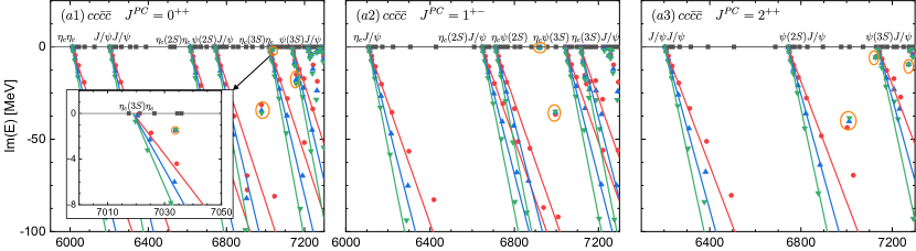
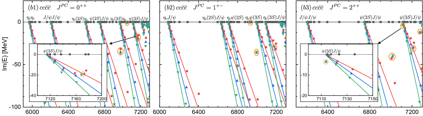
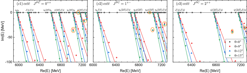
Figure 2: The complex energy eigenvalues of the $cc\bar{c}\bar{c}$ states with “normal” C-parity in the (a) AL1, (b) AP1 and (c) BGS potential with varying $\theta$ in the CSM. The solid lines represent the continuum lines rotating along $\operatorname{Arg}(E)=-2\theta$. The resonances do not shift as $\theta$ changes and are highlighted by the orange circles.

With the CSM, the complex eigenenergies of the $0^{++},1^{+-},2^{++}$ $cc\bar{c}\bar{c}$ systems obtained from three different quark potential models are shown in Fig. 2. We choose varying complex scaling angles $\theta$ to distinguish resonant states from scattering states. All of the states are above the lowest di-quarkonium threshold, so no bound state is obtained. The di-quarkonium scattering states rotate along the continuum lines starting from the threshold energies. Moreover, we obtain a series of resonant states whose complex energies are summarized in Table 3. For comparison, we also list the results in Ref. [68], where the authors used the BGS potential for the $cc\bar{c}\bar{c}$ systems.

Qualitatively, the $cc\bar{c}\bar{c}$ resonances obtained from three different quark potential models are in accordance with each other. Most of the resonances exist in all three models. For a specific resonant state, its width remains consistent across different models, while the mass in the BGS potential is approximately $50$-$100$ $\mathrm{MeV}$ larger than those in the AL1 and AP1 potentials. These differences are expected considering that the discrepancies of the predictions of the heavy quarkonium mass spectra from various potentials are up to tens of $\mathrm{MeV}$.

The tetraquark resonant states with different quantum numbers $J^{PC}$ exhibit a similar pattern. A lower resonant state with mass $M\approx 7000\,\mathrm{MeV}$ and width $\Gamma\approx 75\,\mathrm{MeV}$, and a higher resonant state with mass $M\approx 7200\,\mathrm{MeV}$ and width $\Gamma\approx 50\,\mathrm{MeV}$ are obtained in the $0^{++},1^{+-},2^{++}$ systems. The lower $0^{++}$ state can decay into the $\eta_{c}\eta_{c},J/\psi J/\psi,\eta_{c}(2S)\eta_{c}$ and $\psi(2S)J/\psi$ channels. Additionally, the higher $0^{++}$ state can decay into the $\eta_{c}(3S)\eta_{c}$ and $\psi(3S)J/\psi$ channels. The lower $2^{++}$ state can decay into the $J/\psi J/\psi$ and $\psi(2S)J/\psi$ channels. Additionally, the higher $2^{++}$ state can decay into the $\psi(3S)J/\psi$ channel. Considering that the quark potential models have errors up to tens of $\mathrm{MeV}$ and that we have neglected the widths of the quarkonia in our calculations, the lower $0^{++}$ and $2^{++}$ states may serve as the candidates for the experimentally observed $X(6900)$ state, while the higher $0^{++}$ and $2^{++}$ states may serve as the candidates for the experimentally observed $X(7200)$ state. On the other hand, the lower $1^{+-}$ state can decay into the $\eta_{c}J/\psi,\eta_{c}(2S)J/\psi$ and $\eta_{c}\psi(2S)$ channels. Additionally, the higher $1^{+-}$ state can decay into the $\eta_{c}\psi(3S)$ and $\eta_{c}(3S)J/\psi$ channels. The $1^{+-}$ states are not the candidates for $X(6900)$ or $X(7200)$ because they can not decay into either the $J/\psi J/\psi$ or $\psi(2S)J/\psi$ channels. These states can be searched for in future experiments.

Moreover, we observe several narrow resonant states with different quantum numbers. These states are found in the mass region $(6.92,7.30)\,\mathrm{GeV}$. These narrow resonances can be searched for by experiments in the corresponding di-quarkonium decay channels. However, we do not observe any signal for resonance in the mass region $(6.2,6.6)\,\mathrm{GeV}$, namely no candidate for $X(6400)$ or $X(6600)$ is found.

Comparing the results of resonant states obtained from the BGS potential with those of Ref. [68], our calculations can reproduce the previous results well within numerical uncertainty. In addition, we obtain three extra narrow resonant states in the BGS potential. The reason for these discrepancies might be that a set of complete color-spin basis is used in our calculations while some basis functions are neglected in Ref. [68]. For example, in the $0^{++}$ system, the di-quarkonium color configuration $[(Q_{1}\bar{Q}_{3})_{8_{c}}(Q_{2}\bar{Q}_{4})_{8_{c}}]_{1_{c}}$ is not included in the previous calculations. These missing basis functions turn out to be crucial for the existence of the extra resonant states.

As mentioned above, the fully charmed tetraquark resonant states obtained from different models qualitatively agree with each other. Therefore, we only choose the results in the AP1 potential to analyze their inner structures. The proportions of the color configurations $\chi_{\bar{3}_{c}\otimes 3_{c}}$ and $\chi_{6_{c}\otimes\bar{6}_{c}}$ in the wave functions as well as the rms radii of the fully charmed resonant states are listed in Table 4. For most resonant states, their rms radii are approximately of the same size and less than $1$ fm, indicating that they are compact tetraquark states. However, for the $X(7200)$ candidate states $T_{4c,0(+)}(7173),T_{4c,2(+)}(7214)$ and the state $T_{4c,1(-)}(7191)$ , the $r^{\rm rms}_{c_{1}\bar{c}_{3}}$ and $r^{\rm rms}_{c_{2}\bar{c}_{4}}$ are much smaller than the other radii. Compared with the rms radii of the quarkonia listed in Table 2, we observe that both $r^{\rm rms}_{c_{1}\bar{c}_{3}}$ and $r^{\rm rms}_{c_{2}\bar{c}_{4}}$ are larger than the rms radii of $\eta_{c}$ and $J/\psi$, and smaller than those of $\eta_{c}(3S)$ and $\psi(3S)$, while $r^{\rm rms}_{c_{1}\bar{c}_{4}},r^{\rm rms}_{c_{2}\bar{c}_{3}},r^{\rm rms}_{c_{1}c_{2}}$ and $r^{\rm rms}_{\bar{c}_{3}\bar{c}_{4}}$ are much larger than the rms radii of all mesons. These results suggest that these three states might have a molecular configuration. It should be noted that these resonant states have relatively large widths and are located close to the continuum line of the scattering states, therefore the results of their rms radii are less numerically accurate in the CSM and should be considered as qualitative estimates.

Table 3: The complex energies $E=M-i\Gamma/2$ (in $\mathrm{MeV}$) of the $cc\bar{c}\bar{c}$ resonant states with “normal” C-parity from various potential models. The last column lists the results in Ref. [68]. The “?” indicates the potential existence of resonant states, which blend into the continuum lines of scattering states and cannot be obtained accurately in the present calculations. The “-” suggests that no corresponding resonance is obtained.

$J^{PC}$	AL1	AP1	BGS	BGS, Wang et al.
$0^{++}$	$6980-35i$	$6978-36i$	$7030-36i$	$7035-39i$
	$7034-1i$	$7049-1i$	$7127-0.1i$	-
	$7156-20i$	$7173-20i$	$7239-17i$	$7202-30i$
$1^{+-}$	$6921-0.5i$	$6932-0.5i$	$6991-0.1i$	-
	$6995-35i$	$6998-35i$	$7048-35i$	$7050-35i$
	?	$7191-32i$	$7254-24i$	$7273-25i$
$2^{++}$	$7013-38i$	$7017-39i$	$7066-39i$	$7068-42i$
	$7127-6i$	$7114-4i$	-	-
	?	$7214-30i$	$7268-32i$	$7281-46i$
	$7272-9i$	$7276-12i$	$7337-8i$	-

Table 4: The proportions of different color configurations and the rms radii (in fm) of the $cc\bar{c}\bar{c}$ resonant states with “normal” C-parity in the AP1 potential. The last column shows the spatial configurations of the states, where C. and M. represent the compact tetraquark and molecular configurations, respectively.

$J^{PC}$	$M-i\Gamma/2$	$\chi_{\bar{3}_{c}\otimes 3_{c}}$	$\chi_{6_{c}\otimes\bar{6}_{c}}$	$r_{c_{1}\bar{c}_{3}}^{\mathrm{rms}}$	$r_{c_{2}\bar{c}_{4}}^{\mathrm{rms}}$	$r_{c_{1}\bar{c}_{4}}^{\mathrm{rms}}$=$r_{c_{2}\bar{c}_{3}}^{\mathrm{rms}}$	$r_{c_{1}c_{2}}^{\mathrm{rms}}$=$r_{\bar{c}_{3}\bar{c}_{4}}^{\mathrm{rms}}$	Configurations
$0^{++}$	$6978-36i$	$86\%$	$14\%$	$0.81$	$0.81$	$0.86$	$0.66$	C.
	$7049-1i$	$37\%$	$63\%$	$0.70$	$0.70$	$0.82$	$0.75$	C.
	$7173-20i$	$46\%$	$54\%$	$0.89$	$0.89$	$2.31$	$2.28$	M.
$1^{+-}$	$6932-0.5i$	$65\%$	$35\%$	$0.66$	$0.66$	$0.73$	$0.63$	C.
	$6998-35i$	$88\%$	$12\%$	$0.79$	$0.80$	$0.77$	$0.59$	C.
	$7191-32i$	$44\%$	$56\%$	$0.71$	$1.08$	$2.09$	$2.08$	M.
$2^{++}$	$7017-39i$	$90\%$	$10\%$	$0.79$	$0.79$	$0.71$	$0.56$	C.
	$7114-4i$	$69\%$	$31\%$	$0.92$	$0.92$	$0.65$	$0.55$	C.
	$7214-30i$	$57\%$	$43\%$	$0.92$	$0.92$	$1.93$	$1.88$	M.
	$7276-12i$	$73\%$	$27\%$	$0.86$	$0.86$	$1.04$	$0.93$	C.

III.1.2 States with “exotic” C-parity

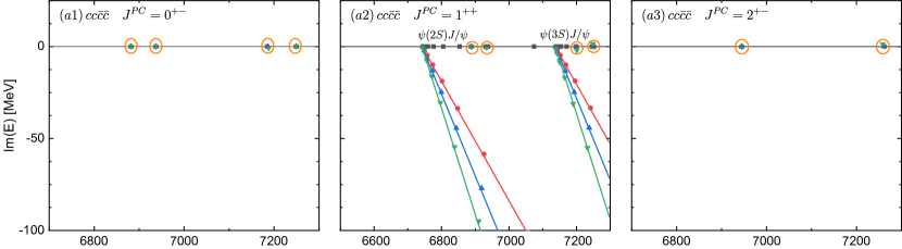
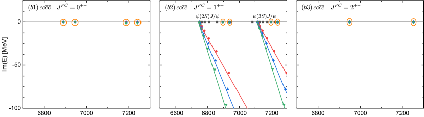
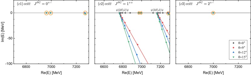
Figure 3: The complex energy eigenvalues of the $cc\bar{c}\bar{c}$ states with “exotic” C-parity in the (a) AL1, (b) AP1 and (c) BGS potential with varying $\theta$ in the CSM. The solid lines represent the continuum lines rotating along $\operatorname{Arg}(E)=-2\theta$. The zero-width states and resonances do not shift as $\theta$ changes and are highlighted by the orange circles.

The complex eigenenergies of the fully charmed tetraquark systems with “exotic” C-parity $(J^{PC}=0^{+-},1^{++},2^{+-})$ obtained from three different quark potential models are shown in Fig. 3. We obtain a series of resonant and zero-width states, whose energies are summarized in Table 5. Similar to the systems with “normal” C-parity, the states with “exotic” C-parity obtained from different models qualitatively agree with each other. The masses of a specific state in the AL1 and AP1 potentials are nearly the same, while the mass in the BGS potential is around $50$-$100$ $\mathrm{MeV}$ larger than the former ones. In the following we solely focus on the results in the AP1 potential. The proportions of the color configurations and the rms radii of the resonant and zero-width states are listed in Table 6. The different rms radii of these states are approximately the same and less than 1 fm, indicating that all of these states have compact tetraquark configuration.

For the $1^{++}$ $cc\bar{c}\bar{c}$ system, we obtain a series of $\psi(2S)J/\psi$ and $\psi(3S)J/\psi$ di-quarkonium scattering states as well as four extremely narrow resonant states, whose two-body decay widths are less than $1$ $\mathrm{MeV}$. The states $T_{4c,1(+)}(6939)$ and $T_{4c,1(+)}(7242)$ have predominant color configuration $\chi_{\bar{3}_{c}\otimes 3_{c}}$. For the states $T_{4c,1(+)}(6896)$ and $T_{4c,1(+)}(7200)$, the proportions of $\chi_{\bar{3}_{c}\otimes 3_{c}}$ and $\chi_{6_{c}\otimes\bar{6}_{c}}$ are around $\frac{2}{3}$ and $\frac{1}{3}$, respectively. Compared with the transformation between different color configurations shown in Appendix A, the predominant color configuration of these two states is actually $\chi_{8_{c}\otimes 8_{c}}$. The states $T_{4c,1(+)}(7200)$ and $T_{4c,1(+)}(7242)$ are the radial excitation of $T_{4c,1(+)}(6896)$ and $T_{4c,1(+)}(6939)$, respectively. All of the four states can decay into the $\psi(2S)J/\psi$ channel, but the decay widths are very small. In Sec. III.3, we discuss the reasons for the small widths in detail.

For the $0^{+-}$ $cc\bar{c}\bar{c}$ system, there do no exist any S-wave di-quarkonium thresholds. Therefore no meson-meson scattering state is observed. All of the states in the system are identified as zero-width states, which lie on the real axis and are not changed by the complex scaling. According to the proportions of color configurations listed in Table 6, the four $0^{+-}$ zero-width states can be clearly arranged into two doublets, $\left\{T_{4c,0(-)}(6890),T_{4c,0(-)}(6945)\right\}$ and $\left\{T_{4c,0(-)}(7188),T_{4c,0(-)}(7242)\right\}$. The color configurations of the two states inside a doublet are orthogonal to each other. The lower state is dominated by the $\chi_{6_{c}\otimes\bar{6}_{c}}$ component, while the higher state is dominated by the $\chi_{\bar{3}_{c}\otimes 3_{c}}$ component. In the fully heavy tetraquark system, it is known that the color magnetic term is suppressed by the heavy quark mass, and the dominant color electric interactions between two (anti)quarks are attractive in $[Q_{1}Q_{2}]_{\bar{3}_{c}}$ and $[\bar{Q}_{3}\bar{Q}_{4}]_{3_{c}}$ configurations but repulsive in $[Q_{1}Q_{2}]_{6_{c}}$ and $[\bar{Q}_{3}\bar{Q}_{4}]_{\bar{6}_{c}}$ configurations. Besides, the color electric term also provides an attractive interaction between the $6_{c}$ diquark and $\bar{6}_{c}$ antidiquark, which is much stronger than the one between $\bar{3}_{c}$ diquark and $3_{c}$ antidiquark due to the color SU(3) algebra [25, 27, 18]. The fact that the lower state has the dominant $\chi_{6_{c}\otimes\bar{6}_{c}}$ configuration suggests that the strong attraction between two color sextet clusters prevails over the repulsion within the (anti)diquark and contributes to the formation of a deeper state than the $\chi_{\bar{3}_{c}\otimes 3_{c}}$ dominant one, which is consistent with the conclusion in Refs. [25, 18]. As a result of the interaction mechanism, the rms radii $r^{\rm rms}_{c_{1}c_{2}}$ and $r^{\rm rms}_{\bar{c}_{3}\bar{c}_{4}}$, which characterize the sizes of the diquark and antidiquark, take larger values in the $\chi_{6_{c}\otimes\bar{6}_{c}}$ dominant state than in the $\chi_{\bar{3}_{c}\otimes 3_{c}}$ dominant state. On the other hand, the rms radii $r^{\rm rms}_{c_{1}\bar{c}_{3}}$, $r^{\rm rms}_{c_{2}\bar{c}_{4}}$, $r^{\rm rms}_{c_{1}\bar{c}_{4}}$ and $r^{\rm rms}_{c_{2}\bar{c}_{3}}$, which characterize the distance between diquark and antidiquark, take smaller values in the $\chi_{6_{c}\otimes\bar{6}_{c}}$ dominant state than in the $\chi_{\bar{3}_{c}\otimes 3_{c}}$ dominant state. The higher doublet states $\left\{T_{4c,0(-)}(7188),T_{4c,0(-)}(7242)\right\}$ have larger rms radii than the lower doublet states $\left\{T_{4c,0(-)}(6890),T_{4c,0(-)}(6945)\right\}$ and can be viewed as the radial excitation of the latter.

Similar to the $0^{+-}$ system, S-wave di-quarkonium threshold does not exist in the $2^{+-}$ $cc\bar{c}\bar{c}$ system, and all of the states in the system are identified as zero-width states. Due to the restriction of antisymmetrization of identical particles, the only allowed color configuration for these states is $\chi_{\bar{3}_{c}\otimes 3_{c}}$. The state $T_{4c,2(-)}(7252)$ is the radial excitation of the ground state $T_{4c,2(-)}(6950)$.

It should be noted that although S-wave di-quarkonium threshold does not exist in the $0^{+-}$ and $2^{+-}$ $cc\bar{c}\bar{c}$ systems, di-quarkonium thresholds with higher orbital angular momentum do exist in these systems. For example, the P-wave $J/\psi\chi_{c1}$ state and the S-wave $h_{c}\chi_{c1}$ state can form the $0^{+-}$ or $2^{+-}$ $cc\bar{c}\bar{c}$ system, while the S-wave $\eta_{c}\psi_{2}$ state and the P-wave $J/\psi\chi_{c2}$ can form the $2^{+-}$ $cc\bar{c}\bar{c}$ system. These scattering states have the same quantum numbers as the zero-width states obtained in the present calculations. The coupling between them may alter the positions of the zero-width states. Considering the effect of this coupling is beyond the scope of this work. However, if one assumes the coupling effect is small and treats it as perturbation, the positions of the states should not change by much. The zero-width states may obtain nonzero widths and transform into resonant states, which can decay into the di-quarkonium channels with lower energies. All of these states lie above the ground state di-quarkonium threshold $J/\psi\chi_{c1}$, whose theoretical energy in the AP1 potential is $6593\,\mathrm{MeV}$. Therefore, they may be searched for in the P-wave $J/\psi\chi_{c1}$ decay channel in the experiment.

Table 5: The complex energies $E=M-i\Gamma/2$ (in $\mathrm{MeV}$) of the $cc\bar{c}\bar{c}$ resonant and zero-width states with “exotic” C-parity from various potential models.

$J^{PC}$	AL1	AP1	BGS
$0^{+-}$	$6882$	$6890$	$6962$
	$6938$	$6945$	$6995$
	$7185$	$7188$	$7268$
	$7249$	$7242$	$7316$
$1^{++}$	$6889-0.1i$	$6896-0.2i$	$6970-0.1i$
	$6933-0.4i$	$6939-0.4i$	$6995-0.1i$
	$7200-0.4i$	$7200-0.1i$	$7286-0.4i$
	$7251-0.1i$	$7242-0.3i$	$7318-0.2i$
$2^{+-}$	$6945$	$6950$	$6999$
	$7262$	$7252$	$7324$

Table 6: The proportions of different color configurations and the rms radii (in fm) of the $cc\bar{c}\bar{c}$ resonant and zero-width states with “exotic” C-parity in the AP1 potential. The last column shows the spatial configurations of the states, where C. and M. represent the compact tetraquark and molecular configurations, respectively.

$J^{PC}$	$M-i\Gamma/2$	$\chi_{\bar{3}_{c}\otimes 3_{c}}$	$\chi_{6_{c}\otimes\bar{6}_{c}}$	$r_{c_{1}\bar{c}_{3}}^{\mathrm{rms}}$	$r_{c_{2}\bar{c}_{4}}^{\mathrm{rms}}$	$r_{c_{1}\bar{c}_{4}}^{\mathrm{rms}}$=$r_{c_{2}\bar{c}_{3}}^{\mathrm{rms}}$	$r_{c_{1}c_{2}}^{\mathrm{rms}}$=$r_{\bar{c}_{3}\bar{c}_{4}}^{\mathrm{rms}}$	Configuration
$0^{+-}$	$6890$	$36\%$	$64$%	$0.62$	$0.62$	$0.62$	$0.71$	C.
	$6945$	$64\%$	$36\%$	$0.65$	$0.65$	$0.65$	$0.71$	C.
	$7188$	$18\%$	$82\%$	$0.80$	$0.80$	$0.80$	$0.93$	C.
	$7242$	$82\%$	$18\%$	$0.85$	$0.85$	$0.85$	$0.83$	C.
$1^{++}$	$6896-0.2i$	$71\%$	$29\%$	$0.67$	$0.58$	$0.71$	$0.63$	C.
	$6939-0.4i$	$96\%$	$4\%$	$0.60$	$0.68$	$0.65$	$0.68$	C.
	$7200-0.1i$	$68\%$	$32\%$	$0.83$	$0.75$	$0.94$	$0.78$	C.
	$7242-0.3i$	$98\%$	$2\%$	$0.82$	$0.88$	$0.85$	$0.81$	C.
$2^{+-}$	$6950$	$100\%$	$0\%$	$0.65$	$0.65$	$0.65$	$0.69$	C.
	$7252$	$100\%$	$0\%$	$0.86$	$0.86$	$0.86$	$0.81$	C.

III.2 Fully bottomed tetraquark

In the $cc\bar{c}\bar{c}$ system, we observe that the results in different quark potential models qualitatively agree with each other. Therefore, we only choose the AP1 potential to investigate the $bb\bar{b}\bar{b}$ system. The complex eigenenergies of the $bb\bar{b}\bar{b}$ states with “normal” and “exotic” C-parities are shown in Fig. 4.

Similar to the $cc\bar{c}\bar{c}$ system, we obtain a series of resonant states with “normal” C-parity in the $bb\bar{b}\bar{b}$ system. The complex energies, the proportions of different color configurations and the rms radii of these resonant states are listed in Table 7. The different rms radii of these states are around $0.5$ fm, indicating that all of these states have compact tetraquark configuration. We obtain a lower resonant state with mass $M\approx 19780\,\mathrm{MeV}$ and width $\Gamma\approx 60\,\mathrm{MeV}$, and a higher resonant state with mass $M\approx 19950\,\mathrm{MeV}$ and width $\Gamma\approx 40\,\mathrm{MeV}$ in the $0^{++},1^{+-}$ and $2^{++}$ systems. We also obtain two narrow resonant states $T_{4b,0(+)}(19898)$ and $T_{4b,1(-)}(19762)$. These states can decay strongly and be searched for in the corresponding di-quarkonium decay channels in the experiment.

For the $bb\bar{b}\bar{b}$ system with “exotic” C-parity, we obtain a series of resonant and zero-width states, whose complex energies, proportions of different color configurations and rms radii are listed in Table 8. For the $0^{+-}$ system, we obtain two zero-width states $T_{4b,0(-)}(19722)$ and $T_{4b,0(-)}(19754)$. The lower one is dominated by the $\chi_{\bar{3}_{c}\otimes 3_{c}}$ color configuration while the higher one is dominated by the $\chi_{6_{c}\otimes\bar{6}_{c}}$ color configuration. The mass hierarchy of the $\chi_{\bar{3}_{c}\otimes 3_{c}}$ dominated state and the $\chi_{6_{c}\otimes\bar{6}_{c}}$ dominated state is reversed compared to the $cc\bar{c}\bar{c}$ system. This suggests that in the $bb\bar{b}\bar{b}$ system, the interaction within the (anti)diquark plays a more important role than the interaction between diquark and antidiquark. For the $1^{++}$ system, we obtain two extremely narrow resonant states $T_{4b,1(+)}(19731)$ and $T_{4b,1(+)}(19748)$, whose two-body decay widths are less than $0.1\,\mathrm{MeV}$. The predominant color configuration of $T_{4b,1(+)}(19731)$ and $T_{4b,1(+)}(19748)$ is $\chi_{\bar{3}_{c}\otimes 3_{c}}$ and $\chi_{8_{c}\otimes 8_{c}}$, respectively. For the $2^{++}$ system, a zero-width state $T_{4b,2(-)}(19741)$ is obtained. These states may couple with the P-wave di-quarkonium thresholds. Due to the coupling effect, the $0^{+-}$ and $2^{+-}$ zero-width states may transform into resonant states, which can decay into the P-wave $\Upsilon\chi_{b1}$ channel.

Table 7: The proportions of different color configurations and the rms radii (in fm) of the $bb\bar{b}\bar{b}$ resonant states with “normal” C-parity in the AP1 potential. The last column shows the spatial configurations of the states, where C. and M. represent the compact tetraquark and molecular configurations, respectively.

$J^{PC}$	$M-i\Gamma/2$	$\chi_{\bar{3}_{c}\otimes 3_{c}}$	$\chi_{6_{c}\otimes\bar{6}_{c}}$	$r_{b_{1}\bar{b}_{3}}^{\mathrm{rms}}$	$r_{b_{2}\bar{b}_{4}}^{\mathrm{rms}}$	$r_{b_{1}\bar{b}_{4}}^{\mathrm{rms}}=r_{b_{2}\bar{b}_{3}}^{\mathrm{rms}}$	$r_{b_{1}b_{2}}^{\mathrm{rms}}$=$r_{\bar{b}_{3}\bar{b}_{4}}^{\mathrm{rms}}$	Configuration
$0^{++}$	$19773-28i$	$87\%$	$13\%$	$0.51$	$0.51$	$0.50$	$0.33$	C.
	$19898-0.4i$	$36\%$	$64\%$	$0.43$	$0.43$	$0.50$	$0.47$	C.
	$19944-17i$	$80\%$	$20\%$	$0.58$	$0.58$	$0.56$	$0.38$	C.
$1^{+-}$	$19762-0.1i$	$65\%$	$35\%$	$0.40$	$0.40$	$0.44$	$0.38$	C.
	$19778-29i$	$87\%$	$13\%$	$0.51$	$0.51$	$0.52$	$0.36$	C.
	$19948-19i$	$78\%$	$22\%$	$0.58$	$0.58$	$0.59$	$0.41$	C.
$2^{++}$	$19788-30i$	$86\%$	$14\%$	$0.51$	$0.51$	$0.53$	$0.38$	C.
	$19957-22i$	$76\%$	$24\%$	$0.59$	$0.59$	$0.62$	$0.45$	C.

Table 8: The proportions of different color configurations and the rms radii (in fm) of the $bb\bar{b}\bar{b}$ resonant and zero-width states with “exotic” C-parity in the AP1 potential. The last column shows the spatial configurations of the states, where C. and M. represent the compact tetraquark and molecular configurations, respectively.

$J^{PC}$	$M-i\Gamma/2$	$\chi_{\bar{3}_{c}\otimes 3_{c}}$	$\chi_{6_{c}\otimes\bar{6}_{c}}$	$r_{b_{1}\bar{b}_{3}}^{\mathrm{rms}}$	$r_{b_{2}\bar{b}_{4}}^{\mathrm{rms}}$	$r_{b_{1}\bar{b}_{4}}^{\mathrm{rms}}=r_{b_{2}\bar{b}_{3}}^{\mathrm{rms}}$	$r_{b_{1}b_{2}}^{\mathrm{rms}}$=$r_{\bar{b}_{3}\bar{b}_{4}}^{\mathrm{rms}}$	Configuration
$0^{+-}$	$19722$	$77\%$	$23\%$	$0.38$	$0.38$	$0.38$	$0.41$	C.
	$19754$	$23\%$	$77\%$	$0.39$	$0.39$	$0.39$	$0.45$	C.
$1^{++}$	$19731$	$96\%$	$4\%$	$0.41$	$0.36$	$0.39$	$0.41$	C.
	$19748$	$71\%$	$29\%$	$0.35$	$0.42$	$0.44$	$0.38$	C.
$2^{+-}$	$19741$	$100\%$	$0\%$	$0.39$	$0.39$	$0.39$	$0.42$	C.

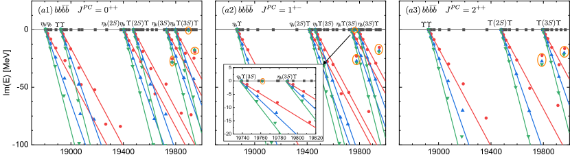
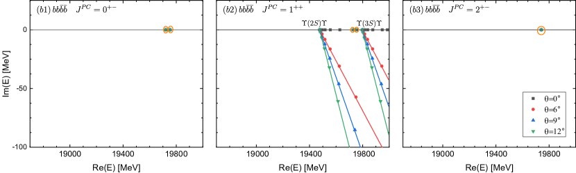
Figure 4: The complex energy eigenvalues of the $bb\bar{b}\bar{b}$ states with (a) “normal” and (b) “exotic” C-parities in the AP1 potential with varying $\theta$ in the CSM. The solid lines represent the continuum lines rotating along $\operatorname{Arg}(E)=-2\theta$. The zero-width states and resonances do not shift as $\theta$ changes and are highlighted by the orange circles.

III.3 Resonances with small widths

In our calculations, we obtain several extremely narrow resonant states with quantum numbers $J^{P}=1^{+}$ in both the $cc\bar{c}\bar{c}$ and $bb\bar{b}\bar{b}$ systems. Intuitively, one would assume that these states can decay into the di-quarkonium channels with the same quantum numbers and lower energies. However, the narrow widths of these states indicate that the two-body decay process is suppressed. The reasons for the suppression are given as follows.

The two-body decay width of the tetraquark state is proportional to the modulus square of the $T$-matrix element [91],

$$\Gamma_{F\rightarrow A+B}\propto\left|T_{F\rightarrow A+B}\right|^{2}=\left|\langle\psi_{AB}|\sum_{i<j=1}^{4}V_{ij}|\psi_{F}\rangle\right|^{2},$$ (18)

where $F$ denotes the tetraquark state and $A,B$ denote the final mesons. The potential $V_{ij}$ is given in Eq. (2), comprising the color magnetic term and spin-independent terms. In the fully heavy system, the color magnetic transition is suppressed by the heavy quark mass. The spin-independent terms contain the color factor $\boldsymbol{\lambda}_{i}\cdot\boldsymbol{\lambda}_{j}$, whose matrix elements are listed in Appendix A. It can be seen that $\sum_{i<j=1}^{4}\boldsymbol{\lambda}_{i}\cdot\boldsymbol{\lambda}_{j}$ is proportional to the identity operator and cannot induce transition between different color configurations. Color mixing via spin-independent terms can occur only when the coefficients of $\boldsymbol{\lambda}_{i}\cdot\boldsymbol{\lambda}_{j}$ are different. Roughly speaking, the magnitudes of color mixing matrix elements depend on the differences between various coefficients. From Tables 4,6,7,8, we can see that the different rms radii of the narrow resonances with $J^{P}=1^{+}$ are of the same order and the differences between them are rather small. Therefore, the color mixing matrix elements are suppressed in the system.

For the $1^{+-}$ $cc\bar{c}\bar{c}$ system, the state $T_{4c,1(-)}(6932)$ is a narrow resonance, whose dominant color-spin configuration is $[(c\bar{c})_{8_{c}}^{1}(c\bar{c})_{8_{c}}^{0}]_{1_{c}}^{1}$. On the other hand, the di-charmonium thresholds $\eta_{c}\psi$ have color-spin configuration $[(c\bar{c})_{1_{c}}^{1}(c\bar{c})_{1_{c}}^{0}]_{1_{c}}^{1}$. The transition between $T_{4c,1(-)}(6932)$ and the di-charmonium channels can only occur via color mixing, which is suppressed in the fully heavy system. For the $1^{++}$ $cc\bar{c}\bar{c}$ system, there are two types of narrow resonances. The first type $T_{4c,1(+)}(6896)$ and $T_{4c,1(+)}(7200)$ have dominant color-spin configuration $[(c\bar{c})_{8_{c}}^{1}(c\bar{c})_{8_{c}}^{1}]_{1_{c}}^{1}$ , while the second type $T_{4c,1(+)}(6939)$ and $T_{4c,1(+)}(7242)$ have dominant color-spin configuration $[(cc)_{\bar{3}_{c}}^{1}(\bar{c}\bar{c})_{3_{c}}^{1}]_{1_{c}}^{1}$. On the other hand, the di-charmonium thresholds $\Psi(2S)J/\psi$, $\Psi(3S)J/\Psi$ have color-spin configuration $[(c\bar{c})_{1_{c}}^{1}(c\bar{c})_{1_{c}}^{1}]_{1_{c}}^{1}$. The coupling between the first type of resonances and the di-charmonium channels is suppressed by the color mixing matrix elements. The spin configurations of the second type of resonances and the di-charmonium channels are orthogonal, which can be seen from the decomposition,

$${}^{1}= \frac{1}{\sqrt{2}}[(c_{1}\bar{c}_{3})^{1}(c_{2}\bar{c}_{4})^{0}]^{1}+$$ (19)

$$\frac{1}{\sqrt{2}}[(c_{1}\bar{c}_{3})^{0}(c_{2}\bar{c}_{4})^{1}]^{1}.$$

As a result, the coupling between them can only occur via the color magnetic term. Therefore the two-body decay widths of these two types of resonant states are both suppressed. For the $bb\bar{b}\bar{b}$ system, similar arguments can be used to account for the narrow widths of the states $T_{4b,1(-)}(19762)$, $T_{4b,1(+)}(19731)$ and $T_{4b,1(+)}(19748)$.

IV Summary

In summary, we calculate the mass spectrum of the S-wave fully heavy tetraquark systems with both “normal” $(J^{PC}=0^{++},1^{+-},2^{++})$ and “exotic” $(J^{PC}=0^{+-},1^{++},2^{+-})$ C-parities using three different quark potential models (AL1, AP1, BGS). The “exotic” C-parity systems refer to the ones that have no corresponding S-wave ground heavy quarkonia thresholds. We employ the Gaussian expansion method to solve the four-body Schrödinger equation, and the complex scaling method to distinguish resonant states from scattering states.

Our calculations show that the mass spectra in different quark models are in qualitative agreement. We obtain a series of resonant states with $J^{PC}=0^{++},1^{+-},2^{++}$ and $1^{++}$. Moreover, we obtain several zero-width states in the $0^{+-}$ and $2^{+-}$ systems, where S-wave di-quarkonium threshold does not exist. For the fully charmed system, we compare the theoretical results in the AP1 and BGS potentials with the experimental results in Fig. 5. We do not display the results in the AL1 potential since they are nearly the same as those in the AP1 potential. We find good candidates for the experimentally observed $X(6900)$ and $X(7200)$ in both the $0^{++}$ and $2^{++}$ systems. However, signals for the $X(6400)$ and $X(6600)$ are not seen in our calculations. Several resonant and zero-width fully charmed tetraquark states await to be found in the experiment. For the fully bottomed system, we summarize the theoretical results in the AP1 potential in Fig. 6. Resonant and zero-width fully bottomed tetraquark states are predicted in the mass region $(19.7,20.0)\,\mathrm{GeV}$.

By investigating the root mean square radii of the states, we find that most of the resonant and zero-width states have compact tetraquark configuration, except that the $X(7200)$ candidates $T_{4c,0(+)}(7173),T_{4c,2(+)}(7214)$ and the state $T_{4c,1(-)}(7191)$ may have molecular configurations. We also study the decay modes of the resonant and zero-width states. The resonant states can decay strongly to S-wave di-quarkonium thresholds while the zero-width states can only decay to P-wave quarkonia. Further study that considers the P-wave tetraquark systems is needed to better establish the properties of the $0^{+-}$ and $2^{+-}$ states.

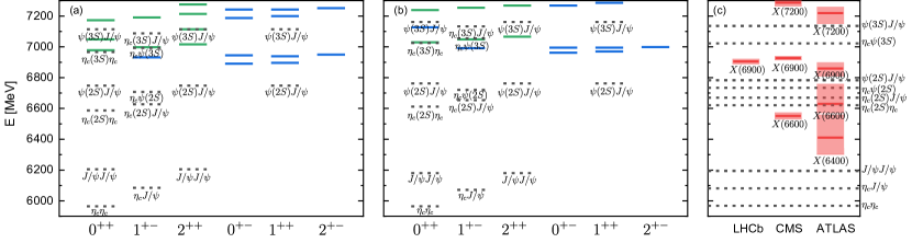
Figure 5: The mass spectrum of the S-wave $cc\bar{c}\bar{c}$ states in the (a) AP1, (b) BGS potential. The experimental results reported by LHCb (model I) [13], CMS (noninterference model) [14] and ATLAS (model A and $\alpha$) [15] are shown in Fig. (c). In Fig. (a) and (b), the green and blue lines represent the theoretical $cc\bar{c}\bar{c}$ states with widths larger and smaller than $1\,\mathrm{MeV}$, respectively. In Fig. (c), the red lines and the dashed areas represent the central masses and the uncertainties in the experiments, respectively. The dotted lines represent di-charmonium thresholds, whose experimental energies are taken from Ref. [87].

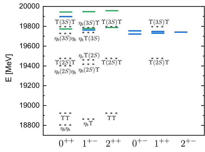
Figure 6: The mass spectrum of the S-wave $bb\bar{b}\bar{b}$ states in the AP1 potential. The green and blue lines represent the states with widths larger and smaller than $1\,\mathrm{MeV}$, respectively. The dotted lines represent di-charmonium thresholds, whose experimental energies are taken from Ref. [87].

Appendix A Color basis and color factors

The color basis of the tetraquark systems can be written in the diquark-antidiquark form,

$$\chi_{\bar{3}_{c}\otimes 3_{c}}=\left[\left(Q_{1}Q_{2}\right)_{\bar{3}_{c}}\left(\bar{Q}_{3}\bar{Q}_{4}\right)_{3_{c}}\right]_{1_{c}},$$ (20)

$$\chi_{6_{c}\otimes\bar{6}_{c}}=\left[\left(Q_{1}Q_{2}\right)_{6_{c}}\left(\bar{Q}_{3}\bar{Q}_{4}\right)_{\bar{6}_{c}}\right]_{1_{c}},$$

or in two sets of dimeson form,

$$\chi^{a}_{1_{c}\otimes 1_{c}}=\left[\left(Q_{1}\bar{Q}_{3}\right)_{1_{c}}\left(Q_{2}\bar{Q}_{4}\right)_{1_{c}}\right]_{1_{c}},$$ (21)

$$\chi^{a}_{8_{c}\otimes 8_{c}}=\left[\left(Q_{1}\bar{Q}_{3}\right)_{8_{c}}\left(Q_{2}\bar{Q}_{4}\right)_{8_{c}}\right]_{1_{c}},$$

$$\chi^{b}_{1_{c}\otimes 1_{c}}=\left[\left(Q_{1}\bar{Q}_{4}\right)_{1_{c}}\left(Q_{2}\bar{Q}_{3}\right)_{1_{c}}\right]_{1_{c}},$$ (22)

$$\chi^{b}_{8_{c}\otimes 8_{c}}=\left[\left(Q_{1}\bar{Q}_{4}\right)_{8_{c}}\left(Q_{2}\bar{Q}_{3}\right)_{8_{c}}\right]_{1_{c}}.$$

Each of these forms constitute a complete and orthogonal color basis for the tetraquark systems. The transformation between different sets of bases is given by

$$\chi^{a}_{1_{c}\otimes 1_{c}}=\frac{1}{\sqrt{3}}(\chi_{\bar{3}_{c}\otimes 3_{c}}+\sqrt{2}\chi_{6_{c}\otimes\bar{6}_{c}}),$$ (23)

$$\chi^{a}_{8_{c}\otimes 8_{c}}=\frac{1}{\sqrt{3}}(-\sqrt{2}\chi_{\bar{3}_{c}\otimes 3_{c}}+\chi_{6_{c}\otimes\bar{6}_{c}}),$$

$$\chi^{b}_{1_{c}\otimes 1_{c}}=\frac{1}{\sqrt{3}}(-\chi_{\bar{3}_{c}\otimes 3_{c}}+\sqrt{2}\chi_{6_{c}\otimes\bar{6}_{c}}),$$

$$\chi^{b}_{8_{c}\otimes 8_{c}}=\frac{1}{\sqrt{3}}(\sqrt{2}\chi_{\bar{3}_{c}\otimes 3_{c}}+\chi_{6_{c}\otimes\bar{6}_{c}}).$$

It is equivalent to use Eqs. (20), (21) or (22) as the color basis in the calculations. The matrix elements for the color factor $\boldsymbol{\lambda}_{i}\cdot\boldsymbol{\lambda}_{j}$ in the diquark-antidiquark color basis (20) are listed in Table 9. From the last column we can see that $\sum_{i<j=1}^{4}\boldsymbol{\lambda}_{i}\cdot\boldsymbol{\lambda}_{j}$ is actually proportional to the identity operator.

Table 9: Color factor matrix elements $\langle\chi_{c}|\boldsymbol{\lambda}_{i}\cdot\boldsymbol{\lambda}_{j}|\chi_{c}^{\prime}\rangle$ in the color basis (20).

$\langle\chi_{c}|\bm{\lambda}_{i}\cdot\bm{\lambda}_{j}|\chi_{c}^{\prime}\rangle$	$\bm{\lambda}_{1}\cdot\bm{\lambda}_{2}$	$\bm{\lambda}_{3}\cdot\bm{\lambda}_{4}$	$\bm{\lambda}_{1}\cdot\bm{\lambda}_{3}$	$\bm{\lambda}_{1}\cdot\bm{\lambda}_{4}$	$\bm{\lambda}_{2}\cdot\bm{\lambda}_{3}$	$\bm{\lambda}_{2}\cdot\bm{\lambda}_{4}$	$\sum_{i<j=1}^{4}\boldsymbol{\lambda}_{i}\cdot\boldsymbol{\lambda}_{j}$
$\langle\chi_{\bar{3}_{c}\otimes 3_{c}}|\bm{\lambda}_{i}\cdot\bm{\lambda}_{j}|\chi_{\bar{3}_{c}\otimes 3_{c}}\rangle$	$-\frac{8}{3}$	$-\frac{8}{3}$	$-\frac{4}{3}$	$-\frac{4}{3}$	$-\frac{4}{3}$	$-\frac{4}{3}$	-$\frac{32}{3}$
$\langle\chi_{6_{c}\otimes\bar{6}_{c}}|\bm{\lambda}_{i}\cdot\bm{\lambda}_{j}|\chi_{6_{c}\otimes\bar{6}_{c}}\rangle$	$\frac{4}{3}$	$\frac{4}{3}$	$-\frac{10}{3}$	$-\frac{10}{3}$	$-\frac{10}{3}$	$-\frac{10}{3}$	-$\frac{32}{3}$
$\langle\chi_{\bar{3}_{c}\otimes 3_{c}}|\bm{\lambda}_{i}\cdot\bm{\lambda}_{j}|\chi_{6_{c}\otimes\bar{6}_{c}}\rangle$	$0$	$0$	$-2\sqrt{2}$	$2\sqrt{2}$	$2\sqrt{2}$	$-2\sqrt{2}$	0

Appendix B Basis functions with definite C-parity

Under charge conjugation, the transformation behaviour of the basis functions is shown in Eqs. (11)-(13). Using the linear superposition of the original basis functions, we can construct a new set of basis with definite C-parity and decompose the Hilbert space $\mathcal{H}$ into positive and negative C-parity subspaces $\mathcal{H}_{\pm}$. The basis functions of $\mathcal{H}_{\pm}$ with different quantum numbers and satisfying the antisymmetrization of identical particles are explicitly listed in the following.

• $J^{PC}=0^{++}$

  $$\chi^{0}_{\bar{3}_{c}\otimes 3_{c},1,1}[\Phi^{(\rm{c})}_{n_{1},n_{2}}+\Phi^{(\rm{c})}_{n_{2},n_{1}}],$$ (24)

  $$\chi^{0}_{6_{c}\otimes\bar{6}_{c},0,0}[\Phi^{(\rm{c})}_{n_{1},n_{2}}+\Phi^{(\rm{c})}_{n_{2},n_{1}}],$$ (25)

  $$\chi^{0}_{\bar{3}_{c}\otimes 3_{c},1,1}[\Phi^{(\rm{a})}_{n_{1},n_{2}}+\Phi^{(\rm{b})}_{n_{1},n_{2}}+\Phi^{(\rm{a})}_{n_{2},n_{1}}+\Phi^{(\rm{b})}_{n_{2},n_{1}}],$$ (26)

  $$\chi^{0}_{6_{c}\otimes\bar{6}_{c},0,0}[\Phi^{(\rm{a})}_{n_{1},n_{2}}+\Phi^{(\rm{b})}_{n_{1},n_{2}}+\Phi^{(\rm{a})}_{n_{2},n_{1}}+\Phi^{(\rm{b})}_{n_{2},n_{1}}],$$ (27)

  $$\chi^{0}_{\bar{3}_{c}\otimes 3_{c},0,0}[\Phi^{(\rm{a})}_{n_{1},n_{2}}-\Phi^{(\rm{b})}_{n_{1},n_{2}}+\Phi^{(\rm{a})}_{n_{2},n_{1}}-\Phi^{(\rm{b})}_{n_{2},n_{1}}],$$ (28)

  $$\chi^{0}_{6_{c}\otimes\bar{6}_{c},1,1}[\Phi^{(\rm{a})}_{n_{1},n_{2}}-\Phi^{(\rm{b})}_{n_{1},n_{2}}+\Phi^{(\rm{a})}_{n_{2},n_{1}}-\Phi^{(\rm{b})}_{n_{2},n_{1}}],$$ (29)

• $J^{PC}=0^{+-}$

  $$\chi^{0}_{\bar{3}_{c}\otimes 3_{c},1,1}[\Phi^{(\rm{c})}_{n_{1},n_{2}}-\Phi^{(\rm{c})}_{n_{2},n_{1}}],$$ (30)

  $$\chi^{0}_{6_{c}\otimes\bar{6}_{c},0,0}[\Phi^{(\rm{c})}_{n_{1},n_{2}}-\Phi^{(\rm{c})}_{n_{2},n_{1}}],$$ (31)

• $J^{PC}=1^{++}$

  $$\chi^{1}_{\bar{3}_{c}\otimes 3_{c},1,1}[\Phi^{(\rm{c})}_{n_{1},n_{2}}-\Phi^{(\rm{c})}_{n_{2},n_{1}}],$$ (32)

  $$\chi^{1}_{\bar{3}_{c}\otimes 3_{c},1,0}[\Phi^{(\rm{a})}_{n_{1},n_{2}}-\Phi^{(\rm{b})}_{n_{1},n_{2}}-\Phi^{(\rm{a})}_{n_{2},n_{1}}+\Phi^{(\rm{b})}_{n_{2},n_{1}}]$$

  $$+ \chi^{1}_{\bar{3}_{c}\otimes 3_{c},0,1}[\Phi^{(\rm{a})}_{n_{1},n_{2}}+\Phi^{(\rm{b})}_{n_{1},n_{2}}-\Phi^{(\rm{a})}_{n_{2},n_{1}}-\Phi^{(\rm{b})}_{n_{2},n_{1}}],$$ (33)

  $$\chi^{1}_{6_{c}\otimes\bar{6}_{c},0,1}[\Phi^{(\rm{a})}_{n_{1},n_{2}}-\Phi^{(\rm{b})}_{n_{1},n_{2}}-\Phi^{(\rm{a})}_{n_{2},n_{1}}+\Phi^{(\rm{b})}_{n_{2},n_{1}}]$$

  $$+ \chi^{1}_{6_{c}\otimes\bar{6}_{c},1,0}[\Phi^{(\rm{a})}_{n_{1},n_{2}}+\Phi^{(\rm{b})}_{n_{1},n_{2}}-\Phi^{(\rm{a})}_{n_{2},n_{1}}-\Phi^{(\rm{b})}_{n_{2},n_{1}}],$$ (34)

• $J^{PC}=1^{+-}$

  $$\chi^{1}_{\bar{3}_{c}\otimes 3_{c},1,1}[\Phi^{(\rm{c})}_{n_{1},n_{2}}+\Phi^{(\rm{c})}_{n_{2},n_{1}}],$$ (35)

  $$\chi^{1}_{\bar{3}_{c}\otimes 3_{c},1,1}[\Phi^{(\rm{a})}_{n_{1},n_{2}}+\Phi^{(\rm{b})}_{n_{1},n_{2}}+\Phi^{(\rm{a})}_{n_{2},n_{1}}+\Phi^{(\rm{b})}_{n_{2},n_{1}}],$$ (36)

  $$\chi^{1}_{6_{c}\otimes\bar{6}_{c},1,1}[\Phi^{(\rm{a})}_{n_{1},n_{2}}-\Phi^{(\rm{b})}_{n_{1},n_{2}}+\Phi^{(\rm{a})}_{n_{2},n_{1}}-\Phi^{(\rm{b})}_{n_{2},n_{1}}],$$ (37)

  $$\chi^{1}_{\bar{3}_{c}\otimes 3_{c},1,0}[\Phi^{(\rm{a})}_{n_{1},n_{2}}-\Phi^{(\rm{b})}_{n_{1},n_{2}}-\Phi^{(\rm{a})}_{n_{2},n_{1}}+\Phi^{(\rm{b})}_{n_{2},n_{1}}]$$

  $$- \chi^{1}_{\bar{3}_{c}\otimes 3_{c},0,1}[\Phi^{(\rm{a})}_{n_{1},n_{2}}+\Phi^{(\rm{b})}_{n_{1},n_{2}}-\Phi^{(\rm{a})}_{n_{2},n_{1}}-\Phi^{(\rm{b})}_{n_{2},n_{1}}],$$ (38)

  $$\chi^{1}_{6_{c}\otimes\bar{6}_{c},0,1}[\Phi^{(\rm{a})}_{n_{1},n_{2}}-\Phi^{(\rm{b})}_{n_{1},n_{2}}-\Phi^{(\rm{a})}_{n_{2},n_{1}}+\Phi^{(\rm{b})}_{n_{2},n_{1}}]$$

  $$- \chi^{1}_{6_{c}\otimes\bar{6}_{c},1,0}[\Phi^{(\rm{a})}_{n_{1},n_{2}}+\Phi^{(\rm{b})}_{n_{1},n_{2}}-\Phi^{(\rm{a})}_{n_{2},n_{1}}-\Phi^{(\rm{b})}_{n_{2},n_{1}}],$$ (39)

• $J^{PC}=2^{++}$

  $$\chi^{2}_{\bar{3}_{c}\otimes 3_{c},1,1}[\Phi^{(\rm{c})}_{n_{1},n_{2}}+\Phi^{(\rm{c})}_{n_{2},n_{1}}],$$ (40)

  $$\chi^{2}_{\bar{3}_{c}\otimes 3_{c},1,1}[\Phi^{(\rm{a})}_{n_{1},n_{2}}+\Phi^{(\rm{b})}_{n_{1},n_{2}}+\Phi^{(\rm{a})}_{n_{2},n_{1}}+\Phi^{(\rm{b})}_{n_{2},n_{1}}],$$ (41)

  $$\chi^{2}_{6_{c}\otimes\bar{6}_{c},1,1}[\Phi^{(\rm{a})}_{n_{1},n_{2}}-\Phi^{(\rm{b})}_{n_{1},n_{2}}+\Phi^{(\rm{a})}_{n_{2},n_{1}}-\Phi^{(\rm{b})}_{n_{2},n_{1}}],$$ (42)

• $J^{PC}=2^{+-}$

  $$\chi^{2}_{\bar{3}_{c}\otimes 3_{c},1,1}[\Phi^{(\rm{c})}_{n_{1},n_{2}}-\Phi^{(\rm{c})}_{n_{2},n_{1}}],$$ (43)

where $\chi_{c_{1}\otimes c_{2},s_{1},s_{2}}^{J}$ is the color-spin wave function, and $\Phi^{(\rm{jac})}_{n_{1},n_{2}}\equiv\Phi^{(\rm{jac})}_{n_{1},n_{2},n_{3}}$ is the S-wave Gaussian spatial wave function. The detail expression for the wave functions can be found in Eqs. (6) and (8).

We can see that the S-wave fully heavy tetraquark states with $J^{PC}=0^{+-}$ and $2^{+-}$ contain only diquark-antidiquark configuration $\Phi^{(\rm{c})}_{n_{1},n_{2},n_{3}}$ and exclude dimeson configuration $\Phi^{(\rm{a})}_{n_{1},n_{2},n_{3}}$, $\Phi^{(\rm{b})}_{n_{1},n_{2},n_{3}}$, which arises from the fact that S-wave dimeson systems cannot have such quantum numbers. It should be noted that the minus sign in Eqs. (30), (31) and (43) demands that the radial excitation of the diquark and the antidiquark must be different, therefore the $0^{+-}$ or $2^{+-}$ tetraquark state is not a particle-antiparticle pair and one cannot simply calculate the C-parity as $C=(-1)^{L+S}=+1$.

References

- Choi et al. [2003] S. K. Choi et al. (Belle), Observation of a narrow charmonium-like state in exclusive decays, Phys. Rev. Lett. 91, 262001 (2003), arXiv:hep-ex/0309032 .
- Chen et al. [2016] H.-X. Chen, W. Chen, X. Liu, and S.-L. Zhu, The hidden-charm pentaquark and tetraquark states, Phys. Rept. 639, 1 (2016), arXiv:1601.02092 [hep-ph] .
- Esposito et al. [2017] A. Esposito, A. Pilloni, and A. D. Polosa, Multiquark Resonances, Phys. Rept. 668, 1 (2017), arXiv:1611.07920 [hep-ph] .
- Hosaka et al. [2016] A. Hosaka, T. Iijima, K. Miyabayashi, Y. Sakai, and S. Yasui, Exotic hadrons with heavy flavors: X, Y, Z, and related states, PTEP 2016, 062C01 (2016), arXiv:1603.09229 [hep-ph] .
- Lebed et al. [2017] R. F. Lebed, R. E. Mitchell, and E. S. Swanson, Heavy-Quark QCD Exotica, Prog. Part. Nucl. Phys. 93, 143 (2017), arXiv:1610.04528 [hep-ph] .
- Guo et al. [2018] F.-K. Guo, C. Hanhart, U.-G. Meißner, Q. Wang, Q. Zhao, and B.-S. Zou, Hadronic molecules, Rev. Mod. Phys. 90, 015004 (2018), [Erratum: Rev.Mod.Phys. 94, 029901 (2022)], arXiv:1705.00141 [hep-ph] .
- Ali et al. [2017] A. Ali, J. S. Lange, and S. Stone, Exotics: Heavy Pentaquarks and Tetraquarks, Prog. Part. Nucl. Phys. 97, 123 (2017), arXiv:1706.00610 [hep-ph] .
- Brambilla et al. [2020] N. Brambilla, S. Eidelman, C. Hanhart, A. Nefediev, C.-P. Shen, C. E. Thomas, A. Vairo, and C.-Z. Yuan, The states: experimental and theoretical status and perspectives, Phys. Rept. 873, 1 (2020), arXiv:1907.07583 [hep-ex] .
- Liu et al. [2019] Y.-R. Liu, H.-X. Chen, W. Chen, X. Liu, and S.-L. Zhu, Pentaquark and Tetraquark states, Prog. Part. Nucl. Phys. 107, 237 (2019), arXiv:1903.11976 [hep-ph] .
- Meng et al. [2023a] L. Meng, B. Wang, G.-J. Wang, and S.-L. Zhu, Chiral perturbation theory for heavy hadrons and chiral effective field theory for heavy hadronic molecules, Phys. Rept. 1019, 1 (2023a), arXiv:2204.08716 [hep-ph] .
- Mai et al. [2023] M. Mai, U.-G. Meißner, and C. Urbach, Towards a theory of hadron resonances, Phys. Rept. 1001, 1 (2023), arXiv:2206.01477 [hep-ph] .
- Chen et al. [2023] H.-X. Chen, W. Chen, X. Liu, Y.-R. Liu, and S.-L. Zhu, An updated review of the new hadron states, Rept. Prog. Phys. 86, 026201 (2023), arXiv:2204.02649 [hep-ph] .
- Aaij et al. [2020] R. Aaij et al. (LHCb), Observation of structure in the -pair mass spectrum, Sci. Bull. 65, 1983 (2020), arXiv:2006.16957 [hep-ex] .
- Hayrapetyan et al. [2023] A. Hayrapetyan et al. (CMS), Observation of new structure in the J/J/ mass spectrum in proton-proton collisions at = 13 TeV, (2023), arXiv:2306.07164 [hep-ex] .
- Aad et al. [2023] G. Aad et al. (ATLAS), Observation of an Excess of Dicharmonium Events in the Four-Muon Final State with the ATLAS Detector, Phys. Rev. Lett. 131, 151902 (2023), arXiv:2304.08962 [hep-ex] .
- Iwasaki [1975] Y. Iwasaki, A Possible Model for New Resonances-Exotics and Hidden Charm, Prog. Theor. Phys. 54, 492 (1975).
- Chao [1981] K.-T. Chao, The (cc) - () (Diquark - Anti-Diquark) States in Annihilation, Z. Phys. C 7, 317 (1981).
- Ader et al. [1982] J. P. Ader, J. M. Richard, and P. Taxil, DO NARROW HEAVY MULTI - QUARK STATES EXIST?, Phys. Rev. D 25, 2370 (1982).
- Zouzou et al. [1986] S. Zouzou, B. Silvestre-Brac, C. Gignoux, and J. M. Richard, FOUR QUARK BOUND STATES, Z. Phys. C 30, 457 (1986).
- Heller and Tjon [1987] L. Heller and J. A. Tjon, On the Existence of Stable Dimesons, Phys. Rev. D 35, 969 (1987).
- Silvestre-Brac [1992] B. Silvestre-Brac, Systematics of Q**2 (anti-Q**2) systems with a chromomagnetic interaction, Phys. Rev. D 46, 2179 (1992).
- Silvestre-Brac and Semay [1993] B. Silvestre-Brac and C. Semay, Spectrum and decay properties of diquonia, Z. Phys. C 59, 457 (1993).
- Wu et al. [2018] J. Wu, Y.-R. Liu, K. Chen, X. Liu, and S.-L. Zhu, Heavy-flavored tetraquark states with the configuration, Phys. Rev. D 97, 094015 (2018), arXiv:1605.01134 [hep-ph] .
- Chen et al. [2017] W. Chen, H.-X. Chen, X. Liu, T. G. Steele, and S.-L. Zhu, Hunting for exotic doubly hidden-charm/bottom tetraquark states, Phys. Lett. B 773, 247 (2017), arXiv:1605.01647 [hep-ph] .
- Wang et al. [2019] G.-J. Wang, L. Meng, and S.-L. Zhu, Spectrum of the fully-heavy tetraquark state , Phys. Rev. D 100, 096013 (2019), arXiv:1907.05177 [hep-ph] .
- Bedolla et al. [2020] M. A. Bedolla, J. Ferretti, C. D. Roberts, and E. Santopinto, Spectrum of fully-heavy tetraquarks from a diquark+antidiquark perspective, Eur. Phys. J. C 80, 1004 (2020), arXiv:1911.00960 [hep-ph] .
- Deng et al. [2021] C. Deng, H. Chen, and J. Ping, Towards the understanding of fully-heavy tetraquark states from various models, Phys. Rev. D 103, 014001 (2021), arXiv:2003.05154 [hep-ph] .
- liu et al. [2020] M.-S. liu, F.-X. Liu, X.-H. Zhong, and Q. Zhao, Full-heavy tetraquark states and their evidences in the LHCb di- spectrum, (2020), arXiv:2006.11952 [hep-ph] .
- Jin et al. [2020] X. Jin, Y. Xue, H. Huang, and J. Ping, Full-heavy tetraquarks in constituent quark models, Eur. Phys. J. C 80, 1083 (2020), arXiv:2006.13745 [hep-ph] .
- Lü et al. [2020] Q.-F. Lü, D.-Y. Chen, and Y.-B. Dong, Masses of fully heavy tetraquarks in an extended relativized quark model, Eur. Phys. J. C 80, 871 (2020), arXiv:2006.14445 [hep-ph] .
- Chen et al. [2020] H.-X. Chen, W. Chen, X. Liu, and S.-L. Zhu, Strong decays of fully-charm tetraquarks into di-charmonia, Sci. Bull. 65, 1994 (2020), arXiv:2006.16027 [hep-ph] .
- Wang et al. [2020] X.-Y. Wang, Q.-Y. Lin, H. Xu, Y.-P. Xie, Y. Huang, and X. Chen, Discovery potential for the LHCb fully-charm tetraquark state via annihilation reaction, Phys. Rev. D 102, 116014 (2020), arXiv:2007.09697 [hep-ph] .
- Albuquerque et al. [2020] R. M. Albuquerque, S. Narison, A. Rabemananjara, D. Rabetiarivony, and G. Randriamanatrika, Doubly-hidden scalar heavy molecules and tetraquarks states from QCD at NLO, Phys. Rev. D 102, 094001 (2020), arXiv:2008.01569 [hep-ph] .
- Giron and Lebed [2020] J. F. Giron and R. F. Lebed, Simple spectrum of states in the dynamical diquark model, Phys. Rev. D 102, 074003 (2020), arXiv:2008.01631 [hep-ph] .
- Wang et al. [2021a] J.-Z. Wang, D.-Y. Chen, X. Liu, and T. Matsuki, Producing fully charm structures in the -pair invariant mass spectrum, Phys. Rev. D 103, 071503 (2021a), arXiv:2008.07430 [hep-ph] .
- Dong et al. [2021a] X.-K. Dong, V. Baru, F.-K. Guo, C. Hanhart, and A. Nefediev, Coupled-Channel Interpretation of the LHCb Double- Spectrum and Hints of a New State Near the Threshold, Phys. Rev. Lett. 126, 132001 (2021a), [Erratum: Phys.Rev.Lett. 127, 119901 (2021)], arXiv:2009.07795 [hep-ph] .
- Zhang and Ma [2020] H.-F. Zhang and Y.-Q. Ma, Exploring the di- resonances based on \itab initio perturbative QCD, (2020), arXiv:2009.08376 [hep-ph] .
- Zhao et al. [2020] J. Zhao, S. Shi, and P. Zhuang, Fully-heavy tetraquarks in a strongly interacting medium, Phys. Rev. D 102, 114001 (2020), arXiv:2009.10319 [hep-ph] .
- Gordillo et al. [2020] M. C. Gordillo, F. De Soto, and J. Segovia, Diffusion Monte Carlo calculations of fully-heavy multiquark bound states, Phys. Rev. D 102, 114007 (2020), arXiv:2009.11889 [hep-ph] .
- Weng et al. [2021] X.-Z. Weng, X.-L. Chen, W.-Z. Deng, and S.-L. Zhu, Systematics of fully heavy tetraquarks, Phys. Rev. D 103, 034001 (2021), arXiv:2010.05163 [hep-ph] .
- Zhang [2021] J.-R. Zhang, fully-charmed tetraquark states, Phys. Rev. D 103, 014018 (2021), arXiv:2010.07719 [hep-ph] .
- Guo and Oller [2021] Z.-H. Guo and J. A. Oller, Insights into the inner structures of the fully charmed tetraquark state , Phys. Rev. D 103, 034024 (2021), arXiv:2011.00978 [hep-ph] .
- Gong et al. [2022a] C. Gong, M.-C. Du, Q. Zhao, X.-H. Zhong, and B. Zhou, Nature of X(6900) and its production mechanism at LHCb, Phys. Lett. B 824, 136794 (2022a), arXiv:2011.11374 [hep-ph] .
- Wan and Qiao [2021] B.-D. Wan and C.-F. Qiao, Gluonic tetracharm configuration of , Phys. Lett. B 817, 136339 (2021), arXiv:2012.00454 [hep-ph] .
- Dosch et al. [2021] H. G. Dosch, S. J. Brodsky, G. F. de Téramond, M. Nielsen, and L. Zou, Exotic states in a holographic theory, Nucl. Part. Phys. Proc. 312-317, 135 (2021), arXiv:2012.02496 [hep-ph] .
- Yang et al. [2021a] B.-C. Yang, L. Tang, and C.-F. Qiao, Scalar fully-heavy tetraquark states in QCD sum rules, Eur. Phys. J. C 81, 324 (2021a), arXiv:2012.04463 [hep-ph] .
- Huang et al. [2021] G. Huang, J. Zhao, and P. Zhuang, Pair structure of heavy tetraquark systems, Phys. Rev. D 103, 054014 (2021), arXiv:2012.14845 [hep-ph] .
- Zhao et al. [2021] Z. Zhao, K. Xu, A. Kaewsnod, X. Liu, A. Limphirat, and Y. Yan, Study of charmoniumlike and fully-charm tetraquark spectroscopy, Phys. Rev. D 103, 116027 (2021), arXiv:2012.15554 [hep-ph] .
- Hughes [2021] C. Hughes, Theory Overview of Heavy Exotic Spectroscopy, PoS BEAUTY2020, 044 (2021), arXiv:2101.08241 [hep-ph] .
- Faustov et al. [2021] R. N. Faustov, V. O. Galkin, and E. M. Savchenko, Heavy tetraquarks in the relativistic quark model, Universe 7, 94 (2021), arXiv:2103.01763 [hep-ph] .
- Ke et al. [2021] H.-W. Ke, X. Han, X.-H. Liu, and Y.-L. Shi, Tetraquark state and the interaction between diquark and antidiquark, Eur. Phys. J. C 81, 427 (2021), arXiv:2103.13140 [hep-ph] .
- Liang et al. [2021] Z.-R. Liang, X.-Y. Wu, and D.-L. Yao, Hunting for states in the recent LHCb di-J/ invariant mass spectrum, Phys. Rev. D 104, 034034 (2021), arXiv:2104.08589 [hep-ph] .
- Yang et al. [2021b] G. Yang, J. Ping, and J. Segovia, Exotic resonances of fully-heavy tetraquarks in a lattice-QCD insipired quark model, Phys. Rev. D 104, 014006 (2021b), arXiv:2104.08814 [hep-ph] .
- Mutuk [2021] H. Mutuk, Nonrelativistic treatment of fully-heavy tetraquarks as diquark-antidiquark states, Eur. Phys. J. C 81, 367 (2021), arXiv:2104.11823 [hep-ph] .
- Li et al. [2021] Q. Li, C.-H. Chang, G.-L. Wang, and T. Wang, Mass spectra and wave functions of TQQQ¯Q¯ tetraquarks, Phys. Rev. D 104, 014018 (2021), arXiv:2104.12372 [hep-ph] .
- Wang et al. [2021b] G.-J. Wang, L. Meng, M. Oka, and S.-L. Zhu, Higher fully charmed tetraquarks: Radial excitations and P-wave states, Phys. Rev. D 104, 036016 (2021b), arXiv:2105.13109 [hep-ph] .
- Dong et al. [2021b] X.-K. Dong, V. Baru, F.-K. Guo, C. Hanhart, A. Nefediev, and B.-S. Zou, Is the existence of a J/J/ bound state plausible?, Sci. Bull. 66, 2462 (2021b), arXiv:2107.03946 [hep-ph] .
- Wang et al. [2021c] Q.-N. Wang, Z.-Y. Yang, and W. Chen, Exotic fully-heavy tetraquark states in color configuration, Phys. Rev. D 104, 114037 (2021c), arXiv:2109.08091 [hep-ph] .
- Liu et al. [2021] F.-X. Liu, M.-S. Liu, X.-H. Zhong, and Q. Zhao, Higher mass spectra of the fully-charmed and fully-bottom tetraquarks, Phys. Rev. D 104, 116029 (2021), arXiv:2110.09052 [hep-ph] .
- Zhuang et al. [2022] Z. Zhuang, Y. Zhang, Y. Ma, and Q. Wang, Lineshape of the compact fully heavy tetraquark, Phys. Rev. D 105, 054026 (2022), arXiv:2111.14028 [hep-ph] .
- Asadi and Boroun [2022] Z. Asadi and G. R. Boroun, Masses of fully heavy tetraquark states from a four-quark static potential model, Phys. Rev. D 105, 014006 (2022), arXiv:2112.11028 [hep-ph] .
- Kuang et al. [2022] Z. Kuang, K. Serafin, X. Zhao, and J. P. Vary (BLFQ), All-charm tetraquark in front form dynamics, Phys. Rev. D 105, 094028 (2022), arXiv:2201.06428 [hep-ph] .
- Gong et al. [2022b] C. Gong, M.-C. Du, and Q. Zhao, Pseudoscalar charmonium pair interactions via the Pomeron exchange mechanism, Phys. Rev. D 106, 054011 (2022b), arXiv:2206.13867 [hep-ph] .
- Wang and Liu [2022] J.-Z. Wang and X. Liu, Improved understanding of the peaking phenomenon existing in the new di-J/ invariant mass spectrum from the CMS Collaboration, Phys. Rev. D 106, 054015 (2022), arXiv:2207.04893 [hep-ph] .
- Zhou et al. [2022] Q. Zhou, D. Guo, S.-Q. Kuang, Q.-H. Yang, and L.-Y. Dai, Nature of the X(6900) in partial wave decomposition of J/J/ scattering, Phys. Rev. D 106, L111502 (2022), arXiv:2207.07537 [hep-ph] .
- Chen et al. [2022] H.-X. Chen, Y.-X. Yan, and W. Chen, Decay behaviors of the fully bottom and fully charm tetraquark states, Phys. Rev. D 106, 094019 (2022), arXiv:2207.08593 [hep-ph] .
- An et al. [2023] H.-T. An, S.-Q. Luo, Z.-W. Liu, and X. Liu, Spectroscopic behavior of fully heavy tetraquarks, Eur. Phys. J. C 83, 740 (2023), arXiv:2208.03899 [hep-ph] .
- Wang et al. [2022] G.-J. Wang, Q. Meng, and M. Oka, S-wave fully charmed tetraquark resonant states, Phys. Rev. D 106, 096005 (2022), arXiv:2208.07292 [hep-ph] .
- Niu et al. [2022] P.-Y. Niu, E. Wang, Q. Wang, and S. Yang, Determine the quantum numbers of from photon-photon fusion in ultra-peripheral heavy ion collisions, (2022), arXiv:2209.01924 [hep-ph] .
- Zhang et al. [2022] J. Zhang, J.-B. Wang, G. Li, C.-S. An, C.-R. Deng, and J.-J. Xie, Spectrum of the S-wave fully-heavy tetraquark states, Eur. Phys. J. C 82, 1126 (2022), arXiv:2209.13856 [hep-ph] .
- Yu et al. [2023] G.-L. Yu, Z.-Y. Li, Z.-G. Wang, J. Lu, and M. Yan, The S- and P-wave fully charmed tetraquark states and their radial excitations, Eur. Phys. J. C 83, 416 (2023), arXiv:2212.14339 [hep-ph] .
- Ortega et al. [2023] P. G. Ortega, D. R. Entem, and F. Fernández, Exploring T tetraquark candidates in a coupled-channels formalism, Phys. Rev. D 108, 094023 (2023), arXiv:2307.00532 [hep-ph] .
- Wang et al. [2023] G.-J. Wang, M. Oka, and D. Jido, Quark confinement for multiquark systems: Application to fully charmed tetraquarks, Phys. Rev. D 108, L071501 (2023).
- Sang et al. [2023] W.-L. Sang, T. Wang, Y.-D. Zhang, and F. Feng, Electromagnetic and hadronic decay of fully heavy tetraquark, (2023), arXiv:2307.16150 [hep-ph] .
- Galkin and Savchenko [2023] V. O. Galkin and E. M. Savchenko, Relativistic description of asymmetric fully heavy tetraquarks in the diquark-antidiquark model, (2023), arXiv:2310.20247 [hep-ph] .
- Anwar and Burns [2023] M. N. Anwar and T. J. Burns, Structure of tetraquarks and interpretation of LHC states, (2023), arXiv:2311.15853 [hep-ph] .
- Ma et al. [2023a] Y. Ma, L. Meng, Y.-K. Chen, and S.-L. Zhu, Ground state baryons in the flux-tube three-body confinement model using diffusion Monte Carlo, Phys. Rev. D 107, 054035 (2023a), arXiv:2211.09021 [hep-ph] .
- Ma et al. [2023b] Y. Ma, L. Meng, Y.-K. Chen, and S.-L. Zhu, Doubly heavy tetraquark states in the constituent quark model using diffusion Monte Carlo method, (2023b), arXiv:2309.17068 [hep-ph] .
- Meng et al. [2023b] L. Meng, Y.-K. Chen, Y. Ma, and S.-L. Zhu, Tetraquark bound states in constituent quark models: Benchmark test calculations, Phys. Rev. D 108, 114016 (2023b), arXiv:2310.13354 [hep-ph] .
- Aguilar and Combes [1971] J. Aguilar and J. M. Combes, A class of analytic perturbations for one-body schroedinger hamiltonians, Commun. Math. Phys. 22, 269 (1971).
- Balslev and Combes [1971] E. Balslev and J. M. Combes, Spectral properties of many-body schroedinger operators with dilatation-analytic interactions, Commun. Math. Phys. 22, 280 (1971).
- Aoyama et al. [2006] S. Aoyama, T. Myo, K. Katō, and K. Ikeda, The complex scaling method for many-body resonances and its applications to three-body resonances, Progress of theoretical physics 116, 1 (2006).
- Chen et al. [2024] Y.-K. Chen, W.-L. Wu, L. Meng, and S.-L. Zhu, Unified description of the Qsq¯q¯ molecular bound states, molecular resonances, and compact tetraquark states in the quark potential model, Phys. Rev. D 109, 014010 (2024), arXiv:2310.14597 [hep-ph] .
- Semay and Silvestre-Brac [1994] C. Semay and B. Silvestre-Brac, Diquonia and potential models, Z. Phys. C 61, 271 (1994).
- Silvestre-Brac [1996] B. Silvestre-Brac, Spectrum and static properties of heavy baryons, Few Body Syst. 20, 1 (1996).
- Barnes et al. [2005] T. Barnes, S. Godfrey, and E. S. Swanson, Higher charmonia, Phys. Rev. D 72, 054026 (2005), arXiv:hep-ph/0505002 .
- Workman et al. [2022] R. L. Workman et al. (Particle Data Group), Review of Particle Physics, PTEP 2022, 083C01 (2022).
- Hiyama et al. [2003] E. Hiyama, Y. Kino, and M. Kamimura, Gaussian expansion method for few-body systems, Progress in Particle and Nuclear Physics 51, 223 (2003).
- Romo [1968] W. J. Romo, Inner product for resonant states and shell-model applications, Nuclear Physics A 116, 617 (1968).
- Homma et al. [1997] M. Homma, T. Myo, and K. Katō, Matrix Elements of Physical Quantities Associated with Resonance States, Progress of Theoretical Physics 97, 561 (1997), https://academic.oup.com/ptp/article-pdf/97/4/561/5262466/97-4-561.pdf .
- Xiao et al. [2020] L.-Y. Xiao, G.-J. Wang, and S.-L. Zhu, Hidden-charm strong decays of the states, Phys. Rev. D 101, 054001 (2020), arXiv:1912.12781 [hep-ph] .