Decentralized real-time iterations for distributed nonlinear model predictive control

Abstract

This article presents a Real-Time Iteration (RTI) scheme for distributed Nonlinear Model Predictive Control (NMPC). The scheme transfers the well-known RTI approach, a key enabler for many industrial real-time NMPC implementations, to the setting of cooperative distributed control. At each sampling instant, one outer iteration of a bi-level decentralized Sequential Quadratic Programming (dSQP) method is applied to a centralized optimal control croblem. This ensures that real-time requirements are met and it facilitates cooperation between subsystems. Combining novel dSQP convergence results with RTI stability guarantees, we prove local exponential stability under standard assumptions on the MPC design with and without terminal constraints. The proposed scheme only requires neighbor-to-neighbor communication and avoids a central coordinator. A numerical example with coupled inverted pendulums demonstrates the efficacy of the approach.

I Introduction

Distributed control concerns the operation and control of cyber-physical systems, e.g., energy systems [1] or robot formations [2]. Coupling in systems of systems can occur in the dynamics, via constraints, or through a common objective. A key challenge for the design of optimization-based schemes for interconnected and cyber-physical systems is to reconcile cooperation with the computational burden, i.e., real-time feasibility is a must in applications. On the far end of the spectrum, decentralized control schemes do not allow for cooperation but also do not require communication between subsystems [3]. The opposite is centralized MPC, where the network of subsystems is considered as one, large-scale, dynamical system which is controlled by a single controller.

Model Predictive Control (MPC), also known as receding-horizon optimal control, has seen tremendous industrial success catalyzed by the development of numerical schemes tailored to the dynamics and to the problem formulation. Of particular importance for the implementation of centralized Nonlinear MPC (NMPC) are Real-Time Iteration (RTI) schemes [4, 5, 6, 7, 8, 9]. Instead of solving the Optimal Control Problem (OCP) to full accuracy in each control step, an RTI scheme applies only one or a few iterations of an optimization method.

On the other hand, Distributed MPC (DMPC) decomposes the numerical optimization among the subsystems [10, 11] and the idea can be traced back at least to [12]. DMPC design proceeds mainly along two dimensions: (i) the OCP formulation and (ii) the implementation of an optimization algorithm with the desired degree of decomposition or decentralization.

With respect to (i), one may design either an individual OCP for each subsystem [13, 14, 15], or a centralized OCP for the whole cyber-physical system [16, 17]. Schemes with individual OCPs for the subsystems require few communication rounds per control step, enjoy small communication footprints, and allow for fast sampling rates [13, 14, 15]. However, they only allow for limited cooperation. Distributed approaches built upon centralized OCPs generally require multiple communication rounds per control step, but also allow for cooperation as the control tasks of all subsystems are encoded in the centralized OCP. We therefore refer to the latter approach as cooperative DMPC in this article.

With respect to (ii), numerous optimization algorithms have been proposed to solve centralized OCPs online [18, 19, 20, 21]. A distinction can be made between distributed and decentralized optimization methods. Distributed optimization splits most computations between the subsystems and there exists a central entity which coordinates the subsystems [22]. Decentralized optimization only requires neighbor-to-neighbor communication without a coordinator [23].

Ultimately, cooperative DMPC aims to combine the high performance of centralized MPC with the favorable communication structure of decentralized optimization. Real-time requirements dictate that only a finite number of optimizer iterations can be executed in each control step, which limits performance and must be addressed in the stability analysis. For linear systems, DMPC-specific OCP designs are presented in [16, 24] and stability under inexact optimization is analysed in [25, 26]. For nonlinear systems, cooperative DMPC schemes with stability guarantees are presented in [18, 17]. In both articles, a centralized OCP with a terminal penalty is formulated such that the OCP value function serves as a candidate Lyapunov function for the closed-loop system. Stability is ensured in two different ways: Either a feasible-side convergent optimization method is employed and stability follows from standard arguments [18]. The drawback of this approach is that the optimization method requires a feasible initialization, which is difficult to implement in practice, and that each subsystem needs access to the dynamics of all subsystems in the network. The second option for guaranteeing stability is to solve the OCP with the Alternating Direction Method of Multipliers (ADMM) until a tailored ADMM stopping criterion is met [17]. This approach presumes that ADMM converges linearly, i.e., sufficiently fast, to the OCP minimizer. However, such ADMM convergence guarantees for problems with non-convex constraint sets are, to the best of the authors’ knowledge, yet unavailable. Moreover, we note that the existing ADMM convergence guarantees for non-convex constraint sets [27, 28] so far do not allow for decentralized implementations.

Consequently, the existing stability guarantees of cooperative DMPC for coupled nonlinear systems either require feasible initialization and global model knowledge in all subsystems or they rely on rather strong assumptions on the achieved optimizer convergence. To overcome these limitations, we propose a novel decentralized RTI scheme for distributed NMPC. Our scheme builds on a bi-level decentralized Sequential Quadratic Programming (dSQP) scheme [29]. On the outer level, the method uses an inequality-constrained SQP scheme, which leads to partially separable convex Quadratic Programs (QPs) to be solved in each SQP step. On the inner level, these QPs are solved with ADMM which is guaranteed to converge and can be implemented in decentralized fashion, i.e., it does not require a central coordinator. Our previous conference paper [29] presents an earlier dSQP version including a stopping criterion for ADMM, but it does not consider real-time control applications and stability analysis. A laboratory real-time implementation of dSQP for robot formation control with hardware experiments is documented in [30]. The idea of executing only few iterations of a tailored optimization method to enable distributed NMPC in real-time is also used in [20]. Therein, an augmented Lagrangian-based decomposition scheme is proposed for non-convex OCPs and suboptimality bounds for the optimizer solutions are derived, if changes in the system state between subsequent NMPC steps are small. While stability of the dynamical system is not formally discussed in [20], the approach shares commonalities to the scheme developed in this article and we later give a more detailed comparison in Remark 7.

In the present paper, we explore the theoretical foundation of decentralized real-time iterations for DMPC via dSQP. Specifically, we present two contributions: First, we derive novel dSQP convergence guarantees when the number of inner iterations is fixed instead of relying on an inexact Newton type stopping criterion as in [29]. Second, we combine the linear convergence of dSQP with the RTI stability guarantees from [7] to derive the local exponential stability of the system-optimizer dynamics in closed loop.

The article is structured as follows: Section II states the control objective and presents the OCP. Section III recalls RTI stability for centralized NMPC. Section IV explains the bi-level dSQP scheme and derives new q-linear convergence guarantees when the number of inner iterations per outer iterations is fixed. Section V presents the stability of the distributed RTI scheme. Section VI analyses numericals results for coupled inverted pendulums.

Notation: Given a matrix $A$ and an integer $j$, $[A]_{j}$ denotes the $j$th row of $A$. For an index set $\mathcal{A}$, $[A]_{\mathcal{A}}$ denotes the matrix consisting of rows $[A]_{j}$ for all $j\in\mathcal{A}$. Likewise, $[a]_{j}$ is the $j$th component of vector $a$ and $a_{\mathcal{A}}$ is the vector of components $[a]_{j}$ for all $j\in\mathcal{A}$. The concatenation of vectors $x$ and $y$ into a column vector is $(x,y)$. The Euclidean norm of a vector $a\in\mathbb{R}^{n}$ is denoted by $\|a\|\doteq\sqrt{a^{\top}a}$. The spectral norm of a matrix $A\in\mathbb{R}^{n\times m}$ is denoted by $\|A\|\doteq\sigma_{\max}(A)$, the largest singular value of $A$. The closed $\varepsilon$ neighborhood around a point $x^{\star}\in\mathbb{R}^{n}$ is denoted as $\mathcal{B}(x^{\star},\varepsilon)$, i.e., $\mathcal{B}(x^{\star},\varepsilon)\doteq\{x\in\mathbb{R}^{n}|\|x-x^{\star}\|\leq\varepsilon\}$. We denote the natural numbers by $\mathbb{N}$, the natural numbers extended by zero by $\mathbb{N}_{0}\doteq\{0\}\cup\mathbb{N}$, the set of integers by $\mathbb{I}$, the set of integers in the range from $0$ to $N$ by $\mathbb{I}_{[0,N]}$, and the Minkowski sum of sets $A$ and $B$ as $A\oplus B$.

II Problem Statement

Consider a network $\mathcal{S}=\{1,\dots,S\}$ of dynamical systems connected by a graph $\mathcal{G}=(\mathcal{S},\mathcal{E})$, where the edges $\mathcal{E}\subset\mathcal{S}\times\mathcal{S}$ couple neighboring subsystems. We define the set of subsystems which directly influence subsystem $i$ as in-neighbors $\mathcal{N}_{i}^{\text{in}}\doteq\{j\in\mathcal{S}\setminus\{i\}\;|\;(j,i)\in\mathcal{E}\}$. Similarly, we collect the subsystems which are influenced by subsystem $i$ in $\mathcal{N}_{i}^{\text{out}}\doteq\{j\in\mathcal{S}\setminus\{i\}\;|\;(i,j)\in\mathcal{E}\}$.

We discuss distributed NMPC schemes for setpoint stabilization, where the subsystems cooperatively solve the OCP

$$\min_{\bar{\boldsymbol{x}},\bar{\boldsymbol{u}}}\sum_{i\in\mathcal{S}}J_{i}(\bar{\boldsymbol{x}}_{i},\bar{\boldsymbol{u}}_{i},\bar{\boldsymbol{x}}_{\mathcal{N}_{i}^{\text{in}}})$$ (1a)

subject $$\text{ to }\text{for all }i\in\mathcal{S}$$

$$\bar{x}_{i}(\tau+1) =f_{i}^{\delta}(\bar{x}_{i}(\tau),\bar{u}_{i}(\tau),\bar{x}_{\mathcal{N}_{i}^{\text{in}}}(\tau))\;\forall\tau\in\mathbb{I}_{[0,N-1]},$$ (1b)

$$\bar{x}_{i}(0) =x_{i}(t),$$ (1c)

$$\bar{x}_{i}(\tau) \in\mathbb{X}_{i}\;\forall\tau\in\mathbb{I}_{[0,N]},\quad\bar{u}_{i}(\tau)\in\mathbb{U}_{i}\;\forall\tau\in\mathbb{I}_{[0,N-1]},$$ (1d)

$$(\bar{x}_{i}(\tau), \bar{x}_{j}(\tau))\in\mathbb{X}_{ij}\;\forall j\in\mathcal{N}_{i}^{\text{in}},\;\forall\tau\in\mathbb{I}_{[0,N]},$$ (1e)

with objective functions

$$J_{i}(\cdot)\doteq\sum_{\tau=0}^{N-1}\ell_{i}(\bar{x}_{i}(\tau),\bar{u}_{i}(\tau),\bar{x}_{\mathcal{N}_{i}^{\text{in}}}(\tau))+\beta V_{\text{f},i}(\bar{x}_{i}(N)).$$

The state and input of subsystem $i$ are denoted by $x_{i}\in\mathbb{R}^{n_{x_{i}}}$ and $u_{i}\in\mathbb{R}^{n_{u_{i}}}$, respectively. To distinguish closed-loop and open-loop trajectories, we denote predicted states and inputs with a superscript $\bar{\cdot}$. The decision variables of OCP (1) are the predicted state trajectories $\bar{\boldsymbol{x}}_{i}$ and input trajectories $\bar{\boldsymbol{u}}_{i}$ over the horizon $N$. Define $n_{i}^{\text{in}}\doteq\sum_{j\in\mathcal{N}_{i}^{\text{in}}}n_{x_{j}}$. We stack the states of in-neighbors of subsystem $i$ in alphabetical order in the vector ${x}_{\mathcal{N}_{i}^{\text{in}}}\in\mathbb{R}^{n_{i}^{\text{in}}}$. The objective (1a) consists of individual stage costs $\ell_{i}:\mathbb{R}^{n_{x_{i}}}\times\mathbb{R}^{n_{u_{i}}}\times\mathbb{R}^{n_{i}^{\text{in}}}\rightarrow\mathbb{R}$, terminal penalties $V_{\text{f},i}:\mathbb{R}^{n_{x_{i}}}\rightarrow\mathbb{R}$, and a scaling factor $\beta\geq 1$. The discrete-time dynamics $f_{i}^{\delta}:\mathbb{R}^{n_{x_{i}}}\times\mathbb{R}^{n_{u_{i}}}\times\mathbb{R}^{n_{i}^{\text{in}}}\rightarrow\mathbb{R}^{n_{x_{i}}}$ are obtained by sampling the corresponding continuous-time dynamics $f_{i}^{\mathrm{c}}:\mathbb{R}^{n_{x_{i}}}\times\mathbb{R}^{n_{u_{i}}}\times\mathbb{R}^{n_{i}^{\text{in}}}\rightarrow\mathbb{R}^{n_{x_{i}}}$ with piecewise constant input signals at a control sampling interval $\delta>0$. The states and inputs are constrained to the sets $\mathbb{X}_{i}\subseteq\mathbb{R}^{n_{x_{i}}}$, $\mathbb{U}_{i}\subseteq\mathbb{R}^{n_{u_{i}}}$, and $\mathbb{X}_{ij}\subseteq\mathbb{R}^{n_{x_{i}}}\times\mathbb{R}^{n_{x_{j}}}$. We do not enforce additional terminal constraints to reduce the computational burden [31].

In our stability analysis, we view OCP (1) for the network $\mathcal{S}$ as the following centralized OCP

$$V (x(t))\doteq\min_{\bar{\boldsymbol{x}},\bar{\boldsymbol{u}}}\sum_{\tau=0}^{N-1}\ell(\bar{x}(\tau),\bar{u}(\tau))+\beta V_{\text{f}}(\bar{x}(N))$$ (2a)

subject to

$$\bar{x}(\tau+1) =f^{\delta}(\bar{x}(\tau),\bar{u}(\tau))\;\forall\tau\in\mathbb{I}_{[0,N-1]},$$ (2b)

$$\bar{x}(0) =x(t),$$ (2c)

$$\bar{x}(\tau) \in\mathbb{X}\;\forall\tau\in\mathbb{I}_{[0,N]},\;\bar{u}(\tau)\in\mathbb{U}\;\forall\tau\in\mathbb{I}_{[0,N-1]}.$$ (2d)

The centralized system state and input are $x=(x_{1},\dots,x_{S})\in\mathbb{R}^{n_{x}}$ and $u=(u_{1},\dots,u_{S})\in\mathbb{R}^{n_{u}}$, respectively. The elements of OCP (2) are comprised of the components of (1). Considering the entire network as a single system of high state dimension serves as a conceptual means in the stability analysis and allows us to draw upon existing RTI stability guarantees. Notice that the numerical scheme to be proposed subsequently is decentralized, because we will solve OCP (1) via dSQP.

III Centralized Real-Time Iterations

RTI schemes are designed to ensure the nominal closed-loop properties, if only few optimizer iterations are applied to OCP (2) in each control step to compute a control input for system (2b). This section recalls stability guarantees that also hold when inequality constraints are present in the OCP [7].

To this end, we define the NMPC control law $\kappa:\mathbb{R}^{n_{x}}\rightarrow\mathbb{R}^{n_{u}}$ as the map from the initial state $x(t)$ in (2c) to the first part $\bar{u}^{\star}(0)$ of the globally optimal input trajectory. We then make the following assumption on the value function $V:\mathbb{R}^{n_{x}}\rightarrow\mathbb{R}$, which can be met by appropriate OCP design, cf. [31]. Define the level set $\mathbb{X}_{\bar{V}}\doteq\{x\in\mathbb{R}^{n_{x}}|V(x)\leq\bar{V}\}$ for a constant $\bar{V}>0$.

Assumption 1 (Value function requirements [7])

The value function $V:\mathbb{R}^{n_{x}}\rightarrow\mathbb{R}$ of OCP (2) is continuous and there exist positive constants $a_{1},a_{2},a_{3}$ such that for all $x\in\mathbb{X}_{\bar{V}}$

$$a_{1}\|x\|^{2}\leq V(x) \leq a_{2}\|x\|^{2}$$ (3a)

$$V(f^{\delta}(x,\kappa(x)))-V(x) \leq-\delta\cdot a_{3}\|x\|^{2}.$$ (3b)

Furthermore, $V$ is Lipschitz continuous for all $x\in\mathbb{X}_{\bar{V}}$ and $\sqrt{V}$ is Lipschitz continuous at the origin. $\square$

Definition 1

Let $\bar{p}:\mathbb{R}^{n_{x}}\rightarrow\mathbb{R}^{n_{p}}$ be the map from the initial state $x(t)$ in (2c) to the globally optimal primal-dual variables $p^{\star}$ of OCP (2). $\square$

Note that the control $\bar{u}^{\star}(0)$ may be selected from the primal-dual variables $p^{\star}$ via a suitable matrix $M_{u,p}\in\mathbb{R}^{n_{u}}\times\mathbb{R}^{n_{p}}$, i.e., $\bar{u}^{\star}(0)=M_{u,p}\bar{p}(x)$.

Assumption 2 (Lipschitz controller)

The function $\bar{p}$ is Lipschitz continuous for all $x\in\mathbb{X}_{\bar{V}}$. $\square$

The superscript $\cdot^{k}$ denotes the iteration index of the optimization method which is used to solve OCP (2).

Assumption 3 (Q-linear optimizer convergence)

There exist positive constants $r_{p}>0$ and $a_{p}<1$ such that for all $x\in\mathbb{X}_{\bar{V}}$ and for all $p\in\mathcal{B}(\bar{p}(x),r_{p})$ the optimization method initialized with $p^{k}$ returns an iterate $p^{k+1}$ satisfying

$$\|p^{k+1}-\bar{p}(x)\|\leq a_{p}\|p^{k}-\bar{p}(x)\|.$$

$\square$

Assumption 4 (Lipschitz system dynamics)

There exists a finite constant $\varrho>0$ such that the continuous-time system dynamics $f^{\mathrm{c}}(x,u)$ are Lipschitz continuous for all $x\in\mathbb{X}_{\bar{V}}\oplus\mathcal{B}(0,\varrho)$, $u=M_{u,p}p$, and for all $p\in\mathcal{B}(\bar{p}(x),r_{p})$. $\square$

At time $t$, the state $x(t)$ is sampled and the optimization method is initialized with the solution from the previous control step, i.e., $p^{0}(t)=p^{k_{\text{max}}}(t-1)$, where $k_{\text{max}}\in\mathbb{N}$ is the number of optimizer iterations per control step. Then, $k_{\text{max}}$ optimizer iterations are applied to the OCP, a primal-dual iterate $p^{k_{\text{max}}}(t)$ is obtained, and the control input is selected. The control input is applied to the system and the primal-dual iterates are stored for the next time step. The optimization method and the system together form the system-optimizer dynamics [7]

$$\begin{bmatrix}x(t+1)\\ p^{k_{\text{max}}}(t+1)\end{bmatrix}=\begin{bmatrix}f^{\delta}(x(t),M_{u,p}p^{k_{\text{max}}}(t))\\ \Phi(x(t),p^{k_{\text{max}}}(t))\end{bmatrix},$$ (4)

where $\Phi:\mathbb{R}^{n_{x}}\times\mathbb{R}^{n_{p}}\rightarrow\mathbb{R}^{n_{p}}$ maps the OCP initial state $x(t)$ and approximate solution $p^{k_{\text{max}}}(t)$ to the approximate solution $p^{k_{\text{max}}}(t+1)$ at the next time step.

Lemma 1 (Centralized RTI stability)

Suppose that As-sumptions 1–4 hold. Then there exist constants $\bar{\delta}>0$ and $\tilde{r}_{p}>0$ such that the following holds. If $\delta\leq\bar{\delta}$, $x(0)\in\mathbb{X}_{\bar{V}}$, and $p^{0}(0)\in\mathcal{B}(\bar{p}(x(0)),\tilde{r}_{p})$, then the point $(0,\bar{p}(0))$ is an exponentially stable equilibrium for the closed-loop system-optimizer dynamics (4). $\square$

Under Assumption 1, this result follows from [7, Thm. 25] and hence we omit the proof.

Remark 1 (Relation to [7])

Lemma 1 is a specialized variant of [7, Thm. 25] in three aspects. First, we only consider quadratic Lyapunov functions. Second, we define the map $\bar{p}$ from the current state to the primal-dual variables, because of the dSQP convergence presented in the next section. Third, Lemma 1 merely provides a qualitative statement on the existence of a sufficiently small sampling interval $\delta$. In contrast, [7, Thm. 25] considers more general Lyapunov functions, allows for any Lipschitz continuous map $\bar{p}:\mathbb{R}^{n_{x}}\rightarrow\mathbb{R}^{n_{p}}$ such that $u=M_{u,p}\bar{p}(x)$, and calculates an upper bound $\bar{\delta}$ on the sampling interval based on Lipschitz constants associated with Assumptions 1–4. $\square$

IV Decentralized Sequential Quadratic Programming

The crucial requirement on the optimization method to guarantee closed-loop stability via Lemma 1 is local q-linear convergence to $p^{\star}=\bar{p}(x)$, cf. Definition 1. Hence we now recall dSQP from [29] and derive the required convergence property.

By introducing state trajectory copies for neighboring subsystems, OCP (1) can be written as a partially separable Nonlinear Program (NLP) [19, 17]

$$\min_{z}\;\sum_{i\in\mathcal{S}} f_{i}(z_{i})$$ (5a)

$$\text{subject to}\hskip 1.42262pt\quad g_{i}(z_{i}) =0\;|\;\nu_{i}\quad\forall i\in\mathcal{S},$$ (5b)

$$h_{i}(z_{i}) \leq 0\;|\;\mu_{i}\hskip 8.5359pt\forall i\in\mathcal{S},$$ (5c)

$$\sum_{i\in\mathcal{S}}E_{i}z_{i} =c\hskip 3.41432pt|\;\lambda.$$ (5d)

The decision variables $z_{i}\in\mathbb{R}^{n_{i}}$ of subsystem $i$ include the predicted trajectories $\bar{\boldsymbol{x}}_{i}$ and $\bar{\boldsymbol{u}}_{i}$ over the horizon as well as copies of the predicted state trajectories of neighboring subsystems, cf. [21, Example 1]. The functions $f_{i}:\mathbb{R}^{n_{i}}\rightarrow\mathbb{R}$, $g_{i}:\mathbb{R}^{n_{i}}\rightarrow\mathbb{R}^{n_{gi}}$, and ${h_{i}:\mathbb{R}^{n_{i}}\rightarrow\mathbb{R}^{n_{hi}}}$ are twice continuously differentiable and are composed of the objective functions, equality constraints, and inequality constraints in OCP (1), respectively. The sparse matrices $E_{i}\in\mathbb{R}^{{n_{c}}\times{n_{i}}}$ couple the subsystems by matching original and copied variables of state trajectories.

The notation in NLP (5) highlights that $\nu_{i}\in\mathbb{R}^{n_{g_{i}}}$, $\mu_{i}\in\mathbb{R}^{n_{h_{i}}}$, and $\lambda\in\mathbb{R}^{n_{c}}$ are Lagrange multipliers associated with the respective constraints. The centralized variables are $z\doteq(z_{1},\dots,z_{S})\in\mathbb{R}^{n}$, $\nu\doteq(\nu_{1},\dots,\nu_{S})\in\mathbb{R}^{n_{g}}$, and $\mu\doteq(\mu_{1},\dots,\mu_{S})\in\mathbb{R}^{n_{h}}$. We define the Lagrangian to NLP (5) as

$$L(z,\nu,\mu,\lambda) =\sum_{i\in\mathcal{S}}L_{i}(z_{i},\nu_{i},\mu_{i},\lambda)-\lambda^{\top}c,$$

where $L_{i}\doteq\sum_{i\in\mathcal{S}}(f_{i}(z_{i})+\nu_{i}^{\top}g_{i}(z_{i})+\mu_{i}^{\top}h_{i}(z_{i})+\lambda^{\top}E_{i}z_{i})$.

The bi-level dSQP method from [29] combines an SQP scheme on the outer level with ADMM on the inner level. We index outer iterations by $\cdot^{k}$ and inner iterations by $\cdot^{l}$. Starting from a primal-dual point $p^{k}=(z^{k},\nu^{k},\mu^{k},\lambda^{k})$, the method proceeds as follows. In each SQP iteration, we first construct a quadratic approximation of NLP (5)

$$\min_{z}\sum_{i\in\mathcal{S}}f_{i}^{\mathrm{QP},k}( z_{i})$$ (6a)

$$\textrm{subject to}\quad g_{i}^{k}+\nabla g_{i}^{k\top}(z_{i}-z_{i}^{k}) =0\;|\;\nu_{i}\hskip 9.95845pt\forall i\in\mathcal{S},$$ (6b)

$$h_{i}^{k}+\nabla h_{i}^{k\top}(z_{i}-z_{i}^{k}) \leq 0\;|\;\mu_{i}\hskip 8.53581pt\forall i\in\mathcal{S},$$ (6c)

$$\sum_{i\in\mathcal{S}}E_{i}z_{i} =c\hskip 0.28453pt\;|\;\lambda,$$ (6d)

where, $f_{i}^{\mathrm{QP},k}\doteq(z_{i}-z_{i}^{k})^{\top}H_{i}^{k}(z_{i}-z_{i}^{k})/2+\nabla f_{i}^{k\top}(z_{i}-z_{i}^{k})$, and where, for all $i\in\mathcal{S}$, $H_{i}^{k}\approx\nabla_{z_{i}z_{i}}^{2}L_{i}(z_{i}^{k},\nu_{i}^{k},\mu_{i}^{k})$ is positive definite on the space spanned by (6b). The symbols $g_{i}^{k}$ and $\nabla g_{i}^{k}$ in QP (6) are shorthands for $g_{i}(z_{i}^{k})$ and $\nabla g_{i}(z_{i}^{k})$, respectively. The same holds for functions $f_{i}$ and $h_{i}$. We denote the unique centralized primal dual-solution to QP (6) as $p^{k,\star}_{\mathrm{QP}}=(z^{k,\star}_{\mathrm{QP}},\nu^{k,\star}_{\mathrm{QP}},\mu^{k,\star}_{\mathrm{QP}},\lambda^{k,\star}_{\mathrm{QP}})$.

Then, we apply a fixed number $l_{\text{max}}$ of ADMM iterations to QP (6). To this end, we introduce the decision variable $y\in\mathbb{R}^{n}$ and reformulate QP (6) in two-block form as

$$\min_{\begin{subarray}{c}y_{1}\in\mathbb{Z}_{1}^{k},\dots,y_{S}\in\mathbb{Z}_{S}^{k}\\ z\in\mathbb{E}\end{subarray}} f_{i}^{\mathrm{QP},k}(y_{i})$$ (7a)

$$\textrm{subject to }\quad y_{i}-z_{i} =0\;|\;\gamma_{i}\quad\quad\forall i\in\mathcal{S}.$$ (7b)

The subsystem constraint sets are defined as

$$\mathbb{Z}_{i}^{k}\doteq\left\{y_{i}\in\mathbb{R}^{n_{i}}\left|\begin{aligned} g_{i}^{k}+\nabla g_{i}^{k\top}(y_{i}-z_{i}^{k})&=0\\ h_{i}^{k}+\nabla h_{i}^{k\top}(y_{i}-z_{i}^{k})&\leq 0\end{aligned}\right.\right\},$$

the consensus constraint set is

$$\mathbb{E}\doteq\left\{z\in\mathbb{R}^{n}\left|\sum_{i\in\mathcal{S}}E_{i}z_{i}=c\right.\right\},$$

and $\gamma_{i}\in\mathbb{R}^{n_{i}}$ is the Lagrange multiplier to constraint (7b). We denote the centralized multiplier as $\gamma\doteq(\gamma_{1},\dots,\gamma_{S})$ and define the augmented Lagrangian for QP (7) as

$$L^{k}_{\rho}(y,z,\gamma) =\sum_{i\in\mathcal{S}}L_{\rho,i}^{k}(y_{i},z_{i},\gamma_{i}),$$

where $L_{\rho,i}^{k}\doteq f_{i}^{\mathrm{QP},k}(y_{i})+\gamma_{i}^{\top}(y_{i}-z_{i})+\frac{\rho}{2}\|y_{i}-z_{i}\|_{2}^{2}$, and where $\rho>0$ is a penalty parameter. The ADMM iterations in the centralized variables read [32]

$$(y^{l+1},\nu^{l+1},\mu^{l+1}) \leftarrow\min_{y\in\mathbb{Z}^{k}}L_{\rho}^{k}(y,z^{l},\gamma^{l})$$ (8a)

$$({z}^{l+1},\lambda^{l+1}) \leftarrow\min_{z\in\mathbb{E}}L_{\rho}^{k}(y^{l+1},z,\gamma^{l})$$ (8b)

$$\gamma^{l+1} =\gamma^{l}+\rho(y^{l+1}-{z}^{l+1})$$ (8c)

where the notation in (8a)–(8b) indicates that we update the primal and dual iterates with the primal-dual solution obtained in the respective step, and where $\mathbb{Z}^{k}\doteq\mathbb{Z}_{1}^{k}\times\dots\times\mathbb{Z}_{S}^{k}$. ADMM with $l_{\text{max}}$ iterations is given in Algorithm 1, where Step 7 also returns the Lagrange multipliers $\nu_{i}^{l}$ and $\mu_{i}^{l}$ which are obtained in Step 3.

The solution returned by ADMM is then used in the next SQP iteration to construct a new QP. The resulting dSQP method is presented in Algorithm 2. Notice that the multiplier $\lambda$, updated in (8b), only occurs in the ensuing convergence analysis and is not needed to execute Algorithms 1 and 2.

Algorithm 1 ADMM for solving (6)

1:Initialization: $z_{i}^{0},\gamma_{i}^{0}$ for all $i\in\mathcal{S}$, $l_{\text{max}}$

2:for  $l=0,1,\dots,l_{\text{max}}-1$ do for all $i\in\mathcal{S}$

3:     $\displaystyle y_{i}^{l+1}=\operatorname*{argmin}_{y_{i}\in\mathbb{Z}_{i}^{k}}L_{\rho,i}^{k}(y_{i},z_{i}^{l},\gamma_{i}^{l})$ for all $i\in\mathcal{S}$

4:     $\displaystyle z^{l+1}=\operatorname*{argmin}_{z\in\mathbb{E}}L_{\rho}^{k}(y^{l+1},{z},\gamma^{l})$

5:     $\gamma_{i}^{l+1}=\gamma_{i}^{l}+\rho(y_{i}^{l+1}-{z}_{i}^{l+1})$ for all $i\in\mathcal{S}$

6:end for

7:return ${z}_{i}^{l_{\text{max}}},\nu_{i}^{l_{\text{max}}},\mu_{i}^{l_{\text{max}}},\gamma_{i}^{l_{\text{max}}}$ for all $i\in\mathcal{S}$

Algorithm 2 dSQP for solving (5)

1:Initialization: $z_{i}^{0},\nu_{i}^{0},\mu_{i}^{0},\gamma_{i}^{0}$ for all $i\in\mathcal{S}$, $k_{\text{max}},l_{\text{max}}$

2:for $k=0,1,\dots,k_{\text{max}}-1$  do for all $i\in\mathcal{S}$

3:     compute $\nabla f_{i}^{k},\nabla g_{i}^{k},\nabla h_{i}^{k},H_{i}^{k}$ and build QP (6)

4:     initialize Algorithm 1 with $z_{i}^{k},\gamma_{i}^{k},l_{\text{max}}$ and denote the      output by $z_{i}^{k+1},\nu_{i}^{k+1},\mu_{i}^{k+1},\gamma_{i}^{k+1}$

5:end for

6:return $z_{i}^{k_{\text{max}}},\nu_{i}^{k_{\text{max}}},\mu_{i}^{k_{\text{max}}},\gamma_{i}^{k_{\text{max}}}$ for all $i\in\mathcal{S}$

Remark 2 (Decentralized ADMM)

Steps 3 and 5 of Algorithm 1 can be carried out by each subsystem individually. For the considered OCPs, each constraint in (5d) couples two subsystems to match original and copied state variables and $c=0$ [17, 30]. If the Lagrange multipliers $\gamma$ are initialized correctly, e.g., $\gamma^{0}$ is set to zero or is taken from previous ADMM iterations, then Step 4 is equivalent to an averaging step and only requires neighboring subsystems to communicate [32, 17, 21]. Following [23], we therefore call ADMM, and as a result dSQP, decentralized optimization methods. $\square$

In the following, we combine convergence results from inexact SQP schemes for the outer level and from ADMM for the inner level to pave the road towards distributed RTI schemes with stability guarantees via novel q-linear convergence guarantees for Algorithm 2.

IV-A Outer Convergence

We first consider a basic SQP method, where QP (6) is solved to high accuracy in each SQP iteration [33]. Then, we move on to inexact SQP schemes which use approximate solutions of QP (6).

We define convergence to a Karush-Kuhn-Tucker (KKT) point $p^{\star}=(z^{\star},\nu^{\star},\mu^{\star},\lambda^{\star})$ of NLP (5) as follows.

Definition 2 (Convergence rates)

The sequence $\{p^{k}\}\subset\mathbb{R}^{n_{p}}$ is said to converge to $p^{\star}\in\mathbb{R}^{n_{p}}$

1. q-linearly, if $\|p^{k+1}-p^{\star}\|\leq c\|p^{k}-p^{\star}\|$ for all $k\geq k_{0}$, for some $0<c<1$, and for some $k_{0}\in\mathbb{N}_{0}$.

2. q-quadratically, if ${p^{k}\rightarrow p^{\star}}$ and if there exists a $C>0$ such that $\|p^{k+1}-p^{\star}\|\leq C\|p^{k}-p^{\star}\|^{2}$ for all $k\in\mathbb{N}_{0}$. a $\square$

Let $\mathcal{A}_{i}$ denote the set of active inequality constraints at $z_{i}^{\star}$. Recall that we assume the functions in NLP (5) to be twice continuously differentiable. An exact SQP scheme is locally convergent under the following two assumptions [33].

Assumption 5 (Regularity of $p^{\star}$)

The point $p^{\star}$ is a KKT point of (5) which, for all $i\in\mathcal{S}$, satisfies

1. $h_{i}(z_{i}^{\star})+\mu_{i}^{\star}\neq 0$ (strict complementarity),

2. $z_{i}^{\top}\nabla_{z_{i}z_{i}}^{2}L_{i}(z_{i}^{\star},\nu_{i}^{\star},\mu_{i}^{\star})z_{i}>0$ for all $z_{i}\neq 0$ with $g_{i}(z_{i}^{\star})+\nabla g_{i}(z_{i}^{\star})^{\top}z_{i}=0$.

Furthermore, the matrix

$$\begin{bmatrix}\nabla_{z_{1}}g_{1}(z_{1}^{\star})^{\top}&&\\ &\ddots&\\ &&\nabla_{z_{S}}g_{S}(z_{S}^{\star})^{\top}\\ \nabla_{z_{1}}[h_{1}(z_{1}^{\star})]_{\mathcal{A}_{1}}^{\top}&&\\ &\ddots&\\ &&\nabla_{z_{S}}[h_{S}(z_{S}^{\star})]_{\mathcal{A}_{S}}^{\top}\\ E_{1}&\dots&E_{S}\end{bmatrix}$$

has full row rank, i.e., $z^{\star}$ satisfies the Linear Independence Constraint Qualification (LICQ). $\square$

Assumption 6 (Lipschitz Hessians)

The Hessians $\nabla_{z_{i}z_{i}}^{2}f_{i},\nabla_{z_{i}z_{i}}^{2}[g_{i}]_{j},j\in\{1,\dots,n_{g_{i}}\}$, and
$\nabla_{z_{i}z_{i}}^{2}[h_{i}]_{j},j\in\{1,\dots,n_{h_{i}}\}$ are locally Lipschitz continuous in $z_{i}$ at $p^{\star}$ for all $i\in\mathcal{S}$. $\square$

Lemma 2 (Exact SQP convergence [33, Thm. 3.1])

Consider an exact Hessian SQP scheme with iteration $p^{k+1}=p_{\mathrm{QP}}^{k,\star}$, where QP (6) is formed with the Hessian $H^{k}=\nabla_{zz}^{2}L(z^{k},\nu^{k},\mu^{k})$. Let Assumptions 5 and 6 hold. Then, there exists an $\varepsilon_{1}>0$ such that for all $p^{0}\in\mathcal{B}(p^{\star},\varepsilon_{1})$ the sequence $\{p^{k}\}$ generated by the exact SQP scheme converges q-quadratically to $p^{\star}$. $\square$

The exact SQP scheme considered in Lemma 2 serves as the prototype for dSQP. However, the real-time requirements in control only allow for a small number $l_{\text{max}}$ of ADMM iterations per SQP iteration in Algoritm 2. Hence, we now consider an inexact SQP scheme where $p^{k+1}$ only approximates the primal-dual solution $p^{k,\star}_{\mathrm{QP}}$ of QP (6).

Lemma 3 (Inexact SQP convergence)

Let $p^{\star}$ denote a KKT point of NLP (5) which satisfies Assumptions 5 and 6. Form QP (6) at a primal-dual point $p^{k}=(z^{k},\nu^{k},\mu^{k},\lambda^{k})$ using the exact Hessian $H^{k}=\nabla_{zz}^{2}L(z^{k},\nu^{k},\mu^{k})$. Consider an inexact SQP scheme, whose iterates $\{p^{k}\}$ for all $k\in\mathbb{N}_{0}$ and for some $a<1$ satisfy

$$\|p^{k+1}-p^{k,\star}_{\mathrm{QP}}\|\leq a\|p^{k}-p^{k,\star}_{\mathrm{QP}}\|.$$ (9)

Then there exists an $\varepsilon_{2}>0$ such that for all $p^{0}\in\mathcal{B}(p^{\star},\varepsilon_{2})$ the sequence $\{p^{k}\}$ generated by the inexact SQP scheme converges q-linearly to $p^{\star}$. $\square$

Proof:

Let $\varepsilon_{2}\leq\varepsilon_{1}$. From Lemma 2 we have for all $k\in\mathbb{N}_{0}$ that

$$\|p^{k,\star}_{\mathrm{QP}}-p^{\star}\|\leq C\|p^{k}-p^{\star}\|^{2}.$$ (10)

Combining (9) and (10) yields

$$\|p^{k+1}-p^{\star}\| \leq\|p^{k+1}-p_{\mathrm{QP}}^{k,\star}\|+\|p^{k,\star}_{\mathrm{QP}}-p^{\star}\|$$

$$\leq a\|p^{k}-p^{k,\star}_{\mathrm{QP}}\|+\|p^{k,\star}_{\mathrm{QP}}-p^{\star}\|$$

$$\leq a\|p^{k}-p^{\star}\|+(1+a)\|p^{k,\star}_{\mathrm{QP}}-p^{\star}\|$$

$$\leq a\|p^{k}-p^{\star}\|+(1+a)C\|p^{k}-p^{\star}\|^{2}.$$

Choosing $\|p^{0}-p^{\star}\|<(\tilde{a}-a)/((1+a)C)$ with $a<\tilde{a}<1$, we obtain for all $k\in\mathbb{N}_{0}$

$$\|p^{k+1}-p^{\star}\|\leq\tilde{a}\|p^{k}-p^{\star}\|.$$

Hence, if $p^{0}\in\mathcal{B}(p^{\star},\varepsilon_{2})$ and if $\varepsilon_{2}\leq\text{min}(\varepsilon_{1},(\tilde{a}-a)/((1+a)C))$, then the sequence $\{p^{k}\}$ converges q-linearly to $p^{\star}$. ∎

Lemma 3 guarantees local SQP convergence, if the inexact QP solutions satisfy inequality (9) as in [34, Lem. 3.1.10]. As we show next, the solutions produced by ADMM meet this requirement.

IV-B Inner Convergence

Lemma 4 (ADMM convergence)

Let $p^{\star}$ denote a KKT point of NLP (5) which satisfies Assumption 5. Form QP (6) at a primal-dual point $p^{k}=(z^{k},\nu^{k},\mu^{k},\lambda^{k})$ using the exact Hessian $H^{k}=\nabla_{zz}^{2}L(z^{k},\nu^{k},\mu^{k})$. Initialize Algorithm 1 with $z_{i}^{k}$ and $E_{i}^{\top}\lambda^{k}$ for all $i\in\mathcal{S}$. Then, for any $0<a<1$, there exist $\varepsilon_{3}>0$ and $l_{\text{max}}\in\mathbb{N}$ such that the following holds: if $p^{k}\in\mathcal{B}(p^{\star},\varepsilon_{3})$, then the iterates $p^{l_{\text{max}}}=(z^{l_{\text{max}}},\nu^{l_{\text{max}}},\mu^{l_{\text{max}}},\lambda^{l_{\text{max}}})$ returned by Algorithm 1 satisfy

$$\|p^{l_{\text{max}}}-p^{k,\star}_{\mathrm{QP}}\|\leq a\|p^{k}-p^{k,\star}_{\mathrm{QP}}\|.$$

$\square$

Proof:

The proof proceeds in four steps. First, (a), ADMM converges q-linearly in the vector $w\doteq(z,\gamma/\rho)$, because QP (6) is convex on the constraint sets. Then, (b), we bound the error $\|(y,\nu,\mu)-(y_{\mathrm{QP}}^{k,\star},\nu_{\mathrm{QP}}^{k,\star},\mu_{\mathrm{QP}}^{k,\star})\|$ by applying a basic sensitivity theorem to the ADMM step in (8a). Then, (c), we bound the error $\|(z,\lambda)-(z_{\mathrm{QP}}^{k,\star},\lambda_{\mathrm{QP}}^{k,\star})\|$. Finally, (d), we show that ADMM converges r-linearly to $p_{\mathrm{QP}}^{k,\star}$.

(a) Let $\varepsilon_{3}>0$ be sufficiently small and let $\varepsilon_{3}\leq\varepsilon_{2}$, where $\varepsilon_{2}$ is the convergence radius of the inexact SQP scheme from Lemma 3. Assumption 5 (ii) carries over to all $p^{k}\in\mathcal{B}(p^{\star},\varepsilon_{3})$, i.e., $y_{i}^{\top}\nabla_{z_{i}z_{i}}^{2}L_{i}(z_{i}^{k},\nu_{i}^{k},\mu_{i}^{k})y_{i}>0$ for all $y_{i}\neq 0$ with $g_{i}(z_{i}^{k})+\nabla g_{i}(z_{i}^{k})^{\top}y_{i}=0$. This follows by adjusting the proof of the basic sensitivity theorem [35, Thm. 3.4.4] to the fact that Assumption 5 (ii) is slightly stronger than the second-order sufficient conditions [35, Lem. 3.2.1]. Hence the objective (7a) is convex for all $y\in\mathbb{Z}^{k}$ if $p^{k}\in\mathcal{B}(p^{\star},\varepsilon_{3})$. Furthermore, the sets $\mathbb{Z}^{k}$ and $\mathbb{E}$ are closed and convex, and they are feasible due to the outer SQP convergence. Therefore, ADMM converges q-linearly in $w$ and

$$\|w^{l+1}-w^{k,\star}_{\mathrm{QP}}\|\leq a_{1}\|w^{l}-w^{k,\star}_{\mathrm{QP}}\|$$ (11)

for some $a_{1}<1$ and for all $l\in\mathbb{N}_{0}$ [36, Thm. 14].

(b) The step in (8a) is a parametric QP, whose objective affinely depends on the iterates ${z}^{l}$ and $\gamma^{l}$ such that the error $({z}^{l},\gamma^{l})-({z}^{\star},\gamma^{\star})$ perturbs the QP in (8a).

By Assumption 5, the centralized solution $p^{k,\star}_{\mathrm{QP}}$ to QP (6) formed at $p^{k}=p^{\star}$ satisfies strict complementarity, Assumption 5 (ii), and LICQ. Due to the basic sensitivity theorem [35, Thm. 3.2.2], strict complementarity and LICQ carry over to the solution $p^{k,\star}_{\mathrm{QP}}$ of the partially separable QP (6), if $p^{k}\in\mathcal{B}(p^{\star},\varepsilon_{3})$. As mentioned in (a), the condition $y_{i}^{\top}\nabla_{z_{i}z_{i}}^{2}L_{i}(z_{i}^{k},\nu_{i}^{k},\mu_{i}^{k})y_{i}>0$ for all $y_{i}\neq 0$ with $g_{i}(z_{i}^{k})+\nabla g_{i}(z_{i}^{k})^{\top}y_{i}=0$ also carries over to the partially separable QP (6), which follows from similar arguments as in [35, p. 75].

If (8a) is parameterized with $z_{\mathrm{QP}}^{k,\star}$ and $\gamma^{\star}$, then the step in (8a) returns $y_{\mathrm{QP}}^{k,\star}$, $\nu_{\mathrm{QP}}^{k,\star}$, and $\mu_{\mathrm{QP}}^{k,\star}$. We can therefore apply the basic sensitivity theorem [35, Thm. 3.2.2] to the perturbed QP in step (8a) and obtain that the map from $({z}^{l},\gamma^{l})$ to $(y^{l+1},\nu^{l+1},\mu^{l+1})$ is continuously differentiable close to $p_{\mathrm{QP}}^{k,\star}$. Since local continuous differentiability implies local Lipschitz continuity, there exists a constant $d_{1}<\infty$ such that $\forall l\in\mathbb{N}_{0}$

$$\left\|\begin{bmatrix}y^{l+1}\\ \nu^{l+1}\\ \mu^{l+1}\end{bmatrix}-\begin{bmatrix}y^{k,\star}_{\mathrm{QP}}\\ \nu^{k,\star}_{\mathrm{QP}}\\ \mu^{k,\star}_{\mathrm{QP}}\end{bmatrix}\right\|\leq d_{1}\|w^{l}-w^{k,\star}_{\mathrm{QP}}\|.$$ (12)

(c) Likewise, the step in (8b) is a parametric QP where the objective affinely depends on the iterates $y^{l+1}$ and $\gamma^{l}$. Furthermore, the objective in (8b) is strongly convex because $\rho>0$, and LICQ holds because of Assumption 5. Hence, we can apply the basic sensitivity theorem also to the QP in (8b) and by similar arguments as above we obtain

$$\left\|\begin{bmatrix}{z}^{l+1}\\ \lambda^{l+1}\end{bmatrix}-\begin{bmatrix}{z}^{k,\star}_{\mathrm{QP}}\\ \lambda^{k,\star}_{\mathrm{QP}}\end{bmatrix}\right\|\leq d_{2}\left\|\begin{bmatrix}y^{l+1}\\ \gamma^{l}\end{bmatrix}-\begin{bmatrix}y^{k,\star}_{\mathrm{QP}}\\ \gamma^{k,\star}_{\mathrm{QP}}\end{bmatrix}\right\|$$ (13)

for some $d_{2}<\infty$ and for all $l\in\mathbb{N}_{0}$.

(d) We define $\Delta y^{l}\doteq y^{l}-{y}^{k,\star}_{\mathrm{QP}}$, $\Delta z^{l}\doteq z^{l}-{z}^{k,\star}_{\mathrm{QP}}$, $\Delta\nu^{l}\doteq\nu^{l}-{\nu}^{k,\star}_{\mathrm{QP}}$, $\Delta\mu^{l}\doteq\mu^{l}-{\mu}^{k,\star}_{\mathrm{QP}}$, $\Delta\lambda^{l}\doteq\lambda^{l}-{\lambda}^{k,\star}_{\mathrm{QP}}$, and $\Delta\gamma^{l}\doteq\gamma^{l}-{\gamma}^{k,\star}_{\mathrm{QP}}$. Combining the continuity properties (12) and (13) yields

$$\left\|p^{l+1}-p^{k,\star}_{\mathrm{QP}}\right\| =\left\|\begin{bmatrix}\Delta{z}^{l+1}\\ \Delta\nu^{l+1}\\ \Delta\mu^{l+1}\\ \Delta\lambda^{l+1}\end{bmatrix}\right\|$$

$$\leq\left\|\begin{bmatrix}\Delta\nu^{l+1}\\ \Delta\mu^{l+1}\end{bmatrix}\right\|+\left\|\begin{bmatrix}\Delta z^{l+1}\\ \Delta\lambda^{l+1}\end{bmatrix}\right\|$$

$$\leq d_{1}\|w^{l}-w^{k,\star}_{\mathrm{QP}}\|+d_{2}\left\|\begin{bmatrix}\Delta y^{l+1}\\ \Delta\gamma^{l}\end{bmatrix}\right\|$$

$$\leq d_{1}\|w^{l}-w^{k,\star}_{\mathrm{QP}}\|+d_{2}\|\Delta y^{l+1}\|+d_{2}\|\Delta\gamma^{l}\|$$

$$\leq\left(d_{1}+d_{1}d_{2}+\rho d_{2}\right)\|w^{l}-w^{k,\star}_{\mathrm{QP}}\|$$

$$\leq C_{1}\|w^{l}-w^{k,\star}_{\mathrm{QP}}\|$$ (14)

for some $C_{1}<\infty$ and all $l\in\mathbb{N}_{0}$.

From the KKT system of (7) follows $\gamma^{\star}=E^{\top}\lambda^{\star}$. Likewise, the KKT system (8b) yields $\rho(z^{l+1}-y^{l+1})-\gamma^{l}+E^{\top}\lambda^{l+1}=0$. Inserting the last equation into the ADMM dual update (8c) gives $\gamma^{l+1}=E^{\top}\lambda^{l+1}$. Combining this with the definitions of $w$ and $p$ yields

$$w^{l}-w^{k,\star}_{\mathrm{QP}}=\begin{bmatrix}I&0&0&0\\ 0&0&0&E^{\top}/\rho\end{bmatrix}\left(p^{l}-p^{k,\star}_{\mathrm{QP}}\right)$$

and hence

$$\|w^{l}-w^{k,\star}_{\mathrm{QP}}\|\leq C_{2}\|p^{l}-p^{k,\star}_{\mathrm{QP}}\|$$ (15)

with $C_{2}<\infty$. Combining the q-linear convergence (11) with the Lipschitz bounds (14)–(15) yields

$$\|p^{k+1}-p^{k,\star}_{\mathrm{QP}}\| =\|p^{l_{\text{max}}}-p^{k,\star}_{\mathrm{QP}}\|$$

$$\leq C_{1}\|w^{l_{\text{max}}-1}-w^{k,\star}_{\mathrm{QP}}\|$$

$$\leq C_{1}(a_{1})^{l_{\text{max}}-1}\|w^{k}-w^{k,\star}_{\mathrm{QP}}\|$$

$$\leq C_{1}C_{2}(a_{1})^{l_{\text{max}}-1}\|p^{k}-p^{k,\star}_{\mathrm{QP}}\|.$$

Hence, by choosing $l_{\text{max}}$ sufficiently large, we obtain the assertion with $a=C_{1}C_{2}(a_{1})^{l_{\text{max}}-1}<1$. ∎

Remark 3 (Multiple ADMM iterations per QP)

Convergence of the inexact SQP scheme is guaranteed if the approximate QP solutions satisfy (9). This condition requires a sufficiently accurate guess for the primal-dual variables $p$. While ADMM is q-convergent in $w$, it only is r-convergent in $p$. Hence in applications multiple ADMM iterations per SQP step are required to guarantee (9). $\square$

IV-C Optimizer Convergence with Limited Inner Iterations

We now combine the outer convergence from Lemma 3 with the inner convergence from Lemma 4 to prove the q-linear convergence of Algorithm 2 for fixed $l_{\text{max}}$.

Theorem 1 (dSQP convergence)

Let $p^{\star}$ denote a KKT point of NLP (5) which satisfies Assumption 5. Let Assumption 6 hold and form QP (6) with Hessian $H^{k}=\nabla_{zz}^{2}L(z^{k},\nu^{k},\mu^{k})$. Then there exist $\varepsilon>0$ and $l_{\text{max}}\in\mathbb{N}$ such that the following holds: if $p^{0}\in\mathcal{B}(p^{\star},\varepsilon)$, then the sequence $\{p^{k}\}$ generated by Algorithm 2 converges to $p^{\star}$ and, for all $a\in(0,1)$ and all $k\in\mathbb{N}_{0}$, satisfies

$$\|p^{k+1}-p^{\star}\|\leq a\|p^{k}-p^{\star}\|.$$

$\square$

Proof:

By the outer convergence Lemma 3, there exists $\varepsilon_{2}>0$ such that the sequence $\{p^{k}\}$ generated by Algorithm 2 converges q-linearly to $p^{\star}$, if the ADMM solutions to QP (6) satisfy the sufficient accuracy requirement (9) for the inexact SQP scheme and if $p^{0}\in\mathcal{B}(p^{\star},\varepsilon_{2})$. From the inner convergence Lemma 4, there exist a radius $\varepsilon_{3}>0$ and a number of inner iterations $l_{\text{max}}\in\mathbb{N}$ such that the ADMM iterates satisfy (9) for all $p^{k}\in\mathcal{B}(p^{\star},\varepsilon_{3})$. Hence we obtain the statement with $\varepsilon=\text{min}(\varepsilon_{2},\varepsilon_{3})$ and $l_{\text{max}}$ from Lemma 4. ∎

Remark 4 (Relation to [29])

An earlier version of dSQP is presented in [29]. There, an inexact Newton-type stopping criterion is used to terminate ADMM dynamically in each SQP step and control applications were not considered. Theorem 1 guarantees convergence when the number of ADMM iterations per SQP iteration is fixed to $l_{\text{max}}$. This avoids the online communication of convergence flags and allows us to use dSQP in the proposed decentralized RTI scheme. Consequently, the convergence proof derived in this article differs from [29] and, inspired by a centralized inexact SQP scheme from [34], is centered around inequality (9) instead of inexact Newton methods. $\square$

V Decentralized Real-Time Iterations

We now combine the q-linear convergence of dSQP and the RTI stability result from Lemma 1.

Consider the setpoint stabilization for the network $\mathcal{S}$ of dynamical systems with dynamics (1b). In each control sampling interval $\delta$, the state $x(t)$ is assumed to be measured and a constant input signal is applied to the system. We define the distributed NMPC control law $\kappa_{\mathrm{d}}:\mathbb{R}^{n_{x}}\rightarrow\mathbb{R}^{n_{u}}$ as the map from the centralized state $x(t)$ to the first part $\bar{u}^{k_{\text{max}}}(0)$ of the centralized input trajectory which is returned by Algorithm 2 with settings $k_{\text{max}}\in\mathbb{N}$ and $H_{i}=\nabla_{z_{i}z_{i}}^{2}L_{i}$. That is, in each NMPC step we apply dSQP with one or more outer iterations and with $l_{\text{max}}$ inner iterations per outer iteration to OCP (1), or respectively its NLP reformulation (5). Furthermore, we initialize dSQP with the OCP solution obtained in the previous NMPC step. We are now ready to state our main result.

Theorem 2 (Decentralized RTI stability)

Suppose that Assumptions 1 and 4 hold. Let $\bar{p}(x)$ denote the globally optimal primal-dual solution to OCP (2) with initial condition $x$ and let $\bar{p}(x)$ satisfy Assumptions 5 and 6 for all OCP initial conditions $x\in\mathbb{X}_{\bar{V}}$. Then there exist constants $\varepsilon>0$, $l_{\text{max}}\in\mathbb{N}$, and $\bar{\delta}>0$ such that the following holds: if the sampling interval $\delta\leq\bar{\delta}$, if the initial state $x(0)\in\mathbb{X}_{\bar{V}}$, and if Algorithm 2 is initialized with $p^{0}(0)\in\mathcal{B}(\bar{p}(x(0)),\varepsilon)$ in the first MPC step, then the point $(0,\bar{p}(0))$ is a locally exponentially stable equilibrium of the closed-loop system-optimizer dynamics for the control law $u=\kappa_{\mathrm{d}}(x)$. $\square$

Proof:

Consider the reformulation of OCP (2) as a partially separable NLP (5). According to Theorem 1, there exists an $\varepsilon>0$ such that Algorithm 2 converges q-linearly to the primal-dual solution $\bar{p}(x(t))$, if the dSQP initialization $p^{0}(t)\in\mathcal{B}(\bar{p}(x(t)),\varepsilon)$ and if $l_{\text{max}}<\infty$ is sufficiently large. Hence, dSQP satisfies the q-linear convergence Assumption 3. The Lipschitz continuity of the function $\bar{p}$ follows from Assumption 5 and because the functions in NLP (5) are twice continuously differentiable [35, Thm. 3.2.2]. That is, Assumption 2 holds. The exponential stability of the origin for the closed-loop system-optimizer dynamics therefore follows from Lemma 1. ∎

Remark 5 (Lipschitz continuity of $V$ and $\sqrt{V}$)

Assumption 1 states that $V$ is Lipschitz continuous for all $x\in\mathbb{X}_{\bar{V}}$ and that $\sqrt{V}$ is Lipschitz continuous at the origin. These are not strong conditions as they are met if $V$ is twice continuously differentiable at the origin [7]. This is the case for all $x\in\mathbb{X}_{\bar{V}}$ if Assumption 5 holds [35, Thm. 3.4.1]. $\square$

Remark 6 (Stability close to global optima)

The careful reader will have noticed that the stability result of Theorem 2 requires the optimizer initialization to be close to the global minimum of the OCP. This assumption carries over from the centralized result [7, Thm. 25], which we invoke to prove stability. In practice, one will only obtain local minima for non-convex NLPs. However, we observe stability in simulations despite the convergence to local minima. To the best of our knowledge, centralized and decentralized RTI stability guarantees which only require optimizer intializations close to local minima are yet unavailable. $\square$

Remark 7 (Relation to [20])

Real-time distributed NMPC is also addressed in [20] and we comment on similarities and differences to our approach. Both schemes share three important properties. First, they do not require a coordinator. Second, they apply an a-priori fixed number of optimizer iterations in each NMPC step to find a suboptimal control input. Third, the optimizer contraction for subsequent NMPC steps is proven via two key ingredients: (a) q-linear convergence in the primal-dual variables to a KKT point of the OCP for sufficiently many inner iterations, i.e., $l_{\text{max}}$ ADMM iterations per SQP step for dSQP and $M$ primal iterations for Algorithm 1 in [20], where $M$ is in the notation of [20]. And (b), sufficient proximity between subsequent state measurements, i.e., by choosing the sampling interval sufficiently small or by direct assumption [20].

On the other hand, the schemes differ in the employed optimization algorithm, in the order in which computations are executed on the subsystems, and in the obtained convergence result. The computationally expensive Step 3 in ADMM can be executed by all subsystems in parallel. In contrast, the decomposition scheme in [20] assigns subsystems into groups and the groups execute computation steps in sequence. And whereas Theorem 2 proves the local exponential stability of the system and optimizer, [20, Thm. 5] bounds the optimizer suboptimality in closed-loop without addressing the system asymptotics. However, we invoke the more recent stability results from [7] to prove the stability of system and optimizer. Due to the q-linear optimizer convergence, we conjecture that Theorem 2 also holds under suitable assumptions if dSQP is replaced by Algorithm 1 of [20]. a $\square$

V-A Implementation Aspects

We next comment on the communication requirements of the proposed RTI scheme and on the choice of a suitable Hessian for constructing QP (6).

With respect to communication, the decentralized RTI scheme requires each subsystem to exchange messages with all neighbors in order to execute Step 4 of Algorithm 1. All other steps in ADMM and dSQP can be carried out without communication. As mentioned in Remark 2, this decentralized ADMM implementation is due to the fact that Step 4 is equivalent to an averaging procedure [32, Ch. 7]. Essentially, the step requires each subsystem to exchange state trajectories with neighbors, compute an averaged state trajectory, and then to exchange the averaged trajectories with neighbors. Details about the implementation of the averaging procedure in a DMPC context are provided in [17, 30].

With respect to the Hessian, the stability analysis holds for the exact Hessian $H_{i}=\nabla_{z_{i}z_{i}}^{2}L_{i}$, because this guarantees local q-linear convergence of dSQP such that the controller meets Assumption 3. However, the exact Hessian may not always be a favorable choice, because $\nabla_{z_{i}z_{i}}^{2}L_{i}$ can be indefinite outside the dSQP convergence region $\mathcal{B}(p^{\star},\varepsilon)$ and because $\nabla_{z_{i}z_{i}}^{2}L_{i}$ must be evaluated in each dSQP iteration. Instead, the Constrained Gauss-Newton (CGN) method, first introduced as the generalized Gauss-Newton method [37], provides an alternative which is often effective in NMPC [38]. Consider a specialized version of NLP (5) with least squares objectives

$$f_{i}(z_{i})=\frac{1}{2}\|M_{i}z_{i}-m_{i}\|_{2}^{2},$$ (16)

where the matrices $M_{i}\in\mathbb{R}^{n_{i}\times n_{i}}$ are positive definite and the vectors $m_{i}\in\mathbb{R}^{n}_{i}$ are constants for all $i\in\mathcal{S}$. Such objectives commonly occur in NMPC for setpoint stabilization, see Section VI. The CGN method builds QP (6) with the Gauss-Newton (GN) Hessian approximation $H_{i}=B_{i}\doteq M_{i}^{\top}M_{i}$ for all $i\in\mathcal{S}$. Crucially, the matrices $B_{i}$ are constant, positive definite, and can be evaluated offline.

However, stability guarantees for our proposed RTI scheme when using the GN Hessian are yet unavailable. While the CGN method is locally guaranteed to converge q-linearly in some norm [38], the convergence is not necessarily q-linear in the Euclidean norm $\|p^{k}-p^{\star}\|$. This impedes a straight-forward stability proof via Lemma 1 as Assumption 3 may not hold.

VI Numerical Results

We consider the setpoint stabilization of coupled inverted pendulums. Each pendulum is attached to a cart and the carts are coupled via springs as shown in Figure 1. Let $q_{i}$ be the cart position and $\varphi_{i}$ be the angular deviation from the upright position for pendulum $i$. The state of pendulum $i$ is $x_{i}=\text{col}(q_{i},\dot{q}_{i},\varphi_{i},\dot{\varphi}_{i})\in\mathbb{R}^{4}$ and the input is the force $u_{i}=F_{i}\in[-100\,\text{N},100\,\text{N}]$ applied to the cart. The carts are connected in a chain where each cart is coupled to its neighbors via a spring with stiffness $k=0.1\,$N/m. Let $M_{\mathrm{c}}=2\,$kg and $m=0.25\,$kg denote the masses of each cart and pendulum, respectively, let $l=0.2\,$m denote the length of each pendulum, and denote the gravity of earth by $g=9.81\,\text{m}/\text{s}^{2}$. The continuous-time equations of motion of pendulum $i$ read $\ddot{q}_{i}=u_{i}+\frac{3}{4}mg\sin\varphi_{i}cos\varphi_{i}-\frac{ml}{2}\dot{\varphi}_{i}^{2}\sin\varphi_{i}+k(q_{i+1}+q_{i-1}-2q_{i}/(M_{\mathrm{c}}+m-3m(\cos\varphi_{i})^{2}/4)$ and $\ddot{\phi}_{i}=\frac{3g}{2l}\sin\varphi_{i}+\frac{3\cos\varphi_{i}}{2l}\ddot{q}_{i}$. We discretize the continuous-time dynamics using the explicit Runge-Kutta $4^{\text{th}}$ order method with a shooting interval $h=0.040\,$s and obtain the discrete-time model $f_{i}^{h}:\mathbb{R}^{4}\times\mathbb{R}\times\mathbb{R}^{2}\rightarrow\mathbb{R}^{4}$. For this discretization, we not only keep the control $u_{i}$ constant over the integration step, but also the neighboring positions $q_{i-1}$ and $q_{i+1}$ when evaluating the system dynamics. This simplification preserves the coupling structure, i.e., the discrete-time dynamics of each subsystem only depend on the left and right neighbors. However, the trade-off associated with this simplification is that the integration order with respect to the neighboring states reduces to one. A more accurate alternative is the distributed multiple shooting scheme [39] which expresses the state trajectories as linear combinations of basis functions, e.g., Legendre polynomials, and matches the basis function coefficients between neighboring subsystems.

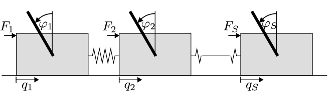
Figure 1: Coupled inverted pendulums on carts.

VI-A Optimal Control Problem Design

We design OCP (1) such that the value function is a Lyapunov function which satisfies inequalities (3). For the sake of reducing the computational burden, our design does not enforce a terminal constraint in the OCP [31]. We choose separable quadratic stage costs $\ell_{i}(x_{i},u_{i})=x_{i}^{\top}Q_{i}x_{i}/2+u_{i}^{\top}R_{i}u_{i}/2,$ where we set $R_{i}=0.001$ and take $Q_{i}=\text{diag}(1,10^{-4},10,10^{-4})$ from [40]. We further design $V_{\text{f},i}(x_{i})={\beta_{2}}x_{i}^{\top}P_{i}x_{i}/2$, where we find $\beta_{2}\geq 1$ and $P_{i}\in\mathbb{R}^{4\times 4}$ as follows. First, we linearize the dynamics $f_{i}^{\delta}$ while neglecting the coupling between carts to obtain a linearized model $(A_{i},B_{i})$ with $A_{i}\in\mathbb{R}^{4\times 4}$ and $B_{i}\in\mathbb{R}^{4\times 1}$ for each subsystem $i$. This allows to solve the algebraic Riccati equation $P_{i}=A_{i}^{\top}P_{i}A_{i}-(A_{i}^{\top}P_{i}B_{i})(R_{i}+B_{i}^{\top}P_{i}B_{i})^{-1}(B_{i}^{\top}P_{i}A_{i})+Q_{i}$ individually for each subsystem to obtain $P_{i}$ and and the terminal control law $u_{i}=K_{i}x_{i}$, where $K_{i}\doteq-(B_{i}^{\top}P_{i}B_{i}+R_{i})^{-1}(B_{i}^{\top}P_{i}A_{i})$. Next, we linearize the dynamics including coupling and obtain the centralized system $(A,B)$ with $A\in\mathbb{R}^{4S\times 4S}$ and $B\in\mathbb{R}^{4S\times S}$. For the example at hand, the terminal controller $K=\text{diag}(K_{1},\dots,K_{S})$ also stabilizes the coupled centralized system, i.e., the matrix $A_{K}=A+BK$ is Schur stable. Denote the centralized weight matrices as $Q\doteq\text{diag}(Q_{1},\dots,Q_{S})$, $R\doteq\text{diag}(R_{1},\dots,R_{S})$, and $P\doteq\text{diag}(P_{1},\dots,P_{S})$. To meet the sufficient decrease condition

$$V_{\text{f}}(f^{\delta}(x,Kx))-V_{\text{f}}(x)\leq-\ell(x,Kx),$$

we increase $\beta_{2}$ until the matrix $\Delta\doteq\tilde{Q}-Q_{K}$ is positive definite, where $\tilde{Q}\doteq\beta_{2}(P-A_{K}^{\top}PA_{k})$ and $Q_{K}\doteq Q+K^{\top}RK$.

Remark 8 (Decentralized $V_{\text{f}}$ design)

The matrices $P_{i}$ and terminal controllers $K_{i}$ are computed by neglecting the coupling of the dynamics and by solving the Riccati equation for each subsystem individually. This simplification is not guaranteed to stabilize coupled linearized systems in general, but the design stabilizes the chain of pendulums considered here. Hence, the matrix $\Delta$ is positive definite for sufficiently large $\beta_{2}$. A similar design approach is suggested in [18, Remark 4]. More elaborate decentralized control designs can be found in the classic textbook [3]. $\square$

VI-B Swing-up Simulation

We consider the swing up of $S=20$ pendulums to analyze the efficacy of the proposed RTI scheme. Our Matlab implementation uses CasADi to evaulate the derivatives in Step 3 of dSQP [41]. The quadratic subproblems in Step 3 of ADMM are solved using OSQP with tolerances $\epsilon_{\text{abs}}=\epsilon_{\text{rel}}=\epsilon_{\text{prim}}=\epsilon_{\text{dual}}=10^{-8}$, where the tolerances are in the notation of [42]. After the control input is computed in each NMPC step, the centralized system is simulated using the explicit Runge-Kutta $4^{\text{th}}$ order method with integration step size $\delta$ to obtain the system state at the next sampling instant. We tune the penalty parameter $\rho$ of ADMM in the set $\{0.1,1,10,100\}$ and choose $\rho=1$.

We compare three test cases with varying initial conditions, OCP designs, and solver settings as summarized in Table I. The pendulums initially rest in the lower equilibrium position $x_{i}(0)=\text{col}(q_{i}(0),0,\pi,0)$, where the initial cart displacement is given in Table I. The goal is to steer all pendulums to the upright equilibrium position at $x_{i}=0$. The OCP is designed with quadratic weights as described in Subsection VI-A. The time horizon is chosen as $T=0.4\,$s and the scaling factors in the objective are set to $\beta=1$ and $\beta_{2}=1.1$. The further parameters in Table I are the shooting interval $h$ in the OCP, the discrete-time horizon $N=T/h$, the chosen Hessian for QP (6), the maximum number of SQP iterations per NMPC step $k_{\text{max}}$, the maximum number of ADMM iterations per SQP iteration $l_{\text{max}}$, the total number of decision variables in the centralized OCP $n$, the total number of subsystem equality constraints $n_{g}$, the total number of subsystem inequality constraints $n_{h}$, and the number of consensus constraints $n_{c}$. For all cases, the control sampling interval is set to $\delta=40\,$ms. For cases one and two, we choose the exact Hessian if $\nabla_{z_{i}z_{i}}^{2}L_{i}$ is positive definite and otherwise we select the GN Hessian. For case three, we always choose the GN Hessian approximation. A quadratic penalty term with weight $10^{-5}$ is added to the objective (1a) for all state copies to meet Assumption 5 (ii). We initialize dSQP in the first NMPC step at a local minimum of the OCP found by ipopt [43]. In all subsequent NMPC steps, we initialize dSQP with the optimizer solution produced in the previous control step.

Table II summarizes the simulation results. We analyze the closed-loop control performance

$$J_{\text{cl}}\doteq\sum_{t=0}^{t_{f}}\sum_{i\in\mathcal{S}}\ell_{i}(x_{i}(t),u_{i}(t)),$$

where $t_{f}$ denotes the number of NMPC steps per simulation, as well as the dSQP execution time per NMPC step on a desktop computer. Specifically, we run each test case ten times to account for varying execution times in between runs and we take two different types of time measurements in each NMPC step. In the first type, we measure the total execution time of one call to dSQP, which is summarized in the second and third columns from the left in Table II. This includes running the specified number of SQP and ADMM iterations for all pendulums in series as well as the costly creation and destruction of intermediate data structures. This is due to the prototypical nature of our Matlab implementation and would be avoided in embedded applications. In the second type of time measurement, summarized in columns four to six of Table II, we measure only imperative code blocks that cannot be avoided in an efficient implementation, and we take measurements for each subsystem individually. This includes calls to CasADi for evaluating derivatives, calls to OSQP for updating and solving QPs in ADMM, and computing Steps 4–5 of ADMM. Column six summarizes the percentage of per-subsystem solve times that were below the sampling interval.

The closed-loop system and optimizer trajectories are shown in Figures 2–3. The top three plots in each Figure display the cart positions, pendulum angles, and control inputs. The optimizer evolutions in the bottom plots show the convergence of dSQP to the OCP solutions $p^{\star}$ found by ipopt.

In all test cases, the pendulums reach the upright equilibrium position while satisfying the input box constraints. Numerical a-posteriori analyses show that the KKT points satisfy Assumption 5 once the system is close to the setpoint, which guarantees local dSQP convergence. The initial cart displacements in the first test case are less challenging than in the second case. In fact, the increase in $k_{\text{max}}$ from the first to the second test case is necessary for a successful swing up due to the different initial conditions. As a result, the computation times increase. While the median per-subsystem computation time in the first test case is smaller than the sampling interval $\delta$, the computation time of the second test case would not be real-time feasible. Therefore, we increase the shooting interval in the third test case to reduce the OCP size and we select the GN Hessian to reduce the time spent evaluating derivatives. As a result, test case three requires less iterations per NMPC step for a successful swing up and the median per-subsystem computation time drops below $\delta$. On the other hand, this reduces performance as can be seen from the prolonged settling time and the increase in $J_{\text{cl}}$. Choosing a shooting interval $h>\delta$ is a well-known technique for reducing RTI computation times [4]. However, the stability guarantees provided by Theorem 2 only hold if $h=\delta$ and if the exact Hessian is chosen. Strictly speaking, the third test case is therefore not covered by the stability guarantees derived in this article.

The time measurements of test cases one and three, obtained for a prototypical Matlab implementation, show that the per-subsystem computation times are mostly below the control sampling interval. This does not imply that an efficient decentralized implementation would necessarily be real-time feasible, in particular if communication latencies add to the computation time. However, the obtained computation times indicate that control sampling intervals in the millisecond range are conceivable via the decentralized RTI scheme.

TABLE I: Test case specifications. All cases consider a sampling interval $\delta=40\,$ms.

Case	$q_{i}(0)$	$h\,$[ms]	$N$	$H$	$k_{\text{max}}$	$l_{\text{max}}$	$n$	$n_{g}$	$n_{h}$	$n_{c}$
1	$-1^{i}$	40	10	exact	1	6	1518	880	400	418
2	$i$	40	10	exact	3	6	1518	880	400	418
3	$i$	80	5	GN	1	4	828	480	240	228

TABLE II: Computation times per NMPC step and closed-loop performance $J_{\text{cl}}$ for a prototypical Matlab implementation. The fast computation times in test cases one and three demonstrate the real-time feasibility of decentralized real-time iterations.

Case	all subsystems combined		per subsystem			$J_{\text{cl}}/10^{4}$
	median [ms]	max. [ms]	median [ms]	max. [ms]	$\leq\delta$
1	332.6	866.4	25.8	76.1	96.84 %	1.4
2	981.1	2828.3	79.2	243.8	00.00 %	3.4
3	196.9	508.4	13.9	56.7	99.99 %	5.2

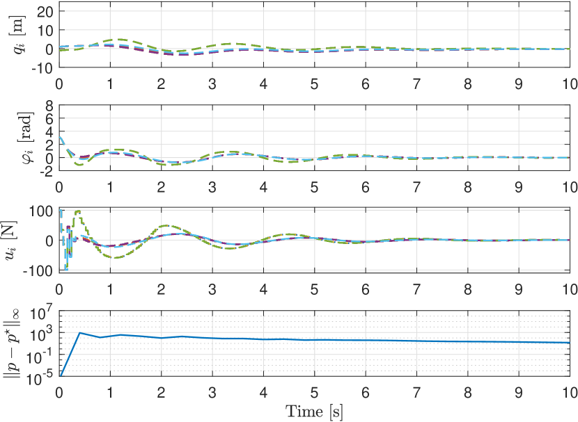
Figure 2: Test case 1: closed-loop system and optimizer convergence with 6 ADMM iterations per NMPC step.

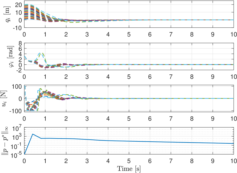
Figure 3: Test case 2: closed-loop system and optimizer convergence for a challenging initial condition with 18 ADMM iterations per NMPC step.

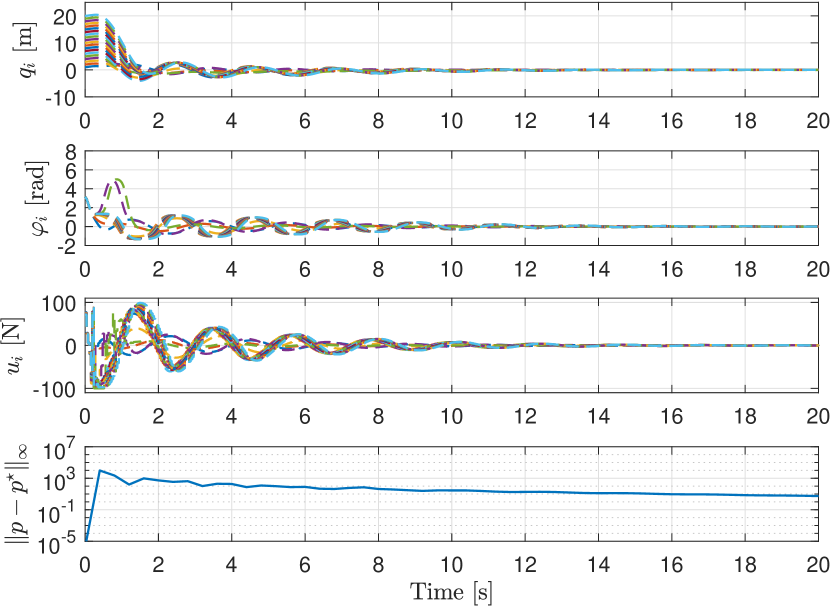
Figure 4: Test case 3: closed-loop system and optimizer convergence with 4 ADMM iterations per NMPC step.

VII Conclusion

This paper has presented a novel decentralized RTI scheme for distributed NMPC based on dSQP. The proposed scheme applies finitely many optimizer iterations per control step and does not require subsystems to exchange information with a coordinator. Stability guarantees are proven for the system-optimizer dynamics in closed loop by combining centralized RTI stability guarantees with novel dSQP convergence results. Numerical simulations demonstrate the efficacy of the proposed scheme for a chain of coupled inverted pendulums. Future work will consider further mechatronic systems and hardware experiments.

References

- [1] A. N. Venkat, I. A. Hiskens, J. B. Rawlings and S. J. Wright “Distributed MPC strategies with application to power system automatic generation control” In IEEE Transactions on Control Systems Technology 16.6, 2008, pp. 1192–1206 DOI: 10.1109/TCST.2008.919414
- [2] Ruben Van Parys and Goele Pipeleers “Distributed MPC for multi-vehicle systems moving in formation” In Robotics and Autonomous Systems 97 Elsevier, 2017, pp. 144–152 DOI: 10.1016/j.robot.2017.08.009
- [3] Dragoslav D Siljak “Decentralized control of complex systems” Academic Press, 1991
- [4] Moritz Diehl, H Georg Bock, Johannes P Schlöder, Rolf Findeisen, Zoltan Nagy and Frank Allgöwer “Real-time optimization and nonlinear model predictive control of processes governed by differential-algebraic equations” In Journal of Process Control 12.4 Elsevier, 2002, pp. 577–585
- [5] Victor M Zavala and Lorenz T Biegler “The advanced-step NMPC controller: Optimality, stability and robustness” In Automatica 45.1 Elsevier, 2009, pp. 86–93
- [6] Inga J Wolf and Wolfgang Marquardt “Fast NMPC schemes for regulatory and economic NMPC–A review” In Journal of Process Control 44 Elsevier, 2016, pp. 162–183
- [7] Andrea Zanelli, Quoc Tran-Dinh and Moritz Diehl “A Lyapunov function for the combined system-optimizer dynamics in inexact model predictive control” In Automatica 134 Elsevier, 2021, pp. 109901
- [8] Bartosz Käpernick and Knut Graichen “The gradient based nonlinear model predictive control software GRAMPC” In 2014 European Control Conference (ECC), 2014, pp. 1170–1175 IEEE
- [9] Moritz Schulze Darup, Gerrit Book and Pontus Giselsson “Towards real-time ADMM for linear MPC” In 2019 18th European Control Conference (ECC), 2019, pp. 4276–4282 IEEE
- [10] Riccardo Scattolini “Architectures for distributed and hierarchical model predictive control – a review” In Journal of Process Control 19.5, 2009, pp. 723–731 DOI: 10.1016/j.jprocont.2009.02.003
- [11] Matthias A. Müller and Frank Allgöwer “Economic and distributed model predictive control: recent developments in optimization-based control” In SICE Journal of Control, Measurement, and System Integration 10.2, 2017, pp. 39–52 DOI: 10.9746/jcmsi.10.39
- [12] Mihajlo D Mesarovic, Donald Macko and Yasuhiko Takahara “Theory of hierarchical, multilevel, systems” Academic Press, New York, 1970
- [13] William B Dunbar “Distributed receding horizon control of dynamically coupled nonlinear systems” In IEEE Transactions on Automatic Control 52.7 IEEE, 2007, pp. 1249–1263
- [14] Matthias A Müller, Marcus Reble and Frank Allgöwer “Cooperative control of dynamically decoupled systems via distributed model predictive control” In International Journal of Robust and Nonlinear Control 22.12 Wiley Online Library, 2012, pp. 1376–1397
- [15] Paolo Varutti, Benjamin Kern and Rolf Findeisen “Dissipativity-based distributed nonlinear predictive control for cascaded systems” In IFAC Proceedings Volumes 45.15 Elsevier, 2012, pp. 439–444
- [16] Christian Conte, Colin N. Jones, Manfred Morari and Melanie N. Zeilinger “Distributed synthesis and stability of cooperative distributed model predictive control for linear systems” In Automatica 69, 2016, pp. 117–125 DOI: 10.1016/j.automatica.2016.02.009
- [17] Anja Bestler and Knut Graichen “Distributed model predictive control for continuous-time nonlinear systems based on suboptimal ADMM” In Optimal Control Applications and Methods 40.1, 2019, pp. 1–23 DOI: 10.1002/oca.2459
- [18] B. T. Stewart, S. J. Wright and J. B. Rawlings “Cooperative distributed model predictive control for nonlinear systems” In Journal of Process Control 21.5 Elsevier, 2011, pp. 698–704 DOI: 10.1016/j.jprocont.2010.11.004
- [19] Tyler H Summers and John Lygeros “Distributed model predictive consensus via the alternating direction method of multipliers” In Proceedings of the 50th Allerton Conference on Communication, Control, and Computing (Allerton), 2012, pp. 79–84
- [20] Jean-Hubert Hours and Colin N. Jones “A parametric nonconvex decomposition algorithm for real-time and distributed NMPC” In IEEE Transactions on Automatic Control 61.2, 2016, pp. 287–302 DOI: 10.1109/TAC.2015.2426231
- [21] Gösta Stomberg, Alexander Engelmann and Timm Faulwasser “A compendium of optimization algorithms for distributed linear-quadratic MPC” In at - Automatisierungstechnik 70.4, 2022, pp. 317–330 DOI: 10.1515/auto-2021-0112
- [22] Dimitri P Bertsekas and John N Tsitsiklis “Parallel and Distributed Computation: Numerical Methods” Englewood Cliffs, NJ: Prentice Hall, 1989
- [23] Angelia Nedić, Alexander Olshevsky and Shi Wei “Decentralized Consensus Optimization and Resource Allocation” In Large-Scale and Distributed Optimization Springer, 2018, pp. 247–287
- [24] Georgios Darivianakis, Annika Eichler and John Lygeros “Distributed model predictive control for linear systems with adaptive terminal sets” In IEEE Transactions on Automatic Control 65.3 IEEE, 2019, pp. 1044–1056
- [25] Johannes Köhler, Matthias A Müller and Frank Allgöwer “Distributed model predictive control—recursive feasibility under inexact dual optimization” In Automatica 102 Elsevier, 2019, pp. 1–9 DOI: 10.1016/j.automatica.2018.12.037
- [26] P. Giselsson and A. Rantzer “On feasibility, stability and performance in distributed model predictive control” In IEEE Transactions on Automatic Control 59.4, 2014, pp. 1031–1036 DOI: 10.1109/TAC.2013.2285779
- [27] Andreas Themelis and Panagiotis Patrinos “Douglas–Rachford splitting and ADMM for nonconvex optimization: Tight convergence results” In SIAM Journal on Optimization 30.1 SIAM, 2020, pp. 149–181
- [28] Yu Wang, Wotao Yin and Jinshan Zeng “Global convergence of ADMM in nonconvex nonsmooth optimization” In Journal of Scientific Computing 78.1, 2019, pp. 29–63 DOI: 10.1007/s10915-018-0757-z
- [29] Gösta Stomberg, Alexander Engelmann and Timm Faulwasser “Decentralized non-convex optimization via bi-level SQP and ADMM” In Proceedings of the 61st IEEE Conference on Decision and Control (CDC), 2022, pp. 273–278 DOI: 10.1109/CDC51059.2022.9992379
- [30] Gösta Stomberg, Henrik Ebel, Timm Faulwasser and Peter Eberhard “Cooperative distributed MPC via decentralized real-time optimization: Implementation results for robot formations” In Control Engineering Practice 138 Elsevier, 2023, pp. 105579
- [31] Daniel Limón, Teodoro Alamo, Francisco Salas and Eduardo F Camacho “On the stability of constrained MPC without terminal constraint” In IEEE Transactions on Automatic Control 51.5 IEEE, 2006, pp. 832–836
- [32] Stephen Boyd, Neal Parikh, Eric Chu, Borja Peleato and Jonathan Eckstein “Distributed optimization and statistical learning via the alternating direction method of multipliers” In Foundations and Trends in Machine Learning 3.1 Hanover, MA, USA: Now Publishers Inc., 2011, pp. 1–122 DOI: 10.1561/2200000016
- [33] Paul T Boggs and Jon W Tolle “Sequential Quadratic Programming” In Acta numerica 4, 1995, pp. 1–51
- [34] Andrea Zanelli “Inexact methods for nonlinear model predictive control: Stability, application, and software”, 2021
- [35] Anthony V Fiacco “Introduction to Sensitivity and Stability Analysis in Nonlinear Programming” Academic Press, 1983
- [36] Wei Hong Yang and Deren Han “Linear Convergence of the Alternating Direction Method of Multipliers for a Class of Convex Optimization Problems” In SIAM Journal on Numerical Analysis 54.2 Society for Industrial and Applied Mathematics, 2016, pp. 625–640 DOI: 10.1137/140974237
- [37] H. G. Bock “Recent advances in parameter identification techniques for ODE” In Numerical Treatment of Inverse Problems in Differential and Integral Equations Boston, MA: Birkhäuser, 1983, pp. 95–121 DOI: 10.1007/978-1-4684-7324-7˙7
- [38] Florian Messerer, Katrin Baumgärtner and Moritz Diehl “Survey of sequential convex programming and generalized Gauss-Newton methods” In ESAIM: Proceedings and Surveys 71 EDP Sciences, pp. 64–88
- [39] Carlo Savorgnan, C Romani, Attila Kozma and Moritz Diehl “Multiple shooting for distributed systems with applications in hydro electricity production” In Journal of Process Control 21.5 Elsevier, 2011, pp. 738–745
- [40] Adam Mills, Adrian Wills and Brett Ninness “Nonlinear model predictive control of an inverted pendulum” In 2009 American Control Conference, 2009, pp. 2335–2340
- [41] Joel A. E. Andersson, Joris Gillis, Greg Horn, James B. Rawlings and Moritz Diehl “CasADi: A Software Framework for Nonlinear Optimization and Optimal Control” In Mathematical Programming Computation 11.1, 2019, pp. 1–36 DOI: 10.1007/s12532-018-0139-4
- [42] Bartolomeo Stellato, Goran Banjac, Paul Goulart, Alberto Bemporad and Stephen Boyd “OSQP: An Operator Splitting Solver for Quadratic Programs” In Mathematical Programming Computation, 2020 DOI: 10.1007/s12532-020-00179-2
- [43] Andreas Wächter and Lorenz T. Biegler “On the Implementation of an Interior-Point Filter Line-Search Algorithm for Large-Scale Nonlinear Programming” In Mathematical Programming 106.1, 2006, pp. 25–57 DOI: 10.1007/s10107-004-0559-y
- [44] R. Findeisen “Nonlinear Model Predictive Control: A Sampled-data Feedback Perspective”, Fortschritt-Berichte VDI: Reihe 8 VDI-Verlag, 2006