Data-dependent density estimation for the Fokker-Planck equation in higher dimensions

Abstract

We present a new strategy to approximate the global solution of the Fokker-Planck equation efficiently in higher dimension and show its convergence. The main ingredients are the Euler scheme to solve the associated stochastic differential equation and a histogram method for tree-structured density estimation on a data-dependent partitioning of the state space $\mathbb{R}^{d}$.

Keywords: Fokker-Planck equation, numerical approximation, tree-structured density estimation, data-dependent partitioning

1 Introduction

Let $d\in\mathbb{N}$, fix $T>0$, and choose a probability density function (pdf, for short) $p_{0}:\mathbb{R}^{d}\to[0,\infty)$ with $\lVert p_{0}\rVert_{\mathbb{L}^{1}}=1$. In this work, we propose and study a new method that uses probabilistic and statistical tools to approximate the global solution $\big{\{}p(t,\cdot)\,;\,t\in[0,T]\big{\}}$ of the Fokker-Planck equation

$$\begin{split}\partial_{t}p(t,\mathbf{x})&=\mathcal{L}^{\ast}p(t,\mathbf{x})\quad\text{for all }\;\,(t,{\bf x})\in(0,T]\times\mathbb{R}^{d},\\ p(0,\mathbf{x})&=p_{0}(\mathbf{x})\quad\text{for all}\;\,\mathbf{x}\in\mathbb{R}^{d}\,,\end{split}$$ (1.1)

in higher dimensions $d$, where

$$\mathcal{L}^{\ast}p(t,\mathbf{x})=-\sum\limits_{i=1}^{d}\partial_{x_{i}}\left(b_{i}(\mathbf{x})\cdot p(t,\mathbf{x})\right)+\frac{1}{2}\sum\limits_{i,j,k=1}^{d}\partial_{x_{i}}\partial_{x_{j}}\left(\sigma_{ik}(\mathbf{x})\cdot\sigma_{jk}(\mathbf{x})\cdot p(t,\mathbf{x})\right)\,$$ (1.2)

is a second-order differential operator, in general, with non-constant coefficients. Under the assumptions stated in Subsection 2.1, there exists a unique classical solution $p:[0,T]\times\mathbb{R}^{d}\to[0,\infty)$ of (1.1) which coincides with the pdf of the related stochastic differential equation (SDE) process $\mathbf{X}\equiv\big{\{}\mathbf{X}_{t}\,;\,t\in[0,T]\big{\}}$, which is given by

$$\begin{split}\mathrm{d}\mathbf{X}_{t}&=\mathbf{b}(\mathbf{X}_{t})\mathrm{d}t+\boldsymbol{\sigma}(\mathbf{X}_{t})\mathrm{d}\mathbf{W}_{t}\qquad\text{for all }t\in(0,T]\\ \mathbf{X}_{0}&=\mathbf{X}^{0}\,;\end{split}$$ (1.3)

see e.g. [22, Prop. 3.3] and [14, Chap. 2, Thm. 1.1]. Here, $\mathbf{b}:\mathbb{R}^{d}\to\mathbb{R}^{d}$ and $\boldsymbol{\sigma}:\mathbf{R}^{d}\to\mathbb{R}^{d\times d}$ are smooth bounded functions with entries $b_{i}(\cdot)$ resp. $\sigma_{ij}(\cdot)$, and $\mathbf{W}\equiv\{\mathbf{W}_{t}\,;\,t\in[0,T]\}$ is a $\mathbb{R}^{d}-$valued Wiener process on a filtered probability space $\bigl{(}\Omega,\mathcal{F},\{\mathcal{F}_{t}\}_{t\geq 0},\mathbb{P}\bigr{)}$, and $\mathbf{X}^{0}$ is random and drawn according to $p_{0}$.

To numerically solve (1.1) in higher dimensions $d\gg 1$, different deterministic and probabilistic methods have been developed in the last two decades and are the subject of active research. For example, well-known deterministic methods to simulate (1.1) in dimensions $d\gg 1$, e.g. include ‘sparse grid’ methods [9], and ‘low-rank approximation’ methods [1, 2], but their efficient use (and theory) is restricted to ‘tensor-sparsity respecting data’ $\mathcal{L}^{\ast}$ and $p_{0}$ in (1.1); see the recent survey in [21, Sec. 2]. A different numerical strategy is to use the probabilistic reformulation (1.3) as a starting point for discretisation and statistical sampling via Monte-Carlo simulations; see e.g. [16]; while the analysis there is exempted from the assumption on ‘tensor-sparsity respecting data’, its straightforward application only yields approximations of values for $p$ from (1.1) at selected space-time points. This work aims at constructing numerical methods for (1.1) and $d\gg 1$ that are based on the probabilistic reinterpretation (1.3) and approximate the ‘entire’ function $p(T,\cdot):\mathbb{R}^{d}\to(0,\infty)$.

From a practical viewpoint, the new Algorithm 1.1 below in this work stands out due to its simple implementability, its intuitive interpretability, and efficiency; from a theoretical viewpoint, its convergence theory covers non-constant $\mathcal{L}^{\ast}\equiv\mathcal{L}^{\ast}(\mathbf{x})$ in higher dimensions $d\gg 1$, which allows broader potential applicability, including the simulation of polymer models, for example, see e.g. [4, 5]. Conceptually, its construction combines

• the (explicit) Euler scheme for (1.3) on a mesh $\{t_{j}\}_{j=0}^{J}\subset[0,T]$ of fixed step size $\tau=\frac{T}{J}$, $J\in\mathbb{N}$, which determines the $\mathbb{R}^{d}-$valued random variable $\mathbf{Y}^{j+1}$ from

  $$\begin{split}\mathbf{Y}^{j+1}&=\mathbf{Y}^{j}+\tau\cdot\mathbf{b}(\mathbf{Y}^{j})+\boldsymbol{\sigma}(\mathbf{Y}^{j})(\mathbf{W}_{t_{j+1}}-\mathbf{W}_{t_{j}})\qquad(j=0,...,J-1)\\ \mathbf{Y}^{0}&=\mathbf{X}^{0}\end{split}$$ (1.4)

  to approximate $\mathbf{X}_{t_{j+1}}$ from (1.3) at time $t_{j+1}=t_{j}+\tau$. The density $p^{J}$ of the induced measure $\mathbb{P}_{\mathbf{Y}^{J}}$ approximates $p(T,\cdot)$ from (1.1); see Theorems 2.1 and 2.2.

• a data-dependent partitioning $\boldsymbol{\mathcal{P}}^{J,\mathtt{M}}$ of $\mathbb{R}^{d}$ based on an $\mathtt{M}$-sample $\mathbf{D}^{J}_{\mathtt{M}}:=\{\mathbf{Y}^{J,m}\}_{m=1}^{\mathtt{M}}$ from (1.4), and statistically equivalent cells [17, Ch. 13] on which the histogram-based estimator $\widehat{\mathtt{p}}^{J,\mathtt{M}}$ for the pdf $p^{J}$ from (1.4) at time $t_{J}=T$ is constructed; see Subsection 3.1.

Such an estimator $\widehat{\mathtt{p}}^{J,\mathtt{M}}$ is advantageous for several reasons:

1. suitability to approximate solutions of (1.1) for $d\gg 1$, where uniform partitioning strategies tend to exhaust even extensive computational resources in the pre-asymptotic range and therefore lose competitivity.

2. automatic construction of adaptive meshes, where locally appearing finer cells $\mathbf{R}_{r}\in\boldsymbol{\mathcal{P}}^{J,\mathtt{M}}$ adjust to local features of the solution $p^{J}:\mathbb{R}^{d}\to[0,\infty)$. The proposed ‘data-dependent’ estimators $\widehat{\mathtt{p}}^{J,\mathtt{M}}:\mathbb{R}^{d}\to[0,\infty)$ below aim to meet two goals at the same time with the help of a single $\mathtt{M}-$sample $\mathbf{D}^{J}_{\mathtt{M}}$: to generate an adaptive mesh $\boldsymbol{\mathcal{P}}^{J,\mathtt{M}}$, and to compute an accurate approximation $\widehat{\mathtt{p}}^{J,\mathtt{M}}$ of $p^{J}$ on that mesh. In approximation theory, generating an underlying partition which depends on the solution itself is referred to as ‘nonlinear approximation’ [11, Section 3.2]; well-known deterministic methods in this direction are ‘adaptive finite elements’ that are applicable in small dimensions $1\leq d\leq 4$, where criteria trigger a repeated automatic local refinement/coarsening of elements with the help of computed local residuals that leads to a final adapted mesh.

In the vein of (b), Algorithm 1.1 below may be seen as a new probabilistic method for the parabolic problem (1.1), which is adaptive in space and whose convergence for general non-constant operators $\mathcal{L}^{\ast}\equiv\mathcal{L}^{\ast}(\mathbf{x})$ follows from Theorem 3.5 in Subsection 3.2. Moreover, the Algorithm 1.1 is applicable in higher dimensions $d\gg 1$ – a property that adaptive finite element methods do not possess.

We now outline the basic steps of our algorithm to solve (1.1) with the help of the tools that were motivated in (a) and (b) above.

Algorithm 1.1.

Let $J\in\mathbb{N}$. Fix an equidistant mesh $\{t_{j}\}_{j=0}^{J}\subset[0,T]$ of mesh-size $\tau=\frac{T}{J}$.

• (Initialization) For $\mathtt{M}\in\mathbb{N}$, generate an i.i.d. $\mathtt{M}-$sample $\mathbf{D}_{\mathtt{M}}^{0}:=\{\mathbf{Y}^{0,m}\}_{m=1}^{\mathtt{M}}$ through sampling via $p_{0}$.

• (Discretization & Sampling) Generate a $\mathtt{M}-$sample $\mathbf{D}_{\mathtt{M}}^{J}:=\{\mathbf{Y}^{J,m}\}_{m=1}^{\mathtt{M}}$ via i.i.d. sample iterates from (1.4).

• (Splitting rule) Use $\mathbf{D}_{\mathtt{M}}^{J}$ to get a data-dependent partitioning $\boldsymbol{\mathcal{P}}^{J,\mathtt{M}}=\{\mathbf{R}_{r};\,r=0,...,\mathtt{R}-1\}$ of $\mathbb{R}^{d}$ into $\mathtt{R}\in\mathbb{N}$ many cells ‘$\mathbf{R}_{r}$’, where each cell contains $k_{\mathtt{M}}\leq\mathtt{M}$ sample iterates.

• (Estimator) Define

  $$\widehat{\mathtt{p}}^{J,\mathtt{M}}(\mathbf{x}):=\sum\limits_{r=0}^{\mathtt{R}-1}\frac{k_{\mathtt{M}}}{\mathtt{M}\cdot\mathtt{vol}(\mathbf{R}_{r})}\cdot\mathbbm{1}_{\{\mathbf{x}\in\mathbf{R}_{r}\}}\,,\qquad\mathbf{x}\in\mathbb{R}^{d}\,,$$ (1.5)

  where $\mathtt{vol}(\mathbf{R}_{r})$ denotes the (possibly infinite) volume of the cell $\mathbf{R}_{r}$.

Two specific splitting rules to generate partitions $\boldsymbol{\mathcal{P}}^{J,\mathtt{M}}$ will be detailed in Section 3: the first rule is due to Gessaman [15] (cf. Gessaman’s rule 3.1), the second one is a modification of the Binary Tree Cuboid (BTC)-splitting rule taken from [13] (cf. BTC-rule 3.3). Both splitting rules generate partitions of statistically equivalent cells, meaning that each cell contains the same number of realisations of $\mathbf{D}_{\mathtt{M}}^{J}$. Our main theoretical result in this work is to prove $\mathbb{P}-a.s.$ convergence of Algorithm 1.1 for Gessaman’s rule 3.1; see Theorem 3.5. More precisely, we prove that for $\widehat{\mathtt{p}}^{J,\mathtt{M}}\equiv\widehat{\mathtt{p}}^{J,\mathtt{M}}_{\mathtt{Ges}}$ in (1.5),

$$\lVert p(T,\cdot)-\widehat{\mathtt{p}}^{J,\mathtt{M}}_{\mathtt{Ges}}\rVert_{\mathbb{L}^{1}}\to 0\qquad\mathbb{P}-a.s.\qquad(\text{for }\mathtt{M}\to\infty\text{ and }\tau\to 0)\,.$$ (1.6)

The following example of non-constant $\mathcal{L}^{\ast}\equiv\mathcal{L}^{\ast}(\mathbf{x})$ in (1.2) illustrates the generation of adaptive meshes in space by Algorithm 1.1.

Example 1.2.

Let $d\in\mathbb{N}$ and $T>0$ initially. Consider (1.1), which corresponds to the associated SDE (1.3) with

$$\mathbf{b}(\mathbf{x})=-\mathbf{x}+\boldsymbol{\beta}\,,\qquad\boldsymbol{\sigma}(\mathbf{x})=\sqrt{2}\cdot\varepsilon\cdot\boldsymbol{Id}_{d}\,,$$

where $\varepsilon>0$, $\boldsymbol{\beta}=[1,...,1]^{\top}\in\mathbb{R}^{d}$, and $\boldsymbol{Id}_{d}$ denotes the $d-$dimensional identity matrix. Let $p_{0}$ be the pdf of the multivariate normal distribution with mean vector $\mathbf{m}_{0}=[0,...,0]^{\top}\in\mathbb{R}^{d}$ and covariance matrix $\mathbf{C}_{0}=\alpha\cdot\boldsymbol{Id}_{d}$, i.e.,

$$p_{0}(\mathbf{x})=\frac{1}{(2\pi\alpha)^{\nicefrac{{d}}{{2}}}}\cdot\exp\left(-\frac{1}{2\alpha}\cdot\lVert\mathbf{x}\rVert_{\mathbb{R}^{d}}^{2}\right)\,,$$ (1.7)

where $\alpha>0$. The true solution of (1.1) is given by (see e.g. [6, Appendix C])

$$p(t,\mathbf{x})=\frac{1}{\sqrt{(2\pi)^{d}\cdot\mathtt{det}(\mathbf{C}_{t})}}\exp\left(-\frac{1}{2}(\mathbf{x}-\mathbf{m}_{t})^{\top}\mathbf{C}_{t}^{-1}(\mathbf{x}-\mathbf{m}_{t})\right)\qquad(t,\mathbf{x})\in[0,T]\times\mathbb{R}^{d}\,,$$ (1.8)

where

$$\mathbf{m}_{t}=[1-\exp(-t),...,1-\exp(-t)]^{\top}\in\mathbb{R}^{d}\,,$$

and

$$\mathbf{C}_{t}=\left(\alpha\cdot\exp(-2t)+\varepsilon^{2}(1-\exp(-2t))\right)\cdot\boldsymbol{Id}_{d}.$$

a) Now fix $d=2$, $T=0.5$, $\tau=\frac{1}{100}$, $\alpha=0.5$, and $\varepsilon=1$. For different choices of $\mathtt{M}$ and $k_{\mathtt{M}}$, Table 1 presents $\mathbb{L}^{\infty}-$errors for the estimator $\widehat{\mathtt{p}}^{J,\mathtt{M}}\equiv\widehat{\mathtt{p}}^{J,\mathtt{M}}_{\mathtt{Ges}}$ given in (1.5) constructed via Algorithm 1.1 with Gessaman’s rule 3.1 in Subsection 3.1.1. For ease of computation, we present errors in the $\mathbb{L}^{\infty}-$norm in all computations; the theoretical convergence results are obtained in the $\mathbb{L}^{1}-$norm.

$\mathtt{M}$	$k_{\mathtt{M}}$	$\lVert p(T,\cdot)-\widehat{\mathtt{p}}_{\mathtt{Ges}}^{J,\mathtt{M}}\rVert_{\mathbb{L}^{\infty}}$	Computational time
$2^{12}$	$2^{6}$	$\approx 0.09$	$3$ sec
$2^{14}$	$2^{7}$	$\approx 0.08$	$11$ sec
$2^{16}$	$2^{8}$	$\approx 0.05$	$43$ sec
$2^{18}$	$2^{9}$	$\approx 0.04$	$172$ sec
$2^{20}$	$2^{10}$	$\approx 0.03$	$698$ sec

Table 1: Example 1.2 a): $\mathbb{L}^{\infty}-$error for $\widehat{\mathtt{p}}^{J,\mathtt{M}}\equiv\widehat{\mathtt{p}}^{J,\mathtt{M}}_{\mathtt{Ges}}$ in (1.5).

b) Now fix $d=2$, $T=1$, $\tau=\frac{1}{100}$, $\alpha=\frac{1}{4\pi}$, and $\varepsilon=\frac{1}{5}$. Figures 1 resp. 2 show snapshots of partitions resp. related solution profiles. We observe automatic migration/adaption of meshes in the direction given by $\boldsymbol{\beta}$.

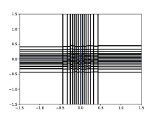
(a) $t=0$, $j=0$

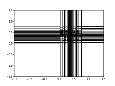
(b) $t=0.5$, $j=50$

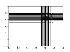
(c) $t=1$, $j=100$

Figure 1: Example 1.2 b): Partition $\boldsymbol{\mathcal{P}}^{j,\mathtt{M}}_{\mathtt{Ges}}$ from Algorithm 1.1 with Gessaman’s rule 3.1; see Subsection 3.1.1 ($\mathtt{M}=2^{16}$, $k_{\mathtt{M}}=2^{8}$).

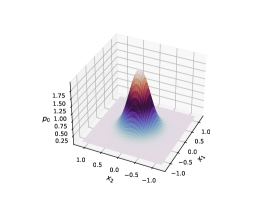
(a) $t=0$, $j=0$

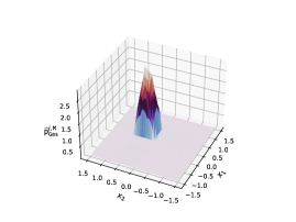
(b) $t=0.5$, $j=50$

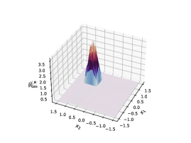
(c) $t=1$, $j=100$

Figure 2: Example 1.2 b): Snapshots for $\widehat{\mathtt{p}}_{\mathtt{Ges}}^{j,\mathtt{M}}$ from Algorithm 1.1 ($\mathtt{M}=2^{16}$, $k_{\mathtt{M}}=2^{8}$).

The estimator $\widehat{\mathtt{p}}^{J,\mathtt{M}}_{\mathtt{Ges}}$ is tree-structured, and each node has exactly $\mathtt{N}=\Big{\lceil}\left(\frac{\mathtt{M}}{k_{\mathtt{M}}}\right)^{\nicefrac{{1}}{{d}}}\Big{\rceil}$ children; see Figure 3 (a). Starting with $\mathcal{R}_{0,0}^{\mathtt{M}}=\mathbb{R}^{d}$ on ‘level $0$’ in the tree in Figure 3 (a), each subsequent node represents a cell in $\mathbb{R}^{d}$, which is recursively split into $\mathtt{N}$ many equiprobable cells until the last (refinement) level $d$ in the tree is reached. After $d$ Gessaman splits, we obtain a tree of height $d$, where the terminal nodes $\{\mathbf{R}_{r}\,;\,r=0,...,\mathtt{R}_{\mathtt{Ges}}-1\}$ with $\mathtt{R}_{\mathtt{Ges}}:=\mathtt{N}^{d}$ constitute the partition $\boldsymbol{\mathcal{P}}_{\mathtt{Ges}}^{J,\mathtt{M}}$; see Figure 3 (a). To increase the limited height of this tree, we also propose the alternative BTC-splitting rule 3.3, which leads to a binary tree of height $\mathcal{O}\left(\log\mathtt{M}\right)$ that enables a much larger degree of local refinement. Here, the terminal nodes $\{\mathbf{R}_{r}\,;\,r=0,...,\mathtt{R}_{\mathtt{BTC}}-1\}$ with $\mathtt{R}_{\mathtt{BTC}}:=2^{\kappa}=\frac{\mathtt{M}}{k_{\mathtt{M}}}$ constitute the partition $\boldsymbol{\mathcal{P}}_{\mathtt{BTC}}^{J,\mathtt{M}}$; see Figure 3 (b). This splitting rule in part 3) of Algorithm 1.1 then builds the density estimator $\widehat{\mathtt{p}}^{J,\mathtt{M}}_{\mathtt{BTC}}$ that is detailed in Subsection 3.1.2.

(a) Generation of partition $\boldsymbol{\mathcal{P}}_{\mathtt{Ges}}^{J,\mathtt{M}}$ with $\mathtt{N}$ splits

(b) Generation of partition $\boldsymbol{\mathcal{P}}_{\mathtt{BTC}}^{J,\mathtt{M}}$ with binary splits

Figure 3: $\mathtt{N}-$ary tree for via Gessaman’s rule 3.1 for $\widehat{\mathtt{p}}^{J,\mathtt{M}}_{\mathtt{Ges}}$ (left) vs. binary tree via BTC-rule 3.3 for $\widehat{\mathtt{p}}^{J,\mathtt{M}}_{\mathtt{BTC}}$ (right).

In this work, we are interested in complex data $\mathbf{D}_{\mathtt{M}}^{J}$ in the sense of [8, p. 8], i.e., data are non-homogeneous and of higher dimension. Here,

• ‘non-homogeneity’ refers to possibly different relationships between the $d$ variables in different parts of $\mathbb{R}^{d}$, which will be triggered by generators $\mathcal{L}^{\ast}\equiv\mathcal{L}^{\ast}(\mathbf{x})$.

• The higher the dimensionality, the sparser and more spread apart the data points are. We approach this difficulty using data-dependent partitions that foremost resolve places in $\mathbb{R}^{d}$ where data points cluster. Our analysis does not assume that the involved variables are independent — as is often supposed for related deterministic schemes to perform efficiently. Our strategy exploits ‘dimensionality reduction’ as suggested in [8, p. 9]; the generated meshing via tree structures fastly segments the data $\mathbf{D}_{\mathtt{M}}^{J}$ into equiprobable cells of the same density, allowing physical interpretation, such as local correlations of the involved $d$ variables.

We continue with an example in $d=5$ where the estimators $\widehat{\mathtt{p}}^{J,\mathtt{M}}_{\mathtt{BTC}}$ and $\widehat{\mathtt{p}}^{J,\mathtt{M}}_{\mathtt{Ges}}$ are compared. We observe an increased accuracy of the former, indicating better adapted meshes.

Example 1.3.

Let $d=5$ and $T=0.3$. Consider (1.1), which corresponds to the associated SDE (1.3) with

$$\mathbf{b}(\mathbf{x})=\mathbf{0}\,,\qquad\boldsymbol{\sigma}(\mathbf{x})=\frac{\sqrt{2}}{8}\cdot\boldsymbol{Id}_{d}\,,$$

where $\mathbf{0}=[0,...,0]^{\top}\in\mathbb{R}^{d}$. Let $p_{0}$ be the pdf from (1.7) with $\alpha>0$. The true solution of (1.1) is given by

$$p(t,\mathbf{x})=\frac{1}{\left(2\pi\alpha+\tfrac{\pi}{16}t\right)^{\nicefrac{{d}}{{2}}}}\cdot\exp\left(-\frac{16}{32\alpha+t}\cdot\lVert\mathbf{x}\rVert_{\mathbb{R}^{d}}^{2}\right)\qquad(t,\mathbf{x})\in[0,T]\times\mathbb{R}^{d}\,.$$

a) For $\tau=\frac{1}{100}$, we consider different choices of $\alpha>0$ in the representation of the initial profile $p_{0}$ in (1.7). The parameter $\alpha$ again quantifies gradients in $p_{0}$. The comparative plots in Figure 4 indicate that $\widehat{\mathtt{p}}^{J,\mathtt{M}}_{\mathtt{BTC}}$ reaches a given accuracy with significantly fewer samples than $\widehat{\mathtt{p}}^{J,\mathtt{M}}_{\mathtt{Ges}}$. As we see in Figure 4 (a), the size $\mathtt{M}$ has to grow when gradients steepen in $p_{0}$ (i.e., $\alpha$ shrinks). Furthermore an initial profile $p_{0}$ with smaller gradients also has a positive impact on the overall performance of Algorithm 1.1: for a fixed choice of $\mathtt{M}=2^{24}$ and $k_{\mathtt{M}}=2^{9}$, the $\mathbb{L}^{\infty}-$error for both $\widehat{\mathtt{p}}^{J,\mathtt{M}}_{\mathtt{Ges}}$ and $\widehat{\mathtt{p}}^{J,\mathtt{M}}_{\mathtt{BTC}}$ is decreasing for increasing $\alpha$; see Figure 4 (b).

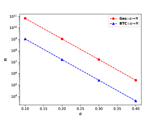
(a) $\alpha\mapsto\mathtt{M}$

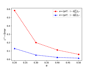
(b) $\alpha\mapsto\lVert p(T,\cdot)-\widehat{\mathtt{p}}^{J,\mathtt{M}}\rVert_{\mathbb{L}^{\infty}}$

Figure 4: Example 1.3 a): (a) Minimum $\mathtt{M}$ for different $\alpha$ to have $\mathbb{L}^{\infty}-$error below $0.1$ (with a fixed ratio of $\mathtt{M}=2^{2N}$ and $k_{\mathtt{M}}=2^{N-2}$, $(N\in\mathbb{N})$). (b) $\mathbb{L}^{\infty}-$error plots for $\widehat{\mathtt{p}}^{J,\mathtt{M}}\equiv\widehat{\mathtt{p}}^{J,\mathtt{M}}_{\mathtt{Ges}}$ resp. $\widehat{\mathtt{p}}^{J,\mathtt{M}}\equiv\widehat{\mathtt{p}}^{J,\mathtt{M}}_{\mathtt{BTC}}$ and different values of $\alpha$ ($\mathtt{M}=2^{24}$, $k_{\mathtt{M}}=2^{9}$).

b) Let $\alpha=\frac{1}{2\pi}$. For $\tau=\frac{1}{100}$, $\mathtt{M}=2^{26}$ and $k_{\mathtt{M}}=2^{11}$, Figure 5 shows the partitions $\boldsymbol{\mathcal{P}}_{\mathtt{Ges}}^{J,\mathtt{M}}$ resp. $\boldsymbol{\mathcal{P}}_{\mathtt{BTC}}^{J,\mathtt{M}}$ of $\mathbb{R}^{5}$ restricted to the plane $\mathbf{P_{1,2}}:=\{(x_{1},x_{2})\,:\,x_{1},x_{2}\in\mathbb{R}\}$. Figure 6 shows the related approximated solutions ${\left.\kern-1.2pt\widehat{\mathtt{p}}^{J,\mathtt{M}}_{\mathtt{Ges}}\mathchoice{\vphantom{\big{|}}}{}{}{}\right|_{\mathbf{P_{1,2}}}}$ resp. ${\left.\kern-1.2pt\widehat{\mathtt{p}}^{J,\mathtt{M}}_{\mathtt{BTC}}\mathchoice{\vphantom{\big{|}}}{}{}{}\right|_{\mathbf{P_{1,2}}}}$, and Figure 7 shows a zoomed view of them from above: while ${\left.\kern-1.2pt\boldsymbol{\mathcal{P}}^{J,\mathtt{M}}_{\mathtt{Ges}}\mathchoice{\vphantom{\big{|}}}{}{}{}\right|_{\mathbf{P_{1,2}}}}$ in Figure 5 (a) looks like a ‘nested tensorised mesh’, the second choice ${\left.\kern-1.2pt\boldsymbol{\mathcal{P}}^{J,\mathtt{M}}_{\mathtt{BTC}}\mathchoice{\vphantom{\big{|}}}{}{}{}\right|_{\mathbf{P_{1,2}}}}$ in Figure 5 (b) detects curved features of the solution; see Figure 7. This increased resolution leads to smaller errors for the estimator $\widehat{\mathtt{p}}^{J,\mathtt{M}}\equiv\widehat{\mathtt{p}}^{J,\mathtt{M}}_{\mathtt{BTC}}$ in Algorithm 1.1; see also Figure 4.

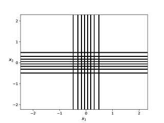
(a) ${\left.\kern-1.2pt\boldsymbol{\mathcal{P}}^{J,\mathtt{M}}_{\mathtt{Ges}}\mathchoice{\vphantom{\big{|}}}{}{}{}\right|_{\mathbf{P_{1,2}}}}$

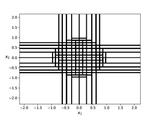
(b) ${\left.\kern-1.2pt\boldsymbol{\mathcal{P}}^{J,\mathtt{M}}_{\mathtt{BTC}}\mathchoice{\vphantom{\big{|}}}{}{}{}\right|_{\mathbf{P_{1,2}}}}$

Figure 5: Example 1.3 b): Partition $\boldsymbol{\mathcal{P}}^{J,\mathtt{M}}_{\mathtt{Ges}}$ resp. $\boldsymbol{\mathcal{P}}^{J,\mathtt{M}}_{\mathtt{BTC}}$ generated via (a) Gessaman’s rule 3.1 resp. (b) BTC-rule 3.3 restricted to $\mathbf{P_{1,2}}$.

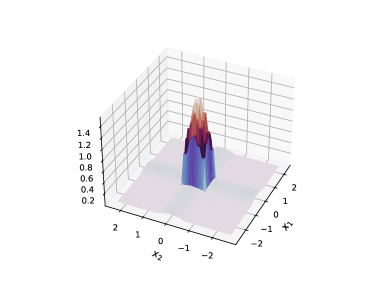
(a) ${\left.\kern-1.2pt\widehat{\mathtt{p}}^{J,\mathtt{M}}_{\mathtt{Ges}}\mathchoice{\vphantom{\big{|}}}{}{}{}\right|_{\mathbf{P_{1,2}}}}$

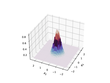
(b) ${\left.\kern-1.2pt\widehat{\mathtt{p}}^{J,\mathtt{M}}_{\mathtt{BTC}}\mathchoice{\vphantom{\big{|}}}{}{}{}\right|_{\mathbf{P_{1,2}}}}$

Figure 6: Example 1.3 b): Approximated solutions (a) $\widehat{\mathtt{p}}^{J,\mathtt{M}}_{\mathtt{Ges}}$ resp. (b) $\widehat{\mathtt{p}}^{J,\mathtt{M}}_{\mathtt{BTC}}$ restricted to $\mathbf{P_{1,2}}$.

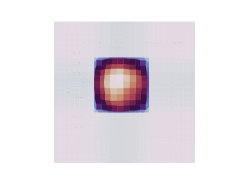
(a) ${\left.\kern-1.2pt\widehat{\mathtt{p}}^{J,\mathtt{M}}_{\mathtt{Ges}}\mathchoice{\vphantom{\big{|}}}{}{}{}\right|_{\mathbf{P_{1,2}}}}$

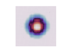
(b) ${\left.\kern-1.2pt\widehat{\mathtt{p}}^{J,\mathtt{M}}_{\mathtt{BTC}}\mathchoice{\vphantom{\big{|}}}{}{}{}\right|_{\mathbf{P_{1,2}}}}$

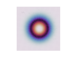
(c) ${\left.\kern-1.2ptp(T,\cdot)\mathchoice{\vphantom{\big{|}}}{}{}{}\right|_{\mathbf{P_{1,2}}}}$

Figure 7: Example 1.3 b): View from above: (a) $\widehat{\mathtt{p}}^{J,\mathtt{M}}_{\mathtt{Ges}}$ resp. (b) $\widehat{\mathtt{p}}^{J,\mathtt{M}}_{\mathtt{BTC}}$ resp. (c) $p(T,\cdot)$ restricted to $\mathbf{P_{1,2}}$.

The next example discusses the performance of the estimator $\widehat{\mathtt{p}}^{J,\mathtt{M}}_{\mathtt{BTC}}$ in a setting when $\mathcal{L}^{\ast}(\mathbf{x})$ given in (1.2) depends on $\mathbf{x}\in\mathbb{R}^{d}$, and where $d=8$.

Example 1.4.

Let $d=8$ and $T=0.2$. Consider (1.1), which corresponds to the associated SDE (1.3) with

$$\mathbf{b}(\mathbf{x})=[0,0,2,2,2,x_{6},x_{7},x_{8}]^{\top}\,,\qquad\boldsymbol{\sigma}(\mathbf{x})=\frac{1+\lVert\mathbf{x}\rVert_{\mathbb{R}^{d}}}{10}\cdot\boldsymbol{Id}_{d}\,.$$

Let $p_{0}$ be the pdf from (1.7) with $\alpha=\frac{1}{2\pi}$. For a fixed choice of $\tau=0.01$, $\mathtt{M}=2^{32}$ and $k_{\mathtt{M}}=2^{10}$, Figure 8 shows approximated solution profiles $\widehat{\mathtt{p}}^{J,\mathtt{M}}_{\mathtt{BTC}}$ when restricted to different coordinate axes. In the style of the notation in Example 1.3, we denote the $x_{i}-$axis by $\mathbf{P_{i}}:=\{x_{i}\,:x_{i}\in\mathbb{R}\}$, $i=1,...,8$. We observe a different structure of $\widehat{\mathtt{p}}^{J,\mathtt{M}}_{\mathtt{BTC}}$ along each coordinate axis mainly due to $\mathbf{b}(\mathbf{x})$, but also $\boldsymbol{\sigma}(\mathbf{x})$: while Figure 8 (a) illustrates the smoothing/flattening dynamics of ${\left.\kern-1.2pt\widehat{\mathtt{p}}^{J,\mathtt{M}}_{\mathtt{BTC}}\mathchoice{\vphantom{\big{|}}}{}{}{}\right|_{\mathbf{P_{1}}}}$ (note that ${\left.\kern-1.2pt\mathbf{b}(\mathbf{x})\mathchoice{\vphantom{\big{|}}}{}{}{}\right|_{\mathbf{P_{1}}}}\equiv 0$ in this case), Figure 8 (b) shows a convection of the approximated solution in the direction given by ${\left.\kern-1.2pt\mathbf{b}(\mathbf{x})\mathchoice{\vphantom{\big{|}}}{}{}{}\right|_{\mathbf{P_{4}}}}\equiv 2$. Figure 8 (c) shows a snapshot of ${\left.\kern-1.2pt\widehat{\mathtt{p}}^{J,\mathtt{M}}_{\mathtt{BTC}}\mathchoice{\vphantom{\big{|}}}{}{}{}\right|_{\mathbf{P_{8,7}}}}$, i.e., of $\widehat{\mathtt{p}}^{J,\mathtt{M}}_{\mathtt{BTC}}$ restricted to the $x_{8}-x_{7}-$plane.

(a) ${\left.\kern-1.2pt\widehat{\mathtt{p}}^{J,\mathtt{M}}_{\mathtt{BTC}}\mathchoice{\vphantom{\big{|}}}{}{}{}\right|_{\mathbf{P_{1}}}}$

(b) ${\left.\kern-1.2pt\widehat{\mathtt{p}}^{J,\mathtt{M}}_{\mathtt{BTC}}\mathchoice{\vphantom{\big{|}}}{}{}{}\right|_{\mathbf{P_{4}}}}$

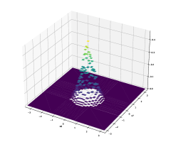
(c) ${\left.\kern-1.2pt\widehat{\mathtt{p}}^{J,\mathtt{M}}_{\mathtt{BTC}}\mathchoice{\vphantom{\big{|}}}{}{}{}\right|_{\mathbf{P_{8,7}}}}$

Figure 8: Example 1.4: Approximated solution profile restricted to different coordinate axes ($\mathtt{M}=2^{32}$, $k_{\mathtt{M}}=2^{10}$).

As mentioned before, our main theoretical result is to verify (1.6) for the density estimator $\widehat{\mathtt{p}}_{\mathtt{Ges}}^{J,\mathtt{M}}$ in Section 3: for this purpose, we first add and subtract the pdf $p^{J}$ of the random variable $\mathbf{Y}^{J}$, and use the triangle inequality to obtain

$$\lVert p(T,\cdot)-\widehat{\mathtt{p}}_{\mathtt{Ges}}^{J,\mathtt{M}}\rVert_{\mathbb{L}^{1}}\leq\underbrace{\lVert p(T,\cdot)-p^{J}\rVert_{\mathbb{L}^{1}}}_{=:{\bf I}}+\underbrace{\lVert p^{J}-\widehat{\mathtt{p}}_{\mathtt{Ges}}^{J,\mathtt{M}}\rVert_{\mathbb{L}^{1}}}_{=:{\bf II}}\qquad\mathbb{P}-a.s.$$ (1.9)

Term ${\bf I}$ in (1.9) measures the error between the pdfs of $\mathbf{X}_{T}$ and $\mathbf{Y}^{J}$, which tends to zero when the time step size $\tau$ tends to zero; for its convergence proof (cf. Theorem 2.2), we benefit from ideas and results in [3]. On the other hand, term ${\bf II}$ measures the error between the pdf $p^{J}$ and its empirical (statistical) counterpart $\widehat{\mathtt{p}}_{\mathtt{Ges}}^{J,\mathtt{M}}$ in (1.5) — which is random — and $\mathbb{P}-a.s.$ converges to zero when $\mathtt{M}$ tends to infinity. The convergence of ${\bf II}$ (cf. Theorem 3.5) builds on the concept of strong $\mathbb{L}^{1}-$consistency of histogram-based density estimators as introduced in [20]. Furthermore we recall from [20] general conditions for a density estimator based on a data-dependent partitioning strategy to be strongly $\mathbb{L}^{1}-$consistent; see Theorem 3.4. The proof of Theorem 3.5 for $\widehat{\mathtt{p}}^{J,\mathtt{M}}\equiv\widehat{\mathtt{p}}^{J,\mathtt{M}}_{\mathtt{Ges}}$ in ${\bf II}$ then consists of verifying the general conditions in Theorem 3.4 for the special estimator $\widehat{\mathtt{p}}^{J,\mathtt{M}}_{\mathtt{Ges}}$ that uses statistically equivalent cells — ensuring that (1.6) holds.

To conclude the introduction, we summarise the advantages of the new method to obtain data-dependent density estimators, which include broad usability to solve (1.1) for non-constant $\mathcal{L}^{\ast}\equiv\mathcal{L}^{\ast}(\mathbf{x})$ in higher dimensions, fast implementation, physical interpretability due to the tree-structured construction (see also [8, p. 55]), mesh adaptivity, and a general convergence theory without strong assumptions on data or solutions. A disadvantage of Algorithm 1.1, however, is the growth of the sample size $\mathtt{M}$ with the dimension $d$ — a problem that we plan to partially compensate in future works by adjusting Algorithm 1.1: Promising tools here include the use of pruning optimal trees [8, Ch. 3] to reduce complexity, and cross-validation [17, Ch.’s 7,8] as well as random forests to stabilise density estimators; moreover, bootstrap methods (‘bagging’; see [7]) may help to generate replicate samplings efficiently. Conceptually, the need for larger $\mathtt{M}-$samples again reflects the ‘curse of dimensionality’, which is inherent to problem (1.1) when we consider general non-structured solutions of (1.1), (1.2), which may only be reduced when additional assumptions are made on data and solutions.
The remainder of this work is organised as follows: Section 2 settles approximability (with rates) of $p(T,\cdot)$ by $p^{J}$. Section 3 shows consistency of the density estimator $\widehat{\mathtt{p}}^{J,\mathtt{M}}_{\mathtt{Ges}}$ from Algorithm 1.1, where Gessaman’s rule 3.1 is used in step 3) of the algorithm; moreover, we introduce the binary-tree-based estimator $\widehat{\mathtt{p}}^{J,\mathtt{M}}_{\mathtt{BTC}}$ with BTC-rule 3.3 as an alternative choice in step 3). Extended computational experiments in Section 4 address practical choices for the parameter $k_{\mathtt{M}}$ to set sample sizes of constructed cells for both density estimators.

2 Assumptions and the law of the Euler scheme

Subsection 2.1 lists basic requirements on data $\mathbf{b}$, $\boldsymbol{\sigma}$ and $p_{0}$ in (1.1) resp. (1.3), which guarantee the existence of the pdfs $p(T,\cdot)$ resp. $p^{J}$ of $\mathbf{X}_{T}$ resp. $\mathbf{Y}^{J}$ from (1.3) resp. (1.4). The results in Subsection 2.2 make sure that $p^{J}$ converges.

2.1 Assumptions on data of the SDE (1.3)

Throughout this work, $\bigl{(}\Omega,\mathcal{F},\{\mathcal{F}_{t}\}_{t\geq 0},\mathbb{P}\bigr{)}$ is a given filtered probability space with natural filtration generated by the Wiener process $\mathbf{W}$ in (1.3). For $1\leq q<\infty$, and a given integrable function $f:\mathbb{R}^{d}\to\mathbb{R}$, we denote by $\lVert f\rVert_{\mathbb{L}^{q}}:=\Big{(}\int\limits_{\mathbb{R}^{d}}\,\lvert f(\mathbf{x})\rvert^{q}\,\mathrm{d}\mathbf{x}\Big{)}^{\nicefrac{{1}}{{q}}}$ the $\mathbb{L}^{q}-$norm of $f$, and by $\lVert f\rVert_{\mathbb{L}^{\infty}}:=\operatorname{ess-sup}\limits_{\mathbf{x}\in\mathbb{R}^{d}}\lvert f(\mathbf{x})\rvert$ the $\mathbb{L}^{\infty}-$norm of $f$. For two sets $\boldsymbol{\mathcal{A}}$ and $\boldsymbol{\mathcal{B}}$, we denote by $\mathcal{C}^{\infty}(\boldsymbol{\mathcal{A}};\boldsymbol{\mathcal{B}})$ the space of all smooth functions $f:\boldsymbol{\mathcal{A}}\to\boldsymbol{\mathcal{B}}$. If $\boldsymbol{\mathcal{B}}=\mathbb{R}$, we write $\mathcal{C}^{\infty}(\boldsymbol{\mathcal{A}})$. Furthermore, we denote by $\mathcal{C}^{\infty}_{0}(\mathbb{R}^{d})$ the space of all smooth functions $f:\mathbb{R}^{d}\to\mathbb{R}$ vanishing at infinity. Moreover, we denote by $\lVert\cdot\rVert_{\mathbb{R}^{d}}$ the Euclidean norm, and by $\langle\cdot,\cdot\rangle_{\mathbb{R}^{d}}$ we denote the corresponding scalar product in $\mathbb{R}^{d}$. In addition, we denote by $\lVert\cdot\rVert_{\mathbb{R}^{d\times d}}$ the spectral matrix norm. Throughout this work, we assume for simplicity:

• $\mathbf{b}\in\mathcal{C}^{\infty}(\mathbb{R}^{d};\mathbb{R}^{d})$, with bounded derivatives of any order.

• $\boldsymbol{\sigma}\in\mathcal{C}^{\infty}(\mathbb{R}^{d};\mathbb{R}^{d\times d})$, with bounded derivatives, and moreover, $\boldsymbol{\sigma}(\cdot)\boldsymbol{\sigma}^{\top}(\cdot)$ satisfies the uniform ellipticity condition, i.e., there exists a constant $\theta>0$, such that

  $$\langle\mathbf{y},\boldsymbol{\sigma}(\mathbf{x})\boldsymbol{\sigma}^{\top}(\mathbf{x})\mathbf{y}\rangle_{\mathbb{R}^{d}}\geq\theta\cdot\lVert\mathbf{y}\rVert_{\mathbb{R}^{d}}^{2}\qquad\text{for all }\mathbf{x},\mathbf{y}\in\mathbb{R}^{d}\,.$$

• $p_{0}:\mathbb{R}^{d}\to[0,\infty)$ is a pdf; in particular $\lVert p_{0}\rVert_{\mathbb{L}^{1}}=1$.

It is well-known that by the assumptions above, there exists a unique classical solution $p:[0,T]\times\mathbb{R}^{d}\to[0,\infty)$ with $p(t,\cdot)\in\mathcal{C}^{\infty}_{0}(\mathbb{R}^{d})$ for all $t\in(0,T]$ of (1.1), which is positive for every fixed time $t\in(0,T]$, i.e., $p(t,\cdot)>0$ on $\mathbb{R}^{d}$; see e.g. [19, Thm. 8.12.1].

2.2 Convergence and properties of the density $p^{J}$ of $\mathbf{Y}^{J}$ from (1.4)

Assumptions (A1) – (A3) in Subsection 2.1 also guarantee the existence of the pdf $p^{J}$ for the random variable $\mathbf{Y}^{J}$ from (1.4); see e.g. [3]. In this subsection, we prove the $\mathbb{P}-a.s.$ convergence of $p^{J}$ to $p(T,\cdot)$ in $\mathbb{L}^{q}$ ($1\leq q\leq\infty$) by extending [3, Corollary 2.7] to include random initial conditions; see Theorem Theorem 2.2 below. First, we introduce some notation: for $\mathbf{y}\in\mathbb{R}^{d}$, we denote by $(t,\mathbf{x})\mapsto p_{\mathbf{y}}(t,\mathbf{x})$ the pdf of the associated SDE process $\mathbf{X}^{\mathbf{y}}\equiv\{\mathbf{X}_{t}^{\mathbf{y}}\,;\,t\in[0,T]\}$, which solves (1.3) with $\mathbf{X}_{0}=\mathbf{y}$. Similarly, we denote by $\mathbf{x}\mapsto p_{\mathbf{y}}^{J}(\mathbf{x})$ the pdf associated with the Euler iterate $\mathbf{Y}^{J}$ from (1.4), where $\mathbf{Y}^{0}=\mathbf{y}\in\mathbb{R}^{d}$. With this notation we have $p(T,\cdot)\equiv p_{\mathbf{X}^{0}}(T,\cdot)$, and $p^{J}(\cdot)\equiv p_{\mathbf{X}^{0}}^{J}(\cdot)$.

Theorem 2.1 ([3, Corollary 2.7]).

Let $J\in\mathbb{N}$, and $\{t_{j}\}_{j=0}^{J}\subset[0,T]$ be a mesh with uniform step size $\tau=\frac{T}{J}$. For all $\mathbf{y},\mathbf{x}\in\mathbb{R}^{d}$ we have

$$\lvert p_{\mathbf{y}}(T,\mathbf{x})-p_{\mathbf{y}}^{J}(\mathbf{x})\rvert\leq C(T)\cdot\tau\cdot\exp\left(-c\frac{\lVert\mathbf{y}-\mathbf{x}\rVert_{\mathbb{R}^{d}}^{2}}{T}\right)\,,$$

where $c>0$, and $C(T)>0$ is a constant that depends on $T$.

For the proof of Theorem 2.1 see [3].

Theorem 2.2.

Let $J\in\mathbb{N}$, and $\{t_{j}\}_{j=0}^{J}\subset[0,T]$ be a mesh with uniform step size $\tau=\frac{T}{J}$. Let $p(T,\cdot)$ and $p^{J}$ be the pdfs of $\mathbf{X}_{T}$ and $\mathbf{Y}^{J}$ from (1.3) resp. (1.4). Then, for $1\leq q\leq\infty$,

$$\lVert p(T,\cdot)-p^{J}\rVert_{\mathbb{L}^{q}}\leq C(T,d,q)\cdot\tau\,,$$

where $C(T,d,q)>0$ is a constant which depends on $T$, $d$, and $q$.

Consequently, for $1\leq q\leq\infty$,

$$\lVert p(T,\cdot)-p^{J}\rVert_{\mathbb{L}^{q}}\to 0\qquad\mathbb{P}-a.s.\qquad(\text{as }\tau\to 0)\,.$$

Proof.

By the Riesz-Thorin interpolation theorem for $\mathbb{L}^{q}$ spaces, it suffices to prove the statement for $q=1$ and $q=\infty$.
Step 1: ($q=1$) By using the Chapman-Kolmogorov equation for the transition density, a calculation yields

$$\lVert p(T,\cdot)-p^{J}\rVert_{\mathbb{L}^{1}} =\int\limits_{\mathbb{R}^{d}}\,\lvert p_{\mathbf{X}^{0}}(T,\mathbf{x})-p_{\mathbf{X}^{0}}^{J}(\mathbf{x})\rvert\,\mathrm{d}\mathbf{x}=\int\limits_{\mathbb{R}^{d}}\,\bigg{\lvert}\int\limits_{\mathbb{R}^{d}}\,p_{\mathbf{y}}(T,\mathbf{x})\cdot p_{0}(\mathbf{y})\,\mathrm{d}\mathbf{y}-\int\limits_{\mathbb{R}^{d}}\,p_{\mathbf{y}}^{J}(\mathbf{x})\cdot p_{0}(\mathbf{y})\,\mathrm{d}\mathbf{y}\,\bigg{\rvert}\,\mathrm{d}\mathbf{x}$$

$$=\int\limits_{\mathbb{R}^{d}}\,\bigg{\lvert}\int\limits_{\mathbb{R}^{d}}\,\left(p_{\mathbf{y}}(T,\mathbf{x})-p_{\mathbf{y}}^{J}(\mathbf{x})\right)\cdot p_{0}(\mathbf{y})\,\mathrm{d}\mathbf{y}\,\bigg{\rvert}\,\mathrm{d}\mathbf{x}\leq\int\limits_{\mathbb{R}^{d}}\,\int\limits_{\mathbb{R}^{d}}\,\big{\lvert}p_{\mathbf{y}}(T,\mathbf{x})-p_{\mathbf{y}}^{J}(\mathbf{x})\big{\rvert}\cdot p_{0}(\mathbf{y})\,\mathrm{d}\mathbf{y}\,\mathrm{d}\mathbf{x}\,.$$

Application of Theorem 2.1 then leads to

$$\lVert p(T,\cdot)-p^{J}\rVert_{\mathbb{L}^{1}} \leq C(T)\cdot\tau\cdot\int\limits_{\mathbb{R}^{d}}\,\int\limits_{\mathbb{R}^{d}}\,\exp\left(-c\frac{\lVert\mathbf{y}-\mathbf{x}\rVert_{\mathbb{R}^{d}}^{2}}{T}\right)\cdot p_{0}(\mathbf{y})\,\mathrm{d}\mathbf{y}\,\mathrm{d}\mathbf{x}$$

$$=C(T)\cdot\tau\cdot\int\limits_{\mathbb{R}^{d}}\,p_{0}(\mathbf{y})\,\int\limits_{\mathbb{R}^{d}}\,\exp\left(-c\frac{\lVert\mathbf{y}-\mathbf{x}\rVert_{\mathbb{R}^{d}}^{2}}{T}\right)\,\mathrm{d}\mathbf{x}\,\mathrm{d}\mathbf{y}\,.$$

Since

$$\int\limits_{\mathbb{R}^{d}}\,\exp\left(-c\frac{\lVert\mathbf{x}-\mathbf{y}\rVert_{\mathbb{R}^{d}}^{2}}{T}\right)\,\mathrm{d}\mathbf{x}=\left(\frac{T\pi}{c}\right)^{\nicefrac{{d}}{{2}}}\,,$$

we further conclude

$$\lVert p(T,\cdot)-p^{J}\rVert_{\mathbb{L}^{1}} \leq C(T)\cdot\tau\cdot\int\limits_{\mathbb{R}^{d}}\,p_{0}(\mathbf{y})\cdot\left(\frac{T\pi}{c}\right)^{\nicefrac{{d}}{{2}}}\,\mathrm{d}\mathbf{y}=C(T)\cdot\left(\frac{T\pi}{c}\right)^{\nicefrac{{d}}{{2}}}\cdot\tau\,,$$

from which the convergence statement in the theorem follows for $q=1$.
Step 2: ($q=\infty$) Similar to Step 1, we obtain

$$\lVert p(T,\cdot)-p^{J}\rVert_{\mathbb{L}^{\infty}} =\sup\limits_{\mathbf{x}\in\mathbb{R}^{d}}\,\lvert p_{\mathbf{X}^{0}}(T,\mathbf{x})-p_{\mathbf{X}^{0}}^{J}(\mathbf{x})\rvert\leq\sup\limits_{\mathbf{x}\in\mathbb{R}^{d}}\,\int\limits_{\mathbb{R}^{d}}\,\big{\lvert}p_{\mathbf{y}}(T,\mathbf{x})-p_{\mathbf{y}}^{J}(\mathbf{x})\big{\rvert}\cdot p_{0}(\mathbf{y})\,\mathrm{d}\mathbf{y}$$

$$\leq C(T)\cdot\tau\cdot\sup\limits_{\mathbf{x}\in\mathbb{R}^{d}}\,\underbrace{\int\limits_{\mathbb{R}^{d}}\,\exp\left(-c\frac{\lVert\mathbf{y}-\mathbf{x}\rVert_{\mathbb{R}^{d}}^{2}}{T}\right)\cdot p_{0}(\mathbf{y})\,\mathrm{d}\mathbf{y}}_{\leq 1}\leq C(T)\cdot\tau\,,$$

from which the convergence assertion follows for $q=\infty$. ∎

3 Data-dependent density estimators

In our opinion, data-dependent partitioning strategies in combination with histogram-based density estimators, which are structured as decision trees, are an intriguing prospect to address the approximation of (1.1); see Figure 3 and Subsection 3.1. In Subsection 3.2, we verify the $\mathbb{P}-a.s.$ $\mathbb{L}^{1}-$convergence of the estimator $\widehat{\mathtt{p}}^{J,\mathtt{M}}\equiv\widehat{\mathtt{p}}^{J,\mathtt{M}}_{\mathtt{Ges}}$ in Algorithm 1.1; see Theorem 3.5.

3.1 On data-dependent partitioning strategies

We present two splitting rules for step 3) in Algorithm 1.1 to obtain two data-dependent estimators $\widehat{\mathtt{p}}^{J,\mathtt{M}}_{\mathtt{Ges}}$ and $\widehat{\mathtt{p}}^{J,\mathtt{M}}_{\mathtt{BTC}}$. For their construction we grow ($\mathtt{N}-$ary resp. binary) trees of different heights, where interior nodes represent an ongoing refinement of the partitioning of $\mathbb{R}^{d}$, which is terminated when the maximum height is reached to explain the structure of the complex data $\mathbf{D}_{\mathtt{M}}^{J}$; see Figure 9.

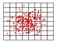
(a) Uniform partition $\boldsymbol{\mathcal{P}}_{\mathtt{uni}}^{J,\mathtt{M}}$

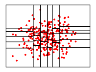
(b) Data-dependent partition $\boldsymbol{\mathcal{P}}_{\mathtt{Ges}}^{J,\mathtt{M}}$

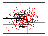
(c) Data-dependent partition $\boldsymbol{\mathcal{P}}_{\mathtt{BTC}}^{J,\mathtt{M}}$

Figure 9: Partitioning of $\mathbb{R}^{d}$, where the sample is drawn from a $2-$dimensional standard normal distribution.

3.1.1 Gessaman’s splitting rule

We fix $\mathtt{M}\in\mathbb{N}$, and let $\mathbf{D}_{\mathtt{M}}^{J}:=\{\mathbf{Y}^{J,m}\}_{m=1}^{\mathtt{M}}$ be an i.i.d. $\mathbb{R}^{d}-$valued sample set from (1.4) with corresponding density $p^{J}$ on $\mathbb{R}^{d}$. Let $k_{\mathtt{M}}\in\mathbb{N}$ denote the number of realizations out of $\mathbf{D}_{\mathtt{M}}^{J}$ of each fully refined cell $\mathbf{R}_{r}\in\boldsymbol{\mathcal{P}}^{J,\mathtt{M}}_{\mathtt{Ges}}$.

For Gessaman’s rule, $\mathbb{R}^{d}$ is partitioned into $\mathtt{N}$ sets using hyperplanes perpendicular to the $x_{1}-$axis, such that each set contains an equal number of samples. This produces $\mathtt{N}$ sets resembling long strips. In the same way, one partitions each of these $\mathtt{N}$ long strips along the $x_{2}-$axis into further $\mathtt{N}$ cells and continues in such a way in all coordinates until $\mathtt{N}^{d}$ cells are reached in total, each containing the same number of sample iterates. More precisely, Gessaman’s rule describes the following algorithm.

Gessaman’s rule 3.1 (see [15, 20]).

Select $\mathtt{M}$ and $k_{\mathtt{M}}$ such that $\mathtt{N}=\Big{\lceil}\left(\frac{\mathtt{M}}{k_{\mathtt{M}}}\right)^{\nicefrac{{1}}{{d}}}\Big{\rceil}\in\mathbb{N}$. Let $\mathcal{R}^{\mathtt{M}}_{0,0}:=\mathbb{R}^{d}$.
For $i=0,...,d$ do:
     For $j=0,...,\mathtt{N}^{i}-1$ do:

• Decompose $\mathcal{R}^{\mathtt{M}}_{i,j}$ into $\mathtt{N}$ hyper-rectangles $\mathcal{R}^{\mathtt{M}}_{i+1,dj+\ell}=\mathcal{R}^{\mathtt{M}}_{i,j}\cap\left(\mathbb{R}^{i}\times[x_{\ell},x_{\ell+1})\times\mathbb{R}^{d-1-i}\right)$ with $x_{\ell}\in\mathbb{R}$ such that $-\infty=x_{0}<x_{1}<...<x_{\mathtt{N}-1}<x_{\mathtt{N}}=\infty$ and each $\mathcal{R}^{\mathtt{M}}_{i+1,dj+\ell}$ contains $\frac{\mathtt{M}}{\mathtt{N}^{i+1}}$ samples. Set $\boldsymbol{\mathcal{P}}_{\mathtt{Ges}}^{J,\mathtt{M}}=\{\mathcal{R}^{\mathtt{M}}_{d,j}\,:\,0\leq j\leq\mathtt{R}_{\mathtt{Ges}}-1\}$, where $\mathtt{R}_{\mathtt{Ges}}=\mathtt{N}^{d}$.

The following example clarifies the construction.

Example 3.2.

Consider Figure 9 (b) in combination with Figure 3 (a). Starting with $\mathcal{R}^{\mathtt{M}}_{0,0}:=\mathbb{R}^{d}$, we observe $\mathtt{N}=6$ long strips in $x_{1}-$direction according to Gessaman’s rule 3.1. For $j=0,..,\mathtt{N}-1$, we denote by $\mathcal{R}^{\mathtt{M}}_{1,j}$ the $j-$th long strip. Then, each of these long strips is further decomposed into $\mathtt{N}=6$ cells. The total amount of cells is $\mathtt{R}_{\mathtt{Ges}}=\mathtt{N}^{2}=36$. For $r=0,...,\mathtt{N}^{2}-1$, we denote by $\mathcal{R}^{\mathtt{M}}_{2,r}\equiv\mathbf{R}_{r}$ the $r-$th cell in the generated partition $\boldsymbol{\mathcal{P}}_{\mathtt{Ges}}^{J,\mathtt{M}}=\{\mathbf{R}_{r};\,r=0,...,\mathtt{R}_{\mathtt{Ges}}-1\}$ with $\mathtt{R}_{\mathtt{Ges}}=\mathtt{N}^{2}$.

3.1.2 A Binary Tree Cuboid (BTC)-based splitting rule

In this subsection, we present an alternative rule leading to trees with a considerably larger depth of $\mathcal{O}(\log(\mathtt{M}))$ and better resolution of the density $p^{J}$. It is a modification of the BTC splitting rule in [13]: In view of condition (c) in Theorem 3.4, longest sides of cells are split recursively to ensure the shrinking of cell diameters. To this end, let $\mathtt{M}=2^{N}$ for some $N\in\mathbb{N}$, and fix a number $k_{\mathtt{M}}=2^{n}$, where $n<N$. The generated partition is denoted by $\boldsymbol{\mathcal{P}}_{\mathtt{BTC}}^{J,\mathtt{M}}$.

BTC-rule 3.3.

Set $\kappa=N-n$, and $\mathcal{S}_{0,0}=\mathbf{D}_{\mathtt{M}}^{J}$, and $\mathcal{R}_{0,0}^{\mathtt{M}}=\mathbb{R}^{d}$.
For $p=0,...,\kappa-1$ do:
     For $q=0,...,2^{p}-1$ do:

• Set $\boldsymbol{\mathcal{S}}:=\mathcal{S}_{p,q}$ and $\boldsymbol{\mathcal{R}}:=\mathcal{R}_{p,q}^{\mathtt{M}}$.

• Find the index of the coordinate axes $\ell\in\{1,...,d\}$ parallel to a largest edge of the cell $\boldsymbol{\mathcal{R}}$; denote this component by $\ell_{p,q}\in\{1,...,d\}$. If two or more edges have equal largest length, choose the edge with the lowest index $\ell$. Edge lengths in a direction in which the cell is unbounded are considered infinite.

• Compute the median $\mathtt{med}_{p,q}\in\mathbb{R}$ along the $\ell_{p,q}-$axis of all sample iterates in $\boldsymbol{\mathcal{S}}$.

• Divide $\boldsymbol{\mathcal{R}}=\mathcal{R}_{p+1,2q}^{\mathtt{M}}\cup\mathcal{R}_{p+1,2q+1}^{\mathtt{M}}$ into two disjoint cells by a hyperplane perpendicular to the $\ell_{p,q}-$axis at $\mathtt{med}_{p,q}$, and set $\mathcal{S}_{p+1,2q}=\boldsymbol{\mathcal{S}}\cap\mathcal{R}_{p+1,2q}^{\mathtt{M}}$, $\mathcal{S}_{p+1,2q+1}=\boldsymbol{\mathcal{S}}\cap\mathcal{R}_{p+1,2q+1}^{\mathtt{M}}$.

Note that ‘$\mathcal{S}_{p,q}$’ contains the samples in ‘$\boldsymbol{\mathcal{S}}$’ which are contained in ‘$\mathcal{R}_{p,q}^{\mathtt{M}}$’. The partition $\boldsymbol{\mathcal{P}}_{\mathtt{BTC}}^{J,\mathtt{M}}$ generated via this procedure has a total number of $\mathtt{R}_{\mathtt{BTC}}:=2^{\kappa}=2^{N-n}=\frac{\mathtt{M}}{k_{\mathtt{M}}}$ cells.

3.2 Strong consistency of the density estimator $\widehat{\mathtt{p}}_{\mathtt{Ges}}^{J,\mathtt{M}}$

The goal of this subsection is to prove the strong $\mathbb{L}^{1}-$consistency of the estimator $\widehat{\mathtt{p}}^{J,\mathtt{M}}_{\mathtt{Ges}}$ from Algorithm 1.1 with Gessaman’s rule 3.1; see Theorem 3.5 below. The combination with Theorem 2.2 then settles convergence of the estimator towards $p(T,\cdot)$ through (1.6).

The density estimator $\widehat{\mathtt{p}}^{J,\mathtt{M}}_{\mathtt{Ges}}$ was first proposed in [15], where its strong $\mathbb{L}^{1}-$consistency was motivated. This section aims to provide a proof of this property. It rests on the verification of three criteria given in [20, Theorem 1] to guarantee strong $\mathbb{L}^{1}-$consistency for a general density estimator; see also Theorem 3.4 below.

Let $\mathtt{M}\in\mathbb{N}$. We write $\boldsymbol{\mathcal{P}}^{J,\mathtt{M}}(\mathbf{x}_{1},...,\mathbf{x}_{\mathtt{M}})$ for a partition of $\mathbb{R}^{d}$ which is realised based upon given points $\mathbf{x}_{1},...,\mathbf{x}_{\mathtt{M}}\in\mathbb{R}^{d}$. Note that with this notation we have $\boldsymbol{\mathcal{P}}^{J,\mathtt{M}}\equiv\boldsymbol{\mathcal{P}}^{J,\mathtt{M}}(\mathbf{Y}^{J,1},...,\mathbf{Y}^{J,\mathtt{M}})$ based on the sample iterates $\mathbf{D}^{J}_{\mathtt{M}}$ from Algorithm 1.1. We denote by $\boldsymbol{\mathcal{A}}_{\mathtt{M}}:=\{\boldsymbol{\mathcal{P}}^{J,\mathtt{M}}(\mathbf{x}_{1},...,\mathbf{x}_{\mathtt{M}})\,:\,\mathbf{x}_{1},...,\mathbf{x}_{\mathtt{M}}\in\mathbb{R}^{d}\}$ the collection of nonrandom partitions following the same underlying partitioning strategy. Moreover, we denote by $\mathtt{m}(\boldsymbol{\mathcal{A}}_{\mathtt{M}}):=\sup\limits_{\boldsymbol{\mathcal{P}}\in\boldsymbol{\mathcal{A}}_{\mathtt{M}}}\#\{\text{cells in }\boldsymbol{\mathcal{P}}\}$ the maximal cell count of $\boldsymbol{\mathcal{A}}_{\mathtt{M}}$.
Fix $\mathtt{M}$ points $\tilde{\mathbf{x}}_{1},...,\tilde{\mathbf{x}}_{\mathtt{M}}\in\mathbb{R}^{d}$ and let $\boldsymbol{\mathcal{B}}:=\{\tilde{\mathbf{x}}_{1},...,\tilde{\mathbf{x}}_{\mathtt{M}}\}$. We denote by $\Delta\bigl{(}\boldsymbol{\mathcal{A}}_{\mathtt{M}},(\tilde{\mathbf{x}}_{1},...,\tilde{\mathbf{x}}_{\mathtt{M}})\bigr{)}$ the number of distinct partitions

$$\{\mathbf{R}_{0}\cap\boldsymbol{\mathcal{B}},...,\mathbf{R}_{\mathtt{R}-1}\cap\boldsymbol{\mathcal{B}}\}$$

of the finite set $\boldsymbol{\mathcal{B}}$ that are induced by partitions $\boldsymbol{\mathcal{P}}:=\{\mathbf{R}_{0},...,\mathbf{R}_{\mathtt{R}-1}\}\in\boldsymbol{\mathcal{A}}_{\mathtt{M}}$. Then, we define the growth function of $\boldsymbol{\mathcal{A}}_{\mathtt{M}}$ as

$$\Delta_{\mathtt{M}}^{\ast}(\boldsymbol{\mathcal{A}}_{\mathtt{M}}):=\max\limits_{(\mathbf{x}_{1},...,\mathbf{x}_{\mathtt{M}})\in\mathbb{R}^{\mathtt{M}\cdot d}}\Delta\bigl{(}\boldsymbol{\mathcal{A}}_{\mathtt{M}},(\mathbf{x}_{1},...,\mathbf{x}_{\mathtt{M}})\bigr{)}\,,$$

which is the largest number of distinct partitions of any $\mathtt{M}$ point subset of $\mathbb{R}^{d}$ that can be induced by the partitions in $\boldsymbol{\mathcal{A}}_{\mathtt{M}}$.
Finally, for every $\mathbf{x}\in\mathbb{R}^{d}$, we denote by $\boldsymbol{\mathcal{P}}^{J,\mathtt{M}}[\mathbf{x}]$ the unique cell in the partition $\boldsymbol{\mathcal{P}}^{J,\mathtt{M}}$ that contains the point $\mathbf{x}$.

Theorem 3.4 ([20, Theorem 1]).

Let $\mathbf{Y}^{J,1},\mathbf{Y}^{J,2},...$ be i.i.d. random vectors in $\mathbb{R}^{d}$ whose common distribution $\mathbb{P}_{\mathbf{Y}^{J}}$ has density $p^{J}$. Let $\mathtt{M}\in\mathbb{N}$. Let $\boldsymbol{\mathcal{A}}_{\mathtt{M}}:=\{\boldsymbol{\mathcal{P}}^{J,\mathtt{M}}(\mathbf{x}_{1},...,\mathbf{x}_{\mathtt{M}})\,:\,\mathbf{x}_{1},...,\mathbf{x}_{\mathtt{M}}\in\mathbb{R}^{d}\}$ be the collection of partitions following the same underlying partitioning strategy. If, as $\mathtt{M}$ tends to infinity

• $\mathtt{M}^{-1}\cdot\mathtt{m}(\boldsymbol{\mathcal{A}}_{\mathtt{M}})\to 0$

• $\mathtt{M}^{-1}\cdot\ln\bigl{(}\Delta_{\mathtt{M}}^{\ast}(\boldsymbol{\mathcal{A}}_{\mathtt{M}})\bigr{)}\to 0$

• $\mathbb{P}_{\mathbf{Y}^{J}}\big{[}\{\mathbf{x}\in\mathbb{R}^{d}\,:\,\mathtt{diam}\bigl{(}\boldsymbol{\mathcal{P}}^{J,\mathtt{M}}[\mathbf{x}]\bigr{)}>\gamma\}\big{]}\to 0\quad\mathbb{P}-a.s.$ for every $\gamma>0$ ,

then the estimator $\widehat{\mathtt{p}}^{J,\mathtt{M}}$ given in (1.5) is strongly $\mathbb{L}^{1}-$consistent, i.e.,

$$\lVert p^{J}-\widehat{\mathtt{p}}^{J,\mathtt{M}}\rVert_{\mathbb{L}^{1}}\to 0\qquad\mathbb{P}-a.s.\qquad\text{(as }\mathtt{M}\to\infty)\,.$$

The next theorem states the strong $\mathbb{L}^{1}-$consistency of the estimator $\widehat{\mathtt{p}}^{J,\mathtt{M}}_{\mathtt{Ges}}$ of Algorithm 1.1, where step 3) is realised via Scheme 3.1.

Theorem 3.5.

Let $J\in\mathbb{N}$, and $\{t_{j}\}_{j=0}^{J}\subset[0,T]$ be a mesh with uniform step size $\tau=\frac{T}{J}$. Let $\mathtt{M}\in\mathbb{N}$ and $k_{\mathtt{M}}\in\mathbb{N}$ with $k_{\mathtt{M}}<\mathtt{M}$. Let $\mathbf{D}_{\mathtt{M}}^{J}:=\{\mathbf{Y}^{J,m}\}_{m=1}^{\mathtt{M}}$ be the sample set from (1.4). If $k_{\mathtt{M}}\to\infty$ and $\frac{k_{\mathtt{M}}}{\mathtt{M}}\to 0$ as $\mathtt{M}\to\infty$, then Gessaman’s estimator $\widehat{\mathtt{p}}^{J,\mathtt{M}}_{\mathtt{Ges}}$ in Algorithm 1.1, where step 3) is realised via Scheme 3.1, is strongly $\mathbb{L}^{1}-$consistent, i.e.,

$$\lVert p^{J}-\widehat{\mathtt{p}}^{J,\mathtt{M}}_{\mathtt{Ges}}\rVert_{\mathbb{L}^{1}}\to 0\qquad\mathbb{P}-a.s.\qquad\text{(as }\mathtt{M}\to\infty)\,.$$

We prove Theorem 3.5 by verifying the conditions (a), (b), and (c) in Theorem 3.4. As we will see, the conditions (a) and (b) automatically follow from the concept of statistically equivalent cells in combination with an appropriate choice of $\mathtt{M}$ and $k_{\mathtt{M}}$. Here, we closely follow the arguments of [20, Theorem 4], which verifies the conditions (a), (b), and (c) of Theorem 3.4 in the case of $d=1$, and therefore proves Theorem 3.5 for $d=1$. The verification of condition (c) for $d\geq 2$, however, is more delicate, and we are not aware of any results in the literature where this part is rigorously proved for Gessaman’s rule 3.1.

Proof of Theorem 3.5..

Let $d\geq 2$.
Verification of (a) in Theorem 3.4: Since we are in the setting of statistically equivalent cells, the number of cells in every partition in $\boldsymbol{\mathcal{A}}_{\mathtt{M}}:=\{\boldsymbol{\mathcal{P}}^{J,\mathtt{M}}_{\mathtt{Ges}}(\mathbf{z}_{1},...,\mathbf{z}_{\mathtt{M}})\,:\,\mathbf{z}_{1},...,\mathbf{z}_{\mathtt{M}}\in\mathbb{R}^{d}\}$ is equal to $\mathtt{R}_{\mathtt{Ges}}:=\mathtt{N}^{d}:=\Big{\lceil}\left(\frac{\mathtt{M}}{k_{\mathtt{M}}}\right)^{\nicefrac{{1}}{{d}}}\Big{\rceil}^{d}$; see Gessaman’s rule 3.1. Hence, due to the growth of $k_{\mathtt{M}}$ related to $\mathtt{M}$, we get

$$\mathtt{M}^{-1}\cdot\mathtt{m}(\boldsymbol{\mathcal{A}}_{\mathtt{M}})=\frac{1}{\mathtt{M}}\cdot\Big{\lceil}\left(\frac{\mathtt{M}}{k_{\mathtt{M}}}\right)^{\nicefrac{{1}}{{d}}}\Big{\rceil}^{d}\to 0\qquad(\text{as }\mathtt{M}\to\infty)\,.$$

Verification of (b) in Theorem 3.4: A combinatorial argument immediately yields (cf. [20, Subsec. 6.3])

$$\Delta_{\mathtt{M}}^{\ast}(\boldsymbol{\mathcal{A}}_{\mathtt{M}})=\binom{\mathtt{M}+\mathtt{R}_{\mathtt{Ges}}}{\mathtt{M}}^{d}\,.$$ (3.1)

We consider the binary entropy function $h(x)=-x\ln(x)-(1-x)\ln(1-x)$, $x\in(0,1)$. We see that $h$ is increasing on $(0,\nicefrac{{1}}{{2}}]$, symmetric about $\nicefrac{{1}}{{2}}$, and $h(x)\to 0$ as $x\to 0$. Using (3.1), the inequality

$$\ln\left(\binom{s}{t}\right)\leq sh\left(\nicefrac{{t}}{{s}}\right)\,,\qquad s,t\in\mathbb{N}$$

stated in [10], and the fact that $h$ is symmetric about $\nicefrac{{1}}{{2}}$, we get

$$\ln\bigl{(}\Delta_{\mathtt{M}}^{\ast}(\boldsymbol{\mathcal{A}}_{\mathtt{M}})\bigr{)} =\ln\left(\binom{\mathtt{M}+\mathtt{R}_{\mathtt{Ges}}}{\mathtt{M}}^{d}\right)=d\cdot\ln\left(\binom{\mathtt{M}+\mathtt{R}_{\mathtt{Ges}}}{\mathtt{M}}\right)\leq d\cdot(\mathtt{M}+\mathtt{R}_{\mathtt{Ges}})\cdot h\left(\frac{\mathtt{M}}{\mathtt{M}+\mathtt{R}_{\mathtt{Ges}}}\right)$$

$$=d\cdot(\mathtt{M}+\mathtt{R}_{\mathtt{Ges}})\cdot h\left(\frac{\mathtt{R}_{\mathtt{Ges}}}{\mathtt{M}+\mathtt{R}_{\mathtt{Ges}}}\right)\,.$$

Since $\mathtt{M}\geq\mathtt{R}_{\mathtt{Ges}}$, $\frac{\mathtt{R}_{\mathtt{Ges}}}{\mathtt{M}+\mathtt{R}_{\mathtt{Ges}}}\leq\frac{1}{k_{\mathtt{M}}}$, we obtain

$$\ln\bigl{(}\Delta_{\mathtt{M}}^{\ast}(\boldsymbol{\mathcal{A}}_{\mathtt{M}})\bigr{)}\leq 2d\cdot\mathtt{M}\cdot h\left(\frac{1}{k_{\mathtt{M}}}\right)\,.$$

Hence, using the properties of $h$ and that $k_{\mathtt{M}}\to\infty$ as $\mathtt{M}\to\infty$, we conclude

$$\mathtt{M}^{-1}\cdot\ln\bigl{(}\Delta_{\mathtt{M}}^{\ast}(\boldsymbol{\mathcal{A}}_{\mathtt{M}})\bigr{)}\leq 2d\cdot h\left(\frac{1}{k_{\mathtt{M}}}\right)\to 0\qquad(\text{as }\mathtt{M}\to\infty)\,.$$

Verification of (c) in Theorem 3.4: Fix $\gamma>0$, $\varepsilon>0$, and let $L\equiv L(\varepsilon)>0$ be such that $\mathbb{P}_{\mathbf{Y}^{J}}[\mathbb{R}^{d}\setminus[-L,L]^{d}]\leq\varepsilon$. Because all cells in the partition $\boldsymbol{\mathcal{P}}^{J,\mathtt{M}}_{\mathtt{Ges}}$ are disjoint excluding the boundary, and due to the choice of $L>0$ above, we find

$$\mathbb{P}_{\mathbf{Y}^{J}}\big{[} \{\mathbf{x}\in\mathbb{R}^{d}\,:\,\mathtt{diam}\bigl{(}\boldsymbol{\mathcal{P}}^{J,\mathtt{M}}_{\mathtt{Ges}}[\mathbf{x}]\bigr{)}>\gamma\}\big{]}\leq\mathbb{P}_{\mathbf{Y}^{J}}\big{[}\{\mathbf{x}\in\mathbb{R}^{d}\,:\,\mathtt{diam}\bigl{(}\boldsymbol{\mathcal{P}}^{J,\mathtt{M}}_{\mathtt{Ges}}[\mathbf{x}]\bigr{)}>\gamma\}\cap[-L,L]^{d}\big{]}+\varepsilon$$

$$=\mathbb{P}_{\mathbf{Y}^{J}}\Bigg{[}\bigcup\limits_{\begin{subarray}{c}r\in\{0,...,\mathtt{R}_{\mathtt{Ges}}-1\}:\\ \mathtt{diam}(\mathbf{R}_{r})\geq\gamma\end{subarray}}\mathbf{R}_{r}\cap[-L,L]^{d}\Bigg{]}+\varepsilon$$

$$=\sum\limits_{r=0}^{\mathtt{R}_{\mathtt{Ges}}-1}\mathbbm{1}_{\{\mathtt{diam}(\mathbf{R}_{r})\geq\gamma\}}\cdot\mathbb{P}_{\mathbf{Y}^{J}}\big{[}\mathbf{R}_{r}\cap[-L,L]^{d}\big{]}+\varepsilon$$

$$\leq\sum\limits_{\begin{subarray}{c}r\in\{0,...,\mathtt{R}_{\mathtt{Ges}}-1\}:\\ \mathbf{R}_{r}\cap[-L,L]^{d}\neq\emptyset\end{subarray}}\mathbbm{1}_{\{\mathtt{diam}(\mathbf{R}_{r})\geq\gamma\}}\cdot\left(\mathbb{P}_{\mathbf{Y}^{J}}[\mathbf{R}_{r}]-\frac{k_{\mathtt{M}}}{\mathtt{M}}+\frac{k_{\mathtt{M}}}{\mathtt{M}}\right)+\varepsilon$$

$$\leq\frac{k_{\mathtt{M}}}{\mathtt{M}}\cdot\sum\limits_{\begin{subarray}{c}r\in\{0,...,\mathtt{R}_{\mathtt{Ges}}-1\}:\\ \mathbf{R}_{r}\cap[-L,L]^{d}\neq\emptyset\end{subarray}}\mathbbm{1}_{\{\mathtt{diam}(\mathbf{R}_{r})\geq\gamma\}}+\sum\limits_{\begin{subarray}{c}r\in\{0,...,\mathtt{R}_{\mathtt{Ges}}-1\}:\\ \mathbf{R}_{r}\cap[-L,L]^{d}\neq\emptyset\end{subarray}}\mathbbm{1}_{\{\mathtt{diam}(\mathbf{R}_{r})\geq\gamma\}}\cdot\Big{\lvert}\mathbb{P}_{\mathbf{Y}^{J}}[\mathbf{R}_{r}]-\frac{k_{\mathtt{M}}}{\mathtt{M}}\Big{\rvert}+\varepsilon\,.$$ (3.2)

Since each cell ‘$\mathbf{R}_{r}$’ is a hyper-rectangle, we can write $\mathbf{R}_{r}=\prod\limits_{i=1}^{d}[a_{i}^{(r)},b_{i}^{(r)}]$ for $a_{i}^{(r)}<b_{i}^{(r)}$. If $\mathtt{diam}(\mathbf{R}_{r}):=\sqrt{\sum\limits_{i=1}^{d}\lvert b_{i}^{(r)}-a_{i}^{(r)}\rvert^{2}}$ is greater or equal to $\gamma$, then its longest side is greater or equal to $\frac{\gamma}{\sqrt{d}}$, i.e., $\max\limits_{i=1,...,d}b_{i}^{(r)}-a_{i}^{(r)}\geq\frac{\gamma}{\sqrt{d}}$. Because the second sum on the right-hand side of (3.2) is bounded from above by

$$\mathbf{E}_{\mathtt{M}}:=\sum\limits_{r=0}^{\mathtt{R}_{\mathtt{Ges}}-1}\Big{\lvert}\mathbb{P}_{\mathbf{Y}^{J}}[\mathbf{R}_{r}]-\frac{k_{\mathtt{M}}}{\mathtt{M}}\Big{\rvert}\,,$$

we therefore conclude from (3.2)

$$\mathbb{P}_{\mathbf{Y}^{J}}\big{[} \{\mathbf{x}\in\mathbb{R}^{d}\,:\,\mathtt{diam}\bigl{(}\boldsymbol{\mathcal{P}}^{J,\mathtt{M}}_{\mathtt{Ges}}[\mathbf{x}]\bigr{)}>\gamma\}\big{]} \leq\frac{k_{\mathtt{M}}}{\mathtt{M}}\cdot\sum\limits_{\begin{subarray}{c}r\in\{0,...,\mathtt{R}_{\mathtt{Ges}}-1\}:\\ \mathbf{R}_{r}\cap[-L,L]^{d}\neq\emptyset\end{subarray}}\mathbbm{1}_{\Big{\{}\max\limits_{i=1,...,d}b_{i}^{(r)}-a_{i}^{(r)}\geq\frac{\gamma}{\sqrt{d}}\Big{\}}}+\mathbf{E}_{\mathtt{M}}+\varepsilon\,.$$ (3.3)

In the following, we estimate the first sum on the right-hand side of (3.3). Standard calculations lead to

$$\sum\limits_{\begin{subarray}{c}r\in\{0,...,\mathtt{R}_{\mathtt{Ges}}-1\}:\\ \mathbf{R}_{r}\cap[-L,L]^{d}\neq\emptyset\end{subarray}} \mathbbm{1}_{\big{\{}\max\limits_{i=1,...,d}b_{i}^{(r)}-a_{i}^{(r)}\geq\tfrac{\gamma}{\sqrt{d}}\big{\}}}$$

$$\leq\sum\limits_{\begin{subarray}{c}r\in\{0,...,\mathtt{R}_{\mathtt{Ges}}-1\}:\\ \mathbf{R}_{r}\subseteq[-L,L]^{d}\end{subarray}}\mathbbm{1}_{\big{\{}\max\limits_{i=1,...,d}b_{i}^{(r)}-a_{i}^{(r)}\geq\tfrac{\gamma}{\sqrt{d}}\big{\}}}+\sum\limits_{\begin{subarray}{c}r\in\{0,...,\mathtt{R}_{\mathtt{Ges}}-1\}:\\ \mathbf{R}_{r}\cap\left(\mathbb{R}^{d}\setminus[-L,L]^{d}\right)\neq\emptyset\end{subarray}}\mathbbm{1}_{\big{\{}\max\limits_{i=1,...,d}b_{i}^{(r)}-a_{i}^{(r)}\geq\tfrac{\gamma}{\sqrt{d}}\big{\}}}$$

$$\leq\#\Big{\{}r=0,...,\mathtt{R}_{\mathtt{Ges}}-1\,:\,\mathbf{R}_{r}\subseteq[-L,L]^{d},\,\max\limits_{i=1,...,d}b_{i}^{(r)}-a_{i}^{(r)}\geq\tfrac{\gamma}{\sqrt{d}}\Big{\}}$$

$$\qquad\qquad+\#\Big{\{}r=0,...,\mathtt{R}_{\mathtt{Ges}}-1\,:\,\mathbf{R}_{r}\cap\left(\mathbb{R}^{d}\setminus[-L,L]^{d}\right)\neq\emptyset\Big{\}}$$

$$\leq\sum\limits_{i=1}^{d}\#\Big{\{}r=0,...,\mathtt{R}_{\mathtt{Ges}}-1\,:\,\mathbf{R}_{r}\subseteq[-L,L]^{d},\,b_{i}^{(r)}-a_{i}^{(r)}\geq\tfrac{\gamma}{\sqrt{d}}\Big{\}}$$

$$\qquad\qquad+\#\Big{\{}r=0,...,\mathtt{R}_{\mathtt{Ges}}-1\,:\,\mathbf{R}_{r}\cap\left(\mathbb{R}^{d}\setminus[-L,L]^{d}\right)\neq\emptyset\Big{\}}\,.$$ (3.4)

Since there are at most $\frac{2L}{\nicefrac{{\gamma}}{{\sqrt{d}}}}$ disjoint intervals of length greater than $\nicefrac{{\gamma}}{{\sqrt{d}}}$ in $[-L,L]$, and the number of cuts along any coordinate axis in Gessaman’s rule 3.1 is at most $\mathtt{N}:=\Big{\lceil}\left(\frac{\mathtt{M}}{k_{\mathtt{M}}}\right)^{\nicefrac{{1}}{{d}}}\Big{\rceil}$, we can bound the first sum in (3.2) by $\sum\limits_{i=1}^{d}\frac{2L}{\nicefrac{{\gamma}}{{\sqrt{d}}}}\cdot\mathtt{N}=d\cdot\sqrt{d}\cdot\frac{2L}{\gamma}\cdot\Big{\lceil}\left(\frac{\mathtt{M}}{k_{\mathtt{M}}}\right)^{\nicefrac{{1}}{{d}}}\Big{\rceil}$ from above. Furthermore, since $[-L,L]^{d}$ has $2d$ sides, we can bound the second summand in (3.2) by $2d\cdot\Big{\lceil}\left(\frac{\mathtt{M}}{k_{\mathtt{M}}}\right)^{\nicefrac{{1}}{{d}}}\Big{\rceil}$ from above. Thus, we conclude

$$\sum\limits_{\begin{subarray}{c}r\in\{0,...,\mathtt{R}_{\mathtt{Ges}}-1\}:\\ \mathbf{R}_{r}\cap[-L,L]^{d}\neq\emptyset\end{subarray}}\mathbbm{1}_{\big{\{}\max\limits_{i=1,...,d}b_{i}^{(r)}-a_{i}^{(r)}\geq\tfrac{\gamma}{\sqrt{d}}\big{\}}}\leq\left(\sqrt{d}\cdot d\cdot\frac{2L}{\gamma}+2d\right)\cdot\Big{\lceil}\left(\frac{\mathtt{M}}{k_{\mathtt{M}}}\right)^{\nicefrac{{1}}{{d}}}\Big{\rceil}\,.$$ (3.5)

Hence, combining (3.5) with (3.3), we get

$$\mathbb{P}_{\mathbf{Y}^{J}}\big{[}\{\mathbf{x}\in\mathbb{R}^{d}\,:\,\mathtt{diam}\bigl{(}\boldsymbol{\mathcal{P}}^{J,\mathtt{M}}_{\mathtt{Ges}}[\mathbf{x}]\bigr{)}>\gamma\}\big{]}\leq\frac{k_{\mathtt{M}}}{\mathtt{M}}\cdot\left(\sqrt{d}\cdot d\cdot\frac{2L}{\gamma}+2d\right)\cdot\Big{\lceil}\left(\frac{\mathtt{M}}{k_{\mathtt{M}}}\right)^{\nicefrac{{1}}{{d}}}\Big{\rceil}+\mathbf{E}_{\mathtt{M}}+\varepsilon\,.$$ (3.6)

Since (a) and (b) in Theorem 3.4 are verified, an application of [20, Corollary 1] yields

$$\mathbf{E}_{\mathtt{M}}\to 0\quad\mathbb{P}-a.s.\quad(\text{ as }\mathtt{M}\to\infty)\,.$$ (3.7)

Finally, by (3.6) and (3.7) we conclude

$$\lim\limits_{\mathtt{M}\to\infty}\mathbb{P}_{\mathbf{Y}^{J}}\big{[}\{\mathbf{x}\in\mathbb{R}^{d}\,:\,\mathtt{diam}\bigl{(}\boldsymbol{\mathcal{P}}^{J,\mathtt{M}}_{\mathtt{Ges}}[\mathbf{x}]\bigr{)}>\gamma\}\big{]}=\varepsilon\quad\mathbb{P}-a.s.\,,$$

which verifies condition (c) of Theorem 3.4.

∎

Remark 3.1.

It is easy to verify parts (a) and (b) in Theorem 3.4 for the BTC-rule 3.3; to verify (c) in this case has to remain open at this stage.

4 Computational experiments

All simulations are conducted via $\mathtt{PYTHON}$ (version 3.11) on a HP ProBook 455 15.6 inch G9 Notebook PC (Processor: AMD Ryzen 7 5825U with Radeon Graphics, 2000 MHz) and on a Dual Xeon 6242 Workstation with 768 GB RAM. In all computational experiments, the samples of the initial conditions are generated with Numpy’s $\mathtt{random.multivariate\_normal}$ command. For the computational evaluation of errors in the $\mathbb{L}^{1}-$norm we use Monte Carlo integration:

$$\lVert f\rVert_{\mathbb{L}^{1}}:=\int\limits_{\mathbb{R}^{d}}\lvert f(\mathbf{x})\rvert\,\mathrm{d}\mathbf{x}\approx\sum\limits_{r=0}^{\mathtt{R}-1}\mathtt{vol}(\mathbf{R}_{r})\cdot\frac{1}{\mathsf{N}}\sum\limits_{n=1}^{\mathsf{N}}\lvert f(\mathbf{x}^{(r)}_{i})\rvert\,,$$

where $\mathsf{N}\in\mathbb{N}$ is sufficiently large, and $\mathbf{x}^{(r)}_{i}$ is a randomly drawn point in the cell $\mathbf{R}_{r}$.
In order to approximate the $\mathbb{L}^{\infty}-$norm, we evaluate the error on each cell $\mathbf{R}_{r}$ at randomly drawn points $\mathbf{x}^{(r)}_{i}\in\mathbf{R}_{r}$ in it, i.e.,

$$\lVert f\rVert_{\mathbb{L}^{\infty}}:=\operatorname{ess-sup}\limits_{\mathbf{x}\in\mathbb{R}^{d}}\lvert f(\mathbf{x})\rvert\approx\max\limits_{r=0,...,\mathtt{R}-1}\max\limits_{i=1,...,\mathsf{N}}\lvert f(\mathbf{x}_{i}^{(r)})\rvert\,,$$

for some $\mathsf{N}\in\mathbb{N}$.

The examples in Section 1 showed the following properties of the density estimator in Algorithm 1.1:
$\bullet$ Example 1.2: for $d=2$ and $\mathcal{L}^{\ast}\equiv\mathcal{L}^{\ast}(\mathbf{x})$, we see an adapted mesh that automatically adjusts to the dynamics of $j\mapsto\widehat{\mathtt{p}}_{\mathtt{Ges}}^{j,\mathtt{M}}$.
$\bullet$ Example 1.3: for $d=5$, the second density estimator $\widehat{\mathtt{p}}_{\mathtt{BTC}}^{J,\mathtt{M}}$ is more efficient, and generates more accurate meshes and results; see also Remark 3.1.
$\bullet$ Example 1.4: we observe corresponding behaviors for $d=8$, and an operator $\mathcal{L}^{\ast}\equiv\mathcal{L}^{\ast}(\mathbf{x})$ with non-constant coefficients.

In the following, we ask about ‘optimal’ choices for $\mathtt{M}$ and $k_{\mathtt{M}}$ in settings where $\varepsilon$ of Example 1.2 decreases, on using Algorithm 1.1 with BTC-rule 3.3.

Continuation of Example 1.2.

Setup	$d$	$T$	$\tau$	$\alpha$	$\varepsilon$
a)	$2$	$1$	$\frac{1}{100}$	$16$	$4$
b)	$2$	$1$	$\frac{1}{100}$	$16$	$\frac{1}{100}$
c)	$2$	$1$	$\frac{1}{100}$	$\frac{1}{20}$	$1$
d)	$2$	$1$	$\frac{1}{100}$	$\frac{1}{20}$	$\frac{1}{100}$

Table 2: Different setups for Example 1.2.

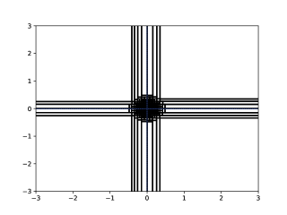
(a) $t=0$

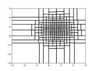
(b) $t=T$

Figure 10: Setup c): Dynamics of the partition $\boldsymbol{\mathcal{P}}_{\mathtt{BTC}}^{J,\mathtt{M}}$ with BTC-rule 3.3 ($\mathtt{M}=2^{16}$, $k_{\mathtt{M}}=2^{8}$).

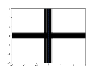
(a) $t=0$

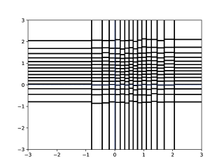
(b) $t=T$

Figure 11: Setup c): Dynamics of the partition $\boldsymbol{\mathcal{P}}_{\mathtt{Ges}}^{J,\mathtt{M}}$ with Gessaman’s rule 3.1 ($\mathtt{M}=2^{16}$, $k_{\mathtt{M}}=2^{8}$).

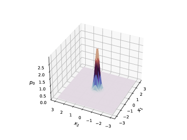
(a) $t=0$

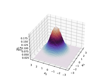
(b) $t=T$

Figure 12: Setup c): Snapshots for $\widehat{\mathtt{p}}_{\mathtt{BTC}}^{J,\mathtt{M}}$ from Algorithm 1.1 ($\mathtt{M}=2^{20}$, $k_{\mathtt{M}}=2^{10}$, $\mathtt{R}=2^{10}$).

Solution (1.8) depends on the choice of $\varepsilon$. In fact, we have for $\mathbf{x}=\mathbf{m}_{t}$, where $p(t,\cdot)$ attains its maximum:

$$\lim\limits_{t\to\infty}p(t,\mathbf{m}_{t})=\frac{1}{(2\pi\varepsilon^{2})^{\nicefrac{{d}}{{2}}}}=\mathcal{O}(\varepsilon^{-d})\,.$$ (4.1)

By comparing the initial profile $p_{0}$ in (1.7) evaluated at $\mathbf{x}=\mathbf{0}$ and (4.1), the simulations show that for

• $\varepsilon>\sqrt{\alpha}$, the profile of the solution (1.8) (as $t\to\infty$) migrates in direction of $\boldsymbol{\beta}$, and its ‘peak value’ flattens to $\frac{1}{(2\pi\varepsilon^{2})^{\nicefrac{{d}}{{2}}}}$, while

• for $\varepsilon<\sqrt{\alpha}$, the profile of the solution (1.8) in fact migrates in direction of $\boldsymbol{\beta}$ too, but its ‘peak value’ grows and sharpens to $\frac{1}{(2\pi\varepsilon^{2})^{\nicefrac{{d}}{{2}}}}$; see Figure 2.

Below, we consider the following challenging scenarios presented in Table 2.

The parameter $\alpha$ also regulates the width and height of $p_{0}$ in (1.7): larger values for $\alpha$ lead to a broader peak of a lower height; whereas small values of $\alpha$ result in a thin and copped peak with a high maximum; see Figure 12 (a). Depending on the relative size of $\varepsilon$ and $\sqrt{\alpha}$, we observe a flattening resp. sharpening of the peak structure up to a certain threshold. This flattening resp. sharpening dynamics comes along with automatic adjustments of the underlying data-dependent partition on which the approximated solution $\widehat{\mathtt{p}}_{\mathtt{BTC}}^{J,\mathtt{M}}$ via Algorithm 1.1 is realised: while flattening dynamics causes an ‘expansion/stretching’ of the partition; see Figures 10 and 11 in the setting of Setup c), sharpening dynamics lead to a ‘concentration/compression’ of the partition; see Figure 1 in Example 1.2.

For a fixed $\mathtt{M}=2^{18}$ and varying $k_{\mathtt{M}}$, Figure 13 below shows $\mathbb{L}^{1}-$ resp. $\mathbb{L}^{\infty}-$errors for $\widehat{\mathtt{p}}_{\mathtt{BTC}}^{J,\mathtt{M}}$ within the scenarios a) – d) in Table 2. While the $\mathbb{L}^{1}-$error curves in Figure 13 (a) are almost the same in every scenario for varying $k_{\mathtt{M}}$, and suggest $k_{\mathtt{M}}\approx\mathtt{M}^{\frac{1}{2}-\beta}$ (for $\beta>0$ small) as optimal choice for smallest $\mathbb{L}^{1}-$errors, the $\mathbb{L}^{\infty}-$error curves in Figure 13 (b) motivate $k_{\mathtt{M}}\approx\mathtt{M}^{\frac{3}{4}\pm\beta}$ (for $\beta>0$ small) for smallest $\mathbb{L}^{\infty}-$errors.

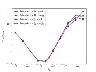
(a) $k_{\mathtt{M}}\mapsto\lVert p(T,\cdot)-\widehat{\mathtt{p}}^{J,\mathtt{M}}_{\mathtt{BTC}}\rVert_{\mathbb{L}^{1}}$

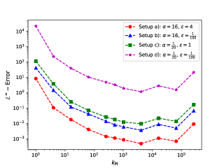
(b) $k_{\mathtt{M}}\mapsto\lVert p(T,\cdot)-\widehat{\mathtt{p}}^{J,\mathtt{M}}_{\mathtt{BTC}}\rVert_{\mathbb{L}^{\infty}}$

Figure 13: Log-plots of $\mathbb{L}^{1}-$ and $\mathbb{L}^{\infty}-$errors with fixed $\mathtt{M}=2^{18}$ and varying $k_{\mathtt{M}}$ within the settings a), b), c) and d).

The next example illustrates the performance of $\widehat{\mathtt{p}}_{\mathtt{BTC}}^{J,\mathtt{M}}$ in Algorithm 1.1 for non-constant $\mathcal{L}^{\ast}\equiv\mathcal{L}^{\ast}(\mathbf{x})$ in (1.2) where the components in $\mathbf{x}\mapsto\mathbf{b}(\mathbf{x})$ and $\mathbf{x}\mapsto\boldsymbol{\sigma}(\mathbf{x})$ are strongly coupled, and where the initial conndition $p_{0}$ is non-continuous.

Example 4.1.

Let $d=8$ and $T=1$. Consider (1.1), which corresponds to the associated SDE (1.3) with

$$\mathbf{b}(\mathbf{x})={\small\begin{bmatrix}0\\ 0\\ 2\\ 2\\ \sin(x_{5})\\ x_{6}\\ x_{8}\\ -x_{7}\\ \end{bmatrix}}\,,\qquad\boldsymbol{\sigma}(\mathbf{x})=0.1\cdot{\small\begin{bmatrix}1&0&0&0&0&0&0&0\\ 0&1&0&0&0&0&0&0\\ 0&0&1&0&0&0&0&0\\ 0&0&0&1&0&0&0&0\\ 0&0&0&0&1&0&0&0\\ 0&0&0&0&0&1&0&0\\ 0&0&0&0&0&0&1&0\\ \arctan(x_{1})^{2}&0&0&0&0&0&0&2+\arctan(x_{1})^{2}\\ \end{bmatrix}}\,,$$

Let $p_{0}$ be the pdf which corresponds to the uniform distribution on the hypercube $[-0.5,0.5]^{d}$. For a fixed choice of $\tau=0.01$, $\mathtt{M}=2^{32}$ and $k_{\mathtt{M}}=2^{10}$, Figure 14 shows approximated solution profiles $\widehat{\mathtt{p}}_{\mathtt{BTC}}^{J,\mathtt{M}}$ when restricted to different coordinate axes, indicating expectable dynamics.

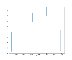
(a) ${\left.\kern-1.2pt\widehat{\mathtt{p}}^{J,\mathtt{M}}_{\mathtt{BTC}}\mathchoice{\vphantom{\big{|}}}{}{}{}\right|_{\mathbf{P_{1}}}}$

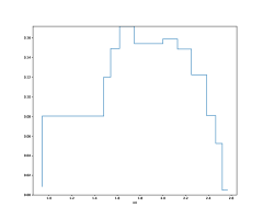
(b) ${\left.\kern-1.2pt\widehat{\mathtt{p}}^{J,\mathtt{M}}_{\mathtt{BTC}}\mathchoice{\vphantom{\big{|}}}{}{}{}\right|_{\mathbf{P_{4}}}}$

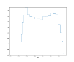
(c) ${\left.\kern-1.2pt\widehat{\mathtt{p}}^{J,\mathtt{M}}_{\mathtt{BTC}}\mathchoice{\vphantom{\big{|}}}{}{}{}\right|_{\mathbf{P_{5}}}}$

Figure 14: Example 4.1: Approximated solution profile restricted to different coordinate axes ($\mathtt{M}=2^{32}$, $k_{\mathtt{M}}=2^{10}$).

Acknowledgement

We are grateful to A. Chaudhary (U Tübingen) for helpful discussions concerning the proof of Theorem 3.5.

References

- [1] M. Bachmayr, R. Schneider, A. Uschmajew, Tensor networks and hierarchical tensors for the solution of high-dimensional partial differential equations, Found. Comput. Math. 16, 1423–1472 (2016).
- [2] M. Bachmayr, Low-rank tensors methods for partial differential equations, Acta Numerica (2023).
- [3] V. Bally, D. Talay, The law of the Euler scheme for stochastic differential equations. II. Convergence rate of the density, Monte Carlo Methods Appl. 2, (1996).
- [4] J.W. Barrett, E. Süli, Existence of global weak solutions to the kinetic Hookean dumbell model in incompressible dilute polymeric fluids, Nonlinear Anal. Real World Appl. 39, pp. 362 – 395 (2018).
- [5] J.W. Barrett, E. Süli, Existence and equilibration of global weak solutions to the kinetic models for dilute polymers II: Hookean-type models, Math. Mod. Meth. Appl. Sci. 22.5 pp. 1150024, 84 (2012).
- [6] N. M. Boffi, E. Vanden Eijnden, Probability flow solution of the Fokker-Planck equation, arXiv preprint, (2023).
- [7] L. Breiman, Bagging predictors, Machine Learning 24, pp. 123-140 (1996).
- [8] L. Breiman, J. Friedman, R. Olsen, C. Stone, Classification and regression trees, Wadsworth (1984).
- [9] H. J. Bungartz, M. Griebel, Sparse grids, Acta Numer. 13, 1–121, (2004).
- [10] I. Csiszár, J. Körner, Information theory: coding theorems for discrete memoryless systems, Academic Press, New York, (1981).
- [11] R.A. De Vore, Nonlinear approximation, Acta Numerica, pp. 51–150 (1998).
- [12] L. Devroye, L. Györfi, and G. Lugosi, A probabilistic theory of pattern recognition, volume 31 of Applications of Mathematics (New York), Springer-Verlag New York (1996).
- [13] T. Dunst, A. Prohl, The forward-backward stochastic heat equation: numerical analysis and simulation, SIAM J. Sci. Comput. 38, (2016).
- [14] M. Freidlin, Functional integration and partial differential equations, Annals of Mathematics Studies 109, Springer, Princeton University Press, Princeton, NJ (1985).
- [15] M. P. Gessaman, A consistent nonparametric multivariate density estimator based on statistically equivalent blocks, Ann. Math. Statist. 41, (1970).
- [16] E. Gobet, Monte-Carlo methods and stochastic processes, CRC Press, Boca Raton (2016).
- [17] L. Györfi, M. Kohler, A. Krzyzak and H. Walk, A distribution-free theory of nonparametric regression, Springer Series in Statistics, Springer-Verlag, New York (2002).
- [18] T. Hastie, R. Tibshirani, and J. Friedman, The elements of statistical learning - data mining, inference, and prediction, Springer (2001).
- [19] N. V. Krylov, Lectures on elliptic and parabolic equations in Hölder spaces, Graduate Studies in Mathematics 12, American Mathematical Society, Providence, RI, (1996).
- [20] G. Lugosi, A. Nobel, Consistency of data-driven histogram methods for density estimation and classification, Ann. Statist. 24, (1996).
- [21] F. Merle, A. Prohl, A posteriori error analysis and adaptivity for high-dimensional elliptic and parabolic boundary value problems, Numer. Math. 153, pp. 827-884 (2023).
- [22] G. A. Pavliotis, Stochastic processes and applications, Texts in Applied Mathematics 60, Springer, New York (2014).