Inference for Cumulative Incidences and Treatment Effects in Randomized Controlled Trials with Time-to-Event Outcomes under ICH E9 (E1)

Abstract

In randomized controlled trials (RCT) with time-to-event outcomes, intercurrent events occur as semi-competing/competing events, and they could affect the hazard of outcomes or render outcomes ill-defined. Although five strategies have been proposed in ICH E9 (R1) addendum to address intercurrent events in RCT, they did not readily extend to the context of time-to-event data for studying causal effects with rigorously stated implications. In this study, we show how to define, estimate, and infer the time-dependent cumulative incidence of outcome events in such contexts for obtaining causal interpretations. Specifically, we derive the mathematical forms of the scientific objective (i.e., causal estimands) under the five strategies and clarify the required data structure to identify these causal estimands. Furthermore, we summarize estimation and inference methods for these causal estimands by adopting methodologies in survival analysis, including analytic formulas for asymptotic analysis and hypothesis testing. We illustrate our methods with the LEADER Trial on investigating the effect of liraglutide on cardiovascular outcomes. Studies of multiple endpoints and combining strategies to address multiple intercurrent events can help practitioners understand treatment effects more comprehensively.

Keywords: Causal inference; Estimand; Intercurrent event; Potential outcome; Randomized controlled trial; Survival analysis.

1 Introduction

Intercurrent events refer to the events “occurring after treatment initiation [of clinical trials] that affect either the interpretation of or the existence of the measurements associated with the clinical question of interest” (International Conference on Harmonization,, 2019). In randomized controlled trials (RCT) with time-to-event outcomes, intercurrent events occur as either semi-competing events which prevent the primary outcome events or competing events which modify the hazard of primary outcome events. Five strategies have been proposed in the International Conference on Harmonization (ICH) E9 (R1) addendum to address intercurrent events, namely, treatment policy strategy, composite variable strategy, while on treatment strategy, hypothetical strategy and principal stratum strategy. These five strategies provide a general guideline for addressing intercurrent events. Different estimands answer different scientific questions. For example, the treatment policy strategy investigates the effect of a “treatment policy”, initial treatment plus the intercurrent events as natural, and the composite variable strategy investigates the treatment effect on a composite outcome, a variable determined jointly by the primary outcome and the intercurrent event.

Several studies have studied the five strategies for binary and continuous outcomes under the potential outcomes framework of causal inference (Lipkovich et al.,, 2020; Ratitch et al.,, 2020; Ionan et al.,, 2023). In particular, a recent study considered the finite sample estimands and elaborated on how to construct these estimands when more than one intercurrent event is anticipated (Han and Zhou,, 2023). However, the insights derived from binary and continuous outcomes do not readily extend to the context of time-to-event outcomes (Young et al., 2020b, ; Siegel et al.,, 2022). When the outcomes are measured at a fixed time point, the potential outcomes under the assigned treatment are observable at the individual level. The causal estimand is a direct contrast of potential outcomes, and it is time-independent. However, due to censoring by loss to follow-up, the potential failure times under the assigned treatments may be unidentifiable when the outcomes are time-to-event, a problem especially relevant to individuals with long potential failure times. As such, the outcome variables of scientific interest often turn to the distribution of potential failure times, such as the cumulative incidence function or survival probability. Therefore, the causal estimands, which reflect the pointwise difference in the distributions of failure times under the treated and control, are time-dependent.

The time-dependent causal estimands bring challenges in estimation and inference. Existing literature in survival analysis has devoted massive efforts to estimating the survival functions when the outcomes are well defined but probably censored (Kaplan and Meier,, 1958; Nelson,, 1972; Aalen,, 1978; Cox,, 1972; Wei,, 1992; Lin et al.,, 1998; Winnett and Sasieni,, 2002). Although it is routine to adjust the events that prevent the outcome measure, the conventional techniques are often ad hoc data analysis-driven, and the resulting estimates may not have causal interpretations. For example, intercurrent events may be viewed as censoring events under the assumption that “censoring” is not informative. This notion is inappropriate because the occurrence of intercurrent events may be related to potential outcomes of interest, leaving the independent “censoring” assumption implausible (Coemans et al.,, 2022).

To account for the competing nature of intercurrent events and primary outcome events, the frameworks of competing risks and semi-competing risks have been proposed. The former views intercurrent events and outcome events as two mutually exclusive events where the occurrence of one event prevents the occurrence of the other (Gray,, 1988; Fine and Gray,, 1999; Andersen et al.,, 2012; Austin et al.,, 2016), while the latter considers one-side exclusion with the occurrence of the primary outcome preventing the intercurrent events only (Fine et al.,, 2001; Huang,, 2021). Some literature reviewed estimands in the presence of competing risks, such as marginal cumulative incidence, cause-specific cumulative incidence (subdistriution function) on the risk scale, as well as marginal hazard, subdistribution hazard, cause-specific hazard on the hazard scale (Gooley et al.,, 1999; Pintilie,, 2007; Lau et al.,, 2009; Geskus,, 2015; Emura et al.,, 2020; Young et al., 2020b, ). In general, estimands on the risk scale lead to better causal interpretation than those on the hazard scale because timewise hazards are comparing individuals with different underlying features (Martinussen and Vansteelandt,, 2013; Aalen et al.,, 2015). Estimation methods to derive estimates were proposed under the frameworks of competing risks and semi-competing risks, including copula modelling, frailty modelling, maximum likelihood estimation, influence function theory and Bayesian inference (Xu et al.,, 2010; Comment et al.,, 2019; Gao et al.,, 2022; Martinussen and Stensrud,, 2021; Xu et al.,, 2022; Nevo and Gorfine,, 2022).

However, these works were more motivated by specific problems in analysis with (semi-)competing risks, rather than providing a comprehensive understanding of the five strategies proposed by ICH E9 (R1) with time-to-event outcomes. Indeed, the medical community is calling for a comprehensive and rigorous approach to following the ICH E9 (R1) in the context of time-to-event data (Kahan et al.,, 2020; Cro et al.,, 2022). It is important to guide clinical practitioners to define, estimate, infer, and interpret the estimands under the strategies from a causal perspective. In this paper, we study the case where there is a time-to-event primary outcome and a possible time-to-event intercurrent event. We describe the time-dependent causal estimands under the five strategies in ICH E9 (R1) for time-to-event outcomes. We provide nonparametric estimation, inference and hypothesis testing methods in RCT with independent censoring by adopting methodologies in survival analysis. Finally, we illustrate these five strategies using a real-world clinical trial, the LEADER (Liraglutide Effect and Action in Diabetes: Evaluation of cardiovascular outcome Results) Trial (Marso et al.,, 2016). The proposed estimation methods are easily implementable, and are applicable to studying various scientific questions of interest. The insights of our proposed framework can be easily extended to accommodate multiple types of intercurrent events by combining strategies for each intercurrent events. Studies of multiple endpoints and combining strategies to address multiple intercurrent events can help practitioners understand treatment effects more comprehensively.

The remainder of this paper is organized as follows. In §2, we define estimands under the strategies in ICH E9 (R1). In §3, we provide nonparametric Nelson-Aalen estimators and asymptotic variances to construct pointwise confidence intervals. In §4, we derive hypothesis testing methods based on log-rank tests. We summarize a comparison between these five strategies in §5, and apply these methods to the LEADER Trial in §6. Finally, we conclude this study with a brief discussion in §7.

2 Estimands for time-to-event outcomes

In this section, we describe the time-dependent causal estimands under the five strategies to address intercurrent events. We shall adopt the potential outcomes framework (Rubin,, 1974) that defines a causal estimand as the contrast between functionals of potential outcomes.

Consider a randomized controlled trial with $n$ individuals randomly assigned to one of the two treatment conditions denoted by $w$, with $w=1$ representing the active treatment (a test drug) and $w=0$ the control (placebo). An upper limit for the study duration of interest since the treatment initiation is set to be $t^{*}$. Assume all patients adhere to treatment assignments and there is no treatment discontinuation before $t^{*}$. For illustration, assume there is at most one intercurrent event. As such, associated with individual $i=1,\ldots,n$ are two potential time-to-event primary outcomes $T_{i}(1)$ and $T_{i}(0)$, if any, which represent the time durations from treatment initiation to the primary outcome event under two treatment assignments respectively. Let $R_{i}(1)$ and $R_{i}(0)$ denote the occurrence time of potential intercurrent events, if any, under the two treatment assignments respectively. If primary outcome events are prevented by intercurrent events under treatment condition $w$, we denote $T_{i}(w)=\infty$. Intercurrent events are considered as absent if no post-treatment intercurrent events occur until $t^{*}$, in which case we denote $R_{i}(w)=\infty$ or an arbitrary number larger than $t^{*}$, since only the events before $t^{*}$ will be counted in analysis.

We shall introduce estimands without the notations of censoring because censoring refers to the problem of missing data and should not affect the definition of estimands. Censoring will be considered in §3 when discussing identification and estimation methods. We adopt the counterfactual cumulative incidences under both treatment assignments as the target estimands, that is, the timewise probability that the primary outcome event will occur by appropriately adjusting intercurrent events. Cumulative incidences are collapsible and enjoy causal interpretations. We focus on the treatment effect defined as the difference in counterfactual cumulative incidences because it has the most straightforward form. Other forms of treatment effects like restricted mean time lost can also be derived, by contrasting the integrated cumulative incidences (Zhao et al.,, 2016; Conner and Trinquart,, 2021).

We will hereby suppress the individual $i$ subscript, because the random vector for each individual is assumed to be drawn independently from a distribution common to all individuals. In the following, we use $\mathsf{Pr}(\cdot)$ to denote the probability taken with randomized sampling and treatment assignment, $\mathsf{E}(\cdot)$ the expectation, and $\mathsf{I}(\cdot)$ the indicator function. We let $\mu_{1}^{k}(t)$ and $\mu_{0}^{k}(t)$, $k\in\{\text{tp, cv, hp, wo, ps}\}$ , $0\leq t\leq t^{*}$, denote the cumulative incidences of two potential outcomes of interest under the treatment policy strategy, composite variable strategy, hypothetical strategy, while on treatment strategy and principal stratum strategy, respectively. The mathematical forms of $\mu_{1}^{k}(t)$ and $\mu_{0}^{k}(t)$ will be illustrated below.

Treatment policy strategy

The treatment policy strategy addresses the problem of intercurrent events by expanding the initial treatment conditions to a treatment policy. This strategy is valid only if primary outcome events cannot be prevented by intercurrent events. Treatments under comparison are now two treatment policies, the assignment of test drug plus the occurrence of intercurrents as natural versus the assignment of placebo plus the occurrence of intercurrents as natural. Instead of comparing the test drug and placebo themselves, the contrast of interest is made between the two treatment policies. The difference in cumulative incidences under the two treatment policies is then

$$\tau^{\text{tp}}(t) :=\mu_{1}^{\text{tp}}(t)-\mu_{0}^{\text{tp}}(t)$$ (1)

$$:=\mathsf{Pr}(T(1,R(1))<t)-\mathsf{Pr}(T(0,R(0))<t),$$

representing the difference in probabilities of experiencing primary outcome events during $[0,t)$ under active treatment and placebo.

The average treatment effect $\tau^{\text{tp}}(t)$ has a meaningful causal interpretation only when $T(1,R(1))$ and $T(0,R(0))$ are well defined. Because the treatment policy includes the occurrence of the intercurrent event as natural, we can simplify the notations $T(w,R(w))=T(w)$ in defining estimands, $w=1,0$. As such, $\tau^{\text{tp}}(t)=\mathsf{Pr}(T(1))<t)-\mathsf{Pr}(T(0)<t)$ as the intention-to-treat analysis.

Composite variable strategy

The composite variable strategy addresses the problem of intercurrent events by expanding the outcome variables. It aggregates the intercurrent events and primary outcome variable as one composite outcome variable. The idea is not new in the notion of progression-free survival (Broglio and Berry,, 2009; Fleming et al.,, 2009), where the composite outcome variable may be defined as the occurrence of either the non-terminal event (e.g., cancer progression) or terminal event (e.g., death). One widely used composite outcome variable has the form $R(w)\wedge T(w)=\min\{T(w),R(w)\}$ for $w\in\{1,0\}$. When this simple form is adopted, the difference in counterfactual cumulative incidences is

$$\tau^{\text{cv}}(t) :=\mu_{1}^{\text{cv}}(t)-\mu_{0}^{\text{cv}}(t)$$ (2)

$$:=\mathsf{Pr}(R(1)\wedge T(1)<t)-\mathsf{Pr}(R(0)\wedge T(0)<t),$$

representing the difference in probabilities of experiencing either intercurrent events or primary outcome events during $[0,t)$ under active treatment and placebo. Other composite forms of $T(w)$ and $R(w)$ are also available, e.g., the composite variable as quality-adjusted lifetime which imposes different weights for the pre- and post-intercurrent periods (Goldhirsch et al.,, 1989; Cole et al.,, 1996; Revicki et al.,, 2006).

While on treatment strategy

The while on treatment strategy considers the measure of outcome variables taken only up to the occurrence of intercurrent events. The failures of primary outcome events should not be counted in the cumulative incidences $\mu_{w}^{\text{wo}}(t)$, $w=1,0$, if intercurrent events occurred. The difference in counterfactual cumulative incidences under this strategy is

$$\tau^{\text{wo}}(t) :=\mu_{1}^{\text{wo}}(t)-\mu_{0}^{\text{wo}}(t)$$ (3)

$$:=\mathsf{Pr}(T(1)<t,R(1)\geq t)-\mathsf{Pr}(T(0)<t,R(0)\geq t),$$

representing the difference in probabilities of experiencing primary outcome events without intercurrent events during $[0,t)$ under active treatment and placebo. The $\mu_{w}^{\text{wo}}(t)$ is also known as cause-specific cumulative incidence or subdistribution function (Geskus,, 2011; Lambert et al.,, 2017).

The while on treatment strategy is closely related to the competing risks models widely used in medical studies (Fine and Gray,, 1999; Lau et al.,, 2009; Andersen et al.,, 2012). However, for causal interpretations, it is worth emphasizing that the hazard of $R(1)$ may differ from that of $R(0)$, leading to vast difference in the underlying features of individuals who have not experienced primary outcome events between treatment conditions until any time $0\leq t\leq t^{*}$. Therefore, if the scientific question of interest is the impact of treatment on the primary outcomes, the estimand $\tau^{\text{wo}}(t)$ is hard to interpret if systematic difference in the risks of intercurrent events between the treatment conditions under comparison are anticipated (Latouche et al.,, 2013; Han and Zhou,, 2023). Under the multi-state model framework, let the original status, intercurrent events status and primary outcome events status be three compartments, then $\mu_{w}^{\text{wo}}(t)$ is the probability of being in the state of primary outcome events, whereas $\mu_{w}^{\text{cv}}(t)$ is the probability of being in either state of intercurrent events or primary outcome events under treatment condition $w$ (Bühler et al.,, 2023).

Hypothetical strategy

The hypothetical strategy envisions a hypothetical clinical trial condition where the occurrence of intercurrent events is restricted in certain ways. By doing so, the distribution of potential outcomes under the hypothetical scenario can capture the impact of intercurrent events explicitly through a pre-specified criterion. We use $T^{\prime}(w)$, $w=1,0$ to denote the time to the primary outcome event in the hypothetical scenario. The time-dependent treatment effect specific to this hypothetical scenario is written as

$$\tau^{\text{hp}}(t) :=\mu_{1}^{\text{hp}}(t)-\mu_{0}^{\text{hp}}(t)$$ (4)

$$:=\mathsf{Pr}(T^{\prime}(1)<t)-\mathsf{Pr}(T^{\prime}(0)<t),$$

representing the difference in probabilities of experiencing primary outcome events during $[0,t)$ in the pre-specified hypothetical scenario under active treatment and placebo.

There can be many hypothetical scenarios envisioned by manipulating the hazard specific to intercurrent events

$$d\Lambda_{2}(t;w)=\mathsf{Pr}(t\leq R(w)<t+dt\mid T(w)\geq t,R(w)\geq t),$$

while assuming the hazard specific to primary outcome events

$$d\Lambda_{1}(t;w)=\mathsf{Pr}(t\leq T(w)<t+dt\mid T(w)\geq t,R(w)\geq t)$$

is left unchanged, where $w=1,0$ and $0\leq t\leq t^{*}$. Let $d\Lambda_{2}^{\prime}(t;w)$ and $d\Lambda_{1}^{\prime}(t;w)$ be the hazards specific to intercurrent events and primary outcome events in the hypothetical scenario respectively, with $d\Lambda_{1}^{\prime}(t;w)=d\Lambda_{1}(t;w)$, $w=1,0$. For example, we can envision a scenario where the intercurrent events when individuals were assigned to test drugs were only permitted if such intercurrent events would have occurred if these individuals were assigned to placebo. In this hypothetical scenario, when assigned to placebo, individuals would be equally likely to experience intercurrent events as they are assigned to placebo in the real-world trial in terms of the hazards; when assigned to test drug, the hazard of intercurrent events would be identical to that if assigned to placebo in the real-world trial. That is, $d\Lambda_{2}^{\prime}(t;0)=d\Lambda_{2}^{\prime}(t;1)=d\Lambda_{2}(t;0)$. We call this the hypothetical scenario I, and denote the corresponding estimand as $\tau^{\text{hp,I}}(t)$. Alternatively, we can envision another hypothetical scenario where the intercurrent events are absent in the hypothetical scenario for all individuals (Robins and Greenland,, 1992; Young et al., 2020a, ). We call this hypothetical scenario II, and denote the corresponding estimand as $\tau^{\text{hp,II}}(t)$. In this scenario, $d\Lambda_{2}^{\prime}(t;0)=d\Lambda_{2}^{\prime}(t;1)=0$. This hypothetical scenario II leads to an estimand called the marginal cumulative incidence.

The hypothetical strategy is closely related with mediation analysis which is intended to evaluate the direct and indirect effects (Lange and Hansen,, 2011; Martinussen et al.,, 2011; Tchetgen Tchetgen,, 2011). The invariance of the hazard specific to primary outcome events when manipulating the hazard specific to intercurrent events is referred to as sequential ignorability in mediation analysis, and is also called dismissible treatment components in separable effects approach (Martinussen and Stensrud,, 2021, 2023). Other hypothetical scenarios can be envisioned for semi-competing risks data by controlling the prevalence or hazard of intercurrent events (Huang,, 2021; Deng et al.,, 2023; Breum et al.,, 2024).

Principal stratum strategy

The principal stratum strategy aims to stratify the population into subpopulations based on the joint potential occurrences of intercurrent events under the two treatment assignments $(R(1),R(0))$ (Frangakis and Rubin,, 2002; Gao et al.,, 2022; Bornkamp et al.,, 2021). Suppose we are interested in a principal stratum comprised of individuals who would never experience intercurrent events regardless of receiving which treatment. This principal stratum can be indicated by $\{R(1)=R(0)=\infty\}$. The treatment effect is now defined within this subpopulation,

$$\tau^{\text{ps}}(t) :=\mu_{1}^{\text{ps}}(t)-\mu_{0}^{\text{ps}}(t)$$ (5)

$$:=\mathsf{Pr}(T(1)<t\mid R(1)=R(0)=\infty)$$

$$\qquad-\mathsf{Pr}(T(0)<t\mid R(1)=R(0)=\infty),$$

representing the difference in probabilities of experiencing primary outcome events during $[0,t]$ under active treatment and placebo in the subpopulation who will not experience intercurrent events regardless of treatments during $[0,t]$.

However, the target population is impossible to identify, not only because values of $R(1)$ and $R(0)$ are never observed simultaneously, but also due to the problem of censoring so that whether $R(w)$ equals $\infty$ is unknown even under the assigned treatment condition $w$. The interpretation of the terget population should be paid special attention, because the composition of the target population relies on the choice of $t^{*}$ (Comment et al.,, 2019). The target population would get smaller with increasing $t^{*}$ except if there is an upper limit, which is smaller than $t^{*}$ alomst surely, for the occurrence time of intercurrent events. Typically, untestable assumptions are attended to identify the principal stratum estimand. Sensitivity analysis is recommended along with principal stratum strategy to assess the robustness of conclusions to untestable assumptions (Gilbert et al.,, 2003; Stuart and Jo,, 2015; Wang et al.,, 2023).

3 Identification and estimation

3.1 Data structure and notations with censoring

Before describing the observed data structure, we update our notations to account for censoring. Each individual is then associated with two potential right censoring times $C(1)$ and $C(0)$. Because of censoring, we are able to only partially observe potential primary outcome events through $\Delta^{T}(w)=\mathsf{I}\{T(w)\leq C(w)\}$ and $\tilde{T}(w)=\min\{T(w),C(w)\}$, and potential intercurrent events through $\Delta^{R}(w)=\mathsf{I}\{R(w)\leq C(w)\}$ and $\tilde{R}(w)=\min\{R(w),C(w)\}$. We assume the stable unit treatment value assumption (SUTVA), which ensures that the individuals are independent and there are only two potential outcomes for each event corresponding to each treatment condition (Rubin,, 1980). We also assume causal consistency, so the observed variables are equal to those potential variables under the actual assignment $W$, that is, $\tilde{T}=\tilde{T}(W)$, $\Delta^{T}=\Delta^{T}(W)$, $\tilde{R}=\tilde{R}(W)$, and $\Delta^{R}=\Delta^{R}(W)$.

The observed data structure can be simplified according to how intercurrent events compete with primary outcome events. If the intercurrent events do not prevent the occurrence of the primary outcome events, our observed data has a structure of $(W,\tilde{T},\tilde{R},\Delta^{T},\Delta^{R})$. On the other hand, if the intercurrent events can prevent the occurrence of the primary outcome events, our observed data structure has the form $(W,\tilde{T}\wedge\tilde{R},\Delta^{T},\Delta^{R})$. The latter structure involves less information and can be derived from the former.

To identify the causal estimands described in §2, we list the following four assumptions.

Assumption 1 (Randomization).

$W\perp(T(1),T(0),R(1),R(0))$.

Assumption 2 (Independent censoring).

$C(w)\perp(T(w),R(w))\mid W=w$, for $w=1,0$.

Assumption 3 (Positivity).

$\mathsf{Pr}(T(w)>t^{*},R(w)>t^{*},C^{*}(w)>t^{*},W=w)>0$, for $w=1,0$.

Assumption 4 (Principal ignorability).

$T(w)\perp R(1-w)\mid R(w)$, for $w=1,0$.

Assumptions 1–3 should be made under all these five strategies for the purpose of identification, and Assumption 4 is added under the principal stratum strategy. Although the principal stratum estimand can be identified under other assumptions instead of Assumption 4, we adopt Assumption 4 because it is the most common and easy-to-interpret assumption in principal sratification methodologies (Ding and Lu,, 2017).

Below, we shall focus on the hazard function of potential outcomes to identify causal estimands, because the independent censoring assumption ensures missingness at random given at-risk sets at each time point.

3.2 Treatment policy strategy

3.2.1 Identification

Under Assumptions 1–3, the hazard function of the potential primary outcome event can be identified through

$$d\Lambda(t;w) :=\mathsf{Pr}(t\leq T(w)<t+dt\mid T(w)\geq t)$$

$$=\mathsf{Pr}(t\leq\tilde{T}(w)<t+dt,\Delta^{T}(w)=1\mid\tilde{T}(w)\geq t),$$

$$=\mathsf{Pr}(t\leq\tilde{T}<t+dt,\Delta^{T}=1\mid\tilde{T}\geq t,W=w),\quad w=1,0.$$

Because $\mu_{w}^{\text{tp}}(t)=\mathsf{Pr}(T(w,R(w))<t)=\mathsf{Pr}(T(w)<t)=1-\exp\{-\Lambda(t;w)\}$, we can identify $\tau^{\text{tp}}(t)$ as

$$\tau^{\text{tp}}(t) =\exp\{-\Lambda(t;0)\}-\exp\{-\Lambda(t;1)\}.$$

3.2.2 Estimation

To estimate this quantity, we use the data on the primary outcome events in the presence of censoring, $(\tilde{T},\Delta^{T},W)$. We write the event process and at-risk process of the primary outcome event as follows,

$$N(t;w) =\sum_{i=1}^{n}\mathsf{I}\{\tilde{T}_{i}\leq t,\Delta^{T}_{i}=1,W_{i}=w\},$$

$$Y(t;w) =\sum_{i=1}^{n}\mathsf{I}\{\tilde{T}_{i}\geq t,W_{i}=w\},\quad w=1,0.$$

The cumulative hazard function $\Lambda(t;w)$, $w=1,0$ is then consistently and unbiasedly estimated by the Nelson-Aalen estimator

$$\widehat{\Lambda}(t;w)=\int_{0}^{t}\frac{dN(s;w)}{Y(s;w)}.$$

We shall estimate $\mu_{w}^{\text{tp}}(t)$ and $\tau^{\text{tp}}(t)$ by the plug-in estimator using the estimated hazards $\widehat{\Lambda}(t;w)$, denoted by $\widehat{\mu}_{w}^{\text{tp}}(t)$ and $\widehat{\tau}^{\text{tp}}(t)$ respectively. The pointwise asymptotic variances of $\widehat{\mu}_{w}^{\text{tp}}(t)$ and $\widehat{\tau}^{\text{tp}}(t)$ are

$$\mathrm{avar}\{\widehat{\mu}_{w}^{\text{tp}}(t)\} =\exp\{-2\Lambda(t;w)\}\cdot\int_{0}^{t}\frac{d\Lambda(s;w)}{\mathsf{Pr}(\tilde{T}\geq s,W=w)},$$

$$\mathrm{avar}\{\widehat{\tau}^{\text{tp}}(t)\} =\mathrm{avar}\{\widehat{\mu}_{1}^{\text{tp}}(t)\}+\mathrm{avar}\{\widehat{\mu}_{0}^{\text{tp}}(t)\},$$

which can be consistently estimated by plug-in estimators. Thus, the confidence intervals of $\mu_{w}^{\text{tp}}(t)$ and $\tau^{\text{tp}}(t)$ can be constructed based on the normal approximation.

3.3 Composite variable strategy

3.3.1 Identification

Under Assumptions 1–3, the hazard function of the composite outcome variable, the potential minimum event time $T(w)\wedge R(w)$, can be identified through

$$d\Lambda_{12}(t;w) :=\mathsf{Pr}(t\leq T(w)\wedge R(w)<t+dt\mid T(w)\wedge R(w)\geq t)$$

$$=\mathsf{Pr}(t\leq\tilde{T}\wedge\tilde{R}<t+dt,\Delta^{T}\vee\Delta^{R}=1\mid\tilde{T}\wedge\tilde{R}\geq t,W=w).$$

Under the treatment condition $w$, the probability that an individual experiences a composite outcome event before $t$ is $\mu_{w}^{\text{cv}}(t)=1-\exp\{-\Lambda_{12}(t;w)\}$. The estimand $\tau^{\text{cv}}(t)$ is identified as

$$\tau^{\text{cv}}(t)=\exp\{-\Lambda_{12}(t;0)\}-\exp\{-\Lambda_{12}(t;1)\}.$$

3.3.2 Estimation

To estimate this quantity, we collect data on the earlier one of the primary outcome event and intercurrent event. The data have the structure of $(\tilde{T}\wedge\tilde{R},\Delta^{T}\vee\Delta^{R},W)$. Identically, we shall focus on the estimation of hazards, and then estimate $\mu_{w}^{\text{cv}}(t)$ and $\tau^{\text{cv}}(t)$ by the plug-in estimators.

We write the event process and at-risk process of the composite outcome event as follows,

$$N_{12}(t;w) =\sum_{i=1}^{n}\mathsf{I}\{\tilde{T}_{i}\wedge\tilde{R}_{i}\leq t,\Delta^{T}_{i}\vee\Delta^{R}_{i}=1,W_{i}=w\},$$

$$Y_{12}(t;w) =\sum_{i=1}^{n}\mathsf{I}\{\tilde{T}_{i}\wedge\tilde{R}_{i}\geq t,W_{i}=w\}.$$

The cumulative hazard function $\Lambda_{12}(t;w)$, $w=1,0$ is consistently and unbiasedly estimated by

$$\widehat{\Lambda}_{12}(t;w)=\int_{0}^{t}\frac{dN_{12}(s;w)}{Y_{12}(s;w)}.$$

The pointwise asymptotic variances of the plug-in estimators of $\mu_{w}^{\text{cv}}(t)$ and $\tau^{\text{cv}}(t)$ are given by

$$\mathrm{avar}\{\widehat{\mu}_{w}^{\text{cv}}(t)\} =\exp\{-2\Lambda_{12}(t;w)\}\cdot\int_{0}^{t}\frac{d\Lambda_{12}(s;w)}{\mathsf{Pr}(\tilde{T}\wedge\tilde{R}\geq s,W=w)},$$

$$\mathrm{avar}\{\widehat{\tau}^{\text{cv}}(t)\} =\mathrm{avar}\{\widehat{\mu}_{1}^{\text{cv}}(t)\}+\mathrm{avar}\{\widehat{\mu}_{0}^{\text{cv}}(t)\}.$$

3.4 While on treatment strategy

3.4.1 Identification

We denote the hazard specific to the primary outcome event and the hazard specific to the intercurrent event by

$$d\Lambda_{1}(t;w) =\mathsf{Pr}(t\leq T(w)<t+dt\mid T(w)\geq t,R(w)\geq t),$$

$$d\Lambda_{2}(t;w) =\mathsf{Pr}(t\leq R(w)<t+dt\mid T(w)\geq t,R(w)\geq t),$$

respectively, where $w=1,0$. Under Assumptions 1–3, they are identified as

$$d\Lambda_{1}(t;w) =\mathsf{Pr}(t\leq\tilde{T}<t+dt,\Delta^{T}=1\mid\tilde{T}\geq t,\tilde{R}\geq t,W=w),$$

$$d\Lambda_{2}(t;w) =\mathsf{Pr}(t\leq\tilde{R}<t+dt,\Delta^{R}=1\mid\tilde{T}\geq t,\tilde{R}\geq t,W=w).$$

The sum of these two hazards, $d\Lambda_{1}(t;w)+d\Lambda_{2}(t;w)$, is the hazard of developing either primary outcome event or intercurrent event, which is exactly the same as the hazard under the composite variable outcome, that is,

$$d\Lambda_{1}(t;w)+d\Lambda_{2}(t;w)=d\Lambda_{12}(t;w).$$

Because $\mu_{w}^{\text{wo}}(t)=\mathsf{Pr}(T(w)<t,R(w)\geq t)=\int_{0}^{t}\exp\{-\Lambda_{12}(s;w)\}d\Lambda_{1}(s;w)$, $w=1,0$, the estimand $\tau^{\text{wo}}(t)$ is identified as

$$\tau^{\text{wo}}(t) =\int_{0}^{t}\exp\{-\Lambda_{12}(s;1)\}d\Lambda_{1}(s;1)$$

$$\qquad-\int_{0}^{t}\exp\{-\Lambda_{12}(s;0)\}d\Lambda_{1}(s;0).$$

3.4.2 Estimation

Identically, we write the event process of the primary outcome event, event process of the intercurrent event and at-risk process as follows,

$$N_{1}(t;w) =\sum_{i=1}^{n}\mathsf{I}\{\tilde{T}_{i}\leq t,\Delta^{T}_{i}=1,W_{i}=w\},$$

$$N_{2}(t;w) =\sum_{i=1}^{n}\mathsf{I}\{\tilde{R}_{i}\leq t,\Delta^{R}_{i}=1,W_{i}=w\},$$

$$Y_{12}(t;w) =\sum_{i=1}^{n}\mathsf{I}\{\tilde{T}_{i}\geq t,\tilde{R}_{i}\geq t,W_{i}=w\}.$$

The cumulative hazard function $\Lambda_{j}(t;w)$, $j=1,2$, is consistently and unbiasedly estimated by

$$\widehat{\Lambda}_{j}(t;w)=\int_{0}^{t}\frac{dN_{j}(s;w)}{Y_{12}(s;w)}.$$

The pointwise asymptotic variances of the plug-in estimators of $\mu_{w}^{\text{wo}}(t)$ and $\tau^{\text{wo}}(t)$ are given by

$$\mathrm{avar}\{\widehat{\mu}_{w}^{\text{wo}}(t)\} =\int_{0}^{t}\bigg{[}\{e^{-\Lambda_{12}(s;w)}-\mu_{w}^{\text{wo}}(t)+\mu_{w}^{\text{wo}}(s)\}^{2}\frac{d\Lambda_{1}(s;w)}{\mathsf{Pr}(\tilde{T}\wedge\tilde{R}\geq s,W=w)}$$

$$\qquad\qquad+\{\mu_{w}^{\text{wo}}(t)-\mu_{w}^{\text{wo}}(s)\}^{2}\frac{d\Lambda_{2}(s;w)}{\mathsf{Pr}(\tilde{T}\wedge\tilde{R}\geq s,W=w)}\bigg{]},$$

$$\mathrm{avar}\{\widehat{\tau}^{\text{wo}}(t)\} =\mathrm{avar}\{\widehat{\mu}_{1}^{\text{wo}}(t)\}+\mathrm{avar}\{\widehat{\mu}_{0}^{\text{wo}}(t)\}.$$

To estimate these quantities, we need to collect the data $(\tilde{T}\wedge\tilde{R},\Delta^{T},\Delta^{R},W)$.

3.5 Hypothetical strategy

We consider two hypothetical scenarios as described in §2, the hypothetical scenario I where the intercurrent events when individuals were assigned to the test drug were only permitted if these intercurrent events would have occurred if these individuals were assigned to placebo, and hypothetical scenario II, where the intercurrent events are absent in the hypothetical scenarios for all individuals.

3.5.1 Identification

The estimand of hypothetical scenario I can be identified as follows,

$$\tau^{\text{hs,I}}(t) =\int_{0}^{t}\exp\{-\Lambda_{1}^{\prime}(s;1)-\Lambda_{2}^{\prime}(s;1)\}d\Lambda_{1}^{\prime}(s;1)$$

$$\qquad-\int_{0}^{t}\exp\{-\Lambda_{1}^{\prime}(s;0)-\Lambda_{2}^{\prime}(s;0)\}d\Lambda_{1}^{\prime}(s;0)$$

$$=\int_{0}^{t}\exp\{-\Lambda_{1}(s;1)-\Lambda_{2}(s;0)\}d\Lambda_{1}(s;1)$$

$$\qquad-\int_{0}^{t}\exp\{-\Lambda_{1}(s;0)-\Lambda_{2}(s;0)\}d\Lambda_{1}(s;0).$$

Note that $\mu_{0}^{\text{hs,I}}(t)$ is identical to $\mu_{0}^{\text{wo}}(t)$ in the while on treatment strategy in §3.4. Within the mediation analysis framework, $\tau^{\text{hs,I}}(t)$ represents the natural direct effect under sequential ignorability assuming no common causes for potential intercurrent events and primary outcome events (Huang,, 2021; Deng et al.,, 2023).

The estimand under the hypothetical scenario II can be identified as follows,

$$\tau^{\text{hs,II}}(t) =\int_{0}^{t}\exp\{-\Lambda_{1}^{\prime}(s;1)-\Lambda_{2}^{\prime}(s;1)\}d\Lambda_{1}^{\prime}(s;1)$$

$$\qquad-\int_{0}^{t}\exp\{-\Lambda_{1}^{\prime}(s;0)-\Lambda_{2}^{\prime}(s;0)\}d\Lambda_{1}^{\prime}(s;0)$$

$$=\int_{0}^{t}\exp\{-\Lambda_{1}(s;1)\}d\Lambda_{1}(s;1)$$

$$\qquad-\int_{0}^{t}\exp\{-\Lambda_{1}(s;0)\}d\Lambda_{1}(s;0).$$

Of note, $\tau^{\text{hs,II}}(t)$ evaluates the contrast of the marginal distributions of $T(1)$ and $T(0)$ with intercurrent events viewed as independent censoring (Emura et al.,, 2020). Within the mediation analysis framework, $\tau^{\text{hs,II}}(t)$ represents the controlled direct effect on the primary outcome event where the hazard specific to intercurrent events is controlled at zero under sequential ignorability.

3.5.2 Estimation

As in the previous section, we estimate and infer these two hypothetical strategy estimands by plugging the estimates $\widehat{\Lambda}_{j}(t;w)$, $j=1,2,12$, which require the data of $(\tilde{T}\wedge\tilde{R},\Delta^{T},\Delta^{R},W)$. The pointwise asymptotic variances of the plug-in estimators of cumulative incidences and treatment effects are

$$\mathrm{avar}\{\widehat{\mu}_{w}^{\text{hp,I}}(t)\} =\int_{0}^{t}\{e^{-\Lambda_{1}(s;w)-\Lambda_{2}(s;0)}-\mu_{w}^{\text{hp,I}}(t)+\mu_{w}^{\text{hp,I}}(s)\}^{2}\frac{d\Lambda_{1}(s;w)}{\mathsf{Pr}(\tilde{T}\wedge\tilde{R}\geq s,W=1)}$$

$$\qquad+\int_{0}^{t}\{\mu_{w}^{\text{hp,I}}(t)-\mu_{w}^{\text{hp,I}}(s)\}^{2}\frac{d\Lambda_{2}(s;0)}{\mathsf{Pr}(\tilde{T}\wedge\tilde{R}\geq s,W=0)},$$

$$\mathrm{avar}\{\widehat{\tau}^{\text{hp,I}}(t)\} =\int_{0}^{t}\{e^{-\Lambda_{1}(s;1)-\Lambda_{2}(s;0)}-\mu_{1}^{\text{hp,I}}(t)+\mu_{1}^{\text{hp,I}}(s)\}^{2}\frac{d\Lambda_{1}(s;1)}{\mathsf{Pr}(\tilde{T}\wedge\tilde{R}\geq s,W=1)}$$

$$\qquad+\int_{0}^{t}\{e^{-\Lambda_{1}(s;0)-\Lambda_{2}(s;0)}-\mu_{0}^{\text{hp,I}}(t)+\mu_{0}^{\text{hp,I}}(s)\}^{2}\frac{d\Lambda_{1}(s;0)}{\mathsf{Pr}(\tilde{T}\wedge\tilde{R}\geq s,W=0)}$$

$$\qquad+\int_{0}^{t}\{\mu_{1}^{\text{hp,I}}(t)-\mu_{0}^{\text{hp,I}}(t)-\mu_{1}^{\text{hp,I}}(s)+\mu_{0}^{\text{hp,I}}(s)\}^{2}\frac{d\Lambda_{2}(s;0)}{\mathsf{Pr}(\tilde{T}\wedge\tilde{R}\geq s,W=0)},$$

$$\mathrm{avar}\{\widehat{\mu}_{w}^{\text{hp,II}}(t)\} =\exp\{-2\Lambda_{1}(t;w)\}\cdot\int_{0}^{t}\frac{d\Lambda_{1}(s;w)}{\mathsf{Pr}(\tilde{T}\wedge\tilde{R}\geq s,W=w)},$$

$$\mathrm{avar}\{\widehat{\tau}^{\text{hp,II}}(t)\} =\mathrm{avar}\{\widehat{\mu}_{1}^{\text{hp,II}}(t)\}+\mathrm{avar}\{\widehat{\mu}_{0}^{\text{hp,II}}(t)\}.$$

Here the expression for $\mathrm{avar}\{\widehat{\tau}^{\text{hp,I}}(t)\}$ is not the simple summation of $\mathrm{avar}\{\widehat{\mu}_{1}^{\text{hp,I}}(t)\}$ and $\mathrm{avar}\{\widehat{\mu}_{0}^{\text{hp,I}}(t)\}$ because $\widehat{\mu}_{1}^{\text{hp,I}}(t)$ and $\widehat{\mu}_{0}^{\text{hp,I}}(t)$ depend on a common factor $d\widehat{\Lambda}_{2}(t;0)$.

3.6 Principal stratum strategy

3.6.1 Identification

The target population of the principal stratum strategy $\{R(1)=R(0)=\infty\}$ involves the joint distribution of $R(1)$ and $R(0)$, which is not identifiable from observed data. We rely on Assumption 4 to identify the principal stratum estimand $\tau^{\text{ps}}(t)$. Assumption 4 states that the potential time to the primary outcome event $T(w)$ can be correlated with $R(w)$ but should not have cross-world reliance on $R(1-w)$. Therefore, the distribution of $T(w)$ is identical in the group $\{R(w)=\infty\}$ and the principal stratum $\{R(1)=R(0)=\infty\}$. Recall that we have assumed that $R(w)=\infty$ if the individual would not experience intercurrent events before the end of study, so $R(w)=\infty$ is equivalent to $R(w)>t^{*}$, and also $R(w)>T(w)$, $w=1,0$. Thus,

$$\tau^{\text{ps}}(t) =\mathsf{Pr}(T(1)<t\mid R(1)=R(0)=\infty)-\mathsf{Pr}(T(0)<t\mid R(1)=R(0)=\infty)$$

$$=\mathsf{Pr}(T(1)<t\mid R(1)=\infty)-\mathsf{Pr}(T(1)<t\mid R(0)=\infty)$$

$$=\frac{\mathsf{Pr}(T(1)<t,R(1)=\infty)}{\mathsf{Pr}(R(1)=\infty)}-\frac{\mathsf{Pr}(T(0)<t,R(0)=\infty)}{\mathsf{Pr}(R(0)=\infty)}$$

$$=\frac{\mathsf{Pr}(T(1)<t,R(1)\geq t)}{\mathsf{Pr}(R(1)>t^{*})}-\frac{\mathsf{Pr}(T(0)<t,R(0)\geq t)}{\mathsf{Pr}(R(0)>t^{*})}.$$

The numerators can be identified in the same way as the estimand in the while on treatment strategy under Assumptions 1–3. Therefore,

$$\mu_{w}^{\text{ps}}(t)=\frac{\int_{0}^{t}\exp\{-\Lambda_{12}(s;w)\}d\Lambda_{1}(s;w)}{1-\int_{0}^{t^{*}}\exp\{-\Lambda_{12}(s;w)\}d\Lambda_{2}(s;w)},$$

for $w=1,0$. Because $\mathsf{Pr}(R(w)>t^{*})\leq 1$, the following inequality always holds:

$$\mu_{w}^{\text{ps}}(t)=\frac{\mathsf{Pr}(T(1)<t,R(1)\geq t)}{\mathsf{Pr}(R(1)>t^{*})}\geq\mathsf{Pr}(T(1)<t,R(1)\geq t)=\mu_{w}^{\text{wo}}(t).$$

The cumulative incidences under the principal stratum strategy are larger than those under the while on treatment strategy.

3.6.2 Estimation

Analogously, we estimate the estimand $\tau^{\text{ps}}(t)$ by plugging the estimates $\widehat{\Lambda}_{j}(t;w)$, $j=1,2,12$ in the expression of $\tau^{\text{ps}}(t)$. Data of structure $(\tilde{T}\wedge\tilde{R},\Delta^{T},\Delta^{R},W)$ is needed.

Utilizing delta method, the pointwise asymptotic variances of the plug-in estimators of $\mu_{w}^{\text{ps}}(t)$ and $\tau^{\text{ps}}(t)$ are given by (see Supplementary Material A)

$$\mathrm{avar}\{\widehat{\mu}_{w}^{\text{ps}}(t)\} =\frac{\int_{0}^{t^{*}}\{A_{1}(s,t,w)-\mu_{w}^{\text{ps}}(t)A_{2}(s,t^{*},w)\}^{2}\mathsf{Pr}(\tilde{T}\wedge\tilde{R}\geq s,W=w)^{-1}d\Lambda_{1}(s;w)}{\{1-\int_{0}^{t^{*}}e^{-\Lambda_{12}(s;w)}d\Lambda_{2}(s;w)\}^{2}}$$

$$\quad+\frac{\int_{0}^{t^{*}}\{B_{1}(s,t,w)-\mu_{w}^{\text{ps}}(t)B_{2}(s,t^{*},w)\}^{2}\mathsf{Pr}(\tilde{T}\wedge\tilde{R}\geq s,W=w)^{-1}d\Lambda_{2}(s;w)}{\{1-\int_{0}^{t^{*}}e^{-\Lambda_{12}(s;w)}d\Lambda_{2}(s;w)\}^{2}},$$

$$\mathrm{avar}\{\widehat{\tau}^{\text{ps}}(t)\} =\mathrm{avar}\{\widehat{\mu}_{1}^{\text{ps}}(t)\}+\mathrm{avar}\{\widehat{\mu}_{0}^{\text{ps}}(t)\},$$

where

$$A_{1}(s,t,w) =[\exp\{-\Lambda_{12}(s;w)\}+\mu_{w}^{\text{wo}}(s)-\mu_{w}^{\text{wo}}(t)]I\{s\leq t\},$$

$$A_{2}(s,t,w) =\exp\{-\Lambda_{12}(s;w)\}-\exp\{-\Lambda_{12}(t;w)\}+\mu_{w}^{\text{wo}}(s)-\mu_{w}^{\text{wo}}(t),$$

$$B_{1}(s,t,w) =\{\mu_{w}^{\text{wo}}(t)-\mu_{w}^{\text{wo}}(s)\}I\{s\leq t\},$$

$$B_{2}(s,t,w) =\exp\{-\Lambda_{12}(t;w)\}+\mu_{w}^{\text{wo}}(t)-\mu_{w}^{\text{wo}}(s).$$

4 Hypothesis testing

In this section, we conduct hypothesis testing on the treatment effects. Under the treatment policy strategy, the null and alternative hypotheses are

$$H_{0}^{\text{tp}}:\mu^{\text{tp}}(t)=0,~{}\forall~{}t<t^{*}\text{ versus }~{}H_{1}^{\text{tp}}:\mu^{\text{tp}}(t)\neq 0,~{}\exists~{}t<t^{*},$$

which is equivalent to

$$H_{0}^{\text{tp}}:\Lambda(t;1)=\Lambda(t;0),~{}\forall~{}t<t^{*}\text{ versus }~{}H_{1}^{\text{tp}}:\Lambda(t;1)\neq\Lambda(t;0),~{}\exists~{}t<t^{*},$$

testing whether the hazards of the primary outcome event with intercurrent events as natural are the same under the treated and control.

The hypothesis test under the composite variable strategy tests is

$$H_{0}^{\text{cv}}:\mu^{\text{cv}}(t)=0,~{}\forall~{}t<t^{*}\text{ versus }~{}H_{1}^{\text{cv}}:\mu^{\text{cv}}(t)\neq 0,~{}\exists~{}t<t^{*},$$

which is equivalent to

$$H_{0}^{\text{cv}}:\Lambda_{12}(t;1)=\Lambda_{12}(t;0),~{}\forall~{}t<t^{*}\text{ versus }~{}H_{1}^{\text{cv}}:\Lambda_{12}(t;1)\neq\Lambda_{12}(t;0),~{}\exists~{}t<t^{*},$$

testing whether the hazards of the composite of the primary outcome event and intercurrent event are the same under the treated and control.

The hypothesis test under the hypothetical strategy is

$$H_{0}^{\text{hp}}:\mu^{\text{hp}}(t)=0,~{}\forall~{}t<t^{*}\text{ versus }~{}H_{1}^{\text{hp}}:\mu^{\text{hp}}(t)\neq 0,~{}\exists~{}t<t^{*}.$$

Because the hazards of the intercurrent event are controlled in the hypothetical scenarios I and II, only the hazards of the primary outcome event are relevant. So the test is equivalent to

$$H_{0}^{\text{hp}}:\Lambda_{1}(t;1)=\Lambda_{1}(t;0),~{}\forall~{}t<t^{*}\text{ versus }~{}H_{1}^{\text{hp}}:\Lambda_{1}(t;1)\neq\Lambda_{1}(t;0),~{}\exists~{}t<t^{*},$$

testing whether the hazards of the primary outcome event are the same under the treated and control.

Analytical forms of hypothesis testing under the while on treatment strategy and principal strategy are not available because the hazards under these strategies have involved more than one hazard function. As such, we shall focus on the above three hypothesis tests only.

On the hazard scale, these tests can be performed by log-rank tests. For any left-continuous weight function $\omega(t)$, the test statistics are given by

$$U^{\text{tp}} =\int_{0}^{t^{*}}\omega(s)\frac{Y(s;1)dN(s;0)-Y(s;0)dN(s;1)}{Y(s;1)+Y(s;0)},$$

$$U^{\text{cv}} =\int_{0}^{t^{*}}\omega(s)\frac{Y_{12}(s;1)dN_{12}(s;0)-Y_{12}(s;0)dN_{12}(s;1)}{Y_{12}(s;1)+Y_{12}(s;0)},$$

$$U^{\text{hp}} =\int_{0}^{t^{*}}\omega(s)\frac{Y_{12}(s;1)dN_{1}(s;0)-Y_{12}(s;0)dN_{1}(s;1)}{Y_{12}(s;1)+Y_{12}(s;0)}.$$

In practice, we may set $\omega(t)\equiv 1$. Under the null hypotheses $H_{0}^{\text{tp}}$, $H_{0}^{\text{cv}}$ and $H_{0}^{\text{hp}}$, the standardized test statistics follow asymptotic normal distribution,

$$U^{k}/\sqrt{S^{k}}\rightarrow_{d}N(0,1),\quad k=\text{tp},\text{cv},\text{hp},$$

with

$$S^{\text{tp}} =\int_{0}^{t^{*}}\omega(t)^{2}\frac{Y(s;1)Y(s;0)\{dN(s;1)+dN(s;0)\}}{\{Y(s;1)+Y(s;0)\}^{2}},$$

$$S^{\text{cv}} =\int_{0}^{t^{*}}\omega(t)^{2}\frac{Y_{12}(s;1)Y_{12}(s;0)\{dN_{12}(s;1)+dN_{12}(s;0)\}}{\{Y_{12}(s;1)+Y_{12}(s;0)\}^{2}},$$

$$S^{\text{hp}} =\int_{0}^{t^{*}}\omega(t)^{2}\frac{Y_{12}(s;1)Y_{12}(s;0)\{dN_{1}(s;1)+dN_{1}(s;0)\}}{\{Y_{12}(s;1)+Y_{12}(s;0)\}^{2}},$$

respectively. Therefore, these hypotheses can be tested by comparing the standardized test statistics with the quantiles of normal distributions.

5 A comparison of the five strategies

Table 1 compares the five strategies on data collection, hypothesis testing, and practical interpretation. In order to be in line with the traditional competing risks analysis, we recompose $(W,\tilde{T}\wedge\tilde{R},\Delta^{T},\Delta^{R})$ as $(W,\tilde{T}\wedge\tilde{R},J)$, where $J=0$ if $\Delta^{T}=\Delta^{R}=0$ (only the censoring event is observed), $J=1$ if $\tilde{T}\leq\tilde{R}$ and $\Delta^{T}=1$ (the primary outcome event is observed), and $J=2$ if $\Delta^{R}=1$ and $\Delta^{T}=0$ (only the intercurrent event is observed). Treatment policy strategy is not applicable if the intercurrent events prevent the measurement of primary outcome events, where only $\tilde{T}\wedge\tilde{R}$ instead of $(\tilde{T},\tilde{R})$ is observed.

The five strategies differ in the scientific questions to answer and therefore incorporate intercurrent events differently. The treatment policy strategy considers the effect on primary outcomes with intercurrent events as natural. Because the intercurrent events are considered as a part of treatment conditions, any difference in the hazards of intercurrent events between the treated and control groups is reflected by the difference in the assignment of the treatment policy. The composite variable strategy considers a composite of the primary outcome and intercurrent events. The while on treatment strategy estimand quantifies the total effect on the cumulative incidence of primary outcome events, which is contributed by two sources: one is the effect of changing the hazard of primary outcome events, and the other is the effect of changing the hazard of intercurrent events. The first source is also quantified by the hypothetical strategy estimand $\tau^{\text{hp,I}}(t)$. Finally, the principal stratum strategy considers a subpopulation defined by the potential intercurrent events, where intercurrent events would not occur under both treatment conditions.

Table 1: A comparison of five strategies

Strategy	Data collection		Hypothesis	Practical interpretation
	$\tilde{T}\wedge\tilde{R}$	$(\tilde{T},\tilde{R})$	testing
Treatment policy	$\times$	✓	Available	Effect on primary outcomes with intercurrent events as natural
Composite variable	✓	✓	Available	Effect on composed primary outcomes and intercurrent events
While on treatment	✓	✓	No simple form	Effect on primary outcomes counted up to intercurrent events
Hypothetical (I, II)	✓	✓	Available	Effect on primary outcomes after adjusting the hazard of intercurrent events
Principal stratum	✓	✓	No simple form	Effect on primary outcomes in a subpopulation determined by the potential occurrences of intercurrent events

We further illustrate the difference between these strategies with a simple example.

Example 1

Suppose that the hazard specific to the potential primary outcome event and intercurrent event are $\lambda_{1}(t;w)=a_{w}t$ and $\lambda_{2}(t;w)=c_{w}$, $w=1,0$, respectively. Therefore, the marginal distribution of the potential primary outcome event is Weibull, with $T(w)\sim Weibull(2,\sqrt{2/a_{w}})$. Suppose the intercurrent event would neither prevent nor modify the hazard of the primary outcome event. Table 2 lists the analytical forms of $\mu_{w}^{k}(t)$. In the hypothetical scenario I, $c^{\prime}_{w}=c_{0}$; in the hypothetical scenario II, $c^{\prime}_{w}=0$. In Supplementary Material B, we conduct simulations to evaluate the estimators and confidence intervals.

Table 2: Comparison of estimands under the five strategies in Example 1

Strategy	$\mu_{w}^{k}(t)$, $0\leq t\leq t^{*}$
Treatment policy	$1-e^{-a_{w}t^{2}/2}$
Composite variable	$1-e^{-a_{w}t^{2}/2-c_{w}t}$
While on treatment	$1-e^{-a_{w}t^{2}/2-c_{w}t}-e^{c_{w}^{2}/2a_{w}}\sqrt{2\pi c_{w}^{2}/a_{w}}\{\Phi(\sqrt{a_{w}}(t+c_{w}/a_{w}))-\Phi(c_{w}/\sqrt{a_{w}})\}$
Hypothetical	$1-e^{-a_{w}t^{2}/2-c_{w}^{\prime}t}-e^{c_{w}^{{}^{\prime}2}/2a_{w}}\sqrt{2\pi c_{w}^{{}^{\prime}2}/a_{w}}\{\Phi(\sqrt{a_{w}}(t+c_{w}^{\prime}/a_{w}))-\Phi(c_{w}^{\prime}/\sqrt{a_{w}})\}$
Principal stratum	$\frac{1-e^{-a_{w}t^{2}/2-c_{w}t}-e^{c_{w}^{2}/2a_{w}}\sqrt{2\pi c_{w}^{2}/a_{w}}\{\Phi(\sqrt{a_{w}}(t+c_{w}/a_{w}))-\Phi(c_{w}/\sqrt{a_{w}})\}}{1-e^{c_{w}^{2}/2a_{w}}\sqrt{2\pi c_{w}^{2}/a_{w}}\{\Phi(\sqrt{a_{w}}(t^{*}+c_{w}/a_{w}))-\Phi(c_{w}/\sqrt{a_{w}})\}}$

Notes: $\Phi(\cdot)$ denotes the cumulative distribution function of the standard normal distribution.

6 Application to the LEADER Trial

In this section, we apply the five strategies with data from the LEADER Trial (Marso et al.,, 2016) to evaluate the effect of liraglutide on cardiovascular outcomes. This trial was conducted at 410 clinical research sites in 32 countries as part of a large global phase 3a clinical development program. A target sample including 9340 patients was randomly assigned to liraglutide (a glucagon-like peptide-1 receptor against) or placebo for assessment of the long-term efficacy of liraglutide in preventing cardiovascular outcomes (including deaths from cardiovascular diseases, nonfatal myocardial infarction, or nonfatal stroke). However, a substantial number of patients died due to other reasons before the measurement of primary outcome events. Specifically, 4668 individuals were allocated to liraglutide, among which 162 individuals died due to non-cardiovascular reasons; 4672 individuals were allocated to placebo, among which 169 individuals died due to non-cardiovascular reasons. The maximum follow-up time since treatment is 62.44 months and the median is 46.09 months. The high incidence of non-cardiovascular death calls for caution when interpreting the primary outcome events using the intention-to-treat analysis, because the occurrence of primary outcome events would not be well defined if they are truncated by mortality.

As in Marso et al., (2016), we consider the occurrence of major adverse cardiovascular events (MACE, including non-fatal cardiovascular events and cardiovascular death) as the primary outcome event, and non-cardiovascular death (NCVD) as the intercurrent event (Study I). Because the treatment policy is not applicable in this analysis as the primary outcome event may be truncated by the intercurrent event, we further conduct another analysis (Study II) where the primary outcome event is the death event and the intercurrent event is the occurrence of non-fatal major adverse cardiovascular events in Supplementary Material C. Considering ties, we record the event as the terminal event if the intercurrent event and terminal event occur at the same time. The 95% confidence intervals of cumulative incidences and time-varying treatment effects are calculated using the analytical formulas in §3. It is worth mentioning that these strategies results in different estimands and answer different scientific questions, some of which may not accord with the primary interest of regulatory agencies.

Of the individuals taking liraglutide, 608 had major adverse cardiovascular events and 137 died due to non-cardiovascular reasons; and of those taking placebo, 694 had major adverse cardiovascular events and 133 died due to non-cardiovascular reasons. Composite variable strategy aims to evaluate the treatment effect on the incidence of the composite event comprised of MACE and NCVD (inducing a new endpoint). While on treatment strategy aims to evaluate the treatment effect on the incidence of MACE leaving the risk of NCVD as natural. Hypothetical strategy aims to evaluate the treatment effect on the incidence of MACE by controlling the hazard of NCVD. Principal stratum strategy aims to evaluate the treatment effect on the incidence of MACE in a subpopulation who would never experience NCVD regardless of treatment conditions.

Figure 1 shows the estimated cumulative incidences and Figure 2 shows the estimated treatment effects under these four strategies. The estimated treatment effect shows a large variance due to the large censoring rate at the tail. Liraglutide can reduce the risk of MACE under all the investigated strategies, with an increasing risk difference over time. The $p$-value of the treatment effect in the composite variable strategy is 0.0237, indicating a significant effect of liraglutide on the combination of major adverse cardiovascular events and death. The $p$-value of the treatment effect in the hypothetical strategy is 0.0106, indicating a significant effect of liraglutide on the hazard of MACE.

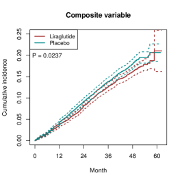
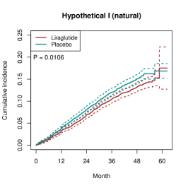
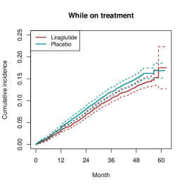
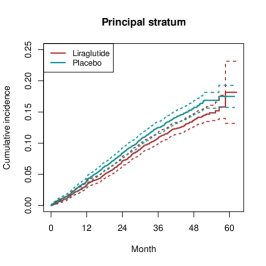
Figure 1: Estimated cumulative incidences in Study I, with 95% confidence intervals.

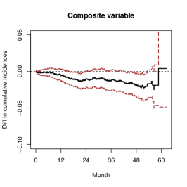
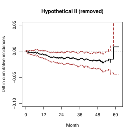
Figure 2: Estimated treatment effects in Study I, with 95% confidence intervals.

As expected, the cumulative incidences achieve the highest under the composite variable strategy, because the composite variable strategy considers the summarized occurrence of either primary outcome or intercurrent events. Of note, the cumulative incidences under the principal stratum strategy are considerably higher than those under the while on treatment strategy because the former equals the cumulative incidence of the latter divided by a factor of smaller than 1 (see §3.6). The cumulative incidence curves in hypothetical scenario II are higher than those in hypothetical scenario I. Recall in the former we set the hazard of intercurrent events at zero while in the latter we only control the hazards of intercurrent events at the same level under two treatment conditions (see §3.5). The at-risk sets in the former would be larger as some individuals who experienced intercurrent events could be maintained in the at-risk sets in the hypothetical scenario, so higher cumulative incidences are attained. The cumulative incidence curve under placebo in hypothetical scenario I is identical to that in the while on treatment strategy, confirming the earlier arguments in §3.5.

7 Discussion

The presence of intercurrent events has posed challenges in the statistical analysis for clinical trials with time-to-event outcomes. In this paper, we construct the causal estimands and provide their estimators under the five strategies in ICH E9 (R1) addendum. The treatment effect is depicted by a time-varying treatment effect curve and hypothesis tests. From the causal inference perspective, these strategies address different scientific questions and may require different data to investigate. As highlighted in the addendum, appropriate choices of strategies depend on the specific scientific question that practitioners aim to answer. Some strategies may be hard to interpret or guide practitioners in clinical practice. For example, the hypothetical strategy invisions a hypothetical scenario instead of directly exploring association using observed data, and the principal stratum strategy defines a causal effect in an unidentified target population. Therefore, drawing a meaningful causal conclusion requires discussion between statisticians and clinicians. From the regulatory perspective, the effectiveness of a drug can be reported from the estimated treatment effects at selected time points with variance and $p$-value under a specific strategy.

There are some alternatives of causal estimands apart from the difference of cumulative incidences. Generally, estimands should be defined as contrast of functionals of potential outcomes on a well-defined target population. Causal interpretations of such kind of estimands may rely on specific context as well as some implications. For example, the average hazards ratio (AHR) integrates the ratio of hazards under the treated and under the control from treatment initiation to some time point $t$ (Kalbfleisch and Prentice,, 1981; Martinussen et al.,, 2020; Prentice and Aragaki,, 2022), and the restricted mean time lost (RMTL) measures the survival time lost (or gained) by receiving active treatment compared to control in the time period from treatment initiation to some time point $t$ (Uno et al.,, 2015; Zhao et al.,, 2016). Summarizing the treatment effect to a scaler provides convenience for inference and decision making, although some information is lost. The five strategies in ICH E9 (R1) still apply to account for intercurrent events in these types of estimands.

In estimation, we focused on completely randomized clinical trials where covariates are naturally balanced between treatment groups. However, our proposed methods can be extended to incorporate covariates to handle stratified randomized experiments or observational studies (real-world data) with ignorable treatment assignment mechanism. With imbalanced covariates, we could use semiparametric models like proportional hazards and additive hazards models to estimate the hazard functions (Fine and Gray,, 1999; Robins and Finkelstein,, 2000; Abbring and Van den Berg,, 2003; Lu and Liang,, 2008; Wang et al.,, 2017; Dukes et al.,, 2019). Alternatively, we might employ propensity-score-based methods, such as generalized Kaplan-Meier or generalized Nelson-Aalen estimators or propensity score matching (Xie and Liu,, 2005; Sugihara,, 2010; Austin,, 2014; Mao et al.,, 2018). G-formula and doubly robust estimation are also available considering propensity scores and failure time models simultaneously (Robins,, 1986, 1997; Zhang and Schaubel,, 2012). The variability of estimated nuisance models should be taken into consideration to investigate the asymptotics of estimators and to construct confidence intervals, which could be of theoretical challenge. In Supplementary Material D, we provide semiparametric estimation approaches based on efficient influence functions which enjoy efficiency and robustness.

Software

The R codes are available from GitHub and CRAN upon acceptance.

Data availability statement

The data that support the findings of this study are available from Novo Nordisk A/S. Restrictions apply to the availability of these data, which were used under license for this study.

Conflict of interest

Xiao-Hua Zhou receives funding from Novo Nordisk A/S.

See pages 1-12 of SupplementaryMaterial0126.pdf

References

- Aalen, (1978) Aalen, O. (1978). Nonparametric inference for a family of counting processes. The Annals of Statistics, 6(4):701–726.
- Aalen et al., (2015) Aalen, O. O., Cook, R. J., and Røysland, K. (2015). Does Cox analysis of a randomized survival study yield a causal treatment effect? Lifetime Data Analysis, 21(4):579–593.
- Abbring and Van den Berg, (2003) Abbring, J. H. and Van den Berg, G. J. (2003). The identifiability of the mixed proportional hazards competing risks model. Journal of the Royal Statistical Society: Series B (Statistical Methodology), 65(3):701–710.
- Andersen et al., (2012) Andersen, P. K., Geskus, R. B., de Witte, T., and Putter, H. (2012). Competing risks in epidemiology: Possibilities and pitfalls. International Journal of Epidemiology, 41(3):861–870.
- Austin, (2014) Austin, P. C. (2014). The use of propensity score methods with survival or time-to-event outcomes: Reporting measures of effect similar to those used in randomized experiments. Statistics in Medicine, 33(7):1242–1258.
- Austin et al., (2016) Austin, P. C., Lee, D. S., and Fine, J. P. (2016). Introduction to the analysis of survival data in the presence of competing risks. Circulation, 133(6):601–609.
- Bornkamp et al., (2021) Bornkamp, B., Rufibach, K., Lin, J., Liu, Y., Mehrotra, D. V., Roychoudhury, S., Schmidli, H., Shentu, Y., and Wolbers, M. (2021). Principal stratum strategy: Potential role in drug development. Pharmaceutical Statistics, 20(4):737–751.
- Breum et al., (2024) Breum, M. S., Munch, A., Gerds, T. A., and Martinussen, T. (2024). Estimation of separable direct and indirect effects in a continuous-time illness-death model. Lifetime Data Analysis, pages 143–180.
- Broglio and Berry, (2009) Broglio, K. R. and Berry, D. A. (2009). Detecting an overall survival benefit that is derived from progression-free survival. JNCI: Journal of the National Cancer Institute, 101(23):1642–1649.
- Bühler et al., (2023) Bühler, A., Cook, R. J., and Lawless, J. F. (2023). Multistate models as a framework for estimand specification in clinical trials of complex processes. Statistics in Medicine, 42(9):1368–1397.
- Coemans et al., (2022) Coemans, M., Verbeke, G., Döhler, B., Süsal, C., and Naesens, M. (2022). Bias by censoring for competing events in survival analysis. BMJ, 378.
- Cole et al., (1996) Cole, B. F., Gelber, R. D., Kirkwood, J. M., Goldhirsch, A., Barylak, E., and Borden, E. (1996). Quality-of-life-adjusted survival analysis of interferon alfa-2b adjuvant treatment of high-risk resected cutaneous melanoma: An eastern cooperative oncology group study. Journal of Clinical Oncology, 14(10):2666–2673.
- Comment et al., (2019) Comment, L., Mealli, F., Haneuse, S., and Zigler, C. (2019). Survivor average causal effects for continuous time: A principal stratification approach to causal inference with semicompeting risks. arXiv preprint arXiv:1902.09304.
- Conner and Trinquart, (2021) Conner, S. C. and Trinquart, L. (2021). Estimation and modeling of the restricted mean time lost in the presence of competing risks. Statistics in Medicine, 40(9):2177–2196.
- Cox, (1972) Cox, D. R. (1972). Regression models and life-tables. Journal of the Royal Statistical Society: Series B (Methodological), 34(2):187–202.
- Cro et al., (2022) Cro, S., Kahan, B. C., Rehal, S., Ster, A. C., Carpenter, J. R., White, I. R., and Cornelius, V. R. (2022). Evaluating how clear the questions being investigated in randomised trials are: Systematic review of estimands. BMJ, 378.
- Deng et al., (2023) Deng, Y., Wang, Y., and Zhou, X.-H. (2023). Direct and indirect treatment effects in the presence of semi-competing risks. arXiv preprint arXiv:2309.01721.
- Ding and Lu, (2017) Ding, P. and Lu, J. (2017). Principal stratification analysis using principal scores. Journal of the Royal Statistical Society Series B: Statistical Methodology, 79(3):757–777.
- Dukes et al., (2019) Dukes, O., Martinussen, T., Tchetgen Tchetgen, E. J., and Vansteelandt, S. (2019). On doubly robust estimation of the hazard difference. Biometrics, 75(1):100–109.
- Emura et al., (2020) Emura, T., Shih, J.-H., Ha, I. D., and Wilke, R. A. (2020). Comparison of the marginal hazard model and the sub-distribution hazard model for competing risks under an assumed copula. Statistical Methods in Medical Research, 29(8):2307–2327.
- Fine and Gray, (1999) Fine, J. P. and Gray, R. J. (1999). A proportional hazards model for the subdistribution of a competing risk. Journal of the American Statistical Association, 94(446):496–509.
- Fine et al., (2001) Fine, J. P., Jiang, H., and Chappell, R. (2001). On semi-competing risks data. Biometrika, 88(4):907–919.
- Fleming et al., (2009) Fleming, T. R., Rothmann, M. D., and Lu, H. L. (2009). Issues in using progression-free survival when evaluating oncology products. Journal of Clinical Oncology, 27(17):2874.
- Frangakis and Rubin, (2002) Frangakis, C. E. and Rubin, D. B. (2002). Principal stratification in causal inference. Biometrics, 58(1):21–29.
- Gao et al., (2022) Gao, F., Xia, F., and Chan, K. C. G. (2022). Defining and estimating subgroup mediation effects with semi-competing risks data. Statistica Sinica.
- Geskus, (2011) Geskus, R. B. (2011). Cause-specific cumulative incidence estimation and the Fine and Gray model under both left truncation and right censoring. Biometrics, 67(1):39–49.
- Geskus, (2015) Geskus, R. B. (2015). Data analysis with competing risks and intermediate states. CRC Press.
- Gilbert et al., (2003) Gilbert, P. B., Bosch, R. J., and Hudgens, M. G. (2003). Sensitivity analysis for the assessment of causal vaccine effects on viral load in hiv vaccine trials. Biometrics, 59(3):531–541.
- Goldhirsch et al., (1989) Goldhirsch, A., Gelber, R. D., Simes, R. J., Glasziou, P., and Coates, A. S. (1989). Costs and benefits of adjuvant therapy in breast cancer: A quality-adjusted survival analysis. Journal of Clinical Oncology, 7(1):36–44.
- Gooley et al., (1999) Gooley, T. A., Leisenring, W., Crowley, J., and Storer, B. E. (1999). Estimation of failure probabilities in the presence of competing risks: New representations of old estimators. Statistics in Medicine, 18(6):695–706.
- Gray, (1988) Gray, R. J. (1988). A class of K-sample tests for comparing the cumulative incidence of a competing risk. The Annals of Statistics, 16(3):1141–1154.
- Han and Zhou, (2023) Han, S. and Zhou, X.-H. (2023). Defining estimands in clinical trials: A unified procedure. Statistics in Medicine, 42(12):1869–1887.
- Huang, (2021) Huang, Y.-T. (2021). Causal mediation of semicompeting risks. Biometrics, 77(4):1143–1154.
- International Conference on Harmonization, (2019) International Conference on Harmonization (2019). ICH E9 (R1): Addendum to statistical principles for clinical trials on choosing appropriate estimands and defining sensitivity analyses in clinical trials. (Step 4 version dated 20 Novemenber 2019). International Conference on Harmonization.
- Ionan et al., (2023) Ionan, A. C., Paterniti, M., Mehrotra, D. V., Scott, J., Ratitch, B., Collins, S., Gomatam, S., Nie, L., Rufibach, K., and Bretz, F. (2023). Clinical and statistical perspectives on the ICH E9 (R1) estimand framework implementation. Statistics in Biopharmaceutical Research, 15(2):554–559.
- Kahan et al., (2020) Kahan, B. C., Morris, T. P., White, I. R., Tweed, C. D., Cro, S., Dahly, D., Pham, T. M., Esmail, H., Babiker, A., and Carpenter, J. R. (2020). Treatment estimands in clinical trials of patients hospitalised for COVID-19: Ensuring trials ask the right questions. BMC Medicine, 18(1):1–8.
- Kalbfleisch and Prentice, (1981) Kalbfleisch, J. D. and Prentice, R. L. (1981). Estimation of the average hazard ratio. Biometrika, 68(1):105–112.
- Kaplan and Meier, (1958) Kaplan, E. L. and Meier, P. (1958). Nonparametric estimation from incomplete observations. Journal of the American Statistical Association, 53(282):457–481.
- Lambert et al., (2017) Lambert, P. C., Wilkes, S. R., and Crowther, M. J. (2017). Flexible parametric modelling of the cause-specific cumulative incidence function. Statistics in medicine, 36(9):1429–1446.
- Lange and Hansen, (2011) Lange, T. and Hansen, J. V. (2011). Direct and indirect effects in a survival context. Epidemiology, 22(4):575–581.
- Latouche et al., (2013) Latouche, A., Allignol, A., Beyersmann, J., Labopin, M., and Fine, J. P. (2013). A competing risks analysis should report results on all cause-specific hazards and cumulative incidence functions. Journal of Clinical Epidemiology, 66(6):648–653.
- Lau et al., (2009) Lau, B., Cole, S. R., and Gange, S. J. (2009). Competing risk regression models for epidemiologic data. American Journal of Epidemiology, 170(2):244–256.
- Lin et al., (1998) Lin, D., Oakes, D., and Ying, Z. (1998). Additive hazards regression with current status data. Biometrika, 85(2):289–298.
- Lipkovich et al., (2020) Lipkovich, I., Ratitch, B., and Mallinckrodt, C. H. (2020). Causal inference and estimands in clinical trials. Statistics in Biopharmaceutical Research, 12(1):54–67.
- Lu and Liang, (2008) Lu, W. and Liang, Y. (2008). Analysis of competing risks data with missing cause of failure under additive hazards model. Statistica Sinica, 18:219–234.
- Mao et al., (2018) Mao, H., Li, L., Yang, W., and Shen, Y. (2018). On the propensity score weighting analysis with survival outcome: Estimands, estimation, and inference. Statistics in Medicine, 37(26):3745–3763.
- Marso et al., (2016) Marso, S. P., Daniels, G. H., Brown-Frandsen, K., Kristensen, P., Mann, J. F., Nauck, M. A., Nissen, S. E., Pocock, S., Poulter, N. R., Ravn, L. S., et al. (2016). Liraglutide and cardiovascular outcomes in type 2 diabetes. New England Journal of Medicine, 375(4):311–322.
- Martinussen and Stensrud, (2021) Martinussen, T. and Stensrud, M. J. (2021). Estimation of separable direct and indirect effects in continuous time. Biometrics.
- Martinussen and Stensrud, (2023) Martinussen, T. and Stensrud, M. J. (2023). Estimation of separable direct and indirect effects in continuous time. Biometrics, 79(1):127–139.
- Martinussen and Vansteelandt, (2013) Martinussen, T. and Vansteelandt, S. (2013). On collapsibility and confounding bias in Cox and Aalen regression models. Lifetime Data Analysis, 19(3):279–296.
- Martinussen et al., (2020) Martinussen, T., Vansteelandt, S., and Andersen, P. K. (2020). Subtleties in the interpretation of hazard contrasts. Lifetime Data Analysis, 26:833–855.
- Martinussen et al., (2011) Martinussen, T., Vansteelandt, S., Gerster, M., and Hjelmborg, J. v. B. (2011). Estimation of direct effects for survival data by using the aalen additive hazards model. Journal of the Royal Statistical Society: Series B (Statistical Methodology), 73(5):773–788.
- Nelson, (1972) Nelson, W. (1972). Theory and applications of hazard plotting for censored failure data. Technometrics, 14(4):945–966.
- Nevo and Gorfine, (2022) Nevo, D. and Gorfine, M. (2022). Causal inference for semi-competing risks data. Biostatistics, 23(4):1115–1132.
- Pintilie, (2007) Pintilie, M. (2007). Analysing and interpreting competing risk data. Statistics in Medicine, 26(6):1360–1367.
- Prentice and Aragaki, (2022) Prentice, R. L. and Aragaki, A. K. (2022). Intention-to-treat comparisons in randomized trials. Statistical Science, 37(3):380–393.
- Ratitch et al., (2020) Ratitch, B., Bell, J., Mallinckrodt, C., Bartlett, J. W., Goel, N., Molenberghs, G., O’Kelly, M., Singh, P., and Lipkovich, I. (2020). Choosing estimands in clinical trials: Putting the ICH E9 (R1) into practice. Therapeutic Innovation & Regulatory Science, 54(2):324–341.
- Revicki et al., (2006) Revicki, D. A., Feeny, D., Hunt, T. L., and Cole, B. F. (2006). Analyzing oncology clinical trial data using the Q-TWiST method: Clinical importance and sources for health state preference data. Quality of Life Research, 15(3):411–423.
- Robins, (1986) Robins, J. (1986). A new approach to causal inference in mortality studies with a sustained exposure period — application to control of the healthy worker survivor effect. Mathematical Modelling, 7(9-12):1393–1512.
- Robins, (1997) Robins, J. M. (1997). Causal inference from complex longitudinal data. In Latent Variable Modeling and Applications to Causality, pages 69–117. Springer.
- Robins and Finkelstein, (2000) Robins, J. M. and Finkelstein, D. M. (2000). Correcting for noncompliance and dependent censoring in an AIDS clinical trial with inverse probability of censoring weighted (IPCW) log-rank tests. Biometrics, 56(3):779–788.
- Robins and Greenland, (1992) Robins, J. M. and Greenland, S. (1992). Identifiability and exchangeability for direct and indirect effects. Epidemiology, 3(2):143–155.
- Rubin, (1974) Rubin, D. B. (1974). Estimating causal effects of treatments in randomized and nonrandomized studies. Journal of Educational Psychology, 66(5):688.
- Rubin, (1980) Rubin, D. B. (1980). Randomization analysis of experimental data: The Fisher randomization test comment. Journal of the American Statistical Association, 75(371):591–593.
- Siegel et al., (2022) Siegel, J. M., Weber, H.-J., and Englert, S. (2022). The role of occlusion: Potential extension of the ICH E9 (R1) addendum on estimands and sensitivity analysis for time-to-event oncology studies. arXiv preprint arXiv:2203.02182.
- Stuart and Jo, (2015) Stuart, E. A. and Jo, B. (2015). Assessing the sensitivity of methods for estimating principal causal effects. Statistical Methods in Medical Research, 24(6):657–674.
- Sugihara, (2010) Sugihara, M. (2010). Survival analysis using inverse probability of treatment weighted methods based on the generalized propensity score. Pharmaceutical Statistics: The Journal of Applied Statistics in the Pharmaceutical Industry, 9(1):21–34.
- Tchetgen Tchetgen, (2011) Tchetgen Tchetgen, E. J. (2011). On causal mediation analysis with a survival outcome. The International Journal of Biostatistics, 7(1).
- Uno et al., (2015) Uno, H., Wittes, J., Fu, H., Solomon, S. D., Claggett, B., Tian, L., Cai, T., Pfeffer, M. A., Evans, S. R., and Wei, L.-J. (2015). Alternatives to hazard ratios for comparing the efficacy or safety of therapies in noninferiority studies. Annals of Internal Medicine, 163(2):127–134.
- Wang et al., (2023) Wang, C., Zhang, Y., Mealli, F., and Bornkamp, B. (2023). Sensitivity analyses for the principal ignorability assumption using multiple imputation. Pharmaceutical Statistics, 22(1):64–78.
- Wang et al., (2017) Wang, Y., Lee, M., Liu, P., Shi, L., Yu, Z., Awad, Y. A., Zanobetti, A., and Schwartz, J. D. (2017). Doubly robust additive hazards models to estimate effects of a continuous exposure on survival. Epidemiology, 28(6):771.
- Wei, (1992) Wei, L.-J. (1992). The accelerated failure time model: A useful alternative to the Cox regression model in survival analysis. Statistics in Medicine, 11(14-15):1871–1879.
- Winnett and Sasieni, (2002) Winnett, A. and Sasieni, P. (2002). Adjusted Nelson–Aalen estimates with retrospective matching. Journal of the American Statistical Association, 97(457):245–256.
- Xie and Liu, (2005) Xie, J. and Liu, C. (2005). Adjusted Kaplan–Meier estimator and log-rank test with inverse probability of treatment weighting for survival data. Statistics in Medicine, 24(20):3089–3110.
- Xu et al., (2010) Xu, J., Kalbfleisch, J. D., and Tai, B. (2010). Statistical analysis of illness–death processes and semicompeting risks data. Biometrics, 66(3):716–725.
- Xu et al., (2022) Xu, Y., Scharfstein, D., Müller, P., and Daniels, M. (2022). A bayesian nonparametric approach for evaluating the causal effect of treatment in randomized trials with semi-competing risks. Biostatistics, 23(1):34–49.
- (77) Young, B. E., Ong, S. W. X., Kalimuddin, S., Low, J. G., Tan, S. Y., Loh, J., Ng, O.-T., Marimuthu, K., Ang, L. W., Mak, T. M., et al. (2020a). Epidemiologic features and clinical course of patients infected with SARS-CoV-2 in singapore. JAMA, 323(15):1488–1494.
- (78) Young, J. G., Stensrud, M. J., Tchetgen Tchetgen, E. J., and Hernán, M. A. (2020b). A causal framework for classical statistical estimands in failure-time settings with competing events. Statistics in Medicine, 39(8):1199–1236.
- Zhang and Schaubel, (2012) Zhang, M. and Schaubel, D. E. (2012). Contrasting treatment-specific survival using double-robust estimators. Statistics in Medicine, 31(30):4255–4268.
- Zhao et al., (2016) Zhao, L., Claggett, B., Tian, L., Uno, H., Pfeffer, M. A., Solomon, S. D., Trippa, L., and Wei, L. (2016). On the restricted mean survival time curve in survival analysis. Biometrics, 72(1):215–221.