GCBF+: A Neural Graph Control Barrier Function Framework for Distributed Safe Multi-Agent Control

Abstract

Distributed, scalable, and safe control of large-scale multi-agent systems (MAS) is a challenging problem. In this paper, we design a distributed framework for safe multi-agent control in large-scale environments with obstacles, where a large number of agents are required to maintain safety using only local information and reach their goal locations. We introduce a new class of certificates, termed graph control barrier function (GCBF), which are based on the well-established control barrier function (CBF) theory for safety guarantees and utilize a graph structure for scalable and generalizable distributed control of MAS. We develop a novel theoretical framework to prove the safety of an arbitrary-sized MAS with a single GCBF. We propose a new training framework GCBF+ that uses graph neural networks (GNNs) to parameterize a candidate GCBF and a distributed control policy. The proposed framework is distributed and is capable of directly taking point clouds from LiDAR, instead of actual state information, for real-world robotic applications. We illustrate the efficacy of the proposed method through various hardware experiments on a swarm of drones with objectives ranging from exchanging positions to docking on a moving target without collision. Additionally, we perform extensive numerical experiments, where the number and density of agents, as well as the number of obstacles, increase. Empirical results show that in complex environments with nonlinear agents (e.g., Crazyflie drones) GCBF+ outperforms the handcrafted CBF-based method with the best performance by up to $20\%$ for relatively small-scale MAS for up to 256 agents, and leading reinforcement learning (RL) methods by up to $40\%$ for MAS with 1024 agents. Furthermore, the proposed method does not compromise on the performance, in terms of goal reaching, for achieving high safety rates, which is a common trade-off in RL-based methods.

I Introduction

I-A Background

Multi-agent systems (MAS) have received tremendous attention from scholars in different disciplines, including computer science and robotics, as a means to solve complex problems by subdividing them into smaller tasks [1]. MAS applications include but are not limited to warehouse operations [2, 3], self-driving cars [4, 5, 6, 7], coordinated navigation of a swarm of drones in a dense forest for search-and-rescue missions [8, 9]; interested reader is referred to [10] for an overview of MAS applications. For such safety-critical MASs, it is important to design controllers that not only guarantee safety in terms of collision and obstacle avoidance but are also scalable to large-scale multi-agent problems.

Common MAS motion planning methods include but are not limited to solving mixed integer linear programs (MILP) for computing safe paths for agents [11, 12] and sampling-based planning methods such as rapidly exploring random tree (RRT) [13]. However, such centralized approaches, where the complete MAS state information is used, are not scalable to large-scale MAS. The recent work [14] performing distributed trajectory optimization proposes a scalable method for MAS control. However, this approach cannot take into account changing neighborhoods and environments, limiting its applications. There has been quite a lot of development in the learning-based methods for MAS control in recent years; see [15] for a detailed overview of learning-based methods for safe control of MAS. Multi-agent Reinforcement Learning (MARL)-based approaches, e.g., Multi-agent Proximal Policy Optimization (MAPPO) [16], have also been adapted to solve multi-agent motion planning problems. However, when it comes to RL, one main challenge for safety, particularly in multi-agent cases, is the tradeoff between the practical performance and the safety requirement because of the conflicting reward-penalty structure [15]. We argue that our proposed framework does not suffer from a similar tradeoff and can automatically balance satisfying safety requirements and performance criteria through a carefully designed training loss.

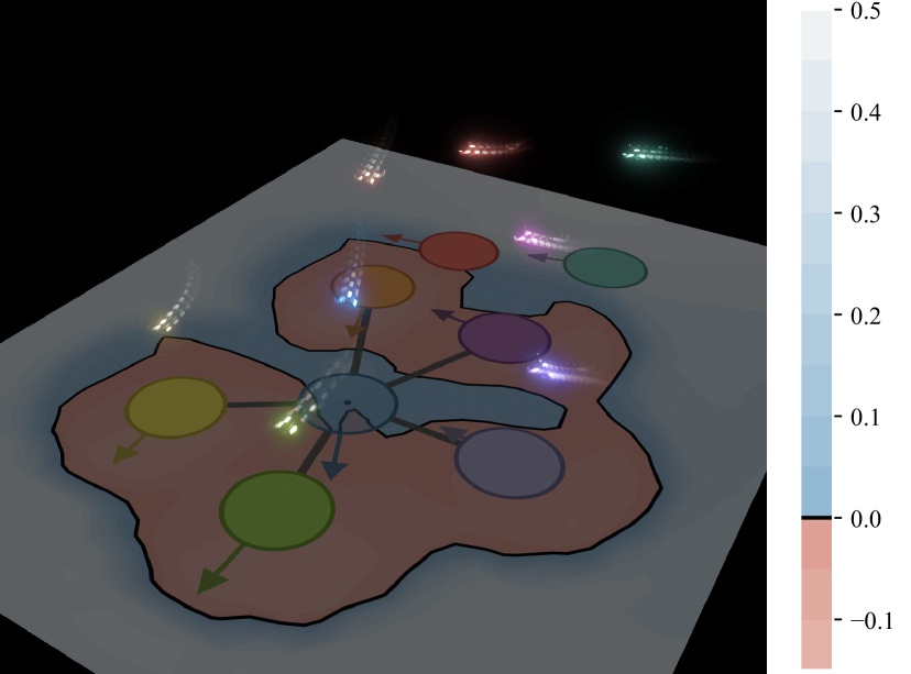
Figure 1: 8-Crazyflie swapping with GCBF: We learn a decentralized graph control barrier function (GCBF) for an 8-agent swapping task on the Crazyflie hardware platform. We visualize the learned GCBF for the blue agent and draw the edges with its neighboring agents in grey. The learned GCBF can handle arbitrary graph topologies and hence can scale to an arbitrary number of agents without retraining.

Traditionally, for robotic systems, control barrier functions (CBFs) have become a popular tool to encode safety requirements [17]. CBF-based quadratic programs (QPs) have gained popularity for control synthesis as QPs can be solved efficiently for single-agent systems, or small-scale MAS for real-time control synthesis [18]. For MAS, safety is generally formulated pair-wise and a CBF is assigned for each pair-wise safety constraint, and then an approximation method is used to combine multiple constraints [19, 20, 21, 22]. While hand-crafted CBF-QPs have shown promising results when it comes to the safety of single-agent systems [18] and simple small-scale multi-agent systems [23], it is difficult to find a CBF when it comes to highly complex nonlinear systems and large-scale MAS. Another major challenge in such approaches is constructing a CBF in the presence of input constraints, e.g. actuation limits. There are some recent developments in this area [24, 25, 26] with extensions to MAS in [27]; however, as also noted by the authors in [24], finding a function that satisfies these conditions is a complex problem.

I-B Our contributions

To overcome these limitations, in this paper, we first introduce the notion of graph control barrier function, termed GCBF, for large-scale MAS to address the problems of safety, scalability, and generalizability. The proposed GCBF architecture can account for arbitrary and changing number of neighbors, and hence, is applicable to large-scale MAS. We prove that the existence of a GCBF guarantees safety in an MAS. We provide a new safety result using the notion of GCBF that guarantees the safety of MAS of arbitrary size. This is the first such result that shows the safety of MAS of any size using one barrier function. Next, we introduce GCBF+, a novel training framework to learn a candidate GCBF along with a distributed control policy. We use graph neural networks (GNNs) to better capture the changing graphical topology of distance-based inter-agent communications. We propose a novel loss function formulation that accounts for safety, goal-reaching as well as actuation limits, thereby addressing all the major limitations of hand-crafted CBF-QP methods. Furthermore, the proposed algorithm can work with LiDAR-based point-cloud observations to handle obstacles in real-world environments. With these technologies, our proposed framework can generalize well to many challenging settings, including crowded and unseen obstacle environments.

We perform various hardware experiments on a swarm of Crazyflie drones to corroborate the practical applicability of the proposed framework. The hardware experiments consist of the drones safely exchanging positions in a crowded workspace in the presence of a moving obstacle and docking on a moving target while maintaining safety. We also perform extensive numerical experiments and provide empirical evidence of the improved performance of the proposed GCBF+ framework compared to the prior version of the algorithm (GCBFv0) in [28], a state-of-the-art MARL method (InforMARL) [29], and hand-crafted CBF-QP methods from [23]. We consider three 2D environments and two 3D environments in our numerical experiments consisting of linear and nonlinear systems. In the obstacle-free case, we train with 8 agents and test with over 1000 agents. In the linear cases, the performance improvement (in terms of safety rate) is of the order of 5%, while in the nonlinear cases, the performance improvement is more than 30%. In the obstacle environment, we consider only 8 obstacles in training, while in testing, we consider up to 128 obstacles. These experiments corroborate that the proposed method outperforms the baseline methods in successfully completing the tasks in various 2D and 3D environments.

I-C Differences from conference version

This paper builds on the conference paper [28] which presented the GCBFv0 algorithm. We propose a new algorithm GCBF+ which improves upon GCBFv0 in the following ways.

• Algorithmic modifications: In the prior work, the control policy was learned to account only for the safety constraints, and a CBF-based switching mechanism was used for switching between a goal-reaching nominal controller and a safe neural controller. This led to undesirable behavior and deadlocks in certain situations. Furthermore, an online policy refinement mechanism was used in [28] when the learned controller was unable to satisfy the safety requirements which required agents to communicate their control actions for the policy update, adding computational overhead. We modify the way the training loss is defined so that the safety and the goal-reaching requirements do not conflict with each other, making it possible for the training loss to go to zero. In this way, we can use a single controller for both safety and goal-reaching, without an online policy refinement step for higher safety rates.

• Actuation limits  Another major limitation of GCBFv0 is that it does not account for actuator limits which may result in undesirable behavior when implemented on real-world robotic systems. In contrast, in the proposed method in this work, the learned controller takes into account actuator limits through a look-ahead mechanism for approximation of the safe control invariant set. This mechanism ensures that the learned controller satisfies the actuation limits while keeping the system safe.

• Theoretical results on generalization  While [28] proves that a GBCF guarantees safety for a specific size of the MAS, it does not prove that the same GCBF can also guarantee safety when the number of agents changes. We advance this theoretical result to prove that a GCBF can certify the safety of a MAS of any size. This brings the theoretical understanding of the algorithm closer to the empirical results, where we observe the new GCBF+ algorithm can scale to over $1000$ agents despite being trained with $8$ agents.

• Hardware experiments  We include various hardware experiments on a swarm of Crazyflie drones, thereby demonstrating the practicality of the proposed framework.

• Additional numerical experiments  We also include various new numerical experiments as compared to the conference version. In particular, we perform experiments with more realistic system dynamics, such as the 6DOF Crazyflie drone, in contrast to simpler dynamics used in the numerical experiments in [28]. Furthermore, we provide comparisons to new baselines: InforMARL from [29], which is a better RL-based method for safe MAS control, and centralized and distributed hand-crafted CBF-based methods from [23].

• Better performance   We illustrate that the new GCBF+ algorithm proposed in this paper has much better performance than the original GCBFv0 algorithm in the conference version. In particular, in complex environments consisting of nonlinear agents, GCBFv0 has a success rate of less than $10\%$ while GCBF+ has a success rate of over $55\%$. Furthermore, in crowded 2D obstacle environments, GCBFv0 has a success rate close to $20\%$ while GCBF+ has a success rate of over $95\%$.

I-D Related work

Graph-based methods  Graph-based planning approaches such as prioritized multi-agent path finding (MAPF) [30] and conflict-based search for MAPF [31] can be used for multi-agent path planning for known environments. However, MAPF do not take into account system dynamics, and do not scale to large-scale systems due to computational complexity. Another line of work for motion planning in obstacle environments is based on the notion of velocity obstacles [32] defined using collision cones for velocity. Such methods can be used for large-scale systems with safety guarantees under mild assumptions. However, the current frameworks under this notion assume single or double integrator dynamics for agents. The work in [33] scales to large-scale systems, but it only considers a discrete action space and hence does not apply to robotic platforms that use more general continuous input signals.

Centralized CBF-based methods   For systems with relatively simple dynamics, such as single integrator, double integrator, and unicycle dynamics, it is possible to use a distance-based CBF [17]. For systems with polynomial dynamics, it is possible to use the Sum-of-Squares (SoS) [34] method to compute a CBF [35]. The key idea of SoS is that the CBF conditions consist of a set of inequalities, which can be equivalently expressed as checking whether a polynomial function is SoS. In this manner, a CBF can be computed through convex optimization [35, 36, 37]. However, the SoS-based approaches suffer from the curse of dimensionality (i.e., the computational complexity grows exponentially with the degree of polynomials involved) [38].

Distributed CBF-based methods   While centralized CBF is an effective shield for small-scale MAS, due to its poor scalability, it is difficult to use it for large-scale MAS. To address the scalability problem, the notion of distributed CBF can be used [23, 28, 39, 40]. In contrast to centralized CBF where the state of the MAS is used, for a distributed CBF, only the local observations and information available from communication with neighbors are used, reducing the problem dimension significantly.

Learning CBFs  One way of navigating the challenge of hand-crafting a CBF is to use neural networks (NNs) for learning a CBF [41]. In the past few years, machine learning (ML)-based methods have been used to learn CBFs for complex systems [42, 40, 43, 44, 45, 46] . However, it is challenging for them to balance safety and task performance for multi-task problems, and some methods are not scalable to large-scale multi-agent problems. The Multi-agent Decentralized CBF (MDCBF) framework in [40] uses an NN-based CBF designed for MAS. However, they do not encode a method of distinguishing between other controlled agents and uncontrolled agents such as static and dynamic obstacles. This can lead to either conservative behaviors if all the neighbors are treated as non-cooperative obstacles, or collisions if the obstacles are treated as cooperative, controlled agents. Furthermore, the method in [40] does not account for changing graph topology in their approximation, which can lead to an incorrect evaluation of the CBF constraints and consequently, failure.

Multi-agent RL   The review paper [47] provides a good overview of the recent developments in multi-agent RL (MARL) with applications in safe control design (see [48, 49, 50]). There is also a lot of work on MARL-based approaches with focuses on motion planning [16, 51, 52, 53, 39, 54]. However, these approaches do not provide safety guarantees due to the reward structure. One major challenge with MARL is designing a reward function for MAS that balances safety and performance. As argued in [55], MARL-based methods are still in the initial phase of development when it comes to safe multi-agent motion planning.

GNN-based methods   Utilizing the permutation-invariance property, GNN-based methods have been employed for problems involving MAS [56, 57, 58, 59, 60, 61]. The Control Admissiblity Models (CAM)-based framework in [56] uses a GNN framework for safe control design for MAS. However, it involves sampling control actions from a set defined by CAM and there are no guarantees that such a set is non-empty, leading to feasibility-related issues of the approach. Works such as [57, 62] use GNNs for generalization to unseen environments and are shown to work on teams of up to a hundred agents. However, in the absence of an attention mechanism, the computational cost grows with the number of agents in the neighborhood and hence, these methods are not scalable to very large-scale problems (e.g., a team of 1000 agents) due to the computational bottleneck.

The rest of this article is organized as follows. We formulate the MAS control problem in Section II. Then, we present GCBF as a safety certificate for MAS in Section III, and the framework for learning GCBF and a distributed control policy in Section IV. Section V presents the implementation details on the proposed method, while Sections VI and VII present numerical and hardware experimental results, respectively. Section VIII presents the conclusions of the paper, discusses the limitations of the proposed framework, and proposes directions for future work.

II Problem formulation

Notations  In the rest of the paper, $\mathbb{R}$ denotes the set of real numbers and $\mathbb{R}_{+}$ denotes the set of non-negative real numbers. We use $\|\cdot\|$ to denote the Euclidean norm. A continuous function $\alpha:\mathbb{R}_{+}\rightarrow\mathbb{R}_{+}$ is a class-$\mathcal{K}$ function if it is strictly increasing and $\alpha(0)=0$. It belongs to $\mathcal{K}_{\infty}$ if in addition, $\lim\limits_{r\to\infty}\alpha(r)=\infty$ and extended $\mathcal{K}_{\infty}$ if its domain and range is $\mathbb{R}$. We use $[\cdot]_{+}$ to denote the function $\max(0,\cdot)$. We drop the arguments $t,x$ whenever clear from the context. Unless otherwise specified, given a set of vectors $\{x_{i}\}$ with $x_{i}\in\mathcal{X}$ for each $i\in 1,2,\dots N$ and an index set $\mathcal{I}$, we define $\bar{x}_{I}\in\mathcal{X}^{\left\lvert I\right\rvert}$ as the concatenated vector of the vectors $x_{i}$ with index $i\in I$ from the index set.

We consider the problem of designing a distributed control framework to drive $N$ agents, each denoted with an index from the set $V_{a}\coloneqq\{1,2,\dots,N\}$, to their goal locations in an environment with obstacles while avoiding collisions. The motion of each agent is governed by general nonlinear control affine dynamics

$$\dot{x}_{i}=f_{i}(x_{i})+g_{i}(x_{i})u_{i},$$ (1)

where $x_{i}\in\mathcal{X}_{i}\subset\mathbb{R}^{n}$ and $u_{i}\in\mathcal{U}_{i}\subset\mathbb{R}^{m}$ are the state, control input for the $i$-th agent, respectively and $f_{i}:\mathbb{R}^{n}\rightarrow\mathbb{R}^{n},g_{i}:\mathbb{R}^{n}\rightarrow\mathbb{R}^{n\times m}$ are assumed to be locally Lipschitz continuous. Note that it is possible to consider heterogeneous MAS where the dynamics of agents are different. However, for simplicity, we restrict our discussion to the case when all agents have the same underlying dynamics, i.e., where $\mathcal{X}_{i}=\mathcal{X}$, $\mathcal{U}_{i}=\mathcal{U}$ and $f_{i}=f$, $g_{i}=g$ for all $i\in V_{a}$. For convenience, we also define the motion of the entire MAS via the concatenated state vector $\bar{x}\coloneqq[x_{1};x_{2};\dots;x_{N}]\in{\mathcal{X}}^{N}$ and $\bar{u}\coloneqq[u_{1};u_{2};\dots;u_{N}]\in\mathcal{U}^{N}$, such that (1) can equivalently be expressed as

$$\dot{\bar{x}}=\bar{f}(\bar{x})+\bar{g}(\bar{x})\bar{u},$$ (2)

with $\bar{f}$ and $\bar{g}$ defined accordingly.

Let $\mathbb{P}\subset\mathbb{R}^{\mathfrak{n}}$ denote the set of positions in an $\mathfrak{n}$-dimensional of the environment (i.e., $\mathfrak{n}=2$ or $\mathfrak{n}=3$). We assume that each state $x\in\mathcal{X}$ is associated with a position $p\in\mathbb{P}$, and denote by $\{p_{i}\}_{i\in V_{a}}$ the first $\mathfrak{n}$ elements of $x$ corresponding to the positions of each agent. For each agent $i\in V_{a}$, we consider a goal position $p^{g}_{i}\in\mathbb{P}$, and define $\bar{p}^{g}$ as the concatenated goal vector. The observation data consists of $n_{\mathrm{rays}}>0$ evenly-spaced LiDAR rays originating from each robot and measures the relative location of obstacles within a sensing radius $R>0$. For mathematical convenience, we denote the $j$th ray from agent $i$ by $y^{(i)}_{j}\in\mathcal{X}$, where the first $\mathfrak{n}$ elements contain the position and the last $n-\mathfrak{n}$ elements are zero paddings. We then denote the aggregated rays as $\bar{y}_{i}\coloneqq[y_{1}^{(i)};\dots;y_{n_{\mathrm{rays}}}^{(i)}]\in\mathcal{X}^{n_{\mathrm{rays}}}$. The inter-agent collision avoidance requirement imposes that each pair of agents maintain a safety distance of $2r$ while the obstacle avoidance requirement dictates that $|y^{(i)}_{j}|>r$ for all $j=1,2,\dots,n_{\mathrm{rays}}$, where $r>0$ is the radius of a circle that can contain the entire physical body of each agent. The control objective for each agent $i$ is to navigate the obstacle-filled environment to reach its goal $p^{g}_{i}$, as described below.

Problem 1.

Design a distributed control policy $\pi_{i}$ such that, for a set of $N$ agents $\bar{x}$ and non-colliding goal locations $\bar{p}^{g}$, the following holds for the closed-loop trajectories for each agent $i\in V_{a}$.

• Safety (Obstacles): $\|y^{(i)}_{j}(t)\|>r,\;\forall j=1,\dots,n_{\mathrm{rays}}{}$, i.e., the agents do not collide with the obstacles.

• Safety (Other Agents): $\|p_{i}(t)-p_{j}(t)\|>2r$ for all $t\geq 0$, $j\neq i$, i.e., the agents do not collide with each other.

• Liveness: $\inf\limits_{t\geq 0}\|p_{i}(t)-p^{g}_{i}\|=0$, i.e., each agent eventually reaches its goal location $p^{g}_{i}$.

To solve 1, we consider the existence of a nominal controller that satisfies the liveness property but not necessarily the safety property, and construct a GCBF-based distributed control policy to additionally satisfy the safety property.

III GCBF: a safety certificate for MAS

Based on the algorithm in [28] (GCBFv0), we propose an improved algorithm, termed GCBF+, to train a graph CBF (GCBF) that encodes the collision-avoidance constraints based on the graph structure of MAS. We use GNNs to learn a candidate GCBF jointly with the collision-avoidance control policy. Our GNN architecture is capable of handling a variable number of neighbors and hence results in a distributed and scalable solution to the safe MAS control problem.

III-A Safety for arbitrary sized MAS via graphs

We first review the notion of CBF commonly used in literature for safety requirements [17]. Consider a system $\dot{x}=F(x,u)$ where $x\in\mathcal{X}\subset\mathbb{R}^{n}$, $u\in\mathcal{U}\subset\mathbb{R}^{m}$ and $F:\mathbb{R}^{n}\times\mathbb{R}^{m}\to\mathbb{R}^{n}$. Let $\mathcal{C}\subset\mathcal{X}$ be the $0$-superlevel set of a continuously differentiable function $h:\mathcal{X}\rightarrow\mathbb{R}$, i.e., $\mathcal{C}=\{x\in\mathcal{X}:h(x)\geq 0\}$. Then, $h$ is a CBF if there exists an extended class-$\mathcal{K}_{\infty}$ function $\alpha:\mathbb{R}\rightarrow\mathbb{R}$ such that:

$$\sup_{u\in\mathcal{U}}\left[\frac{\partial h}{\partial x}F(x,u)+\alpha\left(h(x)\right)\right]\geq 0,\quad\forall x\in\mathcal{X}.$$ (3)

Let $\mathcal{S}\subset\mathcal{X}$ denote a safe set with the objective that the system trajectories do not leave this set. If $\mathcal{C}\subset\mathcal{S}$, then the existence of a CBF implies the existence of a control input $u$ that keeps the system safe [18].

Based on the notion of CBF, we define the new notion of a GCBF to encode safety for MAS of any size. To do so, we first define the graph structure we will use in this work.

A directed graph is an ordered pair $G=(V,E)$, where $V$ is the set of nodes, and $E\subset\{(i,j)\mid i\in V_{a},\,j\in V\}$ is the set of edges representing the flow of information from a sender node (henceforth called a neighbor) $j$ to a receiver agent $i$. For any graph $G=(V,E)$, let $\tilde{\mathcal{N}}_{i}$ denote the set of sender nodes for agent $i\in V_{a}$. For the considered MAS, we define the set of nodes $V=V_{a}\cup V_{o}$ to consist of the agents $V_{a}$ and the hitting points of all the LiDAR rays from all agents denoted as $V_{o}$. The edges are defined between each observed point and the observing agent when the distance between them is within a sensing radius $R>2r>0$.

Given $\mathfrak{n}$, sensing radius $R$, safety radius $r$ and $n_{\mathrm{rays}}$, define $M-1\in\mathbb{N}$ as the maximum number of sender neighbors that each receiver agent node can have while all the agents in the neighborhood remain safe. To simplify the safety analysis, define $\mathcal{N}_{i}\subseteq\tilde{\mathcal{N}}_{i}$ as the set of $M$ closest neighboring nodes to agent $i$ which also includes agent $i$. Next, define $\bar{x}_{\mathcal{N}_{i}}\in\mathcal{X}^{M}$ as the concatenated vector of $x_{i}$ and the neighbor node states with fixed size $M$ that is padded with a constant vector if $\big{\lvert}\mathcal{N}_{i}\big{\rvert}<M$.

Remark 1.

We define $M$ as above so that, for $i\in V_{a}$, changes in the neighboring indices $\mathcal{N}_{i}$ can only occur without collision at a distance $R$ (see Appendix A).

III-B Graph Control Barrier Functions

We define the safe set $\mathcal{S}_{N}\subset\mathcal{X}^{N}$ of an $N$-agent MAS as the set of MAS states $\bar{x}$ that satisfy the safety properties in Problem 1, i.e.,

$$\mathcal{S}_{N}\coloneqq\Big{\{}\bar{x}\in\mathcal{X}^{N}\;\Big{|} \;\Big{(}\left\lVert y_{j}^{(i)}\right\rVert>r,\;\forall i\in V_{a},\forall j\in n_{\mathrm{rays}}\Big{)}\bigwedge$$ (4)

$$\Big{(}\min_{i,j\in V_{g},i\neq j}\left\lVert p_{i}-p_{j}\right\rVert>2r\Big{)}\Big{\}}.$$

Then, the unsafe, or avoid, set of the MAS $\mathcal{A}_{N}=\mathcal{X}^{N}\setminus\mathcal{S}_{N}$ is defined as the complement of $\mathcal{S}_{N}$. We now define the notion GCBF as follows.

Definition 1 (GCBF).

A continuously differentiable function $h:\mathcal{X}^{M}\to\mathbb{R}$ is termed as a Graph CBF (GCBF) if there exists an extended class-$\mathcal{K}_{\infty}$ function $\alpha$ and a control policy $\pi_{i}:\mathcal{X}^{M}\to\mathcal{U}$ for each agent $i\in V_{a}$ of the MAS such that, for all $\bar{x}\in\mathcal{X}^{N}$ with $N\geq M$,

$$\dot{h}(\bar{x}_{\mathcal{N}_{i}})+\alpha(h(\bar{x}_{\mathcal{N}_{i}}))\geq 0,\quad\forall i\in V_{a}$$ (5)

where

$$\dot{h}(\bar{x}_{\mathcal{N}_{i}})=\sum_{j\in\mathcal{N}_{i}}\frac{\partial h(\bar{x}_{\mathcal{N}_{i}})}{\partial x_{j}}\left(f(x_{j})+g(x_{j})u_{j}\right),$$ (6)

for $u_{j}=\pi_{j}(\bar{x}_{\mathcal{N}_{j}})$.

Assumption 1.

For a given agent $i\in V_{a}$, a neighboring node $j$ where $\left\lVert p_{i}-p_{j}\right\rVert\geq R$ does not affect the GCBF $h$. Specifically, for any neighborhood set $\mathcal{N}_{i}$, let $\mathcal{N}^{<R}_{i}$ denote the set of neighbors in $\mathcal{N}_{i}$ that are strictly inside the sensing radius $R$ as

$$\mathcal{N}^{<R}_{i}\coloneqq\{j:\left\lVert p_{i}-p_{j}\right\rVert<R,\;j\in\mathcal{N}_{i}\}.$$ (7)

Then,

1. The gradient of $h$ with respect to nodes $R$ away is $0$, i.e.,

   $$\frac{\partial h}{\partial x_{j}}(\bar{x}_{\mathcal{N}_{i}})=0,\quad\forall j\in\mathcal{N}_{i}\setminus\mathcal{N}^{<R}_{i}.$$ (8)

2. The value of $h$ does not change when restricting to neighbors that are in $\mathcal{N}^{<R}_{i}$, i.e.,

   $$h(\bar{x}_{\mathcal{N}_{i}})=h(\bar{x}_{\mathcal{N}^{<R}_{i}}).$$ (9)

Remark 2.

We impose 1 so that $t\mapsto h(\bar{x}_{\mathcal{N}_{i}}(t))$ is a continuously differentiable function despite $\bar{x}_{\mathcal{N}_{i}}(t)$ having discontinuities whenever the set of neighboring indices $\mathcal{N}_{i}(t)$ to agent $i$ changes (see Appendix B).

Remark 3.

One way of satisfying 1 is by taking $h$ to be of the form

$$h(\bar{x}_{\mathcal{N}_{i}})=\xi_{1}\bigg{(}\sum_{j\in\mathcal{N}_{i}}w(x_{i},x_{j})\,\xi_{2}(x_{i},x_{j})\bigg{)},$$ (10)

where $\xi_{1}:\mathbb{R}^{\rho}\to\mathbb{R}$ and $\xi_{2}:\mathcal{X}\times\mathcal{X}\to\mathbb{R}^{\rho}$ are two encoding functions with $\rho$ the dimension of the feature space, and $w:\mathcal{X}\times\mathcal{X}\to\mathbb{R}$ is a continuously differentiable function such that $w(x_{i},x_{j})=0$ and $\frac{\partial w}{\partial x_{j}}(x_{i},x_{j})=0$ whenever $\left\lVert p_{i}-p_{j}\right\rVert\geq R$. In practice, we use graph attention [63], which takes the form (10), to realize 1, which we introduce later in Section IV-A.

Under 1, a GCBF certifies the forward invariance of its $0$-superlevel set under a suitable choice of control inputs. For a GCBF $h$, let $\mathcal{C}_{h}\subset\mathcal{X}^{M}$ denote the $0$-superlevel set of $h$

$$\mathcal{C}_{h}\coloneqq\{\tilde{x}\in\mathcal{X}^{M}\mid h(\tilde{x})\geq 0\},$$ (11)

and define $\mathcal{C}_{N}\subset\mathcal{X}^{N}$ as the set of $N$-agent MAS states where $\bar{x}_{\mathcal{N}_{i}}$ lie inside $\mathcal{C}_{h}$ for all $i\in V_{a}$, i.e.,

$$\mathcal{C}_{N} \coloneqq\bigcap_{i=1}^{N}\mathcal{C}_{N,i},$$ (12)

where

$$\mathcal{C}_{N,i} \coloneqq\{\bar{x}\in\mathcal{X}^{N}\mid\bar{x}_{\mathcal{N}_{i}}\in\mathcal{C}_{h}\}.$$ (13)

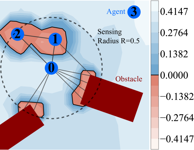
Figure 2: GCBF contours: For a fixed neighborhood $\mathcal{N}_{0}$ of agent $0$, we plot the contours of the learned GCBF $h_{\theta}$ by varying the position $p_{0}$ of agent $0$. Since agent $3$ is outside of agent $0$’s sensing radius, i.e., not a neighbour of agent $0$ and hence, it does not contribute to the value of $h(\bar{x}_{\mathcal{N}_{0}})$.

We now state the result on the safety guarantees of GCBF.

Theorem 1.

Suppose $h$ is a GCBF satisfying 1 and $\mathcal{C}_{N}\subset\mathcal{S}_{N}$ for each $N\in\mathbb{N}$. Then, for any $N\in\mathbb{N}$, the resulting closed-loop trajectories of the MAS with initial conditions $\bar{x}(0)\in\mathcal{C}_{N}$ under any locally Lipschitz continuous control input $\bar{u}:\mathcal{X}^{N}\to\mathcal{U}^{N}_{\mathrm{safe}}$ satisfy $\bar{x}(t)\in\mathcal{S}_{N}$ for all $t\geq 0$, where

$$\mathcal{U}^{N}_{\mathrm{safe}}\coloneqq\left\{\bar{u}\in\mathcal{U}^{N}\;\Big{|}\;\dot{h}(\bar{x}_{\mathcal{N}_{i}})+\alpha(h(\bar{x}_{\mathcal{N}_{i}}))\geq 0,\,\forall i\in V_{a}\right\},$$ (14)

with the time derivative of $h$ given as in (6).

As a result of 1, the set $\mathcal{C}_{N}$, for any $N\in\mathbb{N}$, is a safe control invariant set [64]. An example of a GCBF is shown in Figure 2.

Unlike traditional methods of proving forward invariance using CBFs [18], the proof of 1 is more involved as it must handle the dynamics discontinuities that occur when the neighborhood $\mathcal{N}_{i}$ of agent $i\in V_{a}$ changes. We make use of 1 to handle such discrete jumps. The proof of 1 is provided in Appendix B.

Remark 4.

Note that 1 proves that a GCBF can certify the safety of a MAS of any size $N\in\mathbb{N}$. This is in contrast to the result in [28], which only proves that a GBCF can guarantee safety for a specific $N$. This brings the theoretical understanding of the proposed algorithm closer to the empirical results, where we observe the new GCBF+ algorithm can scale to over $1000$ agents despite being trained with only $8$ agents.

Remark 5.

Note that the individual $\mathcal{C}_{N,i}$ do not all need to be a subset of $\mathcal{S}_{N}$ as long the intersection $\mathcal{C}_{N}\subset\mathcal{S}_{N}$ in 1. For example, if $\mathcal{S}_{N}$ can be written as the intersection of sets $\mathcal{S}_{N,i}$, i.e., $\mathcal{S}_{N}=\bigcap_{i=1}^{N}\mathcal{S}_{N,i}$, then it is sufficient that $\mathcal{C}_{N,i}\subseteq\mathcal{S}_{N,i}$ for all $i\in V_{a}$ to obtain that $\mathcal{C}_{N}\subseteq\mathcal{S}_{N}$, since

$$\mathcal{C}_{N}\coloneqq\bigcap_{i=1}^{N}\mathcal{C}_{N,i}\subseteq\bigcap_{i=1}^{N}\mathcal{S}_{N,i}\eqqcolon\mathcal{S}_{N}.$$ (15)

In practice, we take this approach and define $\mathcal{S}_{N,i}$ for each agent $i\in V_{a}$ as

$$\mathcal{S}_{N,i}\coloneqq\Big{\{}\bar{x}\in\mathcal{X}^{N}\;\Big{|} \;\Big{(}\left\lVert y_{j}^{(i)}\right\rVert>r,\;\forall j\in n_{\mathrm{rays}}\Big{)}\bigwedge$$ (16)

$$\Big{(}\min_{j\in V_{a},i\neq j}\left\lVert p_{i}-p_{j}\right\rVert>2r\Big{)}\Big{\}}.$$

III-C Safe control policy synthesis

For the multi-objective Problem 1, in the prior work GCBFv0 [28], we used a hierarchical approach for the goal-reaching and the safety objectives, where a nominal controller was used for the liveness requirement. During training, a term is added to the loss function so that the learned controller is as close to the nominal controller as possible. During implementation, GCBFv0 uses a switching mechanism to switch between the nominal controller for goal reaching and the learned controller for collision avoidance. However, the added loss term corresponding to the nominal controller competes with the CBF loss terms for safety, often sacrificing either safety or goal-reaching.

In this work, we use a different mechanism for encoding the liveness property. Given a nominal controller $u_{i}^{\mathrm{nom}}=\pi_{\mathrm{nom}}(x_{i},p^{g}_{i})$ for the goal-reaching objective, we design a controller that satisfies the safety constraint using an optimization framework that minimally deviates from a nominal controller that only satisfies the liveness requirements. Given a GCBF $h$ and a class $\mathcal{K}_{\infty}$ function $\alpha$, a solution to the following centralized optimization problem

$$\min_{\bar{u}}\quad \sum_{i\in V_{a}}\|u_{i}-u_{i}^{\mathrm{nom}}\|^{2},$$ (17a)

s.t. $$u_{i}\in\mathcal{U},\quad\forall i\in V_{a},$$ (17b)

$$\!\!\sum_{j\in\mathcal{N}_{i}}\frac{\partial h}{\partial x_{j}}\big{(}f(x_{j})+g(x_{j})u_{j}\big{)}\geq-\alpha(h(\bar{x}_{\mathcal{N}_{i}})),\quad\forall i\in V_{a},$$ (17c)

keeps all agents within the safety region [18]. Note that (17c) is linear in the decision variables $\bar{u}$. When the input constraint set $\mathcal{U}$ is a convex polytope, (17) is a quadratic program (QP) and can be solved efficiently online for robotics applications [17]. We define the policy $\pi_{\mathrm{QP}}:\mathcal{X}^{N}\to\mathcal{U}^{N}$ as the solution of the QP (17) at the MAS state $\bar{x}$. Note that (17) is not a distributed framework for computing the control policy, since $u_{i}$ is indirectly coupled to the controls of all other agents via the constraint (17c). Although there is work on using distributed QP solvers to solve (17) (see e.g., [65]), these approaches are not easy to use in practice for real-time control synthesis of large-scale MAS. To this end, we use an NN-based control policy that does not require solving the centralized QP online. We present the training setup for jointly learning both GCBF and a distributed safe control policy in the next section.

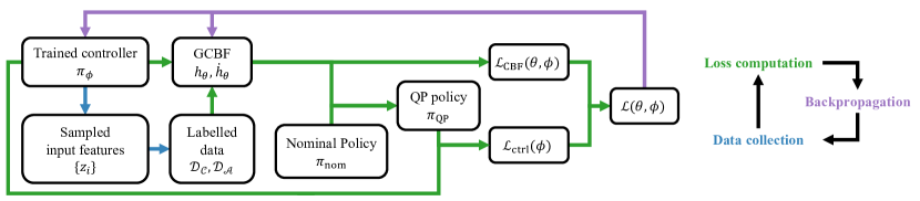
Figure 3: GCBF+ training architecture: The sampled input features are labeled as safe control invariant $\mathcal{D}_{\mathcal{C}}$ and unsafe $\mathcal{D}_{\mathcal{A}}$ using the previous step learned control policy $\pi_{\phi}$ for training. A nominal control policy $\pi_{\mathrm{nom}}$ for goal reaching is used in a CBF-QP with the previously learned GCBF $h_{\theta}$ to generate $\pi_{\mathrm{QP}}$. Finally, the QP policy along with the CBF conditions are used to define the loss $\mathcal{L}$.

IV GCBF+: framework for learning GCBF and distributed control policy

IV-A Neural GCBF and distributed control policy

Drawing on the graph representation of arbitrary sized MAS introduced in Section III-A, we apply GNNs to learn a GCBF $h_{\theta}$ and distributed control policy $\pi_{\phi}$ for parameters $\theta,\phi$. We transform the MAS graph into input features to be used as the GNN input by constructing node features and edge features corresponding to the nodes and edges of the graph $G$. To learn a goal-conditioned control policy that can reach different goal positions, we introduce a goal node and an edge between each agent and their goal in the input features.

Node features and edge features The node features $v_{i}\in\mathbb{R}^{\rho_{v}}$ encode information specific to each node. In this work, we take $\rho_{v}=3$ and use the node features $v_{i}$ to one-hot encode the type of the node as either an agent node, goal node or LiDAR ray hitting point node. The edge features $e_{ij}\in\mathbb{R}^{\rho_{e}}$, where $\rho_{e}>0$ is the edge dimension, are defined as the information shared from node $j$ to agent $i$, which depends on the states of the nodes $i$ and $j$. Since the safety objective depends on the relative positions, one component of the edge features is the relative position $p_{ij}=p_{j}-p_{i}$. The rest of the edge features can be chosen depending on the underlying system dynamics, e.g., relative velocities for double integrator dynamics.

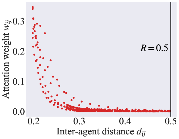
Figure 4: Satisfaction of Assumption 1 in practice: The attention weights $w_{ij}$ in (18) are plotted against inter-agent distances $d_{ij}$ for sensing radius $R=0.5$ from multiple trajectories. The weight $w_{ij}$ approaches $0$ as the inter-agent distance $d_{ij}$ approaches $R$ without explicit supervision, showing that GCBF+ automatically learns to satisfy 1 via the approach outlined in 3.

GNN structure Thanks to the ability of GNN to take variable-sized inputs, we do not need to add padding nor truncate the input of the GCBF into a fixed-sized vector when $\big{\lvert}\tilde{\mathcal{N}}_{i}\big{\rvert}\not=M$. We define the input of $h_{\theta}$ to be input features $z_{i}=\left[z_{i1}^{\top},z_{i2}^{\top},...,z_{i\lvert\tilde{\mathcal{N}}_{i}\rvert}^{\top}\right]^{\top}$, where $z_{ij}=\left[v_{i},v_{j},e_{ij}\right]^{\top}$. In the GNN used for GCBF, we first encode each $z_{ij}$ to the feature space via an MLP $\psi_{\theta_{1}}$ to obtain $q_{ij}=\psi_{\theta_{1}}(z_{ij})$. Next, we use graph attention [63] to aggregate the features of the neighbors of each node, i.e.,

$$q_{i}=\sum_{j\in\tilde{\mathcal{N}}_{i}}\underbrace{\operatorname{softmax}\big{(}\psi_{\theta_{2}}(q_{ij})\big{)}}_{w_{ij}}\,\psi_{\theta_{3}}(q_{ij}),$$ (18)

where $\psi_{\theta_{2}}$ and $\psi_{\theta_{3}}$ are two NNs parameterized by $\theta_{2}$ and $\theta_{3}$. $\psi_{\theta_{2}}$ is often called “gate” NN in literature [66], and the resulting attention weights $w_{ij}\in[0,1]$ (with $\sum\limits_{j\in\mathcal{N}_{i}}w_{ij}=1$) encode how important the sender node $j$ is to agent $i$. Note that applying attention in the GNNs is crucial for satisfying 1. We observe that 1 is satisfied in our experiments since the attention weights and their derivatives go to $0$ as the inter-agent distance goes to $R$ without any additional supervision (see 3 and Figure 4). The aggregated information $q_{i}$ in (18) is then passed through another MLP $\psi_{\theta_{4}}$ to obtain the output value $h_{i}=\psi_{\theta_{4}}(q_{i})$ of the GCBF for each agent. We use the same GNN structure for the control policy $\pi_{\phi}$. Since the input features $z_{i}$ for agent $i$ only depend on the neighbors $\tilde{\mathcal{N}}_{i}$, the $\pi_{\phi}$ is distributed unlike (17).

IV-B GCBF+ loss functions

We train the GCBF $h_{\theta}$ and the distributed controller $\pi_{\phi}$ by minimizing the sum of the CBF loss $\mathcal{L}_{\mathrm{CBF}}(\theta,\phi)$ and the control loss $\mathcal{L}_{\mathrm{ctrl}}(\phi)$:

$$\mathcal{L}(\theta,\phi)=\mathcal{L}_{\mathrm{CBF}}(\theta,\phi)+\mathcal{L}_{\mathrm{ctrl}}(\phi).$$ (19)

The CBF loss $\mathcal{L}_{\mathrm{CBF}}(\theta,\phi)$ and the control loss $\mathcal{L}_{\mathrm{ctrl}}(\phi)$ are defined as sums over each agent as

$$\mathcal{L}_{\mathrm{CBF}}(\theta,\phi)\coloneqq\sum_{i\in V_{a}}\mathcal{L}_{\mathrm{CBF},i}(\theta,\phi),$$ (20a)

$$\mathcal{L}_{\mathrm{ctrl}}(\phi)\coloneqq\sum_{i\in V_{a}}\mathcal{L}_{\mathrm{ctrl},i}(\phi).$$ (20b)

Denote by $\mathcal{D}_{\mathcal{C},i},\mathcal{D}_{\mathcal{A},i}$ the set consisting of labeled input features in the safe control invariant region and unsafe region, respectively. The CBF loss $\mathcal{L}_{\mathrm{CBF},i}$ penalizes violations of the GCBF condition (5) and the (sufficient) safety requirement that the $0$-superlevel set $\mathcal{C}_{N,i}$ is a subset of $S_{N,i}$ (see 5):

$$\mathcal{L}_{\mathrm{CBF},i}(\theta,\phi)\coloneqq\eta_{\mathrm{deriv}}\sum_{z_{i}}\left[\gamma-\dot{h}_{\theta}(z_{i})-\alpha(h_{\theta}(z_{i}))\right]^{+}\\ +\sum_{z_{i}\in\mathcal{D}_{\mathcal{C},i}}\left[\gamma-h_{\theta}(z_{i})\right]^{+}+\sum_{z_{i}\in\mathcal{D}_{\mathcal{A},i}}\left[\gamma+h_{\theta}(z_{i})\right]^{+},$$ (21)

where $\gamma>0$ is a hyper-parameter to encourage strict inequalities and $\eta_{\mathrm{deriv}}>0$ weighs the satisfaction of the GCBF condition (5). We use a linear class-$\mathcal{K}$ function $\alpha(h)=\bar{\alpha}h$ for a constant $\bar{\alpha}>0$. From hereon after, we abuse the notation and use $\alpha$ to refer to $\bar{\alpha}$. The control loss $\mathcal{L}_{\mathrm{ctrl},i}$ encourages the learned controller $\pi_{\phi}$ to remain close to the QP controller $\pi_{\mathrm{QP}}$ (the solution to the QP problem (17) with $h$ being the learned GCBF $h_{\theta}$ in the previous learning step), which in turn is the closest control to $\pi_{\mathrm{nom}}$ that maintains safety:

$$\mathcal{L}_{\mathrm{ctrl},i}(\phi)\coloneqq\eta_{\mathrm{ctrl}}\left\|\pi_{\phi}(z_{i})-\pi_{\mathrm{QP},i}(\bar{x})\right\|,$$ (22)

where $\eta_{\mathrm{ctrl}}$ is the control loss weight and $\pi_{\mathrm{QP},i}(\bar{x})\in\mathcal{U}$ is the $i$-th component of $\pi_{\mathrm{QP}}(\bar{x})$.

One of the challenges of evaluating the loss function $\mathcal{L}$ is computing the time derivative $\dot{h}_{\theta}$. Similar to [56], we estimate $\dot{h}_{\theta}$ by $\left(h_{\theta}(z_{i}(t_{k+1}))-h_{\theta}(z_{i}(t_{k}))\right)/\delta t$, where $\delta t=t_{k+1}-t_{k}$ is the simulation timestep. Estimating $\dot{h}_{\theta}$ may be problematic if the set of neighbors $\tilde{\mathcal{N}}_{i}$ changes between $t_{k}$ and $t_{k+1}$. However, the learned attention weights satisfy 1 as noted previously in Section IV-A. Consequently, 2 implies that $h$ is continuously differentiable, and our estimate of $\dot{h}_{\theta}$ is well behaved. Note that $\dot{h}_{\theta}$ includes the inputs from agent $i$ as well as the neighbor agents $j\in\mathcal{N}_{i}$. Therefore, during training, when we use gradient descent and backpropagate $\mathcal{L}_{i}(\theta,\phi)$, the gradients are passed to not only the controller of agent $i$ but also the controllers of all neighbors in $\tilde{\mathcal{N}}_{i}$. More details on the training process are provided in Section V-A. The training architecture is summarized in Figure 3.

Remark 6.

Benefits of the new loss function   In the prior works  [28, 40], the nominal policy $\pi_{\mathrm{nom}}$ is used instead of $\pi_{\mathrm{QP}}$ in the control loss term. As a result, these approaches suffer from a trade-off between collision avoidance and goal-reaching and often learn a sub-optimal policy that compromises safety for liveness, or liveness for safety. In contrast, our proposed formulation allows the loss to converge to zero, and thus, does not have this trade-off.

Figure 5 plots the closed-loop trajectories of an agent in the presence of an obstacle in its path toward its goal under learned policies with $\pi_{\mathrm{nom}}$ and $\pi_{\mathrm{QP}}$ in the control loss. When $\pi_{\mathrm{nom}}$ is used, for small values of $\eta_{\mathrm{ctrl}}$, the learned controller over-prioritizes safety leading to conservative behavior as illustrated in the top left plot of Figure 5. On the other hand, for large values of $\eta_{\mathrm{ctrl}}$, the learned policy over-prioritizes goal reaching, leading to unsafe behaviors (as in the top right plot). Using an optimal value of $\eta_{\mathrm{ctrl}}$, it is possible to get a desirable behavior as in the top middle plot. In contrast, when $\pi_{\mathrm{QP}}$ is used in the control loss, the goal-reaching and the safety losses do not compete with each other and it is possible to get a desirable behavior without extensive hyper-parameter tuning as can be seen in the bottom plots in Figure 5. Note that when $\pi_{\mathrm{nom}}$ is used, even with the optimal value of $\eta_{\mathrm{ctrl}}$, the learned input (shown with black arrows) does not align with the nominal input (shown with orange arrows). As a result, the total loss may not converge to zero in such formulations unless the nominal policy is also safe. On the other hand, when $\pi_{\mathrm{QP}}$ is used, the two control inputs have much more similar values, which allows for the total loss to converge to $0$.

IV-C Data collection and labeling

The training data $\{z_{i}\}$ is collected over multiple scenarios and the loss is calculated by evaluating the CBF conditions on each sample point. We use an on-policy strategy to collect data by periodically executing the learned controller $\pi_{\phi}$, which helps align the train and test distributions.

When labeling the training data as $\mathcal{D}_{\mathcal{C},i}$ or $\mathcal{D}_{\mathcal{A},i}$, it is important to note that an input feature $z_{i}$ that is not in a collision may be unable to prevent an inevitable collision in the future under actuation limits. For example, under acceleration limits, an agent that is moving too fast may not have enough time to stop, resulting in an inevitable collision. Therefore, we cannot naïvely label all the input features as $\mathcal{D}_{\mathcal{C},i}$ if they are not in any collision at the current time step unless there exists a control policy that can keep them safe in the future. However, as noted in [67, 68, 69, 45, 70], computing an infinite horizon control invariant set for high dimensional nonlinear systems is computationally challenging, and often, various approximations are used for such computations. In this work, we use a finite-time reachable set of the learned policy as an approximation. At any given learning step, given a graph $G$, and the corresponding input features $z_{i},i\in V_{a}$, we use the learned policy from the previous iteration to propagate the system trajectories for $T$ timesteps. If the entire trajectory remains in the safe set $S_{N,i}$ for agent $i$, then $z_{i}$ is added to the set $\mathcal{D}_{\mathcal{C},i}$. If there exist collisions in $z_{i}$, it is added to the set $\mathcal{D}_{\mathcal{A},i}$. Otherwise, it is left unlabeled. As $T\to\infty$, this recovers the infinite horizon control invariant set, but is not tractable to compute. Instead, we choose a large but finite value of $T$ and find it to work well enough in practice.

Remark 7.

Importance of control invariant labels   Note that GCBFv0  [28] does not use the concept of the safe control invariant set during training. Instead, similar to prior works  [42, 71, 40], the learned CBF is enforced to be positive on the entire safe set $\mathcal{S}_{N,i}$, even for states that are not control invariant. Prior works attempt to alleviate these issues by introducing a margin between the safe and unsafe sets, but this is unlikely to result in a control-invariant set for high relative degree dynamics. As noted in [45], if the safe set $\mathcal{S}_{N,i}$ is not control-invariant, then no valid CBF exists that is positive on $\mathcal{S}_{N,i}$. We later investigate the importance of the quality of the control invariant labels (as controlled by $T$) in Section VI-C and find that poor approximations of the control invariant set $\mathcal{C}_{N,i}$ via small values of $T$ leads to large drops in the safety rate. This provides some insight to the performance improvements of GCBF+ over GCBFv0.

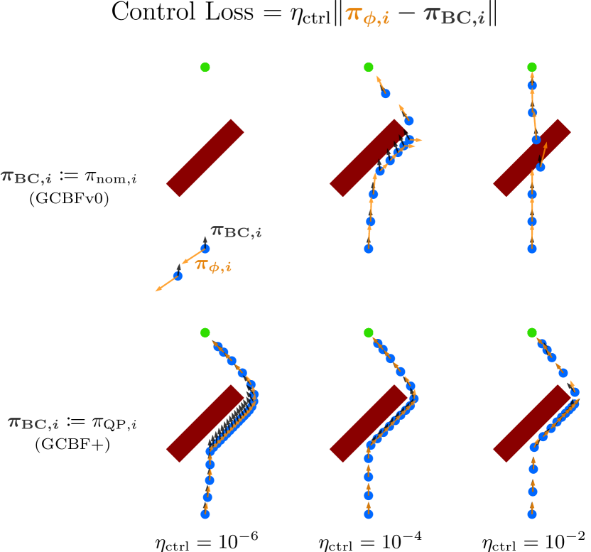
Figure 5: Comparison of the choice of control loss: The learned policy $\boldsymbol{{\color[rgb]{0.90234375,0.515625,0.04296875}\pi_{\phi}}}$ is sensitive to the choice of $\eta_{\mathrm{ctrl}}$ when using $\pi_{\mathrm{nom}}$ as in GCBFv0 [28] (top) since a learned policy $\boldsymbol{{\color[rgb]{0.90234375,0.515625,0.04296875}\pi_{\phi}}}$ that is close to $\pi_{\mathrm{nom}}$ may be unsafe and not satisfy the GCBF conditions (5). Consequently, choosing $\eta_{\mathrm{ctrl}}$, which controls the relative weight between $\mathcal{L}_{\mathrm{CBF}}$ and $\mathcal{L}_{{ctrl}}$, becomes a balancing act of staying close to $\pi_{\mathrm{nom}}$ while remaining safe. In contrast, by definition of $\pi_{\mathrm{QP}}$ (17), the control $\boldsymbol{{\color[rgb]{0.90234375,0.515625,0.04296875}\pi_{\phi}}}$ is already safe. Hence, the safety of $\boldsymbol{{\color[rgb]{0.90234375,0.515625,0.04296875}\pi_{\phi}}}$ is not sensitive to $\eta_{\mathrm{ctrl}}$ when using $\pi_{\mathrm{QP}}$ for the control loss, as in GCBF+.

V Experiments: implementation details

In this section, we introduce the details of the experiments, including the implementation details of GCBF+ and the baseline algorithms, and the details of each environment.

Environments  We conduct experiments on five different environments consisting of three 2D environments (SingleIntegrator, DoubleIntegrator, DubinsCar) and two 3D environments (LinearDrone, CrazyflieDrone). See Appendix C for details. The parameters are $R=0.5,r=0.05$ in all environments. The total time steps for each experiment is $4096$.

Evaluation criteria  We use safety rate, reaching rate, and success rate as the evaluation criteria for the performance of a chosen algorithm. The safety rate is defined as the ratio of agents not colliding with either obstacles or other agents during the experiment period over all agents. The goal reaching rate, or simply, the reaching rate, is defined as the ratio of agents reaching their goal location by the end of the experiment period. The success rate is defined as the ratio of agents that are both safe and goal-reaching. We note that the safety metric in [56] is slightly misleading as they measure the portion of collision-free states for safety rate. For each environment, we evaluate the performance over $32$ instances of randomly chosen initial and goal locations for $3$ policies trained with different random seeds. We report the mean rates and their standard deviations for the $32$ instances for each of the $3$ policies (i.e., average performance over $96$ experiments).

V-A Implementation details

Our learning framework contains two neural network models: the GCBF $h_{\theta}$ and the controller $\pi_{\phi}$. The size of the MLP layers in $h_{\theta}$ and $\pi_{\phi}$ are shown in Table I. To make the training easier, we define $\pi_{\phi}$ = $\pi^{\mathrm{NN}}_{\phi}+\pi_{\mathrm{nom}}$, where $\pi^{\mathrm{NN}}_{\phi}$ is the NN controller and $\pi_{\mathrm{nom}}$ is the nominal controller, so that $\pi^{\mathrm{NN}}_{\phi}$ only needs to learn the deviation from $\pi_{\mathrm{nom}}$.

TABLE I: Size of hidden layers and output layers of the MLP used in the GNN.

MLP	Hidden layer size	Output layer size
$\psi_{\theta_{1}}$	$256\times 256$	$128$
$\psi_{\theta_{2}}$	$128\times 128$	$1$
$\psi_{\theta_{3}}$	$256\times 256$	$128$
$\psi_{\theta_{4}}$	$256\times 256$	$1$ for $h_{\theta}$ and $m$ for $\pi_{\phi}$

We use Adam [72] to optimize the NNs for $1000$ steps in training. The training time is around $3$ hours on a 13th Gen Intel(R) Core(TM) i7-13700KF CPU @ $3400\mathrm{MHz}$ and an NVIDIA RTX 3090 GPU. We choose the hyper-parameters in the loss $\mathcal{L}$ following Table II, where "lr cbf" and "lr policy" denote the learning rate for the GCBF $h_{\theta}$ and control policy $\pi_{\phi}$, respectively. We set $\alpha=1.0$, $\gamma=0.02$, and $\eta_{\mathrm{deriv}}=0.2$ for all the environments.

TABLE II: Hyper-parameters used in our training

Environment	$T$	$\eta_{\mathrm{ctrl}}$	lr policy	lr GCBF
SingleIntegrator	$1$	$10^{-4}$	$10^{-5}$	$10^{-5}$
DoubleIntegrator	$32$	$10^{-4}$	$10^{-5}$	$10^{-5}$
DubinsCar	$32$	$10^{-5}$	$3\times 10^{-5}$	$3\times 10^{-5}$
LinearDrone	$32$	$10^{-3}$	$10^{-5}$	$10^{-5}$
CrazyflieDrone	$32$	$3\times 10^{-5}$	$10^{-5}$	$10^{-4}$

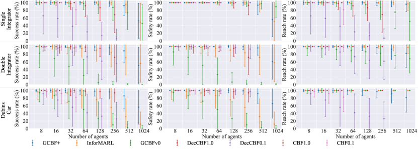
(a) 2D environments

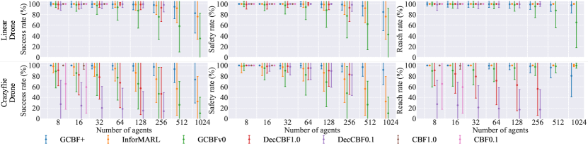
(b) 3D environments

Figure 6: Success (left), safety (middle), and reach (right) rates for an increasing number of agents for fixed area width $l$.

V-B Baseline methods

We compare the proposed method (GCBF+) with GCBFv0 [28], InforMARL [29], and centralized and distributed variants of hand-crafted CBF-QPs [23]. We use a modified version of the GCBFv0 introduced in [28] where we remove the online policy refinement step since it requires multiple rounds of inter-agent communications to exchange control inputs during execution and does not work in the presence of actuation limits.

The InforMARL algorithm is a variant of MAPPO [16] that uses a GNN architecture for the actor and critic networks. We use a reward function that consists of three terms. First, we penalize deviations from the nominal controller, i.e.,

$$R_{\textrm{nom},i}\coloneqq-\frac{1}{2}\left\lVert u_{i}-u_{i}^{\mathrm{nom}}\right\rVert^{2}.$$ (23)

To improve performance, we use a sparse reward term for reaching the goal, i.e.,

$$R_{\textrm{goal},i}\coloneqq\begin{dcases}1.0,&\left\lVert p_{i}-p^{g}_{i}\right\rVert\leq 2r\\ 0&\textrm{otherwise}\end{dcases}$$ (24)

Safety is incorporated by adding the following term to the reward function to penalize collisions, similar to [73, 74]:

$$R_{\textrm{col},i} \coloneqq\max_{j}R_{\textrm{col},ij},$$ (25)

$$R_{\textrm{col},ij} \coloneqq\begin{dcases}-1&\left\lVert p_{i}-p_{j}\right\rVert<2r,\\ \frac{\left\lVert p_{i}-p_{j}\right\rVert}{2r}-2&2r\leq\left\lVert p_{i}-p_{j}\right\rVert\leq 4r,\\ 0&4r<\left\lVert p_{i}-p_{j}\right\rVert,\end{dcases}$$ (26)

where the $\max$ over $j\in\tilde{\mathcal{N}}_{i}$. The final reward function for each agent $i$ is a sum of the above three terms weighted by $\lambda_{\text{nom}}$, $\lambda_{\text{goal}}$ and $\lambda_{\text{col}}>0$.

$$R_{i}\coloneqq\lambda_{\text{nom}}R_{\text{nom},i}+\lambda_{\text{goal}}R_{\text{goal},i}+\lambda_{\text{col}}R_{\text{col},i}$$ (27)

For the hand-crafted CBF-QPs, we use a pairwise CBF between each pair of agents $(i.j)$, defined as the following higher-order CBF [75, 76]

$$h_{0} =\sum_{l\in\mathbb{P}}(p_{i}^{l}-p_{j}^{l})^{2}-(2r)^{2}$$ (28)

$$h =\dot{h}_{0}+\alpha_{0}h_{0},$$ (29)

where $\mathbb{P}=\{x,y\}$ for 2D environments and $\mathbb{P}=\{x,y,z\}$ for 3D environments, $\alpha_{0}\in\mathbb{R}_{+}$ is a constant and $r$ is the radius of the agent. We consider two CBF-QP frameworks [23]:

• Centralized CBF: In this framework, inputs of all the agents are solved together by setting up a centralized QP containing CBF constraints of all the agents. In this case, the CBF condition is

  $$\dot{h}+\alpha h\geq 0.$$ (30)

• Decentralized CBF: In this framework, each agent computes its control input but the CBF condition is shared between the neighbors as in [23]. Let $\dot{x}_{ij}=f_{ij}(x_{ij})+g_{ij,i}(x_{ij})u_{i}+g_{ij,j}(x_{ij})u_{j}$ denote the combined dynamics of the pair $(i,j)$ where $f_{ij},g_{ij,i},g_{ij,j}$ can be obtained from combining the agent dynamics. Then, the constraint used in the agent $i$’s QP is:

  $$\frac{\partial h}{\partial x_{ij}}g_{ij,i}(x_{ij})u_{i}\geq-\frac{1}{2}\left(\alpha h(x_{ij})+\frac{\partial h}{\partial x_{ij}}{f_{ij}}(x_{ij})\right),$$ (31)

  while that in agent $j$’s QP is:

  $$\frac{\partial h}{\partial x_{ij}}g_{ij,j}(x_{ij})u_{j}\geq-\frac{1}{2}\left(\alpha h(x_{ij})+\frac{\partial h}{\partial x_{ij}}{f_{ij}}(x_{ij})\right),$$ (32)

  so that the sum of the constraints (31) and (32) recovers the CBF condition (30).

For both centralized and decentralized approaches, we design two baselines with $\alpha=1.0$ and $\alpha=0.1$, respectively. The resulting $4$ baselines are named CBF1.0, CBF0.1, DecCBF1.0, and DecCBF0.1, respectively.

VI Numerical experiments: results

We first conduct experiments in simulation to examine the scalability, generalizability and effectiveness of the proposed method. In all experiments, the initial position of the agents and goals are uniformly sampled from the set $\mathbb{P}_{0}=[0,l]^{\mathfrak{n}}$ for an area width $l>0$ which we specify for each environment. The density of agents can be approximately computed as $N/l^{\mathfrak{n}}$. Hence, a smaller value of $l$ results in a higher density of agents and thus is more challenging to prevent collisions.

In all experiments, we train the algorithms on an environment with $8$ agents and $8$ obstacles with $l=4$ for 2D and $l=2$ for 3D environments.

VI-A Performance under increasing number of agents

We first perform experiments in an obstacle-free setting where we test the algorithms for a fixed $l$ but increase the number of agents $N$ from $8$ to $1024$. This tests the ability of each algorithm to maintain safety as the density of agents and goals in the environment increases by over $100$-fold. We use $l=8$ for SingleIntegrator and DoubleIntegrator environments, $l=16$ for the DubinsCar environment, and $l=4$ for both the 3D environments and show the resulting success rate, safety rate and reach rate in Figure 6.

Centralized methods do not scale with increasing number of agents. As expected, the centralized methods (i.e., CBF1.0 and CBF0.1) require increasing amounts of computation time as the number of agents increases. Consequently, we were unable to test CBF1.0 and CBF0.1 for more than $32$ agents in all environments due to exceeding computation limits.

Decentralized CBF are overly conservative. The decentralized CBF-QP method with $\alpha=0.1$ has comparable safety performance to GCBF+. However, it is much more conservative than GCBF+ and compromises on its goal-reaching ability, as evident from the low reach rates across all environments. For larger values of $\alpha$, the decentralized CBF-QP method fails to maintain a high safety rate as the controls become saturated by the control limit. Although the decentralized CBF can be scaled to a large number of agents assuming that each agent can perform computation for its control input locally, in our experiments, we simulate the decentralized controller on one computer node and hence are constrained by the memory and computation limits of the computer. Thus, we could not perform experiments for more than $256$ agents due to this constraint. However, the downward trend of the reaching rate illustrates that the decentralized CBF-QP method becomes more conservative as the environment gets denser.

GCBFv0 struggles with safety for dynamics with high relative degrees. While GCBFv0 performs comparably on the SingleIntegrator environment, the performance deteriorates drastically on all other dynamics. This is because GCBFv0 relies on an accurate hand-crafted safe control invariant set during training, which is difficult to estimate in the presence of control limits for dynamics with high relative degrees. The safe control invariant set is easy to estimate for relative degree $1$ environments such as SingleIntegrator, where it can be taken as the complement of the unsafe set. However, for high relative degree dynamics with control limits, the naive estimation method used by GCBFv0 breaks down, causing the safety rate and thus success rate to drop significantly. Another potential reason for the poor safety of GCBFv0 is that it uses $\pi_{\mathrm{nom}}$ in the control loss, which forces a trade-off between safety and goal-reaching (see 6).

GCBF+ performs well on nonlinear dynamics. We observe that all methods have lower success rates on environments that have nonlinear dynamics (DubinsCar, CrazyflieDrone) compared to ones with linear dynamics (SingleIntegrator, DoubleIntegrator, LinearDrone). The performance gap between GCBF+ and other methods is more clear on these challenging environments. On the DubinsCar environment, GCBF+ achieves a $44\%$ higher (compared to InforMARL) and $55\%$ higher (compared to GCBFv0) success rate. On the CrazyflieDrone environment, GCBF+ achieves a $45\%$ higher (compared to InforMARL) and $65\%$ higher (compared to GCBFv0) success rate. Hence, GCBF+ generalizes better than the baseline algorithms, particularly for environments with nonlinear dynamics.

GCBF+ reach rate declines faster than InforMARL While the safety rate for GCBF+ is the best among the baselines for denser environments, its reach rate declines as the number of agents increases, while the reach rate for InforMARL stays consistently near $100\%$ in all environments. The main reason for this decline is the fact that the GCBF+ algorithm focuses on safety and delegates the liveness (i.e., goal-reaching) requirements to the nominal controller which is unable to resolve deadlocks. Hence, one potential reason for the lower reach rates of GCBF+ as the density increases is that the learned controller is unable to resolve deadlocks that occur more frequently with increasing density. On the other hand, InforMARL has a sparse reward term for reaching the goal (24) and hence, it is incentivized to learn a controller that can resolve deadlocks at the cost of temporarily deviating from the nominal controller and sacrificing safety, which is evident from the significant drop in the safety rate for InforMARL.

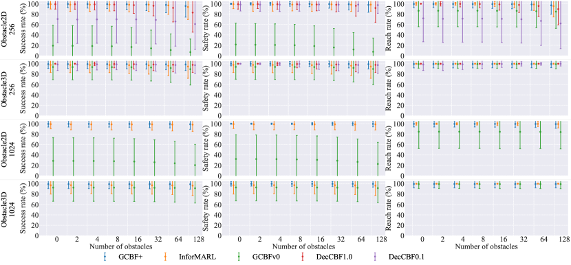
Figure 7: Obstacle environment performance: Success (left), safety (middle), and reach (right) rates for the obstacle environment in one 2D and one 3D environment, namely, DoubleIntegrator and LinearDrone environments. In these experiments, the number of agents as well as the area size are kept constant while the number of obstacles are increased. The first set of experiments is conducted on 256 agents with all the baselines. The second set of experiments is conducted with 1024 agents with only GCBF and InforMARL for comparison since we were unable to simulate hand-crafted CBF-QPs for more than 256 agents due to computational limits.

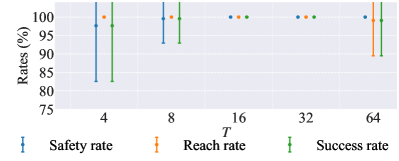
Figure 8: Left: Sensitivity of GCBF+ to the CBF class$-\mathcal{K}$ function parameter $\alpha$. Right: Sensitivity of GCBF+ to prediction horizon $T$ for computation of the control invariant set $\mathcal{S}_{c,i}$.

VI-B Performance under increasing number of obstacles

In the next set of simulation experiments, we fix the number of agents $N$ and the area width $l$ and vary the number of obstacles present from $0$ to $128$. For the 2D DoubleIntegrator environment, we consider $(N=256,l=16)$ and $(N=1024,l=32)$, where the obstacles are cuboids with side lengths uniformly sampled from $[0.1,0.5]$ and each agent generates $32$ equally spaced LiDAR rays to detect obstacles. For the 3D LinearDrone environment, we consider $(N=256,l=8)$ and $(N=1024,l=12)$, where the obstacles are spheres with radius uniformly sampled from $[0.15,0.3]$ and each agent generates $130$ equally spaced LiDAR rays to detect obstacles.

The success rate, safety rate and reach rate for all cases is shown in Figure 7. Overall, we observe similar trends as the previous experiment in Section VI-A. In all environments, GCBF+ has the highest success rates compared with the baselines. Trained with just $8$ agents and $8$ obstacles, GCBF+ can achieve a $>98\%$ success rate with $256$ (and $1024$) agents and $128$ obstacles. InforMARL performs well but is behind GCBF+. Other baselines have much lower success rates compared with GCBF+ and InforMARL. GCBFv0 does not perform well since it does not account for control limits. The decentralized CBFs perform poorly in the 2D environment due to their conservatism and in the 3D environment due to saturation from the control limits.

VI-C Sensitivity to hyper-parameters

We next perform a sensitivity analysis of our proposed method on the DoubleIntegrator environment to investigate the effect of two hyper-parameters: $\alpha$ and $T$. The $\alpha$ parameter is used to define the CBF derivative condition (21), while $T$ is used to label safe control invariant data and unsafe data (see Section IV-C). We plot the success, reach, and safety rates while varying $\alpha$ from $10^{-2}$ to $10^{2}$ in the left plot in Figure 8. The results showed that using $\alpha=10^{-2}$ led to a drop in the reach rate, while using $\alpha=10^{2}$ led to a drop in the safety rate. This behavior can be attributed to the fact that for very small values of $\alpha$, the CBF condition becomes overly conservative, resulting in poor goal-reaching. For very large values of $\alpha$, safety can be compromised as the CBF condition allows the system to move towards the unsafe set at a faster rate. This, along with the fact that the control inputs are constrained, may lead to a violation of safety.

Note that for a relatively large range of the parameter $\alpha$, namely, $\alpha\in[0.1,10]$, the performance of GCBF+ does not change much. This implies that GCBF+ is robust to a large range of $\alpha$.

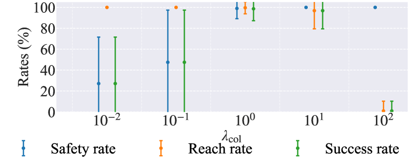
Figure 9: Sensitivity of InforMARL to the weight $\lambda_{\mathrm{col}}$ in (27).

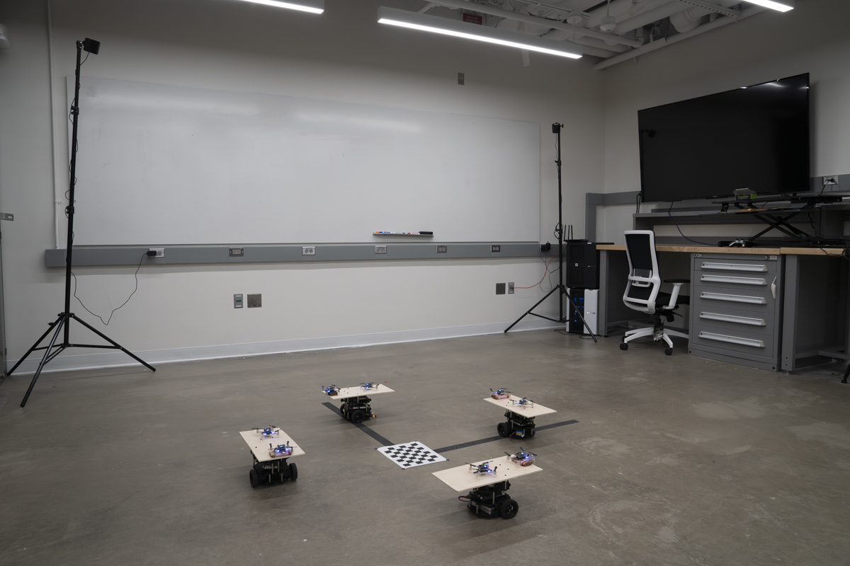
(a)

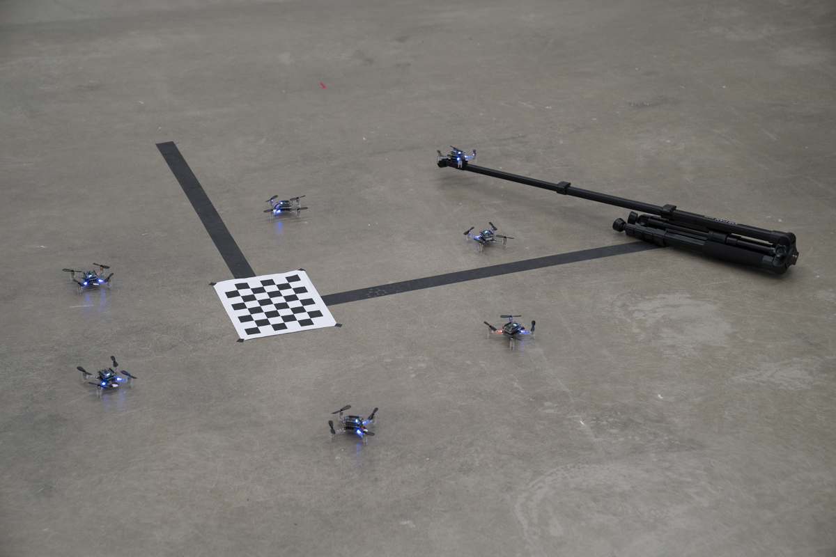
(b)

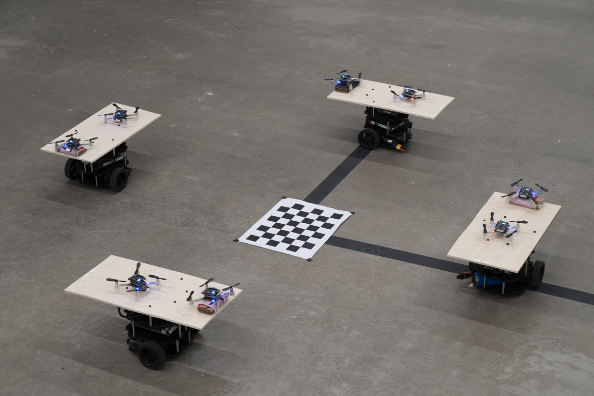
(c)

Figure 10: Hardware experiment setup: (a) The overall experimental setup with ground robots, CF drones and the motion capture system. (b) Setup for the position exchange with a moving obstacle. The intruder drone or the moving obstacle is mounted on a tripod to be moved around randomly. (c) Setup for tracking and landing on a moving platform.

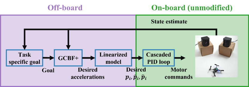
Figure 11: Hardware Control Architecture for Crazyflies

The right plot in Figure 8 analyzes the performance of GCBF+ for a varying prediction horizons $T\in[4,64]$ for labeling the data to be safe control invariant or unsafe for training. For a very small horizon $T=4$, the safety rate drops as the resulting approximation of the safe control invariant set is poor for such a small horizon. For a very large horizon $T=64$, the algorithm becomes too conservative, requiring longer training times to converge. For the chosen fixed number of training steps, we observe that the resulting controller, while maintaining $100\%$ safety, achieves $98\%$ goal-reaching rate. However, as can be seen from the plots, GCBF+ is mildly sensitive to this parameter only at its extreme values, and almost insensitive in the nominal range $T\in[8,32]$.

As InforMARL has the best performance among baselines, we analyze its sensitivity as well. Figure 9 analyzes the sensitivity of the performance of InforMARL to the weight $\lambda_{\mathrm{col}}$ that dictates the penalty for collision in the RL reward function 27. It can be observed that for a relatively small range of $\lambda_{\mathrm{col}}\in[1,10]$, InforMARL achieves high performance. For smaller values of this weight, the RL-based method over-prioritizes goal-reaching, compromising on safety, and for larger values of this weight, the goal-reaching performance is poor due to over-prioritization of the system safety.

These experiments illustrate that the proposed algorithm GCBF+ is not as sensitive to its crucial hyper-parameters as InforMARL, and hence, does not require fine-tuning of such parameters to obtain desirable results.

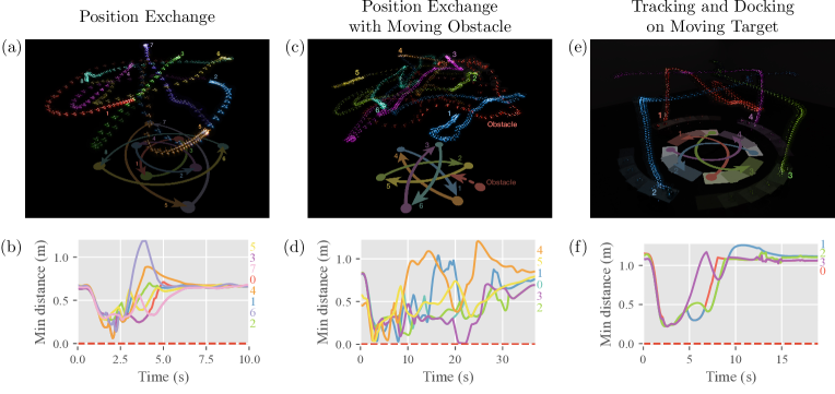
Figure 12: Hardware Experiment Results: (a,c,e) Time-lapse illustration of a Crazyflie swarm controlled via GCBF+. (b,d,f) The associated minimum distances for each agent to other agents and obstacles.

VII Hardware experiments

We conduct hardware experiments on a swarm of Crazyflie (CF) 2.1 platform to illustrate the applicability of the proposed method on real robotic systems. We conduct three sets of experiments as discussed below. The hardware setup is illustrated in Figure 10. We use a set of eight CF drones for the experiments. To communicate with the CFs, two Crazyradios are used so that four CFs are allocated on each of the Crazyradios. Localization is performed using the Lighthouse localization system. Four SteamVR Base Station 2.0 are mounted on tripods and placed on the corners of the flight area.

VII-A Control architecture

An overview of the hardware control architecture is presented in Figure 11. Computation is split into onboard, i.e., on the CF micro-controller unit (MCU), and off-board, i.e., a laptop connected to the CFs over Crazyradio.

Offboard computation happens on a laptop connected to the CFs over Crazyradios. To communicate with the Crazyflies, we use the crazyswarm2 ROS2 package. This allows for receiving full state estimates from and sending control commands to the CFs. We use a single ROS2 node to perform the off-board computations at 50 Hz.

Task Specific Logic To begin, the state estimates are used to compute a task-specific goal position for each of the CFs. For the swapping tasks, the goals are static and do not change. For the docking task, we take the location of the Turtlebots to be the goal position.

GCBF+ Controller The goal positions and the state estimates (position and velocities) are next used to compute target accelerations for each CF using the GCBF+ controller. This GCBF+ controller is trained using double integrator dynamics.

Ideal Dynamics Model To track the computed desired accelerations from GCBF+, we make use of the cmd_full_state interface in crazyswarm2. However, cmd_full_state requires set points for the whole state (i.e., also position and velocity) instead of just accelerations. To resolve this problem, we simulate the ideal dynamics model (i.e., double integrator) used for training GCBF+ and take the resulting future positions and velocities that would result from applying the desired accelerations after some duration $\Delta t$. We used $\Delta t=\mathrm{50ms}$ in our hardware experiments.

We do not modify the onboard computation. The received full state set points are used as set points for a cascaded PID controller, as described in the Crazyflie documentation.

VII-B Experimental results

We conduct the following three sets of hardware experiments.

Position exchange  In this experiment, we arrange the CF drones in a circular configuration with the objective of each drone exchanging position with the diagonally opposite drone. We perform experiments with up to $8$ drones. This is a typical experiment setting used for illustration of the capability of an algorithm to maintain safety where there are many inter-agent interactions. The resulting trajectories of the drones are plotted in Figure 12(a-b). As can be observed from the figure, the CF drones maintain the required safe distance and land safely at their desired location.

Position exchange under moving obstacle  In this experiment, we add a moving obstacle to the setup from the previous experiment. The moving obstacle is moved arbitrarily around the environment by a human subject. The path of the moving obstacle is not known beforehand by the controlled CF drones. Figures 12(c-d) illustrate that safety is maintained at all times.

Tracking and landing on moving target  In this experiment, the CF drones are required to track a moving ground vehicle and land on it. For this experiment, instead of a simple LQR controller, a back-stepping controller is used as a nominal controller that can track a moving target with time-varying acceleration. We use four Turtlebot 3 mobile robots as the moving target, equipped with a platform on its top where a CF drone can land. Initially, one CF drone is placed on each of the Turtlebots. The drones take off and start tracking the diagonally opposite moving target, while the Turtlebots move in a circular trajectory. From Figures 12(e-f), the drones successfully land on the moving targets while maintaining safety with each other in this dynamically changing environment. This illustrates the generalizability of GCBF+ to a variety of control problems.

Experiment videos  The numerical and hardware experiment videos are available at https://mit-realm.github.io/gcbfplus-website/.

VIII Conclusions

In this paper, we introduce a new class of graph control barrier function, termed GCBF, to encode inter-agent and obstacle collision avoidance in a large-scale MAS. We propose GCBF+, a training framework that utilizes GNNs for learning a GCBF candidate and a distributed control policy using only local observations. The proposed framework can also incorporate LiDAR point-cloud observations instead of actual obstacle locations, for real-world applications. Numerical experiments illustrate the efficacy of the proposed framework in achieving high safety rates in dense multi-agent problems and its superiority over the baselines for MAS consisting of nonlinear dynamical agents. Trained on 8 agents, GCBF+ achieves over 80% safety rate in environments with more than 1000 agents, demonstrating its generalizability and scalability. A major advantage of the GCBF+ algorithm is that it does not have a trade-off between safety and performance, as is the case with reinforcement learning (RL)-based methods. Furthermore, hardware experiments demonstrate its applicability to real-world robotic systems.

The proposed work has a few limitations. In the current framework, there is no cooperation among the controlled agents, which leads to conservative behaviors. In certain scenarios, this can also lead to deadlocks resulting in a lower reaching rate, as observed in the numerical experiments as well. We are currently investigating methods of designing a high-level planner that can resolve such deadlocks and lead to improved performance. Similar to other NN-based control policies, the proposed method also suffers from difficulty in providing formal guarantees of correctness. In particular, it is difficult, if not impossible, to verify that the proposed algorithm can always keep the system safe via formal verification of the learned neural networks (see Appendix 1 in [77] on NP-completeness of NN-verification problem). This informs our future line of work on looking into methods of verification of the correctness of the control policy.

Appendix A Proof of the claim in Remark 1

For any $i\in V_{a}$, by definition of $M$ and the continuity of the position of nodes, changes in the neighboring indices $\mathcal{N}_{i}$ can only occur without collision at a distance $R$. To see this, we consider the following three cases.

Case 1: $\left\lvert\tilde{\mathcal{N}}_{i}\right\rvert<M$, i.e., the number of neighbors is less than $M$. In this case, $\mathcal{N}_{i}=\tilde{\mathcal{N}}_{i}$ and hence, a node $j$ is added or removed to $\mathcal{N}_{i}=\tilde{\mathcal{N}}_{i}$ when it enters or leaves the sensing radius $R$.

Case 2: $\left\lvert\tilde{\mathcal{N}}_{i}\right\rvert>M$, i.e., the number of neighbors is more than $M$. In this case, there are more than $M-1$ neighbors of agent $i$ within sensing radius $R$, which, from the definition of $M$, implies that the MAS is unsafe.

Case 3: $\left\lvert\tilde{\mathcal{N}}_{i}\right\rvert=M$, i.e., the number of neighbors is $M$. In this case, if a neighbor is added to $\tilde{\mathcal{N}}_{i}$ without any other agent leaving the set $\tilde{\mathcal{N}}_{i}$, then we obtain Case 2 and the MAS is unsafe. If a node $j$ is removed with no other neighbors added to $\tilde{\mathcal{N}}_{i}$, then this happens when $j$ leaves the sensing radius $R$. Finally, if a node $j$ is removed at the same time that a node $k$ is added without changing the size of $\left\lvert\mathcal{N}_{i}\right\rvert=M$, by the continuity of the position dynamics there exists a time $t$ where both nodes are at the same distance $R$ from $p_{i}$. However, this implies that $\left\lvert\mathcal{N}_{i}\right\rvert=M+1$, and the MAS is unsafe by Case 2.

Consequently, changes in the neighboring indices $\mathcal{N}_{i}$ can only occur without collision at a distance $R$.

Appendix B Proof of Theorem 1

Before we begin the proof, we first state the following lemma, borrowed from [78].

Lemma 1.

Let $h:\mathbb{R}\to\mathbb{R}$ be a continuously differentiable function and $\alpha$ be an extended class-$\mathcal{K}_{\infty}$ function. If $h(0)\geq 0$ and, for some $T\in\mathbb{R}_{+}$,

$$\dot{h}(t)+\alpha(h(t))\geq 0,\quad\forall t\in[0,T],$$ (33)

then $h(T)\geq 0$.

Proof.

The scalar system $v$ with $v(0)=h(0)\geq 0$ and $\dot{v}(t)=-\alpha(v(t))$ admits a unique solution $v(t)$ such that $v(t)\geq 0$ for all $t\geq 0$ [79, Lemma 4.4]. Using the Comparison Lemma [79, Lemma 3.4], it thus follows from $h(0)=v(0)$ and (33) that $h(t)\geq v(t)\geq 0$ for all $t\in[0,T]$. ∎

We are now ready to prove Theorem 1.

Proof.

Consider any $i\in V_{a}$. We first prove that $\bar{x}_{\mathcal{N}_{i}}(t)\in\mathcal{C}_{h}$ for all $t\geq 0$. Define $t_{k}$ for $k\in\mathbb{N}$ with $t_{0}=0$, such that $\mathcal{N}_{i}$ is constant on the time segments $[t_{k},t_{k+1})$ for all $i$ i.e.,

$$t_{k}\coloneqq\inf\{t>t_{k-1}\mid\exists i:\mathcal{N}_{i}(t)\not=\mathcal{N}_{i}(t_{k})\},\quad k\geq 1.$$ (34)

For each such interval $[t_{k},t_{k+1})$, suppose that $h(\bar{x}_{\mathcal{N}_{i}}(t_{k}))\geq 0$. Then, 1 applied to the function $t\mapsto h(\bar{x}_{\mathcal{N}_{i}}(t))$ and (5) implies that

$$h(\bar{x}_{\mathcal{N}_{i}}(t))\geq 0,\quad\forall t\in[t_{k},t_{k+1}).$$ (35)

Since this holds for all $i\in V_{a}$, we obtain that

$$\bar{x}(t_{k})\in\mathcal{C}_{N}\subset\mathcal{S}_{N}\;\implies\;\bar{x}(t)\in\mathcal{C}_{N}\subset\mathcal{S}_{N},\quad\forall t\in[t_{k},t_{k+1}).$$ (36)

For any $i\in V_{a}$ where the neighborhood remains constant, continuity of $h$ implies that $h(t_{k+1})\geq 0$. On the other hand, if the neighborhood $\mathcal{N}_{i}$ changes for some $i$ at $t_{k+1}$, since $\bar{x}$ is safe in the interval $[t_{k},t_{k+1})$, 1 implies that the change must occur when the neighboring node is at least $R_{\mathrm{small}}$ away from $p_{i}$. Then, (35) and (9) implies that $h(t_{k+1})\geq 0$ in this case as well.

Since $h(\bar{x}_{\mathcal{N}_{i}}(0))\geq 0$, applying induction thus gives the result that $h(\bar{x}_{\mathcal{N}_{i}}(t))\geq 0$, and hence $\bar{x}_{\mathcal{N}_{i}}(t)\in\mathcal{C}_{i}$, for all $t\geq 0$. Since this holds for all $i\in V_{a}$, by definition of $\mathcal{C}_{N}$, we have that $\bar{x}\in\mathcal{C}_{N}\subset\mathcal{S}_{N}$ for all $t\geq 0$. ∎

Appendix C Experiment Environments

Here, we provide the details of each experiment environment.

SingleIntegrator   We use single integrator dynamics as the base environment to verify the correctness of the baseline methods and to show the performance of the methods when there are no control input limits. The dynamics is given as $\dot{x}_{i}=v_{i}$, where $x_{i}=[p^{x}_{i},p^{y}_{i}]^{\top}\in\mathbb{R}^{2}$ is the position of the $i$-th agent and $v_{i}=[v^{x}_{i},v^{y}_{i}]^{\top}$ its velocity. In this environment, we use $e_{ij}=x_{j}-x_{i}$ as the edge information. We use the following reward function weights for training InforMARL.

$$\lambda_{\text{nom}}=0.1,\quad\lambda_{\text{goal}}=0.1,\quad\lambda_{\text{col}}=5.0\,.$$ (37)

DoubleIntegrator  We use double integrator dynamics for this environment. The state of agent $i$ is given by $x_{i}=[p^{x}_{i},p^{y}_{i},v^{x}_{i},v^{y}_{i}]^{\top}$, where $[p^{x}_{i},p^{y}_{i}]^{\top}$ is the position of the agent, and $[v^{x}_{i},v^{y}_{i}]^{\top}$ is the velocity. The action of agent $i$ is given by $u_{i}=[a^{x}_{i},a^{y}_{i}]^{\top}$, i.e., the acceleration. The dynamics function is given by:

$$\dot{x}_{i}=\left[v^{x}_{i},v^{y}_{i},a^{x}_{i},a^{y}_{i}\right]^{\top}$$ (38)

The simulation time step is $\delta t=0.03$. In this environment, we use $e_{ij}=x_{j}-x_{i}$ as the edge information. We use the following reward function weights for training InforMARL without obstacles.

$$\lambda_{\text{nom}}=0.1,\quad\lambda_{\text{goal}}=0.1,\quad\lambda_{\text{col}}=2.0\,.$$ (39)

and the following reward function weights with obstacles.

$$\lambda_{\text{nom}}=0.1,\quad\lambda_{\text{goal}}=0.1,\quad\lambda_{\text{col}}=5.0\,.$$ (40)

For the hand-crafted CBFs, we use $\alpha_{0}=10$.

DubinsCar  We use the standard Dubin’s car model in this environment. The state of agent $i$ is given by $x_{i}=[p^{x}_{i},p^{y}_{i},\theta_{i},v_{i}]^{\top}$, where $[p^{x}_{i},p^{y}_{i}]^{\top}$ is the position of the agent, $\theta_{i}$ is the heading, and $v_{i}$ is the speed. The action of agent $i$ is given by $u_{i}=[\omega_{i},a_{i}]^{\top}$ containing angular velocity and longitudinal acceleration. The dynamics function is given by:

$$\dot{x}_{i}=\left[v_{i}\cos(\theta_{i}),v_{i}\sin(\theta_{i}),\omega_{i},a_{i}\right]^{\top}$$ (41)

The simulation time step is $\delta t=0.03$. We use $e_{ij}=e_{j}(x_{j})-e_{i}(x_{i})$ as the edge information, where $e_{i}(x_{i})=[p^{x}_{i},p^{y}_{i},v_{i}\cos(\theta_{i}),v_{i}\sin(\theta_{i})]^{\top}$. We use the following reward function weights for training InforMARL.

$$\lambda_{\text{nom}}=0.1,\quad\lambda_{\text{goal}}=0.1,\quad\lambda_{\text{col}}=1.0\,.$$ (42)

For the hand-crafted CBFs, we use $\alpha_{0}=5$.

LinearDrone  We use a linearized model for drones in our experiments. The state of agent $i$ is given by $x_{i}=[p^{x}_{i},p^{y}_{i},p^{z}_{i},v^{x}_{i},v^{y}_{i},v^{z}_{i}]^{\top}$ where $[p^{x}_{i},p^{y}_{i},p^{z}_{i}]^{\top}$ is the 3D position, and $[v^{x}_{i},v^{y}_{i},v^{z}_{i}]^{\top}$ is the 3D velocity. The control inputs are $u_{i}=[a^{x}_{i},a^{y}_{i},a^{z}_{i}]^{\top}$, and the dynamics function is given by:

$$\dot{x}_{i}=\left[\begin{array}[]{cc}v^{x}_{i}\\ v^{y}_{i}\\ v^{z}_{i}\\ -1.1v^{x}_{i}+1.1a^{x}_{i}\\ -1.1v^{y}_{i}+1.1a^{y}_{i}\\ -6v^{z}_{i}+6a^{z}_{i}\end{array}\right]$$ (43)

The simulation time step is $\delta t=0.03$. We use $e_{ij}=x_{j}-x_{i}$ as the edge information. We use the following reward function weights for training InforMARL.

$$\lambda_{\text{nom}}=1.0,\quad\lambda_{\text{goal}}=0.1,\quad\lambda_{\text{col}}=1.0\,.$$ (44)

For the hand-crafted CBFs, we use $\alpha_{0}=3$.

CrazyflieDrone  One of the advantages of GCBF is that it is model-agnostic. To show that GCBF also works for other more realistic dynamics, we test GCBF for CrazyFlie dynamics. The 6-DOF quadrotor dynamics are given in [80] with $x\in\mathbb{R}^{12}$ consisting of positions, velocities, angular positions and angular velocities, and $u\in\mathbb{R}^{4}$ consisting of the thrust at each of four motors:

$$\begin{aligned} \dot{p}_{x}=&~{}\big{(}c(\phi)c(\psi)s(\theta)+s(\phi)s(\psi)\big{)}w\\ &-\big{(}s(\psi)c(\phi)-c(\psi)s(\phi)s(\theta)\big{)}v+uc(\psi)c(\theta)\\ \dot{p}_{y}=&~{}\big{(}s(\phi)s(\psi)s(\theta)+c(\phi)c(\psi)\big{)}v\\ &-\big{(}c(\psi)s(\phi)-s(\psi)c(\phi)s(\theta)\big{)}w+us(\psi)c(\theta)\\ \dot{p}_{z}=&~{}w~{}c(\phi)c(\theta)-u~{}s(\theta)+v~{}s(\phi)c(\theta)\\ \dot{u}=&~{}r~{}v-q~{}w+g~{}s(\theta)\\ \dot{v}=&~{}p~{}w-r~{}u-g~{}s(\phi)c(\theta)\\ \dot{w}=&~{}q~{}u-p~{}v+\frac{U_{1}}{m}-g~{}c(\theta)c(\phi)\\ \dot{\phi}=&~{}r\frac{c(\phi)}{c(\theta)}+q\frac{s(\phi)}{c(\theta)}\\ \dot{\theta}=&~{}q~{}c(\phi)-r~{}s(\phi)\\ \dot{\psi}=&~{}p+r~{}c(\phi)t(\theta)+q~{}s(\phi)t(\theta)\\ \dot{r}=&~{}\frac{1}{I_{zz}}\big{(}U_{2}-pq(I_{yy}-I_{xx})\big{)}\\ \dot{q}=&~{}\frac{1}{I_{yy}}\big{(}U_{3}-pr(I_{xx}-I_{zz})\big{)}\\ \dot{p}=&~{}\frac{1}{I_{xx}}\Big{(}U_{4}-qr(I_{zz}-I_{yy})\Big{)}\end{aligned}$$ (45)

where $m,I_{xx},I_{yy},I_{zz},k_{r},k_{t}>0$ are system parameters, $g=9.8$ is the gravitational acceleration, $c(\cdot),s(\cdot),t(\cdot)$ denote $\cos(\cdot),\sin(\cdot),\tan(\cdot)$, respectively, $(p_{x},p_{y},p_{z})$ denote the position of the quadrotor, $(\phi,\theta,\psi)$ its Euler angles and $u=(U_{1},U_{2},U_{3},U_{4})$ the input vector consisting of thrust $U_{1}$ and moments $U_{2},U_{3},U_{4}$.

The relation between the vector $u$ and the individual motor speeds is given as

$$\begin{bmatrix}U_{1}\\ U_{2}\\ U_{3}\\ U_{4}\end{bmatrix}\!=\!\begin{bmatrix}C_{T}&C_{T}&C_{T}&C_{T}\\ -dC_{T}\sqrt{2}&-dC_{T}\sqrt{2}&dC_{T}\sqrt{2}&dC_{T}\sqrt{2}\\ -dC_{T}\sqrt{2}&dC_{T}\sqrt{2}&dC_{T}\sqrt{2}&-dC_{T}\sqrt{2}\\ -C_{D}&C_{D}&-C_{D}&C_{D}\end{bmatrix}\!\begin{bmatrix}\omega_{1}^{2}\\ \omega_{2}^{2}\\ \omega_{3}^{2}\\ \omega_{4}^{2}\end{bmatrix}\!,$$ (46)

where $\omega_{i}$ is the angular speed of the $i-$th motor for $i\in\{1,2,3,4\}$, $C_{D}$ is the drag coefficient and $C_{T}$ is the thrust coefficient. These parameters are given as: $I_{xx}=I_{yy}=1.395\times 10^{-5}$ kg-$\textnormal{m}^{2}$, $I_{zz}=2,173\times 10^{-5}$ kg-$\textnormal{m}^{2}$, $m=0.0299$ kg, $C_{T}=3.1582\times 10^{-10}$ N/rpm², $C_{D}=7.9379\times 10^{-12}$ N/rpm² and $d=0.03973$ m (see [80]). We use the following reward function weights for training InforMARL.

$$\lambda_{\text{nom}}=0.5,\quad\lambda_{\text{goal}}=0.1,\quad\lambda_{\text{col}}=2.0\,.$$ (47)

For the hand-crafted CBFs, we use $\alpha_{0}=3$.

For the CrazyflieDrone environment, we use a two-level control architecture similar to the one used in the hardware experiments described in Section VII. The chosen control algorithm computes a high-level reference velocity and yaw rate as the input, which a low-level LQR controller then tracks.

Songyuan Zhang is a third-year graduate student in the Department of Aeronautics and Astronautics at Massachusetts Institute of Technology, MA, USA. He received his B.E. degree in Engineering Mechanics (Tsien Excellence in Engineering Program, TEEP) at Tsinghua University, Beijing, China, in 2021. His research interests lie in learning safe and stable controllers for complex large-scale autonomous systems.

Oswin So received his Bachelor of Science in Computer Science from Georgia Institute of Technology, Atlanta, Georgia, in 2021. He is currently a graduate student in the Department of Aeronautics and Astronautics at Massachusetts Institute of Technology. His research interests include constrained optimization, safety for dynamical systems, multiagent planning and stochastic optimal control.

Kunal Garg received his Master of Engineering and PhD degrees in Aerospace Engineering from University of Michigan in 2019 and 2021, and his Bachelor of Technology degree in Aerospace Engineering from the Indian Institute of Technology, Mumbai, India in 2016. He is currently a postdoctoral associate in the Department of Aeronautics and Astronautics at Massachusetts Institute of Technology. Previously, he was a postdoctoral scholar with the Department of Electrical Engineering and Computer Science at the University of California, Santa Cruz. His research interests include robust multi-agent path planning, switched and hybrid system-based analysis and control synthesis for multi-agent coordination, finite- and fixed-time stability of dynamical systems with applications to control synthesis for spatiotemporal specifications, and continuous-time optimization. He is a member of the IEEE.

Chuchu Fan received the Ph.D. degree in computer engineering from the Department of Electrical and Computer Engineering, University of Illinois at Urbana–Champaign, Champaign, IL, USA, in 2019. She is currently an Assistant Professor with the Department of Aeronautics and Astronautics and Laboratory for Information and Decision Systems, Massachusetts Institute of Technology (MIT), Cambridge, MA, USA. Before that, she was a Postdoctoral Researcher with the California Institute of Technology, Pasadena, CA, USA. Her group at MIT, REALM, works on using rigorous mathematics, including formal methods, machine learning, and control theory, to design, analyze, and verify safe autonomous systems. Dr. Fan is the recipient of the NSF CAREER Award, AFSOR YIP Award, Innovator under 35 by MIT Technology Review, and the ACM Doctoral Dissertation Award.

References

- [1] A. Dorri, S. S. Kanhere, and R. Jurdak, “Multi-agent systems: A survey,” IEEE Access, vol. 6, pp. 28 573–28 593, 2018.
- [2] B. Li and H. Ma, “Double-deck multi-agent pickup and delivery: Multi-robot rearrangement in large-scale warehouses,” IEEE Robotics and Automation Letters, vol. 8, no. 6, pp. 3701–3708, 2023.
- [3] A. Kattepur, H. K. Rath, A. Simha, and A. Mukherjee, “Distributed optimization in multi-agent robotics for industry 4.0 warehouses,” in Proceedings of the 33rd Annual ACM Symposium on Applied Computing, 2018, pp. 808–815.
- [4] L. M. Schmidt, J. Brosig, A. Plinge, B. M. Eskofier, and C. Mutschler, “An introduction to multi-agent reinforcement learning and review of its application to autonomous mobility,” in 2022 IEEE 25th International Conference on Intelligent Transportation Systems (ITSC). IEEE, 2022, pp. 1342–1349.
- [5] P. Palanisamy, “Multi-agent connected autonomous driving using deep reinforcement learning,” in 2020 International Joint Conference on Neural Networks (IJCNN). IEEE, 2020, pp. 1–7.
- [6] M. Zhou, J. Luo, J. Villella, Y. Yang, D. Rusu, J. Miao, W. Zhang, M. Alban, I. Fadakar, Z. Chen et al., “Smarts: An open-source scalable multi-agent rl training school for autonomous driving,” in Conference on Robot Learning. PMLR, 2021, pp. 264–285.
- [7] S. Zhang, Y. Xiu, G. Qu, and C. Fan, “Compositional neural certificates for networked dynamical systems,” in Learning for Dynamics and Control Conference. PMLR, 2023, pp. 272–285.
- [8] Y. Tian, K. Liu, K. Ok, L. Tran, D. Allen, N. Roy, and J. P. How, “Search and rescue under the forest canopy using multiple uavs,” The International Journal of Robotics Research, vol. 39, no. 10-11, pp. 1201–1221, 2020.
- [9] K. A. Ghamry, M. A. Kamel, and Y. Zhang, “Multiple uavs in forest fire fighting mission using particle swarm optimization,” in 2017 International Conference on Unmanned Aircraft Systems (ICUAS). IEEE, 2017, pp. 1404–1409.
- [10] C. Ju, J. Kim, J. Seol, and H. I. Son, “A review on multirobot systems in agriculture,” Computers and Electronics in Agriculture, vol. 202, p. 107336, 2022.
- [11] J. Chen, J. Li, C. Fan, and B. C. Williams, “Scalable and safe multi-agent motion planning with nonlinear dynamics and bounded disturbances,” in Proceedings of the AAAI Conference on Artificial Intelligence, vol. 35, 2021, pp. 11 237–11 245.
- [12] R. J. Afonso, M. R. Maximo, and R. K. Galvão, “Task allocation and trajectory planning for multiple agents in the presence of obstacle and connectivity constraints with mixed-integer linear programming,” International Journal of Robust and Nonlinear Control, vol. 30, no. 14, pp. 5464–5491, 2020.
- [13] J. Netter, G. P. Kontoudis, and K. G. Vamvoudakis, “Bounded rational rrt-qx: Multi-agent motion planning in dynamic human-like environments using cognitive hierarchy and q-learning,” in 2021 60th IEEE Conference on Decision and Control (CDC). IEEE, 2021, pp. 3597–3602.
- [14] A. D. Saravanos, Y. Aoyama, H. Zhu, and E. A. Theodorou, “Distributed differential dynamic programming architectures for large-scale multiagent control,” IEEE Transactions on Robotics, vol. 39, no. 6, pp. 4387–4407, 2023.
- [15] K. Garg, S. Zhang, O. So, C. Dawson, and C. Fan, “Learning safe control for multi-robot systems: Methods, verification, and open challenges,” 2023, arXiv:2311.13714.
- [16] C. Yu, A. Velu, E. Vinitsky, J. Gao, Y. Wang, A. Bayen, and Y. Wu, “The surprising effectiveness of ppo in cooperative multi-agent games,” Advances in Neural Information Processing Systems, vol. 35, pp. 24 611–24 624, 2022.
- [17] A. D. Ames, S. Coogan, M. Egerstedt, G. Notomista, K. Sreenath, and P. Tabuada, “Control barrier functions: Theory and applications,” in 2019 18th European Control Conference (ECC). IEEE, 2019, pp. 3420–3431.
- [18] A. D. Ames, X. Xu, J. W. Grizzle, and P. Tabuada, “Control barrier function based quadratic programs for safety critical systems,” IEEE Transactions on Automatic Control, vol. 62, no. 8, pp. 3861–3876, 2017.
- [19] P. Glotfelter, J. Cortés, and M. Egerstedt, “Nonsmooth barrier functions with applications to multi-robot systems,” IEEE Control Systems Letters, vol. 1, no. 2, pp. 310–315, 2017.
- [20] M. Jankovic and M. Santillo, “Collision avoidance and liveness of multi-agent systems with cbf-based controllers,” in 2021 60th IEEE Conference on Decision and Control (CDC). IEEE, 2021, pp. 6822–6828.
- [21] R. Cheng, M. J. Khojasteh, A. D. Ames, and J. W. Burdick, “Safe multi-agent interaction through robust control barrier functions with learned uncertainties,” in 2020 59th IEEE Conference on Decision and Control (CDC). IEEE, 2020, pp. 777–783.
- [22] K. Garg and D. Panagou, “Robust control barrier and control lyapunov functions with fixed-time convergence guarantees,” in 2021 American Control Conference (ACC). IEEE, 2021, pp. 2292–2297.
- [23] L. Wang, A. D. Ames, and M. Egerstedt, “Safety barrier certificates for collisions-free multirobot systems,” IEEE Transactions on Robotics, vol. 33, no. 3, pp. 661–674, 2017.
- [24] D. R. Agrawal and D. Panagou, “Safe control synthesis via input constrained control barrier functions,” in 2021 60th IEEE Conference on Decision and Control (CDC). IEEE, 2021, pp. 6113–6118.
- [25] Y. Chen, M. Jankovic, M. Santillo, and A. D. Ames, “Backup control barrier functions: Formulation and comparative study,” in 2021 60th IEEE Conference on Decision and Control (CDC). IEEE, 2021, pp. 6835–6841.
- [26] J. Breeden and D. Panagou, “High relative degree control barrier functions under input constraints,” in 2021 60th IEEE Conference on Decision and Control (CDC). IEEE, 2021, pp. 6119–6124.
- [27] Y. Chen, A. Singletary, and A. D. Ames, “Guaranteed obstacle avoidance for multi-robot operations with limited actuation: A control barrier function approach,” IEEE Control Systems Letters, vol. 5, no. 1, pp. 127–132, 2020.
- [28] S. Zhang, K. Garg, and C. Fan, “Neural graph control barrier functions guided distributed collision-avoidance multi-agent control,” in 7th Annual Conference on Robot Learning, 2023.
- [29] S. Nayak, K. Choi, W. Ding, S. Dolan, K. Gopalakrishnan, and H. Balakrishnan, “Scalable multi-agent reinforcement learning through intelligent information aggregation,” in International Conference on Machine Learning. PMLR, 2023, pp. 25 817–25 833.
- [30] H. Ma, D. Harabor, P. J. Stuckey, J. Li, and S. Koenig, “Searching with consistent prioritization for multi-agent path finding,” in Proceedings of the AAAI Conference on Artificial Intelligence, vol. 33, no. 01, 2019, pp. 7643–7650.
- [31] G. Sharon, R. Stern, A. Felner, and N. R. Sturtevant, “Conflict-based search for optimal multi-agent pathfinding,” Artificial Intelligence, vol. 219, pp. 40–66, 2015.
- [32] S. H. Arul and D. Manocha, “V-rvo: Decentralized multi-agent collision avoidance using voronoi diagrams and reciprocal velocity obstacles,” in 2021 IEEE/RSJ International Conference on Intelligent Robots and Systems (IROS). IEEE, 2021, pp. 8097–8104.
- [33] L. Zheng, J. Yang, H. Cai, M. Zhou, W. Zhang, J. Wang, and Y. Yu, “Magent: A many-agent reinforcement learning platform for artificial collective intelligence,” in Proceedings of the AAAI Conference on Artificial Intelligence, vol. 32, no. 1, 2018.
- [34] S. Prajna, A. Papachristodoulou, and P. A. Parrilo, “Introducing sostools: A general purpose sum of squares programming solver,” in Proceedings of the 41st IEEE Conference on Decision and Control, 2002., vol. 1. IEEE, 2002, pp. 741–746.
- [35] X. Xu, J. W. Grizzle, P. Tabuada, and A. D. Ames, “Correctness guarantees for the composition of lane keeping and adaptive cruise control,” IEEE Transactions on Automation Science and Engineering, vol. 15, no. 3, pp. 1216–1229, 2017.
- [36] M. Srinivasan, M. Abate, G. Nilsson, and S. Coogan, “Extent-compatible control barrier functions,” Systems & Control Letters, vol. 150, p. 104895, 2021.
- [37] P. Zhao, R. Ghabcheloo, Y. Cheng, H. Abdi, and N. Hovakimyan, “Convex synthesis of control barrier functions under input constraints,” IEEE Control Systems Letters, 2023.
- [38] A. A. Ahmadi and A. Majumdar, “Some applications of polynomial optimization in operations research and real-time decision making,” Optimization Letters, vol. 10, pp. 709–729, 2016.
- [39] Z. Cai, H. Cao, W. Lu, L. Zhang, and H. Xiong, “Safe multi-agent reinforcement learning through decentralized multiple control barrier functions,” arXiv preprint arXiv:2103.12553, 2021.
- [40] Z. Qin, K. Zhang, Y. Chen, J. Chen, and C. Fan, “Learning safe multi-agent control with decentralized neural barrier certificates,” in International Conference on Learning Representations, 2021. [Online]. Available: https://openreview.net/forum?id=P6_q1BRxY8Q
- [41] C. Dawson, S. Gao, and C. Fan, “Safe control with learned certificates: A survey of neural lyapunov, barrier, and contraction methods for robotics and control,” IEEE Transactions on Robotics, 2023.
- [42] C. Dawson, Z. Qin, S. Gao, and C. Fan, “Safe nonlinear control using robust neural lyapunov-barrier functions,” in Conference on Robot Learning. PMLR, 2022, pp. 1724–1735.
- [43] Z. Qin, D. Sun, and C. Fan, “Sablas: Learning safe control for black-box dynamical systems,” IEEE Robotics and Automation Letters, vol. 7, no. 2, pp. 1928–1935, 2022.
- [44] W. Zhao, T. He, and C. Liu, “Model-free safe control for zero-violation reinforcement learning,” in 5th Annual Conference on Robot Learning, 2021.
- [45] O. So, Z. Serlin, M. Mann, J. Gonzales, K. Rutledge, N. Roy, and C. Fan, “How to train your neural control barrier function: Learning safety filters for complex input-constrained systems,” arXiv preprint arXiv:2310.15478, 2023.
- [46] Y. Meng, Z. Qin, and C. Fan, “Reactive and safe road user simulations using neural barrier certificates,” in 2021 IEEE/RSJ International Conference on Intelligent Robots and Systems (IROS). IEEE, 2021, pp. 6299–6306.
- [47] J. Dinneweth, A. Boubezoul, R. Mandiau, and S. Espié, “Multi-agent reinforcement learning for autonomous vehicles: a survey,” Autonomous Intelligent Systems, vol. 2, no. 1, p. 27, 2022.
- [48] W. Zhang, O. Bastani, and V. Kumar, “Mamps: Safe multi-agent reinforcement learning via model predictive shielding,” arXiv preprint arXiv:1910.12639, 2019.
- [49] H. Qie, D. Shi, T. Shen, X. Xu, Y. Li, and L. Wang, “Joint optimization of multi-uav target assignment and path planning based on multi-agent reinforcement learning,” IEEE access, vol. 7, pp. 146 264–146 272, 2019.
- [50] M. Everett, Y. F. Chen, and J. P. How, “Motion planning among dynamic, decision-making agents with deep reinforcement learning,” in 2018 IEEE/RSJ International Conference on Intelligent Robots and Systems (IROS). IEEE, 2018, pp. 3052–3059.
- [51] X. Xiao, B. Liu, G. Warnell, and P. Stone, “Motion planning and control for mobile robot navigation using machine learning: a survey,” Autonomous Robots, vol. 46, no. 5, pp. 569–597, 2022.
- [52] Z. Dai, T. Zhou, K. Shao, D. H. Mguni, B. Wang, and H. Jianye, “Socially-attentive policy optimization in multi-agent self-driving system,” in Conference on Robot Learning. PMLR, 2023, pp. 946–955.
- [53] X. Pan, M. Liu, F. Zhong, Y. Yang, S.-C. Zhu, and Y. Wang, “Mate: Benchmarking multi-agent reinforcement learning in distributed target coverage control,” Advances in Neural Information Processing Systems, vol. 35, pp. 27 862–27 879, 2022.
- [54] B. Wang, J. Xie, and N. Atanasov, “Darl1n: Distributed multi-agent reinforcement learning with one-hop neighbors,” in 2022 IEEE/RSJ International Conference on Intelligent Robots and Systems (IROS). IEEE, 2022, pp. 9003–9010.
- [55] Y. Wang, M. Damani, P. Wang, Y. Cao, and G. Sartoretti, “Distributed reinforcement learning for robot teams: a review,” Current Robotics Reports, vol. 3, no. 4, pp. 239–257, 2022.
- [56] C. Yu, H. Yu, and S. Gao, “Learning control admissibility models with graph neural networks for multi-agent navigation,” in Conference on Robot Learning. PMLR, 2023, pp. 934–945.
- [57] E. Tolstaya, J. Paulos, V. Kumar, and A. Ribeiro, “Multi-robot coverage and exploration using spatial graph neural networks,” in 2021 IEEE/RSJ International Conference on Intelligent Robots and Systems (IROS). IEEE, 2021, pp. 8944–8950.
- [58] J. Blumenkamp, S. Morad, J. Gielis, Q. Li, and A. Prorok, “A framework for real-world multi-robot systems running decentralized gnn-based policies,” in 2022 International Conference on Robotics and Automation (ICRA). IEEE, 2022, pp. 8772–8778.
- [59] X. Jia, L. Sun, H. Zhao, M. Tomizuka, and W. Zhan, “Multi-agent trajectory prediction by combining egocentric and allocentric views,” in Conference on Robot Learning. PMLR, 2022, pp. 1434–1443.
- [60] X. Ji, H. Li, Z. Pan, X. Gao, and C. Tu, “Decentralized, unlabeled multi-agent navigation in obstacle-rich environments using graph neural networks,” in 2021 IEEE/RSJ International Conference on Intelligent Robots and Systems (IROS). IEEE, 2021, pp. 8936–8943.
- [61] C. Yu and S. Gao, “Reducing collision checking for sampling-based motion planning using graph neural networks,” Advances in Neural Information Processing Systems, vol. 34, pp. 4274–4289, 2021.
- [62] Q. Li, F. Gama, A. Ribeiro, and A. Prorok, “Graph neural networks for decentralized multi-robot path planning,” in 2020 IEEE/RSJ International Conference on Intelligent Robots and Systems (IROS). IEEE, 2020, pp. 11 785–11 792.
- [63] Y. Li, C. Gu, T. Dullien, O. Vinyals, and P. Kohli, “Graph matching networks for learning the similarity of graph structured objects,” in International Conference on Machine Learning. PMLR, 2019, pp. 3835–3845.
- [64] F. Blanchini, “Set invariance in control,” Automatica, vol. 35, no. 11, pp. 1747–1767, 1999.
- [65] M. A. Pereira, A. D. Saravanos, O. So, and E. A. Theodorou, “Decentralized safe multi-agent stochastic optimal control using deep FBSDEs and ADMM,” in Robotics: Science and Systems, 2022.
- [66] Y. Li, D. Tarlow, M. Brockschmidt, and R. Zemel, “Gated graph sequence neural networks,” arXiv preprint arXiv:1511.05493, 2015.
- [67] I. M. Mitchell, “The flexible, extensible and efficient toolbox of level set methods,” Journal of Scientific Computing, vol. 35, pp. 300–329, 2008.
- [68] K.-C. Hsu, V. Rubies-Royo, C. Tomlin, and J. F. Fisac, “Safety and Liveness Guarantees through Reach-Avoid Reinforcement Learning,” in Proceedings of Robotics: Science and Systems, Virtual, July 2021.
- [69] J. F. Fisac, N. F. Lugovoy, V. Rubies-Royo, S. Ghosh, and C. J. Tomlin, “Bridging hamilton-jacobi safety analysis and reinforcement learning,” in 2019 International Conference on Robotics and Automation (ICRA). IEEE, 2019, pp. 8550–8556.
- [70] L. Schäfer, F. Gruber, and M. Althoff, “Scalable computation of robust control invariant sets of nonlinear systems,” IEEE Transactions on Automatic Control, 2023.
- [71] C. Dawson, B. Lowenkamp, D. Goff, and C. Fan, “Learning safe, generalizable perception-based hybrid control with certificates,” IEEE Robotics and Automation Letters, vol. 7, no. 2, pp. 1904–1911, 2022.
- [72] D. P. Kingma and J. Ba, “Adam: A method for stochastic optimization,” arXiv preprint arXiv:1412.6980, 2014.
- [73] S. H. Semnani, H. Liu, M. Everett, A. De Ruiter, and J. P. How, “Multi-agent motion planning for dense and dynamic environments via deep reinforcement learning,” IEEE Robotics and Automation Letters, vol. 5, no. 2, pp. 3221–3226, 2020.
- [74] Y. F. Chen, M. Liu, M. Everett, and J. P. How, “Decentralized non-communicating multiagent collision avoidance with deep reinforcement learning,” in 2017 IEEE International Conference on Robotics and Automation. IEEE, 2017, pp. 285–292.
- [75] Q. Nguyen and K. Sreenath, “Exponential control barrier functions for enforcing high relative-degree safety-critical constraints,” in 2016 American Control Conference (ACC). IEEE, 2016, pp. 322–328.
- [76] W. Xiao and C. Belta, “Control barrier functions for systems with high relative degree,” in 2019 IEEE 58th conference on decision and control (CDC). IEEE, 2019, pp. 474–479.
- [77] G. Katz, C. Barrett, D. L. Dill, K. Julian, and M. J. Kochenderfer, “Reluplex: An efficient smt solver for verifying deep neural networks,” in Computer Aided Verification: 29th International Conference, CAV 2017, Heidelberg, Germany, July 24-28, 2017, Proceedings, Part I 30. Springer, 2017, pp. 97–117.
- [78] L. Lindemann, H. Hu, A. Robey, H. Zhang, D. Dimarogonas, S. Tu, and N. Matni, “Learning hybrid control barrier functions from data,” in Conference on Robot Learning. PMLR, 2021, pp. 1351–1370.
- [79] H. K. Khalil, “Nonlinear systems third edition,” Patience Hall, vol. 115, 2002.
- [80] C. Budaciu, N. Botezatu, M. Kloetzer, and A. Burlacu, “On the evaluation of the crazyflie modular quadcopter system,” in 2019 24th IEEE International Conference on Emerging Technologies and Factory Automation (ETFA). IEEE, 2019, pp. 1189–1195.