Analysis of an aggregate loss model in a Markov renewal regime

Abstract

In this article we consider an aggregate loss model with dependent losses. The loss occurrence process is governed by a two-state Markovian arrival process ($\emph{MAP}_{2}$), a Markov renewal process that allows for (1) correlated inter-loss times, (2) non-exponentially distributed inter-loss times and, (3) overdisperse loss counts. Some quantities of interest to measure persistence in the loss occurrence process are obtained. Given a real OpRisk database, the aggregate loss model is estimated by fitting separately the inter-loss times and severities. The $\emph{MAP}_{2}$ is estimated via direct maximization of the likelihood function, and severities are modeled by the heavy-tailed, double-Pareto Lognormal distribution. In comparison with the fit provided by the Poisson process, the results point out that taking into account the dependence and overdispersion in the inter-loss times distribution leads to higher capital charges.

Key words: Loss modeling; Dependent loss times; Markov renewal theory; Overdispersion; Batch Markovian arrival process; PH distribution; double-Pareto Lognormal distribution; MLE estimation; Operational risk; Value-at-Risk

1 Introduction

The modeling of losses in actuarial science has occupied a prominent role in the last decades. In particular, the estimation of aggregate loss models constitutes a challenge for the insurance industry and financial entities due to the need for a correct assessment of the premium rates and safety margins. The standard definition of an aggregate loss models is as follows. Let $X_{1},X_{2},\ldots$ be independent and identically distributed random variables representing the sizes of individual claims (or severities), and let $N$ count for the total number of losses in a fixed period (frequency). We shall assume that the severities are independent of the occurrence process. Then, the total loss for the time period can be written as the compound model

$$Z=\sum_{i=1}^{N}X_{i}.$$ (1)

The usual approach for defining the aggregate loss, which shall be considered in this paper, is to separately model the frequency and the severity of the losses. Then, the distribution of $Z$ is obtained from that of $N$ and the sequence $X_{1},X_{2},\ldots$. For a thorough description of general aggregate models, the reader is referred to Panjer, 2006a or Klugman et al., (2012).

One of the most significant applications of loss aggregate distributions is the modeling of the operational risk (OpRisk). The OpRisk constitutes, together with market and credit, the financial risk and results in different types of losses as those generated by natural disasters, frauds, terrorist attacks or security and legal risks. Typically, in the OpRisk modeling, the total loss is defined as in (1), an expression which can be generalized to consider different risk cells or business lines.

Dependence has been a key issue in the recent risk research. The classical risk model has been extended in a number of ways to obtain more general models assuming dependence between claim sizes or inter-claim times, see for example Dimitrova et al., (2016). Dependence has been also considered in multiple ways for OpRisk aggregate loss models. For example, dependencies among frequencies and/or severities can exist within or between cells (Cope and Antonini,, 2008; Mittnik and Yener,, 2009; Xu et al.,, 2019). Also, the type of loss may be a factor to generate dependence patterns, as for instance, in Ren, (2012). Other authors consider models where the correlation is introduced at the aggregate loss level, as in Nystrom and Skoglund, (2002); Chapelle et al., (2004). Copulas constitute a widely used approach for modeling dependence between risk cells, see Embrechts et al., (2003); Brechmann et al., (2014); McNeil et al., (2015), to name a few among multiple works. Mixture models have also been considered in the OpRisk literature to introduce dependence among frequencies and severities, as in Reshetar, (2008). Finally, point processes are also one of the tools employed for constructing dependent occurrence processes, as shown in Pfeifer and Nešlehová, (2004); Chavez-Demoulin et al., (2006); Fung et al., (2019).

As pointed out in Chernobai et al., (2008), an alternative approach for studying the frequency of losses in a OpRisk context is to look into the statistical properties of the inter-loss times. As previously commented, the Poisson process has been widely used for modeling the occurrence of losses. However, it might be the case that the exponential distribution does not properly fit real datasets, and in such cases a more general continuous distribution supported on the positive real line is needed (Chernobai et al.,, 2008). In addition, although few studies have been devoted to examine the dependence on time of the losses, others point towards the need of considering serial correlations (Cope and Antonini,, 2008; Chavez-Demoulin et al.,, 2015). Finally, the equidispersion property of the Poisson process may be inadequate in practice: for example, in the Cruz study fraud loss data (Cruz,, 2002) the empirical variance doubles the mean. This overdispersion characteristic of the OpRisk has been also documented by Feria-Domínguez et al., (2015); Avanzi et al., (2016).

The contribution of this paper is three-fold. First, we consider an aggregate loss model where the losses occurrences are modeled by a Markov renewal process that allows for non-exponential and correlated inter-loss times as well as for overdisperse loss counts. Second, some measures of persistence related to the loss occurrence process which may be of interest for financial decision makers are derived. In particular, closed-form expressions for the transition probabilities between short and long inter-loss periods as for the mass probability function of long/short inter-loss times spells are calculated. Third, the aggregate model and quantities of interest as persistence coefficients and capital charges are estimated on a base of a real OpRisk dataset.

Markov renewal process and renewal processes have been a traditional tool for insurance risk modeling, see for example Maegebier, (2013); Fodra and Pham, (2015); Shao et al., (2017); Cheung et al., (2018). In this work we consider the Markovian arrival process (MAP), a type of Markov renewal process which is in turn a subtype of Batch Markovian arrival process (BMAP). The general BMAP (Neuts,, 1979) defines a versatile class of point process containing both renewal and non-renewal processes, as the Phase-type renewal processes and Markov modulated Poisson processes, respectively. In a BMAP, the times between events (losses, arrivals…) are dependent and phase-type (PH) distributed, and as will be described later, the mean and variance of the counting process do not coincide. All these properties have made the BMAP suitable for modeling a variety of real life contexts as queuing theory, reliability, teletraffic, and climatology, see Lucantoni, (1991); Chakravarthy, (2009); Ramírez-Cobo et al., (2014); Rodríguez et al., (2015); Kim et al., (2017); Yera et al., (2019), just to cite a few. In particular, the MAP has been also widely considered in the insurance literature, see Ng and Yang, (2006); Badescu et al., (2007); Ahn and Badescu, (2007); Frostig, (2008); Cheung et al., (2009); Cheung and Landriault, (2010); Zhang et al., (2011). In Ren, (2012), a variant of the MAP, the Marked Markovian arrival process, which differentiates between multiple categories of losses, is considered.

A number of papers have considered statistical inference for different classes of BMAPs. For example, Telek and Horváth, (2007), Eum et al., (2007), Bodrog et al., (2008), Casale et al., (2010), Rodríguez et al., (2015) and Yera et al., (2019) investigate moments matching approaches. Other authors adopt a Bayesian viewpoint, as Fearnhead and Sherlock, (2006) or Ramírez-Cobo et al., (2017), where exact Gibbs samplers are proposed to obtain the posterior distribution of the model parameters. Finally, the EM algorithm is the method suggested for instance in Breuer, (2002), Klemm et al., (2003) and more recently, in Okamura and Dohi, (2016). In this paper, given a real OpRisk dataset, we carry out estimation of the aggregate loss model by fitting separately the frequency and severities. In regards the frequency, we apply direct maximization of the likelihood for a sequence of consecutive inter-loss times in a $\emph{MAP}_{2}$, an approach that follows Carrizosa and Ramírez-Cobo, (2014).

As previously commented, heavy tailed distributions constitute the common tool for modeling severities. In our example, the double-Pareto Lognormal distribution (Reed and Jorgensen,, 2004) provides reasonable estimates for both the body and tail of the empirical distribution. Once the occurrence process and the severities are fitted, we are able to estimate the loss aggregate distribution and both persistence and risk related measures as the distribution of short (long) inter-loss times spells, or the Value-at-Risk and Expected Shortfall. It should be noted that in spite of the large amount of aggregate loss models defined in the literature, papers dealing with their statistical estimation are very scarce. As examples, see Dutta and Perry, (2007), Valle and Giudici, (2008) and Ausín et al., (2011). In the first, a simple distribution (Poisson or Negative Binomial) is fitted to the frequency data; Valle and Giudici, (2008) consider Bayesian estimation for a loss model under different combinations of distributions for the pair frequency/severity. Finally, in Ausín et al., (2011), a different model (the Coxian distribution) is estimated to inter-loss data. However, in all the previous works independent losses were assumed.

This paper is organized as follows. Sections 2.1 and 2.2 review the definition and properties of the $\emph{MAP}_{2}$, in particular those related to the inter-loss time distribution and the loss counting process. Section 2.3 describes the estimation algorithm for fitting the $\emph{MAP}_{2}$ to a sequence of inter-loss times. In Section 3 we analyze in detail several aspects of the $\emph{MAP}_{2}$ that remained unexplored, up to our knowledge. In particular, Section 3.1 considers the issue of the overdispersion, while Section 3.2 is devoted to present novel measures of persistence in the loss occurrence process. While Sections 2 and 3 are focused on the loss occurrence process, Sections 4 and 5 deal with the aggregate loss model. Section 4 reviews basic theoretical aspects of loss aggregate models in the context of OpRisk and Section 5 represents the applied contribution of the paper. The inference of the $\emph{MAP}_{2}$ allows for estimating the considered aggregate loss distribution, given a real OpRisk data set. Setting a specific type of heavy-tailed distribution for the severities (double Pareto Lognormal distribution, see Reed and Jorgensen, (2004)), then a Monte Carlo algorithm, for which the convergence is assessed, is used to simulate samples from the aggregate loss model. The differences obtained under a $\emph{MAP}_{2}$ and, the commonly assumed Poisson process, in terms of the loss distribution and risk measures are object of discussion. Finally, Section 6 considers conclusions and future work.

2 A Markov renewal loss occurrence process

The Markovian arrival process (MAP) constitutes a class of Markov renewal process that generalize in matrix form the Poisson process by allowing for dependent and non-exponentially distributed inter-loss times. In this paper we will concentrate on the stationary two-state MAP, noted $\emph{MAP}_{2}$, for two reasons. First, it has proven to be a versatile process in a number of different contexts (Heffes and Lucantoni,, 1986; Scott,, 1999; Ramírez-Cobo et al.,, 2014, 2017). Second, unlike higher order MAPs, it can be represented by a canonical, unique parametrization in terms of a small number of parameters, which are convenient properties from a statistical inference viewpoint. This section summarizes the main properties of the $\emph{MAP}_{2}$, with special emphasis on the inter-loss time distribution and the counting process.

2.1 Definition of the $\emph{MAP}_{2}$

The $\emph{MAP}_{2}$ is a doubly stochastic process defined by a Markov process with state space $\mathcal{S}=\{1,2\}$ and a counting process that changes according to the transitions of the Markov process. For a detailed description of the $\emph{MAP}_{2}$, see Neuts, (1979); Lucantoni et al., (1990); Lucantoni, (1993); Ramírez-Cobo et al., (2010).

In the $\emph{MAP}_{2}$, the initial state $i_{0}\in\mathcal{S}$ is sampled from an initial probability vector $\mbox{\boldmath$\theta$}=(\theta,1-\theta)$. At the end of a sojourn time which follows an exponential distribution with rate $\lambda_{i}$, two different type of transitions may occur. First, with probability $0\leq p_{ij1}\leq 1$ a unique loss occurs and the $\emph{MAP}_{2}$ goes to a state $j\in\mathcal{S}$. On the other hand, with probability $0\leq p_{ij0}\leq 1$, no loss occurs and the $\emph{MAP}_{2}$ goes to a state $j$ which is necessarily different from state $i$.

A stationary $\emph{MAP}_{2}$ can be represented by $\{\mbox{\boldmath$\lambda$},P_{0},P_{1}\},$ where $\mbox{\boldmath$\lambda$}=(\lambda_{1},\lambda_{2})$, and $P_{0}$ and $P_{1}$ are $2\times 2$ probability matrices with elements corresponding to transition probabilities $p_{ij0}$ ($i\neq j$) and $p_{ij1}$, respectively. Instead of transition probability matrices, any $\emph{MAP}_{2}$ can also be characterized in terms of the rate matrices $\{D_{0},D_{1}\}$,

$$D_{0}=\begin{pmatrix}-\lambda_{1}&\ \lambda_{1}p_{120}\\ \lambda_{2}p_{210}&\ -\lambda_{2}\\ \end{pmatrix},\quad D_{1}=\begin{pmatrix}\lambda_{1}p_{111}&\ \lambda_{1}(1-p_{120}-p_{111})\\ \lambda_{2}p_{211}&\ \lambda_{2}(1-p_{210}-p_{211})\\ \end{pmatrix}.$$ (2)

The matrix $D_{0}$ is assumed to be stable, and as a consequence, it is nonsingular and the sojourn times are finite with probability 1. The definition of $D_{0}$ and $D_{1}$ implies that $D=D_{0}+D_{1}$ is the infinitesimal generator of the underlying Markov process, with stationary probability vector $\mbox{\boldmath$\pi$}=(\pi,1-\pi)$, computed as $\mbox{\boldmath$\pi$}D={\bf 0}$. When $D_{0}=-\lambda$ and $D_{1}=\lambda$ the $\emph{MAP}_{2}$ is reduced to the Poisson process with rate $\lambda$.

The $\emph{MAP}_{2}$ is a Markov renewal process. Indeed, if $Y_{n}$ denotes the state of the $\emph{MAP}_{2}$ at the time of the $n$th loss, and let $T_{n}$ denote the time elapsing such loss and the previous one, then $\{Y_{n-1},T_{n}\}_{n=1}^{\infty}$ is a Markov renewal process. In this case, the associated $2\times 2$ semi-Markov kernel, whose $(i,j)$-th element is defined as

$$Q(i,j,t)=P\left(Y_{n+1}=j,T_{n+1}\leq t\mid Y_{n}=i\right),$$

is given by

$$Q(t)=\left(I-e^{D_{0}t}\right)\left(I-P_{0}\right)^{-1}P_{1},$$ (3)

see Chakravarthy, (2001).

From Markov renewal theory, $\{Y_{n}\}_{n=1}^{\infty}$ is a Markov chain whose transition matrix $P^{\star}$ is given by

$$P^{\star}=\left(I-P_{0}\right)^{-1}P_{1},$$ (4)

with stationary distribution $\phi$ as

$$\mbox{\boldmath$\phi$}=(\mbox{\boldmath$\pi$}D_{1}\mathbf{e})^{-1}\mbox{\boldmath$\pi$}D_{1},$$ (5)

see Ramírez-Cobo et al., (2010). It is a straightforward computation to prove that (4) can be also rewritten as $P^{\star}=\left(-D_{0}\right)^{-1}D_{1}$.

The expression (2) for the $\emph{MAP}_{2}$ in terms of $6$ parameters is known to be overparameterized, Ramírez-Cobo et al., (2010). However, Bodrog et al., (2008) provide a unique, canonical representation for the $\emph{MAP}_{2}$ in terms of just four parameters. Such canonical representation is the one we are using in this paper. Let $-1\leq\gamma<1$ be one of the two eigenvalues of the transition matrix $P^{\star}$ (since $P^{\star}$ is stochastic, then necessarily the other eigenvalue is equal to 1), Bodrog et al., (2008). If $\gamma>0$, then the canonical form of the $\emph{MAP}_{2}$ is given by

$$D_{0}=\left(\begin{array}[]{cc}x&y\\ 0&u\end{array}\right),\qquad D_{1}=\left(\begin{array}[]{cc}-x-y&0\\ v&-u-v\end{array}\right).$$ (6)

On the other hand, for those $\emph{MAP}_{2}$s such that $\gamma\leq 0$, then their canonical form is

$$D_{0}=\left(\begin{array}[]{cc}x&y\\ 0&u\end{array}\right),\qquad D_{1}=\left(\begin{array}[]{cc}0&-x-y\\ -u-v&v\end{array}\right).$$ (7)

In the previous representations (6) and (7), $x$ and $u$ are less than $0$ while the rest of elements are larger or equal to $0$.

2.2 The inter-loss times distribution and the loss counting process

Special attention deserves the analysis of the $T$, the random variable representing the time between two sequential losses of a $\emph{MAP}_{2}$ (or the inter-loss time distribution) in its stationary version. It is known that $T$ is phase-type (PH) distributed with representation $\{\mbox{\boldmath$\phi$},D_{0}\}$ (Chakravarthy,, 2001), and therefore the cumulative distribution function is

$$F_{T}(t)=1-\mbox{\boldmath$\phi$}e^{D_{0}t}\mathbf{e},\quad\text{ for }t\geq 0.$$ (8)

It should be pointed out here that the phase-type distribution generalizes both the exponential distribution as well as the Coxian distribution (used by Ausín et al., (2011) in the context of aggregate loss distributions).

The moments of $T$ can be computed as

$$m_{n}=E(T^{n})=n!\mbox{\boldmath$\phi$}\left(-D_{0}\right)^{-n}\mathbf{e},$$ (9)

where $\mbox{\boldmath$\phi$}=(\phi,1-\phi)$ is the probability distribution satisfying $\mbox{\boldmath$\phi$}P^{\star}=\mbox{\boldmath$\phi$},$ and $\mathbf{e}$ is a vector with elements equal to $1$. In particular, the loss rate is computed as

$$\lambda^{\star}=1/m_{1}=\mbox{\boldmath$\pi$}D_{1}\mathbf{e}.$$ (10)

If the focus is not on the marginal properties of inter-loss times but on their joint structure then, the likelihood function for a $\emph{MAP}_{2}$ trace of inter-loss times is given by

$$f(t_{1},t_{2},\ldots,t_{n}|D_{0},D_{1})=\mbox{\boldmath$\phi$}e^{D_{0}t_{1}}D_{1}e^{D_{0}t_{2}}D_{1}\ldots e^{D_{0}t_{n}}D_{1}\mathbf{e},$$ (11)

see for example Breuer, (2002); Rydén, (1996).

As commented in Section 1, the $\emph{MAP}_{2}$ allows for dependent inter-loss times. In particular, the consecutive times in the stationary version of the $\emph{MAP}_{2}$ are correlated according to the correlation coefficient given by

$$\rho=\gamma\ \frac{\displaystyle\frac{m_{2}}{2}-m_{1}^{2}}{m_{2}-m_{1}^{2}},$$ (12)

where, as commented in the previous section, $\gamma$ denotes the eigenvalue of the transition matrix $P^{\star}$ that satisfies $-1\leq\gamma<1$.

Next we shall briefly describe the counting process. Let $N_{t}(\tau)$ represent the number of losses in the interval $[t,t+\tau]$. Then, the number of losses observed in the interval $(0,\tau]$ will be given by $N_{0}(\tau)$. For $n\in\mathbb{N}$ and $\tau\geq 0$, let $P(n,\tau)$ denote the $2\times 2$ matrix whose $(i,j)$-th element is

$$P_{ij}(n,\tau)=P\left(N_{0}(\tau)=n,\ J(\tau)=j\mid N_{0}(0)=0,\ J(0)=i\right),$$

for $1\leq i,j\leq 2$. From the previous definition it is clear that

$$P\left(N_{0}(\tau)=n\mid N_{0}(0)=0\right)=\mbox{\boldmath$\pi$}P(n,\tau)\mathbf{e}.$$ (13)

The values of the matrices $P(n,\tau)$ cannot be computed in closed-form. Their numerical computation is based on the uniformization method addressed in Neuts and Li., (1997) and summarized for the case of the $\emph{MAP}_{2}$ in Rodríguez et al., (2015).

2.3 Statistical estimation of the $\emph{MAP}_{2}$

A number of papers has considered estimation for different classes of BMAPs, the method of moments and the EM algorithm being the most studied approaches, see Bodrog et al., (2008); Casale et al., (2010); Rodríguez et al., (2015); Yera et al., (2019); Breuer, (2002); Okamura and Dohi, (2016). Given a real trace of inter-loss times from the OpRisk context, we explore in this paper the estimation of the $\emph{MAP}_{2}$ via a direct maximization of the likelihood function in the same spirit as in Carrizosa and Ramírez-Cobo, (2014). In particular, given a sequence of inter-loss times ${\bf t}=(t_{1},t_{2},\ldots,t_{n})$, we formulate the ML estimation problem from the likelihood expression (11) as

$$(P1)\left\{\begin{array}[]{lll}\max&\mbox{\boldmath$\phi$}e^{D_{0}t_{1}}D_{1}e^{D_{0}t_{2}}D_{1}\ldots e^{D_{0}t_{n}}D_{1}\mathbf{e}\\ \\ \mbox{s.t.}&D_{0}=\left(\begin{array}[]{cc}x&y\\ 0&u\end{array}\right),\\ \\ &D_{1}=\left(\begin{array}[]{cc}-x-y&0\\ v&-u-v\end{array}\right),\\ \\ &x,\ u,\ x+y,\ u+v\leq 0,\\ &y,v\geq 0,\\ &\mbox{\boldmath$\phi$}(-D_{0})^{-1}D_{1}=\mbox{\boldmath$\phi$}.\end{array}\right.$$

Note that $(P1)$ is stated in terms of the first canonical form of the $\emph{MAP}_{2}$, see (6). Regarding the second canonical form, we formulate $(P2)$ as $(P1)$, substituting the expressions for $D_{0}$ and $D_{1}$ by (7). In practice, given ${\bf t}=(t_{1},t_{2},\ldots,t_{n})$, both problems $(P1)$ and $(P2)$ are solved and then the solution that maximizes the likelihood is kept.

Some computational aspects are detailed next. In order to solve $(P1)$ (or $(P2)$), we used the MATLAB^© routine fmincon (with default options), where the starting solution was selected as follows. It is known that the $\emph{MAP}_{2}$ is completely characterized by the first three inter-loss times moments $m_{1}$, $m_{2}$, $m_{3}$ as in (9), and by the correlation coefficient $\rho$ as in (12), see Bodrog et al., (2008). Then, a moments matching problem can be defined as

$$(P0)\left\{\begin{array}[]{lll}\min&\displaystyle\delta(x,y,u,v)\\ \mbox{s.t.}&y,v\geq 0,\\ &x,u\leq 0,\\ &x+y\leq 0,\\ &u+v\leq 0,\end{array}\right.$$

where $\delta(x,y,u,v)$ is the objective function that measures the distance between the theoretical and empirical moments ($\bar{m}_{1}$, $\bar{m}_{2}$, $\bar{m}_{3}$ and $\bar{\rho}$):

$$\!\!\!\!\!\!\delta(x,y,u,v) = \left\{\rho(x,y,u,v)-\bar{\rho}\right\}^{2}+$$

$$+ \left(\frac{m_{1}(x,y,u,v)-\bar{m}_{1}}{\bar{m}_{1}}\right)^{2}+\left(\frac{m_{2}(x,y,u,v)-\bar{m}_{2}}{\bar{m}_{2}}\right)^{2}+\left(\frac{m_{3}(x,y,u,v)-\bar{m}_{3}}{\bar{m}_{3}}\right)^{2}.$$

To solve the multimodal Problem (P0), the routine fmincon was also used. A multistart was then executed with $100$ randomly chosen starting points and found to yield satisfactory results. In practice, it turned out that the solution to the moments matching method is a good starting point for the ML problem. Indeed, other initial values could have been chosen, for example random starting $\emph{MAP}_{2}$s. In order to analyze the effect of the different starting points on the performance of the direct maximization likelihood approach, a total of one thousand random $\emph{MAP}_{2}$s were estimated as the solution of problem (P1), where the starting values were (1) randomly generated versus (2) the moments matching estimates. It was found that in the $61.53\%$ of times, the objective function (the likelihood function) was larger using a moments method estimate. Finally, we discuss about the computational times characterizing the inference approach. Solving problem (P0) is fast in practice since it does not depend on samples sizes (the input is not the sequence of inter-loss times but the four empirical moments $\bar{m}_{1}$, $\bar{m}_{2}$, $\bar{m}_{3}$ and $\bar{\rho}$). For a prototype code written in MATLAB^© the running time was equal to $6.3$ seconds, when run on Intel Core i5 at 3.2 GHz and 16 GB of DDR3 RAM. Solving (P1) is slower than solving (P0), since it does depend on samples sizes. Using the solution of (P0) as the starting solution and a sample of size equal to $n=100$, the running time was $18.2$ seconds. If instead, a sample of $n=500$ inter-loss times is considered, the running time increased to $30.7$ seconds. The undertaken approach is in any case faster than other approaches. If the Bayesian method in Ramírez-Cobo et al., (2017) is implemented, then for a sample of $500$ inter-loss times the running time is about $19$ seconds for a total of $1000$ iterations. Taking into account that convergence is achieved after $50000$ iterations, the Bayesian method turns out significantly slower. Recently, Yera et al., (2019) compared the EM algorithm with a moments matching method in the context of Batch Markovian arrival processes, resulting the last one considerably faster.

The estimation of the $\emph{MAP}_{2}$ is not the main goal of this paper, and therefore we refer the reader to Carrizosa and Ramírez-Cobo, (2014), where the technical details regarding the previous approach as well as several numerical illustrations are discussed more in depth.

3 Overdispersion and persistence

3.1 Overdispersion under the $\emph{MAP}_{2}$

As commented in Section 1, there are works pointing towards the overdispersion of the loss counts in the OpRisk context, which implies that the mean of the cumulated losses is considerably smaller than its variance, see Cruz, (2002); Feria-Domínguez et al., (2015); Avanzi et al., (2016). Unlike the Poisson process, the $\emph{MAP}_{2}$ is able to model such overdispersion phenomenon, as we illustrate next.

Throughout this work, $N(\tau)$ shall denote the stationary counting process in an interval of length $\tau$, that is $N(\tau)=\lim_{t\rightarrow\infty}N_{t}(\tau)$ where $N_{t}(\tau)$ counts for the number of losses in the interval $[t,t+\tau]$. Then, the mean number of losses is defined in terms of the loss rate (10) as

$$E\left[N(\tau)\right]=\lambda^{\star}\tau,$$ (14)

and the variance of that count is given by

$$V\left[N(\tau)\right]=(1+2\lambda^{\star})E\left[N(\tau)\right]-2\mbox{\boldmath$\pi$}D_{1}\left(\mathbf{e}\mbox{\boldmath$\pi$}+D\right)^{-1}D_{1}\mathbf{e}\tau-2\mbox{\boldmath$\pi$}D_{1}\left(I-e^{D\tau}\right)\left(\mathbf{e}\mbox{\boldmath$\pi$}+D\right)^{-2}D_{1}\mathbf{e},$$ (15)

see Narayana and Neuts, (1992) or Eum et al., (2007).

It is also known that the counting process in a general $m$-state MAP has dependent increments. In particular, for the $\emph{MAP}_{2}$ the covariance of the counting process between intervals of length $\tau$ is given by

$$C(\tau)=\mbox{\boldmath$\pi$}\left(M_{1}(\tau)\right)^{2}\mathbf{e}-(\mbox{\boldmath$\pi$}M_{1}(\tau)\mathbf{e})(\mbox{\boldmath$\pi$}e^{D\tau}M_{1}(\tau)\mathbf{e}),$$

where $M_{1}(\tau)$ represents the first moment matrix of the counts during an interval $(0,\tau]$. Asymptotically, Narayana and Neuts, (1992) proved that

$$M_{1}(\tau)=E\left[N(\tau)\right]\mathbf{e}\mbox{\boldmath$\pi$}+(\mathbf{e}\mbox{\boldmath$\pi$}-D)^{-1}D_{1}\mathbf{e}\mbox{\boldmath$\pi$}+\mathbf{e}(\mbox{\boldmath$\pi$}D_{1}(\mathbf{e}\mbox{\boldmath$\pi$}-D)^{-1})-2\frac{E\left[N(\tau)\right]}{\tau}\mathbf{e}\mbox{\boldmath$\pi$}.$$

A measure of the potential overdispersion of the loss counting process is the Variance-to-Mean ratio (Lindsey,, 1995), defined as

$$VtM\left(N(\tau)\right)=\frac{V\left[N(\tau)\right]}{E\left[N(\tau)\right]}.$$ (16)

Nasr et al., (2018) recently define the Index of Dispersion of Counts (IDC) in the same way as in (16). In order to empirically study the range of values of (16), a total of $10000$ random set of parameters $\{x,y,u,v\}$ as in (6)-(7) characterizing a $\emph{MAP}_{2}$ were simulated. Then, the Variance-to-Mean ratios as in (16) were calculated for an assortment of $\tau$ values ($\tau\in\{1,3,5,10\}$). Figure 1 depicts the obtained results. From the figure it is clear that there are multiple configurations of parameters $\{x,y,u,v\}$ under which $V\left[N(\tau)\right]$ is considerably higher than $E\left[N(\tau)\right]$, a phenomenon that intensifies as $\tau$ increases. This is better observed in Figure 2, which shows the evolution of the Variance-to-Mean ratio with the value of $\tau$, for four different representations of $\emph{MAP}_{2}$s. It is interesting to note that in the simulation, only a $6.74\%$ of $\emph{MAP}_{2}$s led to a Variance-to-Mean ratio less than $1$. These preliminar results point out the suitability of the $\emph{MAP}_{2}$ for modeling overdisperse data. Further theoretical research needs to be carried out in this line but since it is not the scope of the paper, we leave it as an open task.

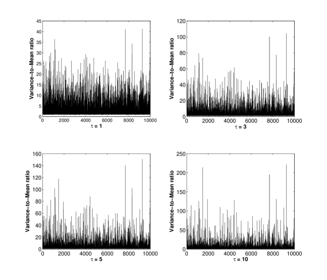
Figure 1: Variance-to-Mean ratios for a total of $10000$ simulated $\emph{MAP}_{2}$s for different values of $\tau$.

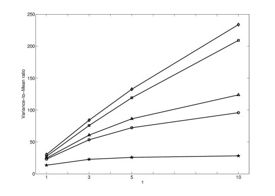
Figure 2: Variance-to-Mean ratios at time instants $\tau=1,3,5,10$, for $4$ randomly selected $\emph{MAP}_{2}$ representations.

3.2 Persistence measures

Next we shall study some persistence properties concerning the loss counting process of the $\emph{MAP}_{2}$. There are works in the literature which consider the modeling of persistence since this is an inherent phenomenon in many financial and insurance contexts, see for example Vallois and Tapiero, (2009); Stutzer, (2020) and the references therein. In general, in the OpRisk (and any financial) context it might be of interest to infer the probability that the next loss occurs in a short (or long) time given that the previous loss was recent (or far away). Also, decision makers could benefit from the knowledge of estimates for consecutive long periods without losses (long inter-loss times spells) or in contrast, short inter-loss times spells which might result in a higher capital charge. We next define these event and provide formulae for their calculation.

Let $s$ denote a fixed time. Recall from Section 2 that $T_{n}$ is the time elapsing from the occurrence of the $(n-1)$-th loss until the next ($n$-th) loss. Define the following persistence measures as

$$p_{01}(s) = P\left(T_{n+1}>s\mid T_{n}<s\right),$$

$$p_{11}(s) = P\left(T_{n+1}>s\mid T_{n}>s\right).$$

As previously commented, financial decision makers could be interested in estimating $1-p_{01}(s)$ for small values of $s$, or equivalently, the probability of the occurrence of a loss in a short period of time given that the previous loss occurred recently. Also, it would be advantageous to infer $p_{11}(s)$ for large values of $s$, that is, the probability of a long time up to the next loss given that the previous loss occurred long ago). In practice, $s$ can be chosen as a small or high percentile of a given historical trace of consecutive inter-loss times. Next result provides the expressions for the previous persistence measures.

Proposition 1.

Let a $\emph{MAP}_{2}$ be represented by $\{D_{0},D_{1}\}$. Let $P^{\star}$ denote the transition matrix between states where losses occur and $\phi$ its stationary distribution. Then,

$$p_{01}(s) = \frac{\mbox{\boldmath$\phi$}\left(I-e^{D_{0}s}\right)P^{\star}e^{D_{0}s}P^{\star}\mathbf{e}}{1-\mbox{\boldmath$\phi$}e^{D_{0}s}\mathbf{e}},$$ (17)

$$p_{11}(s) = \frac{\mbox{\boldmath$\phi$}e^{D_{0}s}P^{\star}e^{D_{0}s}P^{\star}\mathbf{e}}{\mbox{\boldmath$\phi$}e^{D_{0}s}\mathbf{e}},$$ (18)

for $s>0$.

See Appendix A for a proof.

Now, assume that the interest is to predict the probability of a sequence of short (long) inter-loss times spells. As before, consider a fixed time $s$. Then, define two discrete random variables $S$ and $L$ (standing for Short and Long, respectively) as

$$S=n \overset{d}{\equiv} \left(T_{1}<s\right)\cap\left(T_{2}<s\right)\cap\ldots\cap\left(T_{n}<s\right)\cap\left(T_{n+1}>s\right),$$ (19)

$$L=n \overset{d}{\equiv} \left(T_{1}>s\right)\cap\left(T_{2}>s\right)\cap\ldots\cap\left(T_{n}>s\right)\cap\left(T_{n+1}<s\right).$$ (20)

Defined as in (19)-(20), then for a small value of $s$, $S$ counts for the number of consecutive short inter-loss spells. On the other hand, if $s$ is large then, $L$ represents the number of consecutive long inter-loss spells. The following result expresses the probabilities of (19) and (20) in matrix form.

Proposition 2.

Let a $\emph{MAP}_{2}$ be represented by $\{D_{0},D_{1}\}$. Let $P^{\star}$ denote the transition matrix between states where losses occur and $\phi$ its stationary distribution. Then, for a fixed value $s>0$

$$P(S=n)=\left\{\begin{array}[]{lll}\mbox{\boldmath$\phi$}\left[\left(I-e^{D_{0}s}\right)P^{\star}\right]^{n}e^{D_{0}s}P^{\star}\mathbf{e},&\text{ if }&n\geq 1\\ &&\\ \mbox{\boldmath$\phi$}e^{D_{0}s}\mathbf{e},&\text{ if }&n=0.\end{array}\right.$$ (21)

$$P(L=n)=\left\{\begin{array}[]{lll}\mbox{\boldmath$\phi$}\left(e^{D_{0}s}P^{\star}\right)^{n}\left(I-e^{D_{0}s}\right)P^{\star}\mathbf{e},&\text{ if }&n\geq 1\\ &&\\ 1-\mbox{\boldmath$\phi$}e^{D_{0}s}\mathbf{e},&\text{ if }&n=0.\end{array}\right.$$ (22)

See Appendix B for a proof.

A remark is made at this point.

Remark 1.

Propositions 1 and 2 are also true for higher-order MAPs. This is because in the matrix expressions for the different persistence measures only $D_{0}$ is involved (and not $D_{1}$, or $D_{k}$ for $k\geq 2$ for higher-order MAPs). Also, the definitions of $P^{\star}$ and $\phi$ are common for MAPs of all orders, see Chakravarthy, (2001). In the case of higher-order MAPs the proofs shall be identical but changing the counter of the summation from $i,j,k\in\{1,2\}$ by $i,j,k\in\{1,2,\ldots,m\}$, being $m$ the order of the process.

To conclude this section, we present several numerical results in order to illustrate some of the patterns that (17)-(18) and (21)-(22) may follow. This issue is of paramount importance to determine the versatility of the $\emph{MAP}_{2}$ for modeling real-life situations. In this respect, the presented results are very preliminar and further research should be carried out in future work.

In order to illustrate some of the patterns that (17)-(18) and (21)-(22) are able to model, four different $\emph{MAP}_{2}$ representations were chosen:

1. $$D_{0}=\begin{pmatrix}-1.1272&\ 0.0055\\ 0&\ -42.4417\\ \end{pmatrix},\quad D_{1}=\begin{pmatrix}1.1217&\ 0\\ 0.2173&\ 42.2244\\ \end{pmatrix}.$$

2. $$D_{0}=\begin{pmatrix}-1.4373&\ 0.0498\\ 0&\ -14.2706\\ \end{pmatrix},\quad D_{1}=\begin{pmatrix}1.3875&\ 0\\ 0.5283&\ 13.7423\\ \end{pmatrix}.$$

3. $$D_{0}=\begin{pmatrix}-0.6830&\ 0.0026\\ 0&\ -34.6904\\ \end{pmatrix},\quad D_{1}=\begin{pmatrix}0&\ 0.6804\\ 34.5586&\ 0.1318\\ \end{pmatrix}.$$

4. $$D_{0}=\begin{pmatrix}-0.9751&\ 0.5933\\ 0&\ -46.6547\\ \end{pmatrix},\quad D_{1}=\begin{pmatrix}0&\ 0.3818\\ 10.7740&\ 35.8806\\ \end{pmatrix}.$$

The previous selection of parameters was made among a total of one million simulated $\emph{MAP}_{2}$s so that the four sets of parameters lead to different forms for expressions (17), (18), (21) and (22).

For each representation, $1-p_{01}(s)$ and $p_{11}(s)$ are computed for values of $s$ equal to the low percentiles ($5$-th,$6$-th,…,$49$-th and $50$-th) in the first case, and high percentiles ($50$-th,$51$-th,…,$94$-th and $95$-th) in the second case. The results are shown in Figures 3 and 4. Different models are obtained: in all the considered cases, the values of $1-p_{01}(s)$ increase with $s$ although the increase pattern differs between representations. On the contrary, there are cases where $p_{11}(s)$ is not monotonic.

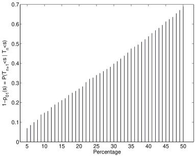
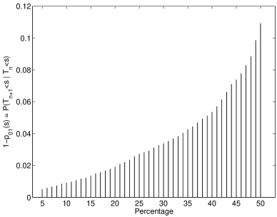
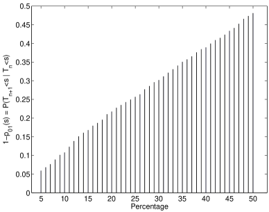
Figure 3: $P(T_{n+1}<s\mid T_{n}<s)$ for the four $\emph{MAP}_{2}$ representations: R1 (top left panel), R2 (top right panel), R3 (bottom left panel) and R4 (bottom right panel). The value of $s$ is determined by the percentiles of percentages given by the $X$-axis.

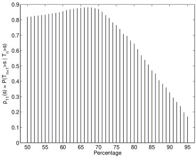
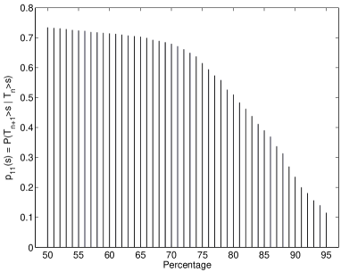
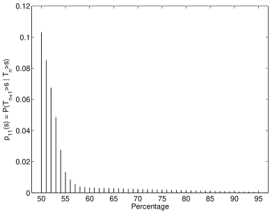
Figure 4: $P(T_{n+1}>s\mid T_{n}>s)$ for the four $\emph{MAP}_{2}$ representations: R1 (top left panel), R2 (top right panel), R3 (bottom left panel) and R4 (bottom right panel). The value of $s$ is determined by the percentiles of percentages given by the $X$-axis.

Figures 5 and 6 depict the probabilities of the random variables that count for the number of short and long inter-loss times. In particular, the value of $s$ has been chosen as the $20$-th and $80$-th percentiles of the inter-loss times distributions, respectively for $S$ and $L$. In the four cases, the probabilities mass functions are found to be unimodal at $0$ and rapidly decrease towards $0$, a pattern that was found in the total of the one million simulated $\emph{MAP}_{2}$s.

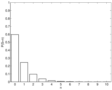
Figure 5: $P(S=n)$ for the four $\emph{MAP}_{2}$ representations: R1 (top left panel), R2 (top right panel), R3 (bottom left panel) and R4 (bottom right panel).

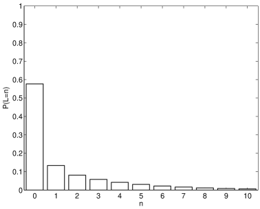
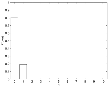
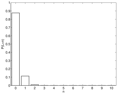
Figure 6: $P(L=n)$ for the four $\emph{MAP}_{2}$ representations: R1 (top left panel), R2 (top right panel), R3 (bottom left panel) and R4 (bottom right panel).

4 Modeling the OpRisk

According to the European Union Solvency II Directive for insurers (Groupe Consultatif Actuariel Européen,, 2007), the OpRisk is defined as “the risk of a change in value caused by the fact that actual losses, incurred for inadequate or failed internal processes, people and systems, or from external events, differ from the expected losses”. Because of its high expected impact to the banking industry, since the 9/11 attacks and tradings at Société Général, AIB and National Australia Bank, researchers have been studying approaches for properly modeling the OpRisk. The Basel II framework forces financial institutions to set aside a capital charge against unexpected losses derived from OpRisk. Three different methodologies have been proposed in the literature for OpRisk quantification: the Basic Indicator Approach, the Alternative Standardized Approach and, the most sophisticated one (in terms of statistical modeling), the Advanced Measurement Approach (AMA), where the Loss Distribution Approach (LDA) is included in. In the LDA the estimation of the annual loss distribution $Z$ as in (1) is achieved by modeling separately the distributions of the number of losses per year ($N$) and the severities ($X_{i}$), under the assumption of independence between them. It is common that the Poisson process or the Negative Binomial distribution are chosen to model the frequency, while some type of heavy-tailed distribution is selected to fit the severities, Chernobai et al., (2008); Bolancé et al., (2012). For a thorough treatment of the OpRisk modeling, we refer the reader to Panjer, 2006b ; Shevchenko, 2010b ; Bolancé et al., (2012); Peters and Shevchenko, (2015); Sharma, (2020).

The cumulative distribution function of $Z$ is calculated as

$$F_{Z}(x)=P\left(Z\leq x\right)=\sum_{n=0}^{\infty}P(N=n)F_{n}^{\star}(x),$$

where $F_{n}^{\star}(x)=P\left(X_{1}+\ldots,X_{n}\leq x\right)$ is the $n-$th convolution of the severities’ distribution. Although a closed-form expression for the loss aggregate distribution is usually hard to be obtained, its first and second moments can be computed in terms of those of the severity and frequency distributions as

$$E(Z) = E(N)E(X_{1}),$$

$$V(Z) = E(N)V(X_{1})+V(N)E(X_{1})^{2}.$$

Closed-form expressions for higher order moments can be found, for example in Shevchenko, 2010a . Under (1), the capital charge is obtained as the Value-at-Risk (VaR),

$$VaR_{p}\left(Z\right)=F_{Z}^{-1}(p),$$ (23)

where $F_{Z}^{-1}$ is the inverse cumulative distribution function of the total annual loss, and $p$ denotes the risk tolerance which is usually chosen close to 1. Another measure of interest in the OpRisk modeling is the expected shortfall (equivalently, conditional VaR), which unlike the VaR, satisfies the property of coherence. It is computed as

$$E\left(Z\mid Z\geq VaR_{p}(Z)\right).$$ (24)

If the distribution of $Z$ has an infinite mean, then clearly the expected shortfall does not exist.

In order to approximate (1) a battery of numerical methods, either based on simulations, inversion of characteristic functions, or recursions, have been proposed in the literature. For an exhaustive review of such methods, see Panjer, 2006b ; Shevchenko, 2010a ; Shevchenko, 2010b ; Gerhold et al., (2010), or Ch. 9 in Klugman et al., (2012).

5 Numerical application

In this section we illustrate an application of the $\emph{MAP}_{2}$ in the context of the OpRisk. In particular, given a real OpRisk database, described in Section 5.1, the $\emph{MAP}_{2}$ is fitted to the times between consecutive losses in Section 5.2. Descriptors of interest associated to the distributions of the inter-loss times and the number of yearly losses, as well as estimations for the persistence measures described in Section 3 are obtained. In Section 5.3 the severities’ distribution are modeled through the heavy-tailed, double Pareto Lognormal distribution. As will be seen, the combination of the $\emph{MAP}_{2}$ for the frequency with the heavy-tailed model for the loss severity distribution, will enable us to give an estimate of the loss aggregate model and the capital charge in Section 5.4.

5.1 Data description

The real OpRisk data set considered in this paper consists of $225$ records of loss occurrences and associated severities in a Spanish financial institution. The sample, which corresponds to a unique risk cell (retail banking Basel II business line), was obtained from $4929$ consecutive days ($13.5$ years) in the period between 30/12/1993 and 29/06/2007. In a total of $225$ out of the $4929$ days, a single loss occurred which was recorded together with the corresponding severity. Some descriptors of the dataset are as follows. The average, median, variation coefficient and maximum value of the inter-loss times are $22.0045$, $8$, $2.827$ and $667$ days. Also, the empirical correlation coefficient is non-negligible and given by $0.3546$. For the severities, the average, median, variation coefficient and maximum are $151710$, $34318$, $2.0973$ and $2289060$. Note that, from the empirical values both samples are right-skewed with a tail longer than that of an exponential distribution. This can also deduced from Figure 7, which depicts the empirical quantiles in comparison to those of the fitted (via MLE) exponential distributions. Note how the larger empirical quantiles are far from the fitted ones.

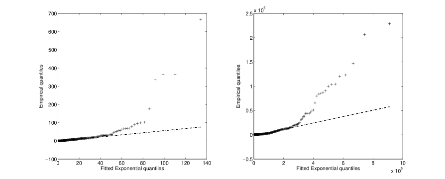
Figure 7: QQ-plots of the empirical inter-loss times (left panel) and severities (right panel) quantiles versus those of the fitted exponential distributions.

5.2 The estimated frequency distribution

In this section we describe how the database inter-loss times are modeled by the $\emph{MAP}_{2}$. The estimated (joint) distribution of the times, the modeling of the counting process $N(\tau)$ and of the persistence measures described in Section 3 will be analyzed.

The distribution of the inter-loss times

The methodology from Section 2.3 was applied to fit a $\emph{MAP}_{2}$ to the sample of inter-loss times, and the obtained results were as follows. First, the estimated process was found as

$$\widehat{D}_{0}=\left(\begin{array}[]{cc}-0.0063&0.0011\\ 0&-0.1036\end{array}\right),\qquad\widehat{D}_{1}=\left(\begin{array}[]{cc}0.0052&0\\ 0.0016&0.1020\end{array}\right).$$ (25)

Very closed values were obtained if instead the Bayesian algorithm by Ramírez-Cobo et al., (2017) is considered.

The mean, median, coefficient of variation and correlation coefficient under the estimated model were $22.0047$, $7.52$, $2.8205$ and $0.3545$, all close to the empirical values commented in Section 5.1. The estimated $\emph{MAP}_{2}$ (25) defines a theorical cdf as in (8) which is plotted in dashed line in Figure 8 together with the empirical cdf of the data (solid line). The performance of the exponential distribution is also shown in dotted line. The outperformance of the PH-distribution (which defines the inter-loss times distribution in a $\emph{MAP}_{2}$) over the classic exponential distribution is clear from this figure.

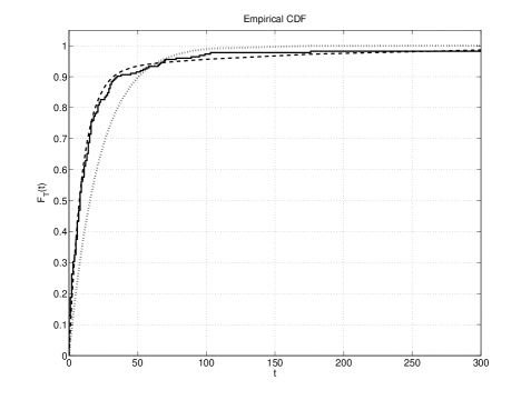
Figure 8: Inter-loss times cdf: empirical (solid line) versus estimated by the $\emph{MAP}_{2}$ (dashed line) and, by the exponential distribution (dotted line).

The distribution of the number of losses per year

We turn out to the estimation of the counting process. As commented in Section 5.1 losses were recorded in a period of length between $13$ and $14$ years. It was found that the average number of losses per year is equal to $16.6154$, and the variance is $342.9231$. In this respect, the Poisson process presents again a poor performance, since it would notably underestimate the sample variance. Given the estimated $\emph{MAP}_{2}$ (25), the expected number of losses as well as the variance were computed according to (14)-(15), and found as $16.5874$ and $240.0192$.

Since the modeling of the frequency in the OpRisk context usually refers to the one year horizon, the numerical algorithm described in Rodríguez et al., (2015) was applied to obtain the estimates of the probabilities as in (13), for $\tau=365$. Hence, from now on, $N$ will denote $N(365)$. Figure 9 depicts the obtained mass function of $N$, the annual number of losses, which will be used in Section 5.4 for approximating the loss aggregate distribution. Note that the obtained probabilities cannot be compared against their empirical versions because of the small sample size (a sample of $13$ years). We finally would like to point out the differences between the adjusted mass function and that of a Poisson distribution. The first is unimodal around $0$, but it is non-negligible for high losses; in contrast, the Poisson mass function of rate $16.6154$ (equal to the average number of annual losses) concentrates around its mean with a much smaller variance.

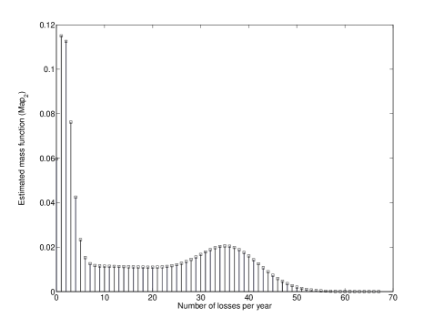
Figure 9: Number of losses per year. Estimated mass function under the $\emph{MAP}_{2}$.

Persistence measures

Here we obtain the estimates of (17)-(18) and (21)-(22) for the real inter-loss times, according to the MLE estimates (25).

Consider first the estimation of the conditional probability of a next short (long) inter-loss time assuming that the previous inter-loss time was short (long). It is importante to remark that due to the small sample sizes, the empirical values of the transition probabilities $1-p_{01}(s)$ were not calculated for values of $s$ less than the $30$-th percentile of the inter-loss times distribution. In analogous way, $p_{11}(s)$ was not estimated from the sample for values of $s$ larger than the times distribution’s $70$-th percentile. As a result, the empirical values of $1-p_{01}(s)$ were estimated for $s$ equal to the $30$-th, $35$-th,…,$50$-th percentiles. These percentiles define for each case the length of the short inter-loss time. Similarly, the empirical probabilities $p_{11}(s)$ were estimated for $s$ ranging between the $50-$th, $55$-th,…,$70$-th percentiles (defining the long times). The empirical values (represented with a triangle) and the estimated values (represented by a circle) are depicted by Figure 10. In the figure, the white bars refer to the $1-p_{01}(s)$ values while the black bars concern the probabilities $p_{11}(s)$. Consider for example, the $30$-th percentile of the dataset (found as $s=3$). Then, the empirical value of $P(T_{n+1}<3\mid T_{n}<3)$ was $0.3731$ (that is, the $37.31\%$ of inter-loss times satisfying $T<3$ were followed by times that also satisfied the condition). This value is represented by the first white bar ending in a triangle. In this case, the fit given by the $\emph{MAP}_{2}$ (equal to $0.262$ and represented by the next white bar ending in a circle), clearly underestimated the empirical value. However, there are examples where the $\emph{MAP}_{2}$ provides good estimates. For instance, if $s$ is chosen as the $60$-th percentile (found as $s=11$), then the empirical probability $P(T_{n+1}>11\mid T_{n}>11)$ was $0.4787$, and the $\emph{MAP}_{2}$ provided an estimated value equal to $0.4340$.

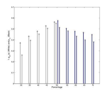
Figure 10: White bars: $P(T_{n+1}<s\mid T_{n}<s)$, for $s=30,35,40,45,50$-th percentiles. Blues bars: $P(T_{n+1}>s\mid T_{n}>s)$, for $s=50,55,60,65,70$-th percentiles. Triangles denote empirical values and circles denote estimated values.

Consider next the estimation of the probabilities of short and long spells, as in (21)-(22). As in the previous case, $s=3$ is considered for the study of $S$ (sequence of short spells), and $s=11$ for that of $L$ (sequence of long spells). Figure 11 depicts the estimated probabilities for values of $n=0,1,\ldots,10$. For both examples, the functions are unimodal at $0$ but with non-negligible values for the cases $n=1,2$. The empirical values for the probabilities $P(S=0)$, $P(S=1)$ and $P(S=2)$ were $0.7366$, $0.0804$ and $0.0670$. The estimated values, shown by the first three bars in the left panel of the figure, where $0.7535$, $0.1419$ and $0.0476$, respectively. If the interest is in the sequence of long spells, the empirical values for the probabilities $P(L=0)$, $P(L=1)$ and $P(L=2)$ were $0.6161$, $0.1875$ and $0.0580$ and the estimated ones were $0.6291$, $0.2101$ and $0.0759$.

Figure 11: Estimated values for the mass probability functions of the short ($S$, left panel) and long ($L$, right panel) spells of the OpRisk dataset.

5.3 The estimated severities’ distribution

Concerning the severity distribution, we fit the data by a double Pareto Lognormal (dPlN) distribution. Such distribution has been suggested in the literature as a versatile heavy-tailed model able to correctly model both the tail and body of the distribution and also, to capture different forms of asymmetry. See for example, Reed and Jorgensen, (2004) or Ramírez-Cobo et al., (2010). We briefly recall its definition. A random variable $X$ follows a double Pareto Lognormal distribution with parameters $\left(\alpha,\beta,\mu,\sigma^{2}\right)$ if $X=e^{Y}$ where $Y$ is random variable distributed according a Normal Laplace distribution, that is, $Y=Z+W$, where $Z\sim N\left(\mu,\sigma^{2}\right)$, and $W$ is distributed according a skewed Laplace model, that is,

$$f_{W}(w|\alpha,\beta)=\left\{\begin{array}[]{cl}\frac{\alpha\beta}{\alpha+\beta}e^{\beta w}&\mbox{if $w\leq 0$,}\\ \frac{\alpha\beta}{\alpha+\beta}e^{-\alpha w}&\mbox{if $w>0$,}\end{array}\right.$$

independent of $Z$, for $\alpha,\beta>0$.

Reed and Jorgensen, (2004) illustrate the form of the dPlN density function for various different groups of parameter values. In particular, they show that it exhibits heavy-tail behavior, since $f_{X}(x)\rightarrow kx^{-\alpha-1}$ as $x\rightarrow\infty$. The dPlN distribution lacks a closed form expression for its moment generating function. Nevertheless, if $r<\alpha$, the moment of order $r$ is given by

$$E\left(X^{r}\mid\alpha,\beta,\mu,\sigma^{2}\right)=\frac{\alpha\beta}{(\alpha-r)(\beta+r)}e^{r\mu+r^{2}\sigma^{2}/2}.$$

The approach for Bayesian estimation of the dPlN distribution in Ramírez-Cobo et al., (2010) was applied to fit the severity data sample. The (posterior) expected values for the parameters of the model were $\left(\alpha,\beta,\mu,\sigma^{2}\right)=(1.24,\ 1.8,\ 10.4,\ 1.29^{2})$. Note that, since $\alpha<2$ then, the estimated distribution has a finite mean but an infinite variance. The fit to the histogram of the severities sample (in log-scale) by the dPlN distribution is shown by Figure 12, as well as the fits by other heavy-tailed models typically used in the OpRisk contexts, namely, the Lognormal, Weibull, Pareto and Generalized Pareto. It can be seen how the first three have a poorer performance that the dPlN, while the Generalized Pareto was comparable.

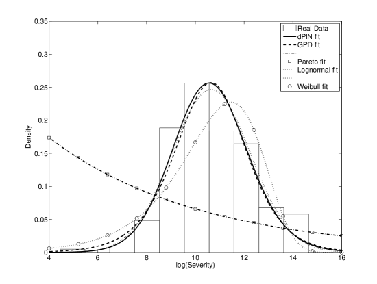
Figure 12: Histogram and fitted pdf for the real severities in log-scale under the dPlN model (solid line) and benchmark approaches.

5.4 The estimated loss aggregate distribution and risk measures

From the estimates obtained in Sections 5.2 and 5.3 we make inference here for the loss aggregate model (1). As commented in Section 4, a number of numerical strategies do exist in order to estimate (1). Comparing the different approaches is out of the scope in this paper, and here for simplicity, we shall approximate the loss aggregate distribution by the classic, Monte Carlo (MC) method. The steps to implement the MC algorithm are shown in Table 1.

1. For $k=1,\ldots,K$, (a) Simulate the number of annual losses, $N$, from the estimated $\emph{MAP}_{2}$ given by (25). The estimated mass function of $N$ to be used is depicted by Figure 9. (b) Given that $N=n$, simulate independent severities $X_{1},\ldots,X_{n}$ from the dPlN distribution estimated in Section 5.3, with parameters $\left(\alpha,\beta,\mu,\sigma^{2}\right)=(1.24,\ 1.8,\ 10.4,\ 1.29^{2})$. (c) Compute $Z_{k}=\sum_{i=1}^{n}X_{i}$. 2. Set $k=k+1$ and return to 1.

Table 1: Monte Carlo algorithm to sample from the loss aggregate distribution.

Once the samples $(Z_{1},\ldots,Z_{k})$ from the loss aggregate distribution are obtained, the risk measures (23) and (24) can be easily estimated by their empirical counterparts.

One of the main drawbacks of the MC algorithm is its typical slow convergence, specially in presence of heavy tails, see for example Brunner et al., (2009); Shevchenko, 2010a . In order to choose an appropriate number of simulations $K$, the following numerical exercise was considered. A total of $K$ samples of $Z$, for $K\in\{10^{4},10^{5},10^{6},10^{7}\}$, were obtained $500$ times, from which the corresponding estimated $VaR_{99.9\%}$s were recorded. The $500$ samples of the $VaR_{99.9\%}$ under the four considered values of $K$ are depicted in Figure 13. It can be noted that under $K=10^{7}$, the convergence is achieved.

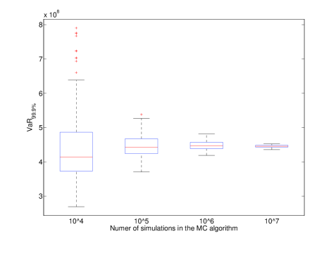
Figure 13: Boxplot of the samples of $VaR_{99.9\%}$ ($500$ values each), for different values of $K$.

Section 5.2 showed the outperformance of the $\emph{MAP}_{2}$ with respect to the Poisson process when fitting the loss occurrence process. It is natural to wonder if such encountered differences affect the estimated compound models and related risk measures. To address this issue, the algorithm in Table 1 was implemented, also for $K=10^{7}$, but here the distribution of the annual losses $N$ in point 1.(a) was set to a Poisson distribution of rate equal to the average number of annual losses ($16.6154$). The obtained results evidence the sensitivity of the aggregate loss distribution to the choice of the occurrence process. Table 2 summarizes both aggregate distributions by means of an assortment of descriptive statistics (minimum and maximum values, mean, standard deviation, skewness and different quantiles). The values have been divided by $10^{7}$ for abbreviation reasons. A first remark to be made is that the minimum value and the 0.025 quantile of $Z$ under the $\emph{MAP}_{2}$ are equal to zero. Indeed, there exists a proportion (around $6\%$) of null samples of $Z$. This is a consequence of the non-negligible probability that $N=0$, under the $\emph{MAP}_{2}$ (see Figure 9). This phenomenon is rarely observed under the considered Poisson process for which $P(N=0)\approx 6\times 10^{-8}$ is obtained. Second, as expected (see Embrechts et al., (1997)), both distributions are positive skewed with a long right tail as a consequence of the heavy-tailed severities. In all cases (with the exception of the 0.025 quantile), the quantiles and mean of $Z$ are larger under the $\emph{MAP}_{2}$ than under the Poisson process. This can be explained again by the mass function of the annual occurrences under the two considered point processes: while for the Poisson process $P(N\geq 30)=0.002$, this probability changes to $0.2836$, under the $\emph{MAP}_{2}$. This implies that for some years, a very high number of losses may occur under the $\emph{MAP}_{2}$, and this makes the loss aggregate distribution take more extreme values than under the Poisson process.

	$\min$	$\max$	mean	SD	$\gamma$	$Q_{.025}$	$Q_{.25}$	$Q_{.50}$	$Q_{.975}$
$\emph{MAP}_{2}$	0	$8420$	$1.4$	$16$	321.9	0	0.72	0.99	4.47
Poisson	$0.00045$	$5000$	$0.41$	$8.6$	431.6	0.0525	0.1303	0.2073	1.44

Table 2: Values (divided by $10^{7}$) for the descriptive statistics of the aggregate loss distribution $Z$ under the $\emph{MAP}_{2}$ and Poisson process.

Finally, Table 3 shows the risk measures of interest for the financial entities: the $VaR_{p}$ and $ES_{p}$ (see Eq. 23-24), for $p\in\{0.99,0.999\}$ and under the two point processes. The shown values are divided by $10^{8}$ and $10^{9}$, respectively. Here again, the results suggest that under the $\emph{MAP}_{2}$ process, higher potential losses than under the Poisson process may occur, and in consequence, the capital charge increases in significant way.

	$VaR_{p}$		$ES_{p}$
	$p=0.99$	$p=0.999$	$p=0.99$	$p=0.999$
$\emph{MAP}_{2}$	0.8068	4.405	0.3181	1.6887
Poisson	0.27	1.575	0.1209	0.613

Table 3: $VaR_{p}$ and $ES_{p}$ values (divided by $10^{8}$ and $10^{9}$, respectively) under the $\emph{MAP}_{2}$ and Poisson process, for $p\in\{0.95,0.99,0.999\}$.

6 Conclusions

In this paper, an aggregate loss model with occurrence process governed by a type of Markov renewal process has been considered. The selected stochastic process is the $\emph{MAP}_{2}$ which allows for correlated and non-exponential inter-loss times and also for overdisperse loss counts. We have shown in Section 3 how the $\emph{MAP}_{2}$ mostly produces loss counts presenting a variance significantly higher than the mean, a feature that highlights its applicability in financial contexts. One of the novelties of the paper is the derivation of some persistence measures that may help the financial decision makers when evaluating the historical trace of loss times. The aggregate loss model has been estimated by modeling in separate way the frequency from the severity distributions. For the first, an approach based on the direct maximization of the likelihood function of the inter-loss times distributions, has been explored. The application of the methodology to the OpRisk modeling constitutes a significant contribution of the work. A real OpRisk data set representing inter-loss times and associated severities is fitted: for comparison reasons, the times are modeled by both the $\emph{MAP}_{2}$ and the Poisson process, and for the severities the same heavy-tailed distribution is considered. The outperformance of the $\emph{MAP}_{2}$ in fitting the occurrence process leads to important differences in the estimated loss aggregate distribution and related risk measures, which points out the sensitivity of the aggregate loss distribution to the choice of the frequency distribution in this case.

The authors aim to test the potential for modeling aggregate loss distributions of the Batch Markovian arrival process (BMAP), an extension of the MAP which allows for simultaneous (and correlated) losses, see Lucantoni, (1991, 1993). Several perspectives may be considered in this respect. First, and similarly as in the present paper, the BMAP can be thought as a model for the frequency while any type of heavy-tailed distribution is chosen for the severity. In principle, this approach would show more versatility and applicability than the MAP because in real risk scenarios different losses may occur at the same time. Second, the previous approach could be extended to model aggregate loss distributions more than one cell via the superposition of differently parametrized BMAPs. From the statistical inference viewpoint the BMAP represents a partially solved problem, mainly because of its non-identifiability, lack of a known canonical representation and consequent numerical troubles. Finally, as already commented throughout the manuscript, a more detailed inspection of the formulae for the persistence measures should be undertaken. In particular, given the aspect of the mass probability functions for the sequence of spells, it is of interest to study the possible connection with zero-inflated models. Work on these issues is underway.

Appendix A: Derivation of the expressions for $p_{01}(s)$ and $p_{11}(s)$

The proof is a consequence of the theory of Markov renewal processes. All results used in this Appendix can be found in Ch. 10 in Çinlar, (1975).

First, $p_{01}(s)$ is written as

$$p_{01}(s)=\frac{P(T_{n+1}>s,T_{n}<s)}{P(T_{n}<s)},$$ (26)

where according to (8), $P(T_{n}<s)=F_{T}(s)=1-\mbox{\boldmath$\phi$}e^{D_{0}s}\mathbf{e}$. Recall that since the $\emph{MAP}_{2}$ is a Markov renewal process, then the sequences of states $\{Y_{n}\}_{n=1}^{\infty}$ at the times of the losses is a Markov chain with transition matrix $P^{\star}$. Consider the semi-Markov kernel $Q(\cdot)$ as in (3) over the state space $\mathcal{S}=\{1,2\}$. Then, by definition of semi-Markov kernel, for $i,j\in\mathcal{S}$, $t>0$,

$$Q_{i,j}(t)=P(Y_{n+1}=j,T_{n+1}\leq t\mid Y_{n}=i),$$

which represents the $(i,j)$-th element of the semi-Markov kernel $Q(t)$. Also, define

$$G(i,j,t)=\frac{Q_{i,j}(t)}{P^{\star}(i,j)},\ i,j\in\mathcal{S},t>0,$$

where $G(i,j,t)=1$ in case $P^{\star}(i,j)=Q_{i,j}(t)=0$. Then, $G(i,j,\cdot)$ is a cumulative distribution function

$$G(i,j,t)=P(T_{n+1}\leq t\mid Y_{n}=i,Y_{n+1}=j).$$

Finally, the following paramount property is key for our proof. This states that given the Markov chain, then the inter-loss times are conditionally independent, or in other words,

$$P(T_{1}\leq u_{1},\ldots,T_{n}\leq u_{n}\mid Y_{0},\ldots,Y_{n})=G(Y_{0},Y_{1},u_{1})G(Y_{1},Y_{2},u_{2})\ldots G(Y_{n-1},Y_{n},u_{n}).$$

Consider the numerator in (26). This can be rewritten as

$$P(T_{n}<s,T_{n+1}>s)=$$ (27)

$$\sum_{i,j,k\in\{1,2\}}\bigl{\{}P(T_{n}<s,T_{n+1}>s\mid Y_{n-1}=i,Y_{n}=j,Y_{n+1}=k)\times\bigr{.}$$

$$\hskip 48.36958pt\bigl{.}\times P(Y_{n-1}=i,Y_{n}=j,Y_{n+1}=k)\bigr{\}}=$$

$$\sum_{i,j,k\in\{1,2\}}\bigl{\{}P(T_{n}<s,T_{n+1}>s\mid Y_{n-1}=i,Y_{n}=j,Y_{n+1}=k)\times\bigr{.}$$

$$\hskip 48.36958pt\bigl{.}\times P(Y_{n+1}=k\mid Y_{n}=j,Y_{n-1}=i)P(Y_{n}=j,Y_{n-1}=i)\bigr{\}}=$$

$$\sum_{i,j,k\in\{1,2\}}\bigl{\{}P(T_{n}<s,T_{n+1}>s\mid Y_{n-1}=i,Y_{n}=j,Y_{n+1}=k)\times\bigr{.}$$

$$\hskip 48.36958pt\bigl{.}\times P(Y_{n+1}=k\mid Y_{n}=j)P(Y_{n}=j\mid Y_{n-1}=i)P(Y_{n-1}=i)\bigr{\}}=$$

$$\sum_{i,j,k\in\{1,2\}}\bigl{\{}P(T_{n}<s,T_{n+1}>s\mid Y_{n-1}=i,Y_{n}=j,Y_{n+1}=k)\times\bigr{.}$$

$$\hskip 48.36958pt\bigl{.}\times P^{\star}(i,j)\ P^{\star}(j,k)\ \phi_{i}\bigr{\}}=$$

$$\sum_{i,j,k\in\{1,2\}}G\left(i,j,s\right)\left(1-G(j,k,s)\right)P^{\star}(i,j)\ P^{\star}(j,k)\ \phi_{i}=$$

$$\sum_{i,j,k\in\{1,2\}}\frac{Q_{i,j}(s)}{P^{\star}(i,j)}\left(1-\frac{Q_{j,k}(s)}{P^{\star}(j,k)}\right)P^{\star}(i,j)\ P^{\star}(j,k)\ \phi_{i}=$$

$$\sum_{i,j,k\in\{1,2\}}\frac{Q_{i,j}(s)}{P^{\star}(i,j)}\left(\frac{P^{\star}(j,k)-Q_{j,k}(s)}{P^{\star}(j,k)}\right)P^{\star}(i,j)\ P^{\star}(j,k)\ \phi_{i}=$$

$$\sum_{i,j,k\in\{1,2\}}Q_{i,j}(s)\bigl{(}P^{\star}(j,k)-Q_{j,k}(s)\bigr{)}\phi_{i}.$$ (28)

It is a straightforward computation to check that (Appendix A: Derivation of the expressions for $p_{01}(s)$ and $p_{11}(s)$) can be expressed in matrix form as

$$\sum_{i,j,k\in\{1,2\}}Q\left(i,j,s\right)\bigl{(}P^{\star}(j,k)-Q(j,k,s)\bigr{)}\phi_{i}=\mbox{\boldmath$\phi$}Q(s)\bigl{(}P^{\star}-Q(s)\bigr{)}\mathbf{e}.$$ (29)

From (3) and (4) one obtains

$$\mbox{\boldmath$\phi$}Q(s)\bigl{(}P^{\star}-Q(s)\bigr{)}\mathbf{e}=\mbox{\boldmath$\phi$}\left(I-e^{D_{0}s}\right)P^{\star}e^{D_{0}s}P^{\star}\mathbf{e},$$

which concludes the proof for the expression of $p_{01}$. Finally, the proof for the matrix formulation of $p_{11}$ is obtained in analogous way.

Appendix B: Derivation of the expressions for $P(S=n)$ and $P(L=n)$

Consider first the case $n=0$. Then, from (8)

$$P(S=0)=P(T_{n+1}>s)=1-F_{T}(s)=\mbox{\boldmath$\phi$}e^{D_{0}s}\mathbf{e},$$

and similarly for the variable $L$. If instead $n\geq 1$, the proof follows closely the derivation of (27). Indeed, by a recursive argument,

$$P(S=n) = P(T_{1}<s,T_{2}<s,\ldots,T_{n}<s,T_{n+1}>s)=$$

$$\sum_{i_{1},i_{2},\ldots,i_{n+2}\in\{1,2\}}\bigl{\{}P\left(T_{1}<s,T_{2}<s,\ldots,T_{n}<s,T_{n+1}>s\mid Y_{0}=i_{1},Y_{1}=i_{2},\ldots,Y_{n}=i_{n+1},Y_{n+1}=i_{n+2}\right)\times\bigr{.}$$

$$\bigl{.}\times P(Y_{0}=i_{1},Y_{1}=i_{2},\ldots,Y_{n}=i_{n+1},Y_{n+1}=i_{n+2})\bigr{\}}=$$

$$\ldots=$$

$$\sum_{i_{1},i_{2},\ldots,i_{n+2}\in\{1,2\}}G\left(i_{1},i_{2},s\right)G\left(i_{2},i_{3},s\right)\cdots G\left(i_{n},i_{n+1},s\right)\bigl{(}1-G(i_{n+1},i_{n+2},s)\bigr{)}P^{\star}(i_{1},i_{2})\cdots P^{\star}(i_{n+1},i_{n+2})\phi_{i_{1}}=$$

$$\sum_{i_{1},i_{2},\ldots,i_{n+2}\in\{1,2\}}\bigl{(}\prod_{l=1}^{n}G\left(i_{l},i_{l+1},s\right)\bigr{)}\bigl{(}1-G(i_{n+1},i_{n+2},s)\bigr{)}\bigl{(}\prod_{l=1}^{n}P^{\star}\left(i_{l},i_{l+1}\right)\bigr{)}\ P^{\star}(i_{n+1},i_{n+2})\ \phi_{i_{1}}=$$

$$\sum_{i_{1},i_{2},\ldots,i_{n+2}\in\{1,2\}}\bigl{(}\prod_{l=1}^{n}Q_{i_{l},i_{l+1}}(s)\bigr{)}\ \bigl{(}P^{\star}(i_{n+1},i_{n+2})-Q_{i_{n+1},i_{n+2}}(s)\bigr{)}\phi_{i_{1}}.$$

Then,

$$\sum_{i_{1},i_{2},\ldots,i_{n+2}\in\{1,2\}}\bigl{(}\prod_{l=1}^{n}Q_{i_{l},i_{l+1}}(s)\bigr{)}\ \bigl{(}P^{\star}(i_{n+1},i_{n+2})-Q_{i_{n+1},i_{n+2}}(s)\bigr{)}\phi_{i_{1}}=\mbox{\boldmath$\phi$}Q^{n}(s)\bigl{(}P^{\star}-Q(s)\bigr{)}\mathbf{e},$$

and from (3) and (4),

$$\mbox{\boldmath$\phi$}Q^{n}(s)\bigl{(}P^{\star}-Q(s)\bigr{)}\mathbf{e}=\mbox{\boldmath$\phi$}\left[\left(I-e^{D_{0}s}\right)P^{\star}\right]^{n}e^{D_{0}s}P^{\star}\mathbf{e}.$$

To see that (21) is indeed a mass probability function, we next show that $\sum_{n=0}^{\infty}P(S=n)=1$. First, from Ch. 4 in Janssen and Manca, (2006), one has

$$\lim_{n\rightarrow\infty}Q^{n}(s)=\mathbf{0},$$

which implies that $\sum_{n=1}^{\infty}Q^{n}(s)=Q(s)(I-Q(s))^{-1}$. Then,

$$\sum_{n=0}^{\infty}P(S=n) = \mbox{\boldmath$\phi$}e^{D_{0}s}\mathbf{e}+\sum_{n=1}^{\infty}\mbox{\boldmath$\phi$}Q^{n}(s)e^{D_{0}s}P^{\star}\mathbf{e}$$

$$= \mbox{\boldmath$\phi$}e^{D_{0}s}\mathbf{e}+\mbox{\boldmath$\phi$}Q(s)(I-Q(s))^{-1}e^{D_{0}s}P^{\star}\mathbf{e}$$

$$= \mbox{\boldmath$\phi$}e^{D_{0}s}\mathbf{e}+\mbox{\boldmath$\phi$}Q(s)(I-Q(s))^{-1}(P^{\star}-Q(s))\mathbf{e}$$

$$= \mbox{\boldmath$\phi$}e^{D_{0}s}\mathbf{e}+\mbox{\boldmath$\phi$}Q(s)(I-Q(s))^{-1}(P^{\star}\mathbf{e}-Q(s)\mathbf{e})$$

$$= \mbox{\boldmath$\phi$}e^{D_{0}s}\mathbf{e}+\mbox{\boldmath$\phi$}Q(s)(I-Q(s))^{-1}(\mathbf{e}-Q(s)\mathbf{e})$$

$$= \mbox{\boldmath$\phi$}e^{D_{0}s}\mathbf{e}+\mbox{\boldmath$\phi$}Q(s)(I-Q(s))^{-1}(I-Q(s))\mathbf{e}$$

$$= \mbox{\boldmath$\phi$}e^{D_{0}s}\mathbf{e}+\mbox{\boldmath$\phi$}Q(s)\mathbf{e}$$

$$= \mbox{\boldmath$\phi$}\left(e^{D_{0}s}+P^{\star}-e^{D_{0}s}P^{\star}\right)\mathbf{e}$$

$$= \mbox{\boldmath$\phi$}e^{D_{0}s}\mathbf{e}+\mbox{\boldmath$\phi$}P^{\star}\mathbf{e}-\mbox{\boldmath$\phi$}e^{D_{0}s}P^{\star}\mathbf{e}$$

$$= \mbox{\boldmath$\phi$}e^{D_{0}s}\mathbf{e}+1-\mbox{\boldmath$\phi$}e^{D_{0}s}\mathbf{e}$$

$$= 1$$

In the previous set of formulae we applied that since $P^{\star}$ is a stochastic matrix, then $P^{\star}\mathbf{e}=\mathbf{e}$. Also, since $\phi$ represents its stationary probability vector, then $\mbox{\boldmath$\phi$}P^{\star}=\mbox{\boldmath$\phi$}$.

Finally, the proof for $P(L=n)$ is immediate following a similar reasoning.

References

- Ahn and Badescu, (2007) Ahn, S. and Badescu, A. L. (2007). On the analysis of the Gerber–Shiu discounted penalty function for risk processes with Markovian arrivals. Insurance: Mathematics and Economics, 41(2):234–249.
- Ausín et al., (2011) Ausín, M., Vilar, J., Cao, R., and González-Fragueiro, C. (2011). Bayesian analysis of aggregate loss models. Mathematical Finance, 21(2):257–279.
- Avanzi et al., (2016) Avanzi, B., Wong, B., and Yang, X. (2016). A micro-level claim count model with overdispersion and reporting delays. Insurance: Mathematics and Economics, 71:1 – 14.
- Badescu et al., (2007) Badescu, A., Drekic, S., and Landriault, D. (2007). On the analysis of a multi-threshold Markovian risk model. Scandinavian Actuarial Journal, 2007(4):248–260.
- Bodrog et al., (2008) Bodrog, L., Heindlb, A., Horváth, G., and Telek, M. (2008). A Markovian canonical form of second-order matrix-exponential processes. European Journal of Operational Research, 190:459–477.
- Bolancé et al., (2012) Bolancé, C., Guillén, M., Gustafsson, J., and Nielsen, J. P. (2012). Quantitative Operational Risk Models. Chapmal & Hall, CRC Press.
- Brechmann et al., (2014) Brechmann, E., Czado, C., and Paterlini, S. (2014). Flexible dependence modeling of operational risk losses and its impact on total capital requirements. Journal of Banking & Finance, 40:271–285.
- Breuer, (2002) Breuer, L. (2002). An EM algorithm for batch Markovian arrival processes and its comparison to a simpler estimation procedure. Annals of Operations Research, 112:123–138.
- Brunner et al., (2009) Brunner, M., Piacenza, F., Monti, F., and Bazzarello, D. (2009). Fat tails, expected shortfall and the Monte Carlo method: a note. The Journal of Operational Risk, 4(1):81–88.
- Carrizosa and Ramírez-Cobo, (2014) Carrizosa, E. and Ramírez-Cobo, P. (2014). Maximum likelihood estimation in the two-state Markovian arrival process.
- Casale et al., (2010) Casale, G., Z. Zhang, E., and Simirni, E. (2010). Trace data characterization and fitting for Markov modeling. Performance Evaluation, 67:61–79.
- Çinlar, (1975) Çinlar, E. (1975). Introduction to stochastic processes. Prentice-Hall, Usa.
- Chakravarthy, (2001) Chakravarthy, S. (2001). The Batch Markovian arrival process: a review and future work. In et al., A. K., editor, Advances in probability and stochastic processes, pages 21–49.
- Chakravarthy, (2009) Chakravarthy, S. (2009). A disaster queue with Markovian arrivals and impatient customers. Applied Mathematics and Computation, 214:48–59.
- Chapelle et al., (2004) Chapelle, A., Crama, Y., Hubner, G., and Peters, J. (2004). Basel II and operational risk: Implications for risk measurement and management in the financial sector. National Bank of Belgium Working Paper, No. 51.
- Chavez-Demoulin et al., (2015) Chavez-Demoulin, V., Embrechts, P., and Hofert, M. (2015). An extreme value approach for modeling operational risk losses depending on covariates. Journal of Risk and Insurance.
- Chavez-Demoulin et al., (2006) Chavez-Demoulin, V., Embrechts, P., and Nešlehová, J. (2006). Quantitative models for operational risk: extremes, dependence and aggregation. Journal of Banking & Finance, 30(10):2635–2658.
- Chernobai et al., (2008) Chernobai, A. S., Rachev, S. T., and Fabozzi, F. J. (2008). Operational risk: a guide to Basel II capital requirements, models, and analysis, volume 180. John Wiley & Sons.
- Cheung and Landriault, (2010) Cheung, E. and Landriault, D. (2010). A generalized penalty function with the maximum surplus prior to ruin in a MAP risk model. Insurance: Mathematics and Economics, 46:127–134.
- Cheung et al., (2018) Cheung, E., Liu, H., and Willmot, G. (2018). Joint moments of the total discounted gains and losses in the renewal risk model with two-sided jumps. Applied Mathematics and Computation, 331:358–377.
- Cheung et al., (2009) Cheung, E. C., Landriault, D., et al. (2009). Perturbed MAP risk models with dividend barrier strategies. Journal of Applied Probability, 46(2):521–541.
- Cope and Antonini, (2008) Cope, E. and Antonini, G. (2008). Observed correlations and dependencies among operational losses in the ORX consortium database. Journal of Operational Risk, 3(4):47–74.
- Cruz, (2002) Cruz, M. (2002). Modeling, Measuring and Hedging Operational Risk. John Wiley & Sons.
- Dimitrova et al., (2016) Dimitrova, D., Kaishev, V., and Zhao, S. (2016). On the evaluation of finite-time ruin probabilities in a dependent risk model. Applied Mathematics and Computation, 275:268–286.
- Dutta and Perry, (2007) Dutta, K. and Perry, J. (2007). A tale of tails: an empirical analysis of loss distribution models for estimating operational risk capital. Working paper 06-13, Federal Reserve Bank of Boston.
- Embrechts et al., (2003) Embrechts, P., Höing, A., and Juri, A. (2003). Using copulae to bound the Value-at-Risk for functions of dependent risks. Finance and Stochastics, 7:145–167.
- Embrechts et al., (1997) Embrechts, P., Klüppelberg, C., and Mikosch, T. (1997). Modelling extremal events: for insurance and finance, volume 33. Springer Science & Business Media.
- Eum et al., (2007) Eum, S., Harris, R., and Atov, I. (2007). A matching model for MAP-2 using moments of the counting process. In Proceedings of the International Network Optimization Conference, INOC 2007, Spa, Belgium.
- Fearnhead and Sherlock, (2006) Fearnhead, P. and Sherlock, C. (2006). An exact Gibbs sampler for the Markov-modulated Poisson process. Journal of the Royal Statistical Society: Series B (Statistical Methodology), 68(5):767–784.
- Feria-Domínguez et al., (2015) Feria-Domínguez, J., Jiménez-Rodríguez, E., and Sholarin, O. (2015). Tackling the over-dispersion of operational risk: implications on capital adequacy requirements. The North American Journal of Economics and Finance, 31:206–221.
- Fodra and Pham, (2015) Fodra, P. and Pham, H. (2015). High frequency trading and asymptotics for small risk aversion in a markov renewal model. SIAM Journal on Financial Mathematics, 6(1):656–684.
- Frostig, (2008) Frostig, E. (2008). On ruin probability for a risk process perturbed by a Lévy process with no negative jumps. Stochastic Models, 24(2):288–313.
- Fung et al., (2019) Fung, T., Badescu, A., and Lin, X. (2019). Multivariate Cox hidden Markov models with an application to operational risk. Scandinavian Actuarial Journal, 2019(8):686–710.
- Gerhold et al., (2010) Gerhold, S., Schmock, U., and Warnung, R. (2010). A generalization of Panger’s recursion and numerically stable risk aggregation. Finance and Stochastics, 14:81–128.
- Groupe Consultatif Actuariel Européen, (2007) Groupe Consultatif Actuariel Européen (2007). Solvency II Glossary: European Commission. Technical report.
- Heffes and Lucantoni, (1986) Heffes, H. and Lucantoni, D. (1986). A Markov modulated characterization of packetized voice and data traffic and related statistical multiplexer performance. IEEE Journal on Selected Areas in Communications, 4:856–868.
- Janssen and Manca, (2006) Janssen, J. and Manca, R. (2006). Applied Semi-Markov Processes. Springer.
- Kim et al., (2017) Kim, C., Klimenok, V., and Dudin, A. (2017). Analysis of unreliable BMAP/PH/N type queue with Markovian flow of breakdowns. Applied Mathematics and Computation, 314:154–172.
- Klemm et al., (2003) Klemm, A., Lindemann, C., and Lohmann, M. (2003). Modeling IP traffic using Batch Markovian Arrival Process. Performance Evaluation, 54(2):149–173.
- Klugman et al., (2012) Klugman, S. A., Panjer, H. H., and Willmot, G. E. (2012). Loss models: from data to decisions. John Wiley & Sons.
- Lindsey, (1995) Lindsey, J. (1995). Modelling frequency and count data, volume 15. Oxford University Press.
- Lucantoni, (1991) Lucantoni, D. (1991). New results for the single server queue with a Batch Markovian Arrival Process. Stochastic Models, 7:1–46.
- Lucantoni, (1993) Lucantoni, D. (1993). The queue: A tutorial. In Donatiello, L. and Nelson, R., editors, Models and Techniques for Performance Evaluation of Computer and Communication Systems, pages 330–358. Springer, New York.
- Lucantoni et al., (1990) Lucantoni, D., Meier-Hellstern, K., and Neuts, M. (1990). A single-server queue with server vacations and a class of nonrenewal arrival processes. Advances in Applied Probability, 22:676–705.
- Maegebier, (2013) Maegebier, A. (2013). Valuation and risk assessment of disability insurance using a discrete time trivariate Markov renewal reward process. Insurance: Mathematics and Economics, 53(3):802–811.
- McNeil et al., (2015) McNeil, A. J., Frey, R., and Embrechts, P. (2015). Quantitative Risk Management: Concepts, Techniques and Tools. Princeton university press.
- Mittnik and Yener, (2009) Mittnik, S. and Yener, T. (2009). Estimating operational risk capital for correlated, rare events. Journal of Operational Risk, 4(4):1–23.
- Narayana and Neuts, (1992) Narayana, S. and Neuts, M. F. (1992). The first two moment matrices of the counts for the Markovian arrival process. Communications in statistics. Stochastic models, 8(3):459–477.
- Nasr et al., (2018) Nasr, W., Charanek, A., and Maddah, B. (2018). MAP fitting by count and inter-arrival moment matching. Stochastic Models (in Press).
- Neuts and Li., (1997) Neuts, M. and Li., J. (1997). An algorithm for the matrices of a continuous BMAP, volume 183 of Lectures notes in Pure and Applied Mathematics, pages 7–19. Srinivas R. Chakravarthy and Attahiru, S. Alfa, editors. NY: Marcel Dekker, Inc.
- Neuts, (1979) Neuts, M. F. (1979). A versatile Markovian point process. Journal of Applied Probability, 16:764–779.
- Ng and Yang, (2006) Ng, A. C. and Yang, H. (2006). On the joint distribution of surplus before and after ruin under a Markovian regime switching model. Stochastic Processes and their Applications, 116(2):244–266.
- Nystrom and Skoglund, (2002) Nystrom, K. and Skoglund, J. (2002). Quantitative operational risk management. Working paper, Swedbank, Group Financial Risk Control.
- Okamura and Dohi, (2016) Okamura, H. and Dohi, T. (2016). Fitting phase-type distributions and Markovian arrival processes: Algorithms and tools. In Principles of performance and reliability modeling and evaluation, pages 49–75.
- (55) Panjer, H. H. (2006a). Aggregate Loss Modeling. John Wiley & Sons, Ltd.
- (56) Panjer, H. H. (2006b). Operational risk: modeling analytics. John Wiley & Sons.
- Peters and Shevchenko, (2015) Peters, G. W. and Shevchenko, P. V. (2015). Advances in Heavy Tailed Risk Modeling: A Handbook of Operational Risk. John Wiley & Sons.
- Pfeifer and Nešlehová, (2004) Pfeifer, D. and Nešlehová, J. (2004). Modeling and generating dependent risk processes for IRM and DFA. Astin Bulletin, 34(02):333–360.
- Ramírez-Cobo et al., (2010) Ramírez-Cobo, P., Lillo, R., and Wiper, M. (2010). Nonidentifiability of the two-state Markovian arrival process. Journal of Applied Probability, 47(3):630–649.
- Ramírez-Cobo et al., (2017) Ramírez-Cobo, P., Lillo, R., and Wiper, M. (2017). Bayesian analysis of the stationary MAP2. Bayesian Analysis, 12(4):1163–1194.
- Ramírez-Cobo et al., (2010) Ramírez-Cobo, P., Lillo, R. E., Wilson, S., and Wiper, M. P. (2010). Bayesian inference for Double Pareto lognormal queues. Annals of Applied Statistics, 4(3):1533–1557.
- Ramírez-Cobo et al., (2014) Ramírez-Cobo, P., Marzo, X., Olivares-Nadal, A. V., Francoso, J.-A., Carrizosa, E., and Pita, M. F. (2014). The Markovian arrival process: A statistical model for daily precipitation amounts. Journal of Hydrology, 510(0):459 – 471.